Light Euclidean Spanners with Steiner Points
Abstract
The FOCS’19 paper of Le and Solomon [62], culminating a long line of research on Euclidean spanners, proves that the lightness (normalized weight) of the greedy -spanner in is for any and any (where hides polylogarithmic factors of ), and also shows the existence of point sets in for which any -spanner must have lightness .111The lightness of a spanner is the ratio of its weight and the MST weight. Given this tight bound on the lightness, a natural arising question is whether a better lightness bound can be achieved using Steiner points.
Our first result is a construction of Steiner spanners in with lightness , where is the spread of the point set.222The spread of a point set in is the ratio of the largest to the smallest pairwise distance. In the regime of , this provides an improvement over the lightness bound of [62]; this regime of parameters is of practical interest, as point sets arising in real-life applications (e.g., for various random distributions) have polynomially bounded spread, while in spanner applications often controls the precision, and it sometimes needs to be much smaller than . Moreover, for spread polynomially bounded in , this upper bound provides a quadratic improvement over the non-Steiner bound of [62], We then demonstrate that such a light spanner can be constructed in time for polynomially bounded spread, where hides a factor of . Finally, we extend the construction to higher dimensions, proving a lightness upper bound of for any and any .
1 Introduction
A -spanner for a set of points in the -dimensional Euclidean space is a geometric graph that preserves all the pairwise Euclidean distances between points in to within a factor of , called the stretch factor; by geometric graph we mean a weighted graph in which the vertices correspond to points in and the edge weights are the Euclidean distances between the corresponding points. The study of Euclidean spanners dates back to the seminal work of Chew [29, 30] from 1986, which presented a spanner with constant stretch and edges for any set of points in . In the three following decades, Euclidean spanners have evolved into an important subarea of Discrete and Computational Geometry, having found applications in many different areas, such as approximation algorithms [68], geometric distance oracles [45, 48, 47, 46], and network design [55, 63]; see the book by Narasimhan and Smid “Geometric Spanner Networks” [64] for an excellent account on Euclidean spanners and some of their applications. Numerous constructions of Euclidean spanners in two and higher dimensions were introduced over the years, such as Yao graphs [73], -graphs [31, 57, 58, 69], the (path-)greedy spanner [4, 25, 64] and the gap-greedy spanner [70, 6]— unveiling an abundance of techniques, tools and insights along the way; refer to the book of [64] for more spanner constructions.
In addition to low stretch, many applications require that the spanner would be sparse, in the unweighted and/or weighted sense. The sparsity (respectively, lightness) of a spanner is the ratio of its size (respectively, weight) to the size (resp., weight) of a spanning tree (resp., MST), providing a normalized notion of size (resp., weight), which should ideally be . For any dimension , spanners with constant sparsity are known since the 80s [73, 31, 57, 58, 69, 4, 70, 6]; also, it is known since the early 90s that the greedy spanner has constant lightness [4]. The constant bounds on the sparsity and lightness depend on both and . In some applications, must be a very small sub-constant parameter, so as to achieve the highest possible precision and minimize potential errors, and in some situations may be as small as for some constant . Consequently, besides the theoretical appeal, achieving the precise dependencies on and in the sparsity and lightness bounds is of practical importance.
Culminating a long line of work, in FOCS’19 Le and Solomon [62] showed that the precise dependencies on in the sparsity and lightness bounds are and , respectively, for any and any ; throughout we shall use to hide polylogarithmic factors of . The lower bounds of [62] are proved for the -dimensional sphere, for . On the upper bound side, sparsity is achieved by a number of classic constructions such as Yao graphs [73], -graphs [31, 57, 58, 69], the (path-)greedy spanner [4, 25, 64] and the gap-greedy spanner [70, 6], and the argument underlying all these upper bounds is basic and simple. On the other hand, constant lightness upper bound (regardless of the dependency on and ) is achieved only by the greedy algorithm [4, 33, 34, 68, 64, 44, 14, 62], and all known arguments for constant lightness are highly nontrivial, even for ; in fact, the proofs in [4, 33, 34, 68] have missing details. The first complete proof was given in the book of [64], in a 60-page chapter, where it is shown that the greedy -spanner has lightness , which improved the dependencies on and given in all previous work. In SODA’19, Borradaile, Le and Wulff-Nilsen [14] presented a shorter and arguably simpler alternative proof that applies to the wider family of doubling metrics, which improves the dependency provided in FOCS’15 by Gottlieb [44] for doubling metrics, but is inferior to the lightness bound of by [64].333The doubling dimension of a metric space is the smallest value such that every ball in the metric space can be covered by at most balls of half the radius of . This notion generalizes the Euclidean dimension, since the doubling dimension of the Euclidean space is . A metric space is called doubling if its doubling dimension is constant. Finally, the lightness bound of of [62] was proved via a tour-de-force argument; interestingly, the proof for is much more intricate than for higher dimensions .
Le and Solomon [62] showed that, counter-intuitively, one can use Steiner points to bypass the sparsity lower bound of Euclidean spanners. Specifically, in this way they reduced the sparsity upper bound almost quadratically to , and also provided a matching lower bound for . Their lower bound for sparsity is derived from a lightness lower bound; specifically, they first prove that, for a set of points evenly spaced on the boundary of the unit square, with distances between neighboring points, any Steiner -spanner must incur lightness , and then they translated the lightness lower bound into a sparsity lower bound of . Whether or not Steiner points can be used to reduce the lightness remained open in [62], but this should not come as a surprise.444The lightness of Steiner spanners can be defined with respect to the SMT (Steiner minimum tree) weight, but we can also stick to the original definition, since the SMT and MST weights differ by a constant factor smaller than 2. First, bounding the lightness of spanners is inherently more difficult than bounding their sparsity— this is true for both Euclidean spaces and doubling metrics, as well as other graph families including general weighted graphs [4, 33, 34, 68, 64, 44, 14, 62, 28, 42, 36]. Second, constructing Steiner trees and spanners with asymptotically improved bounds is inherently more difficult than constructing their non-Steiner counterparts [37, 38, 71, 60, 12, 61]. In our particular case, while the classic sparsity upper bound for non-Steiner Euclidean spanners is simple, its improved counterpart for Steiner spanners by [62] requires a number of nontrivial insights and is rather intricate. On the other hand, the lightness upper bound of [62] uses a tour-de-force argument, and as mentioned already this is true even for . Consequently, obtaining an improved lightness bound using Steiner points seems currently out of reach, at least until an inherently simpler proof to [62] for non-Steiner lightness is found (if one exists).
1.1 Our Contribution.
In this paper, we explore the power of Steiner points in reducing lightness for Euclidean spaces of bounded spread .555The spread of a Euclidean space is the ratio of the maximum to minimum pairwise distances in it. Point sets of bounded spread have been studied extensively for Euclidean spanners and related geometric objects [9, 56, 32, 54, 18, 17, 39, 67, 1, 2, 5, 52, 53, 20, 65, 66, 19, 72, 23]. The motivation for studying point sets of bounded spread is three-fold.
-
1.
Such point sets arise naturally in practice, and are thus important in their own right; indeed, for many random distributions, the spread is polynomial in the number of points— in expectation and with high probability. In particular, it is known that for -point sets drawn uniformly at random from the unit square, the expected spread is , and the expected spread in the unit -dimensional hypercube is for any . Researchers have studied random distributions of point sets, in part to explain the success of solving various geometric optimization problems in practice [9, 56, 32], and there are many results on spanners for random point sets [26, 7, 40, 10, 41, 15, 64, 72, 16, 23, 8, 59]. Of course, the family of bounded spread point sets is much wider than that of random point sets.
-
2.
Euclidean spanners can be constructed in (deterministic) time in such point sets [21], while there is no -time algorithm for constructing Euclidean spanners in arbitrary point sets. (The result of [21] extends to other geometric objects, such as WSPD and compressed quadtrees, and some of the aforementioned references (e.g., [53, 18]) build on this result to achieve faster algorithms for other geometric problems for point sets of polynomially bounded spread.)
- 3.
As mentioned above, Le and Solomon [62] showed that for a set of points evenly spaced on the boundary of the unit square, with distances between neighboring points, any Steiner -spanner must incur lightness . Note that the spread of this point set is . The non-Steiner upper bound for by [62] is . A natural arising question is whether one can improve the lightness upper bound of using Steiner points, ideally quaratically, for point sets of bounded spread. We answer this question in the affirmative.
Theorem 1.1.
Any point set in of spread admits a Steiner -spanner of lightness .
Recalling that the lower bound of by [62] applies to a point set of spread , the lightness upper bound provided by Theorem 1.1 is therefore tight (up to polylogarithmic factors in ) for point sets of spread . Moreover, this upper bound improves the general upper bound of from [62] in the regime , i.e., when . For spread polynomial in , we get an improvement over [62] as long as . Of course, the improvement gets more significant as decays— in the most extreme situation is inverse polynomial in , and then the improvement over [62] is polynomial in even when is exponential in .
Our second result is that a Steiner spanner with near-optimal lightness can be constructed in linear time, when the spread is polynomial in .
Theorem 1.2.
For any point set in of spread , for any , a Steiner -spanner of lightness can be constructed in time, where hides a factor of .
Higher dimensions
The lower bound of [61] states that any (non-Steiner) -spanner must incur lightness , for any . We show that, similarly to the 2-dimensional case, one can improve the lightness almost quadratically using Steiner points, for point sets of bounded spread.
Theorem 1.3.
For any , any point set in of spread admits a Steiner -spanner of lightness .
Interestingly, the dependence on the spread in the lightness bound provided by Theorem 1.3 does not grow with the dimension, hence the improvement over the non-Steiner bound gets more significant as the dimension grows, provided of course that the spread is not too large.
Follow-up Work
Recently Bhore and Tóth [11] proved a lightness lower bound for Steiner spanners of a point set with spread for any . Their lower bound for improved the lower bound in Le and Solomon [62] by a factor of . This implies that our upper bound in Theorem 1.3 is almost tight (up to a factor of ) for point set with spread . On the positive side, using directional -spanners, they showed that point set in admits a Steiner -spanner with lightness . This bound improved the lightness bound in Theorem 1.1 when the spread is super-polynomial in .
1.2 Proof Overview
1.2.1 Proof of Theorem 1.1
We partition the set of pairs of points into subsets where contains pairs of distances in . The objective is to show that one can preserve distances between all pairs in to within a factor of using a Steiner spanner of weight ; by taking the union of all such spanners, we obtain a Steiner spanner with the required lightness.
Let . A natural idea to preserve distances in is to (a) find an -net 666A subset of points is an -net if every point in is within distance from (or covered by) some point in and pairwise distances between points in are larger than . of and (b) add to the spanner edges between any two net points and such that and there is a pair in such that and are covered by (i.e., within distance from) and , respectively. The stretch will be in check because and are at distance roughly from their net points and thus, the additive stretch between and is . For lightness, we can show that the number of net points , and using a (nontrivial) packing argument, there are about edges of length added in step (b). Thus, the total weight of the spanner is , which is bigger than our aimed lightness bound by a factor of .
To shave the factor of , we employ two ideas. First, we take to be a -net of . In this way . By applying the 2-dimensional Steiner spanner construction of [62] as a blackbox, we obtain a Steiner spanner with only edges of length that approximates distances between points in ; we have thus reduced the weight bound to , as required. The problem now is with the stretch guarantee: Preserving distances between the points in is no longer sufficient. Indeed, for every pair , the distance between and to the nearest net points is , hence the resulting stretch is . We overcome this hurdle by introducing a novel construction of single-source spanners, which generalize Steiner shallow-light trees of Solomon [71]. Specifically, we open the black-box of [62] and observe that every time we want to preserve the distance from (some) Steiner point to a net-point , instead of connecting to by a straight line of weight , we can use a single-source spanner (rooted at ) of weight to preserve distances (up to a factor) from to every point within distances from . As a result, our Steiner spanner can preserve distances between any two points to within a factor of , where , , and are their nearest net points.
Replacing by
A factor incurred in the lightness bound of Theorem 1.1 is because we have subsets . To reduce to , we observe that and that we can take every edge of weight at most to the spanner since all such edges have total weight at most . Thus, the pairs of interest now have weights in the range and hence we set .
1.2.2 Proof of Theorem 1.3
By extending the construction in Theorem 1.1, we can construct a Steiner spanner with lightness as follows: for each , we construct an -net and then apply the construction of [62] as a black box to obtain a Steiner spanner for with weight . The stretch will be in check since is an -net. Since , . The union of Steiner spanners for all has weight . Note when , we can not take as a -net since the construction of single-source spanners with weight in the proof of Theorem 1.1 only works when .
Most of our effort is to further refine the result in a way that term is multiplied only by and not by the term that depends on . We first reduce to the problem of approximating distances between pairs (of endpoints) in a family of edge sets with , where edges of have length (roughly) in the interval and edges in have length in . Let . For a technical reason, we will subdivide edges of by using a set of Steiner points so that each new edge has length in .
We construct a Steiner spanner for edges in using a charging cover tree : has depth , level of is associated with an -cover777A subset of points is an -cover if every point in is within distance from some point in . of , and leaves (at level ) of are points in . For each cover at level of , we construct a graph where and there is an edge between if there is a corresponding edge in whose endpoints are covered by and , respectively. Graph is used to distinguish between low degree points, whose degree in is , and high degree points, whose degree in is . will have two charging properties: (1) every point has at least uncharged descendants and (2) at every level , one can charge up to uncharged descendants of high degree points. Note that, once an uncharged point is charged at level , it will be marked as charged at higher levels; initially at level , every point is uncharged.
We then use a charging cover tree to guide the Steiner spanner construction. Specifically, at level , we add all edges incident to low degree points to the spanner and we can show that the total weight of all these edges over all levels is at most . For high degree points, we apply the construction of Le and Solomon [62] to obtain a Steiner spanner , and we charge the weight of to uncharged descendants of each high degree point. This charging is possible by the charging property (2) of . We then show that each point in is charged a weight at most . Thus, the total weight of the Steiner spanners (for high degree points) at all levels is .
Our construction of a charging cover tree is inspired by the construction of a hierarchy of clusters in the iterative clustering technique. The technique was initially developed by Chechick and Wulff-Nilsen [27] to construct light spanners for general graphs, and then was adapted to many other different settings [27, 13, 14, 62, 61]. Our construction is directly inspired by the construction of Borradaile et al. [14] in the doubling dimension setting. However, our construction is much simpler. Specifically, we are able to decouple the Steiner spanner construction from the charging cover tree construction. We refer readers to Section 5 for more details.
Replacing by
Using the same technique pointed in the previous section, by taking every edge of weight at most to the spanner, we are left with pairs of weights in range . Thus, we can set instead of .
2 Preliminaries
Let be a point set of points in . We denote by the Euclidean distance between two points . Let be the ball of radius centered at . Given a point and a set of point on the plane, we define the distance between and , denoted by , to be .
An -cover of is a subset of points such that for every point , there is at least one point such that ; we say is covered by . When the value of is clear from the context, we simply call a cover of . A subset of point is called an -net if is an -cover of and also an -packing of , i.e., for every two points , .
Let be a graph with weight function on the edges. We denote the vertex set and edge set of by and , respectively. Let be the distance between two vertices of . We denote by the subgraph induced by a subset of vertices .
is geometric in if each vertex of corresponds to a point and for every edge , . In this case, we use points to refer to vertices of . We say that a geometric graph is a -spanner of if and for every two points , . We say that is a Steiner -spanner for if and for every two points , . Points in are called Steiner points. Note that distances between Steiner points may not be preserved in a Steiner -spanner.
3 Steiner Spanners on the Plane
We focus on constructing a Steiner spanner with good lightness; the fast construction is in Section 4. We will use the following geometric Steiner shallow-light tree (SLT) construction by Solomon [71].
Lemma 3.1.
Let be a line segment of length and be a point on the plane such that . For any point set , there is a geometric graph of weight such that for any point .
We will use single-source spanners (defined below) as a black box in our construction.
Definition 3.2 (Single-source spanners).
Given a point (source), a set of points on the plane and a connected geometric graph spanning , a single source -spanner w.r.t. is a graph such that for every : .
Our starting point is the construction of a single source spanner from a point to point set enclosed in a circle of radius such that . We show that, if approximately preserves the distances between pairs of points in up to a factor for any constant , it is possible to construct a single-source spanner with weight . It is not so hard to see that if Steiner points are not allowed, a lower bound of weight holds here.
Lemma 3.3.
Let be a set of points in a circle of radius on the plane and a point of distance from . Let be a -spanner of for any constant . Then there is a single-source -spanner w.r.t. of weight when .
Proof: Let be a center of . W.l.o.g, we assume that is parallel to -axis. Let be the axis-aligned smallest square bounding . Observe that the side length of is at mos . Place a grid on , so that every cell of is a square of side length . Observe that:
We extend to by connecting an (arbitrary) corner of each grid cell to an arbitrary point of in the cell. Observe that: . Let be the set of grid points on the side, say , of that is closer to (than the opposite side). We apply the construction in Lemma 3.1 to and to obtain a geometric graph . Let . Since by Lemma 3.1, it holds that .
It remains to show the stretch bound. Let be any point of and be the point in the same cell with that is connected to a corner, say of grid . We will show below that:
| (1) |
If Equation 1 holds, it would imply:
Thus, it remains to prove Equation 1. To this end, let be the projection of on . (Point is also a grid point; see Figure 1) Let be projections of and on the line containing , respectively. Let be the intersection of and . Observe that . Thus,
| (2) |
Since and by Lemma 3.1, we have:
| (3) |
which implies Equation 1.
r

We obtain the following corollary of Lemma 3.3.
Corollary 3.4.
Let be a set of points in a circle of radius on the plane and a point of distance from for some constant . Let be a -spanner of for any constant . Then there is a single-source -spanner w.r.t. of weight when .
Proof: We scale the space by . In the scaled space, has radius and . Let , where , be circles of radius covering ; such a set of circles can be constructed greedily. We apply Lemma 3.3 to and each to construct a single-source -spanner from to each . The final spanner is that has total weight in the scaled metric. Thus, in the original metric, . We are now ready to prove Theorem 1.1.
Proof: [Proof of Theorem 1.1] Assume that the minimum pairwise distance is . Let be all pairs of points. Partition into sets where is the set of pairs such that .
For a fixed , we claim that there is a geometric graph such that for every two distinct points , and that . Thus, is a Steiner spanner with weight .
We now focus on constructing . Let . We will construct a spanner with stretch for some constant . By induction, we can assume that:
| (4) |
for any pair .
Let and be a -net of . For each point , let be the net point that covers : the distance from to is at most .
Claim 3.5.
.
Proof: Consider the circle centered at ; contains a segment of length of the MST, which is not contained in any other circle. Thus, the claim holds.
Next, we consider the smallest axis-aligned square bounding the point set. In the following, we divide into a set of (overlapping) sub-squares of side length each. This way, for any pair (of distance at most ), there is a sub-square entirely containing , and the balls of radius around the two net points.
Constructing We first divide into subsquares of side length each888We assume that the side length of is divisible by ; otherwise, we can extend in such a way.. For each subsquare , we extend its borders equally to four directions by an amount of in each direction. After this extension, has side length .
Claim 3.6.
Every point in belongs to at most subsquares in . Furthermore, for each pair , there is a subsquare such that are entirely contained in .
Proof: Let be a subsquare in containing one of the endpoints of , say , before extension. Then, after extension, will contain both since , and furthermore, and are at least away from the boundary since we extended by in each direction. Thus, points in () will be at most from () when .
Consider a subsquare . Let . By abusing notation, we denote by all the pairs in of . We will show that:
Claim 3.7.
There is a Steiner spanner of weight at most such that for any pair of points , it holds that:
for some big enough constant .
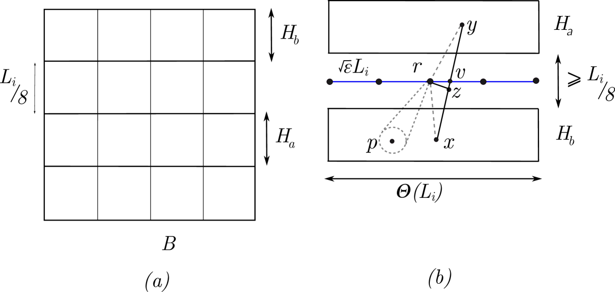
Proof: We divide into horizontal (vertical) bands of length (width) so that for any two points , and are in two non-adjacent horizontal bands and/or vertical bands (see Figure 2). These bands exist since
Now for each pair of non-adjacent horizontal bands and , . Draw a bisecting segment (touching two sides of ) between and and place equally-spaced Steiner points, say , on the bisecting line in a way that the distance between any two nearby Steiner points is (see Figure 2(a)). For each point , and each net point , we apply the construction of Corollary 3.4 to , the set of endpoints of inclosed in circle and ; let be the obtained geometric graph (see Figure 2(b)). Note that . Thus, by Corollary 3.4, and that:
| (5) |
for any . Let . It holds that
Let . Then, we have:
| (6) |
We apply the same construction for every pair of non-adjacent vertical bands. We then let be the union of all for every pair of non-adjacent horizontal/vertical bands . It holds that:
| (7) |
since there are only pairs of bands. To bound the stretch, let be a pair in whose endpoints are in . W.l.o.g, assume that are two non-adjacent horizontal bands that contain and , respectively. Let be the intersection of segment and the bisecting line of (see Figure 2(b)). Let be the closest Steiner point to in and be the projection of on . Observe that when . We have:
4 A Linear Time Construction
In this section, we assume that for some constant , and is a constant. We use the same model of computation used by Chan [21]: the real-RAM model with word size and floor function. We will use notation to hide a polynomial factor of . Chan [21] showed that:
Theorem 4.1 (Step 4 in [21]).
Given a poin set with spread for constant and , a -spanner of can be constructed in time.
We will use a construction of an -net for a point set for any in time . Such a construction was implicit in the work of Har-Peled [51] which was made explicit by Har-Peled and Raichel (Lemma 2.3 [53]).
Lemma 4.2 (Lemma 2.3 and Corollary 2.4 [53]).
Given and an -point set in , an -net of can be constructed in time. Furthermore, for each net point , one can compute all the points covered by in total time.
We first show that the spanner in Corollary 3.4 can be implemented in time.
Claim 4.3.
The single-source spanner in Corollary 3.4 can be found in time.
Proof: First, we observe that the single source spanner in Lemma 3.3 can be constructed in time . This is because the grid has size and the SLT tree from to (a set of grid points on) can be constructed in time. The single-source spanner in Corollary 3.4 uses a constant number of constructions construction in Lemma 3.3. Thus, the total running time is .
Proof: [Proof of Theorem 1.2]
Our implementation will follow the construction in Section 3 ; we will reuse notation in that section as well. Let be a -spanner for constructed in time by Theorem 4.1. In our fast construction algorithm, instead of considering all pairs of points , we only consider the pairs corresponding to edges of ; there are such pairs. Our algorithm has four steps:
-
•
Step 1 Partition pairs of endpoints in into at most sets where is the set of pairs such that . Let . This step can be implemented in time . The following steps are applied to each . Let be the set of endpoints of . We observe that:
(9) -
•
Step 2 Construct a -net for in time using the algorithm in Lemma 4.2.
-
•
Step 3 Compute a bounding square and divide it into (overlapping) subsquares of length each. Let be the set of subsquares that contain at least one point participating in the pairs . Since there are only non-empty subsquares, can be computed in time by iterating over each point and check (in time) which subsquare the point falls into. Here we use the fact that each floor operation takes time.
-
•
Step 4 For each subsquare , we divide it into horizontal bands and vertical bands of length . For each pair of non-adjacent (horizontal) bands , construct a set of Steiner points on the bisecting line between and as in Section 3. For each Steiner point and each net point , we apply Corollary 3.4 to construct a single source spanner from to a set of points ; this step can be implemented in time by Claim 4.3. By Claim 3.6, the construction in this step can be implemented in time. Our final spanner is the union of all single source spanners in all subsquares in .
The running time needed to implement Steps 2 to 4 is by Equation 9. The same analysis in Section 3 gives lightness. For stretch, we observe that the stretch of the spanner for each edge of is . Thus, the stretch for every pair of points in is . We can recover stretch by setting where is the constant behind big-O.
5 Steiner Spanners in High Dimension
In this section, we a light Steiner spanner for a point set with spread as in Theorem 1.3. We rescale the metric so that every edge in has weight at least . Let be the minimum spanning tree of . We subdivide each edge of length , by placing Steiner points greedily, in a way that each new edge has length at least and at most . Let be the set of Steiner points. We observe that:
| (10) |
Let be some parameter and . Let be the set of edges such that
| (11) |
where . If an edge for some , we will abuse notation by saying that . The main focus of this section is to show that:
Lemma 5.1.
There is a Steiner spanner that preserves distances between the endpoints of edges in with weight .
Proof: [Proof of Theorem 1.3] We assume that is a power of . We partition the interval into intervals . For each fixed , let , and be the set of edges with in the definition of . Recall that we scale the metric so that every edge in has weight at least . Thus,
Observe that for all . By Lemma 5.1, there exists a Steiner spanner with weight preseving distances between endpoints of edges in up to a factor. Then is a Steiner -spanner with weight .
We now focus on constructing a Steiner spanner in Lemma 5.1. We will use the following Steiner spanner construction as a black box.
Theorem 5.2 (Theorem 1.3 [62]).
For a given point set , there is a Steiner -spanner, denoted by , with edges that preserves pairwise distances of points in up to a factor.
We will rely on a cover tree to construct a Steiner spanner. Let be a sufficiently big constant chosen later ().
Definition 5.3 (Cover tree).
A cover for point set with levels has each node associated with a point of such that (a) level- of is the point set , (b) level- of is associated with a -cover of and (c) .
A point may appear in many levels of a cover tree . To avoid confusion, we denote by the copy of at level , and we still call a point of . For each point , we denote by and the set of children and descendants of in , respectively. Note that includes .
We will construct the Steiner spanner level by level, starting from level . At every level, we will add a certain set of edges to . We then charge the weight of a subset of the edges to a subset of uncharged points of ; initially, every point of is uncharged. To decide which uncharged points we will charge to at level , we consider a geometric graph where and there is an edge between two points (of weight ) in if there exists at least one between two descendants of and , respectively. We say a cover point has high degree if its degree in is at least . At level , we only charge to uncharged points which are descendants of high degree cover points. The intuition is that high cover points have many descendants. This leads to a notion of a charging cover tree. We call a cover tree a charging cover tree for if for all level ,
-
(1)
Each point has at least descendants that are uncharged at level less than .
-
(2)
Up to uncharged descendant of each high-degree cover point can be charged at level . No descendant of low-degree points is charged at level .
We show how to construct a charging cover tree in Appendix 5.4. We now show that given a charging cover tree, we can construct a Steiner spanner with the lightness bound in Lemma 5.1. Let be such a charging cover tree. We define a set of edges as follows:
| (12) |
We abuse notation by denoting the graph induced by the set of edges in .
Claim 5.4.
and for any and every , .
Proof: Edges in can be partitioned according to levels where an edge is at level if it connects a point and its parent. Observe that at level , the total edge weight is at most times the number of points and hence, the total weight is by Equation 10. At higher level, we observe that the total weight of edges of at level is at most , and that since each point has by property (1) of the charging tree. Thus, the total weight of edges at level at least is at most:
This implies the weight bound of . We now bound the distance between . Let be the (unique) path from to . By construction, for . This implies:
when . Similarly, and hence . Claim 5.4 implies that the descendants of any level node in a charging cover tree form a subgraph of diameter at most . Let be the set of edges that will be our final spanner. Initially, . We will abuse notation by denoting the graph induced by edge set .
5.1 Spanner construction at level
Recall that is a geometric graph where and there is an edge between two points in if there exists at least one between two descendants of and , respectively. Recall that a high degree point has at least neighbors in . We proceed in two steps.
-
•
Step 1 For every low degee point , we add all incident edges of in to .
-
•
Step 2 Let be the set of high degree points in . We add to the set of edges of . We take from each high degree cover point exactly uncharged descendants and let be the set of these uncharged points. We charge the cost of equally to all points in and mark them charged. This charging is possible by property (2) of .
5.2 Bounding the stretch
We will show that the stretch is . We can recover stretch by setting .
Observe by construction that for every edge , the stretch of in is at most . Recall that for every edge , there is an edge such that . By Claim 5.4, there is a path between and in of length at most . By triangle inequality, . Thus, we have:
The penultimate inequality follows from the fact that
when .
5.3 Bounding
Observe that the total number of low degree points in is at most since each low degree point has at least (uncharged) descendants by property (1) of charging tree . By triangle inequality, each edge of has weight at most when . Thus, the total weight of edges added to in Step 1 is bounded by:
by Equation 10. Thus, the total weight of the edges added to in Step 1 over levels is . Note here that .
We now bound the total weight of the edges added to in Step 2 over levels. Since each edge of has weight at most , each edge of has weight a most . By Theorem 5.2,
Thus, in Step 2, each uncharged point is charged at most:
| (13) |
This implies the total weight of the edges added to in Step 2 over all levels is . Together with Claim 5.4, we conclude that:
This completes the proof of Lemma 5.1.
5.4 Constructing a Charging Cover Tree
The main difficulty is to guarantee property (1) in constructing a charging cover tree; for property (2) at each level , we simply charge to exactly uncharged descendants of each high degree cover point.
A natural idea is to guarantee that each cover point has children. Then inductively, if each child of a cover point has at least uncharged descendants after the charging at level , we can hope that has at least uncharged descendants. There are two issues with this idea: (a) if at least one child, say , of has high degree in the graph , up to uncharged points in were charged at level by property (2), and thus, only contributes uncharged descendants to ; and (b) there may not be enough cover points at level close to as these points and their descendants must be within distance from .
In our construction, we resolve both issues by picking a cover point in a way that the total number of uncharged descendants of its children is at least . We do so by having a more accurate way to track the number of uncharged descendants of a cover point, instead of simply relying on the lower bound of uncharged descendants. Specifically, denote by the diameter of a point set . We will construct a charging cover tree in a way that the following invariant is maintained at all levels.
Strong Charging Invariant: (SCI)
Each point has at least uncharged descendants (before the charging happened at level ).
Clearly, SCI implies property (1) of . We begin by constructing the level- cover. Recall that edges have weight at most and at least , and that .
Level
We construct level- cover points by greedily breaking edges into subtrees of diameter at least and at most . Let be such a subtree of with diameter ; will have at least points since edge has weight at most . We pick any point, say , to be a level- cover point, and make other points in become ’s children; will have at least children (uncharged at level ). Recall that . Since each edge has weight at most , the number of descendants of is at least:
Thus, SCI holds for this level.
Level
Recall is a graph with vertex set . We construct a cover in three steps A, B and C.
-
•
Step A For each high degree point (with at least unmarked neighbors in ), we pick to andmake its unmarked neighbors become its children. We then mark and all of its neighbors. For each remaining unmarked high degree point in , at least one of its neighbors, say , must be marked before. We make become a child of ’s parent.
The intuition of the construction in Step A is that picked at this step has at least children. Since at least descendants of each child of remain uncharged after level , the total number of uncharged descendants of is . Furthermore, since every high degree point is marked in this step, points in subsequent steps have low degree and hence no uncharged descendant of these points is charged at level by property (2) of charging cover trees.
Let be the set of remaining points in . We construct a forest from as follows. The vertex set of is , and there is an edge between two vertices of if there is an edge, called the source of the edge, connecting a point in and a point in . We set the weight of each edge in to be the weight of the source edge. Note that is not a geometric graph. We observe that:
Observation 5.5.
For every connected component , there must be a point and a point marked in Step A such that there is an edge between a descendant of and a descendant of , except when there is no point marked in Step A (and is a tree in this case).
Proof: The observation follows from the fact that spans .
We define the weight on each vertex of to be , and the vertex-weight of a path , denoted by , of to be the total weight of vertices on the path. We define the absolute weight of , denoted by , to be the total vertex and edge weight of . Since each edge has weight at most and each vertex has weight at least ,
| (14) |
The vertex-diameter of a subtree , denoted by , of is defined to be the vertex-weight of the path of maximum vertex-weight in the subtree. The absolute diameter of , denoted by , is defined similarly but w.r.t absolute weight.
-
•
Step B For each component of of vertex-diameter at least , we greedily break into sub-trees of vertex-diameter at least and at most . For each subtree of , choose an arbitrary point to be a level- cover point and make other points become ’s children.
-
•
Step C For each component of of vertex-diameter at most , by Observation 5.5, there must be at least one connecting a point in for some to a point in for some point marked in Step 1. We make all points in become children of ’s parent.
The following claim implies that is a -cover.
Claim 5.6.
For each point , for .
Proof: Note that for each point , since every point in is within distance from .
First, consider the case that is chosen in Step B. Then and its children belong to a subtree of of vertex-diameter at most . by Equation 14, . Thus, for a point selected in Step B, .
We now consider the case where is chosen in Step A. (There is no cover point at level selected in Step C.) Recall that each edge of has length at most by the triangle inequality. Observe that after Step 1, for any , the hop distance in between and is at most , hence . That implies, after Step A,
| (15) |
In Step C, we add more points belonging to subtrees of to . Let be any of these subtrees. Since , . By construction, there exists a point and a point such that there is an edge connecting a point in and a point in . Thus, the augmentation in Step C increases the distance from to the furthest point of by at most . This implies:
when . To complete the proof of Lemma 5.1, it remains to show SCI for level .
Claim 5.7.
Each point has at least uncharged descendants.
Proof: We first consider the case is picked in Step B. Let be the subtree of that belongs to. Let be a path of of maximum absolute weight. By definition on absolute weight, . Since has length at most , we have:
By SCI for level , we conclude that the number of uncharged descendants of is at least:
To show that has at least uncharged descendants, we observe by construction that has a path with . By definition of vertex-weight, . Thus, the total number of uncharged descendants of all by SCI is at least:
Thus, has at least uncharged descendants.
It remains to consider the case is picked in Step A. By construction, has at least children, and each has at least uncharged descendants by property (2) of a charging cover tree. Note that by Claim 5.6. Thus, has at least:
uncharged descendants as desired.
References
- [1] M. A. Abam and S. Har-Peled. New constructions of sspds and their applications. In Proceedings of the 26th Annual Symposium on Computational Geometry, SoCG ‘10, page 192–200, 2010.
- [2] P. K. Agarwal, K. Fox, D. Panigrahi, K. R. Varadarajan, and A. Xiao. Faster algorithms for the geometric transportation problem. In 33rd International Symposium on Computational Geometry, volume 77 of SoCG ‘17, pages 7:1–7:16, 2017.
- [3] Stephen Alstrup, Søren Dahlgaard, Arnold Filtser, Morten Stöckel, and Christian Wulff-Nilsen. Constructing light spanners deterministically in near-linear time. In Michael A. Bender, Ola Svensson, and Grzegorz Herman, editors, 27th Annual European Symposium on Algorithms, ESA 2019, September 9-11, 2019, Munich/Garching, Germany, volume 144 of LIPIcs, pages 4:1–4:15. Schloss Dagstuhl - Leibniz-Zentrum für Informatik, 2019.
- [4] I. Althöfer, G. Das, D. Dobkin, D. Joseph, and J. Soares. On sparse spanners of weighted graphs. Discrete Computational Geometry, 9(1):81–100, 1993.
- [5] B Aronov, M. Berg, O. Cheong, J. Gudmundsson, H. Haverkort, and A. Vigneron. Sparse geometric graphs with small dilation. In International Symposium on Algorithms and Computation, ISAAC ‘05, pages 50–59, 2005.
- [6] S. Arya and M. H. M. Smid. Efficient construction of a bounded degree spanner with low weight. Algorithmica, 17(1):33–54, 1997.
- [7] Sunil Arya, David M. Mount, and Michiel H. M. Smid. Randomized and deterministic algorithms for geometric spanners of small diameter. In 35th Annual Symposium on Foundations of Computer Science, Santa Fe, New Mexico, USA, 20-22 November 1994, pages 703–712. IEEE Computer Society, 1994.
- [8] Gali Bar-On and Paz Carmi. \delta -greedy t-spanner. In Faith Ellen, Antonina Kolokolova, and Jörg-Rüdiger Sack, editors, Algorithms and Data Structures - 15th International Symposium, WADS 2017, St. John’s, NL, Canada, July 31 - August 2, 2017, Proceedings, volume 10389 of Lecture Notes in Computer Science, pages 85–96. Springer, 2017.
- [9] J. Beardwood, J. H. Halton, and J. M. Hammersley. The shortest path through many points. Mathematical Proceedings of the Cambridge Philosophical Society, 55(4):299–327, 1959.
- [10] Marc Benkert, Alexander Wolff, Florian Widmann, and Takeshi Shirabe. The minimum manhattan network problem: Approximations and exact solutions. Comput. Geom., 35(3):188–208, 2006.
- [11] S. Bhore and C. D. Tóth. On euclidean steiner -spanners. Preprint arXiv:2010.02908, 2020. https://arxiv.org/abs/2010.02908.
- [12] G. Bodwin and V. V. Williams. Better distance preservers and additive spanners. In Proceedings of the Twenty-seventh Annual ACM-SIAM Symposium on Discrete Algorithms, SODA ’16, pages 855–872, 2016.
- [13] G. Borradaile, H. Le, and C. Wulff-Nilsen. Minor-free graphs have light spanners. In 2017 IEEE 58th Annual Symposium on Foundations of Computer Science, FOCS ’17, pages 767–778, 2017.
- [14] G. Borradaile, H. Le, and C. Wulff-Nilsen. Greedy spanners are optimal in doubling metrics. In Proceedings of the 30th Annual ACM-SIAM Symposium on Discrete Algorithms, SODA ‘19, pages 2371–2379, 2019.
- [15] Prosenjit Bose, Paz Carmi, Mathieu Couture, Michiel H. M. Smid, and Daming Xu. On a family of strong geometric spanners that admit local routing strategies. In Frank K. H. A. Dehne, Jörg-Rüdiger Sack, and Norbert Zeh, editors, Algorithms and Data Structures, 10th International Workshop, WADS 2007, Halifax, Canada, August 15-17, 2007, Proceedings, volume 4619 of Lecture Notes in Computer Science, pages 300–311. Springer, 2007.
- [16] Prosenjit Bose, Luc Devroye, Maarten Löffler, Jack Snoeyink, and Vishal Verma. Almost all delaunay triangulations have stretch factor greater than pi/2. Comput. Geom., 44(2):121–127, 2011.
- [17] K. Buchin. Delaunay triangulations in linear time? (part I). arXiv preprint arXiv:0812.0387, 2008. https://arxiv.org/abs/0812.0387.
- [18] K. Buchin and W. Mulzer. Linear-time delaunay triangulations simplified. In 25th European Workshop on Computational Geometry, EuroCG ’09, pages 235–238, 2009.
- [19] M. Bundefineddoiu, J. Chuzhoy, P. Indyk, and A. Sidiropoulos. Low-distortion embeddings of general metrics into the line. In Proceedings of the 37th Annual ACM Symposium on Theory of Computing, STOC ‘05, page 225–233, 2005.
- [20] T. Carpenter, F. V. Fomin, D. Lokshtanov, S. Saurabh, and A. Sidiropoulos. Algorithms for low-distortion embeddings into arbitrary 1-dimensional spaces. In 34th International Symposium on Computational Geometry, SoCG ‘2018, pages 21:1–21:14, 2018.
- [21] T. Chan. Well-separated pair decomposition in linear time? Information Processing Letters, 107(5):138–141, 2008.
- [22] T. H. H. Chan, M. Li, L. Ning, and S. Solomon. New doubling spanners: Better and simpler. In The 40th International Colloquium on Automata, Languages and Programming, ICALP ‘13, pages 315–327, 2013.
- [23] T.-H. H. Chan, M. Li, L. Ning, and S. Solomon. New doubling spanners: Better and simpler. SIAM Journal on Computing, 44(1):37–53, 2015.
- [24] T.-H. Hubert Chan, Anupam Gupta, Bruce M. Maggs, and Shuheng Zhou. On hierarchical routing in doubling metrics. ACM Trans. Algorithms, 12(4):55:1–55:22, 2016. Preliminary version appeared in SODA 2005.
- [25] B. Chandra, G. Das, G. Narasimhan, and J. Soares. New sparseness results on graph spanners. In Proceedings of the Eighth Annual Symposium on Computational Geometry, 1992.
- [26] Barun Chandra. Constructing sparse spanners for most graphs in higher dimensions. Inf. Process. Lett., 51(6):289–294, 1994.
- [27] S. Chechik and C. Wulff-Nilsen. Near-optimal light spanners. In Proceedings of the 27th Annual ACM-SIAM Symposium on Discrete Algorithms, SODA’16, pages 883–892, 2016.
- [28] Shiri Chechik and Christian Wulff-Nilsen. Near-optimal light spanners. ACM Trans. Algorithms, 14(3):33:1–33:15, 2018. preliminary version published in SODA 2016.
- [29] L. P. Chew. There is a planar graph almost as good as the complete graph. In Proceedings of the Second Annual Symposium on Computational Geometry, SCG ‘86, pages 169–177, 1986.
- [30] L. P. Chew. There are planar graphs almost as good as the complete graph. Journal of Computer and System Sciences, 39(2):205 – 219, 1989.
- [31] K. Clarkson. Approximation algorithms for shortest path motion planning. In Proceedings of the Nineteenth Annual ACM Symposium on Theory of Computing, STOC ‘87, pages 56–65, 1987.
- [32] V. Cohen-Addad and C. Mathieu. Effectiveness of local search for geometric optimization. In 31st International Symposium on Computational Geometry, volume 35 of SoCG ‘2015, pages 329–343, 2015.
- [33] G. Das, P. Heffernan, and G. Narasimhan. Optimally sparse spanners in 3-dimensional euclidean space. In Proceedings of the 9th Annual Symposium on Computational Geometry, SCG ’93, pages 53–62, 1993.
- [34] G. Das, G. Narasimhan, and J. Salowe. A new way to weigh malnourished euclidean graphs. In Proceedings of the 6th Annual ACM-SIAM Symposium on Discrete Algorithms, SODA ’95, pages 215–222, 1995.
- [35] M. Elkin and S. Solomon. Fast constructions of light-weight spanners for general graphs. In Proceedings of the Twenty-Fourth Annual ACM-SIAM Symposium on Discrete Algorithms, SODA ‘13, 2013.
- [36] Michael Elkin, Ofer Neiman, and Shay Solomon. Light spanners. SIAM J. Discret. Math., 29(3):1312–1321, 2015. preliminary version published in ICALP 2014.
- [37] Michael Elkin and Shay Solomon. Narrow-shallow-low-light trees with and without steiner points. SIAM J. Discret. Math., 25(1):181–210, 2011. preliminary version published in ESA 2009.
- [38] Michael Elkin and Shay Solomon. Steiner shallow-light trees are exponentially lighter than spanning ones. SIAM J. Comput., 44(4):996–1025, 2015. preliminary version published in FOCS 2011.
- [39] J. Erickson. Dense point sets have sparse delaunay triangulations or “… but not too nasty”. Discrete & Computational Geometry, 33(1):83–115, 2004.
- [40] Mohammad Farshi and Joachim Gudmundsson. Experimental study of geometric t-spanners. In Gerth Stølting Brodal and Stefano Leonardi, editors, Algorithms - ESA 2005, 13th Annual European Symposium, Palma de Mallorca, Spain, October 3-6, 2005, Proceedings, volume 3669 of Lecture Notes in Computer Science, pages 556–567. Springer, 2005.
- [41] Mohammad Farshi and Joachim Gudmundsson. Experimental study of geometric t-spanners: A running time comparison. In Camil Demetrescu, editor, Experimental Algorithms, 6th International Workshop, WEA 2007, Rome, Italy, June 6-8, 2007, Proceedings, volume 4525 of Lecture Notes in Computer Science, pages 270–284. Springer, 2007.
- [42] Arnold Filtser and Ofer Neiman. Light spanners for high dimensional norms via stochastic decompositions. In 26th Annual European Symposium on Algorithms, ESA 2018, August 20-22, 2018, Helsinki, Finland, pages 29:1–29:15, 2018.
- [43] J. Gao, L. J. Guibas, and A. Nguyen. Deformable spanners and applications. Computational Geometry, 35(1):2–19, 2006.
- [44] Lee-Ad Gottlieb. A light metric spanner. In IEEE 56th Annual Symposium on Foundations of Computer Science, FOCS 2015, Berkeley, CA, USA, 17-20 October, 2015, pages 759–772, 2015.
- [45] J. Gudmundsson, C. Levcopoulos, G. Narasimhan, and M. H. M. Smid. Approximate distance oracles for geometric graphs. In Proc. of 13th SODA, pages 828–837, 2002.
- [46] J. Gudmundsson, C. Levcopoulos, G. Narasimhan, and M. H. M. Smid. Approximate distance oracles for geometric spanners. ACM Transactions on Algorithms, 4(1), 2008.
- [47] J. Gudmundsson, G. Narasimhan, and M. H. M. Smid. Fast pruning of geometric spanners. In Proc. of 22nd STACS, pages 508–520, 2005.
- [48] Joachim Gudmundsson, Christos Levcopoulos, Giri Narasimhan, and Michiel H. M. Smid. Approximate distance oracles revisited. In Proc. of 13th ISAAC, pages 357–368, 2002.
- [49] Joachim Gudmundsson, Christos Levcopoulos, Giri Narasimhan, and Michiel H. M. Smid. Approximate distance oracles for geometric spanners. ACM Trans. Algorithms, 4(1):10:1–10:34, 2008.
- [50] Joachim Gudmundsson, Giri Narasimhan, and Michiel H. M. Smid. Fast pruning of geometric spanners. In Volker Diekert and Bruno Durand, editors, STACS 2005, 22nd Annual Symposium on Theoretical Aspects of Computer Science, Stuttgart, Germany, February 24-26, 2005, Proceedings, volume 3404 of Lecture Notes in Computer Science, pages 508–520. Springer, 2005.
- [51] S. Har-Peled. Clustering motion. Discrete and Computational Geometry, 31(4):545–565, 2004.
- [52] S. Har-peled. Geometric Approximation Algorithms. American Mathematical Society, 2011.
- [53] S. Har-Peled and B. Raichel. Net and prune: A linear time algorithm for euclidean distance problems. Journal of the ACM, 62(6):1–35, 2015.
- [54] S. Har-Peled and B. Sadri. How fast is the -means method? In Proceedings of the 16th Annual ACM-SIAM Symposium on Discrete Algorithms, SODA ‘05, page 877–885, 2006.
- [55] Y. Hassin and D. Peleg. Sparse communication networks and efficient routing in the plane. In Proc. of 19th PODC, pages 41–50, 2000.
- [56] R. M. Karp. Probabilistic analysis of partitioning algorithms for the traveling-salesman problem in the plane. Mathematics of Operations Research, 2(3):209–224, 1977.
- [57] J. M. Keil. Approximating the complete euclidean graph. In Proceedings of the first Scandinavian Workshop on Algorithm Theory, SWAT ‘88, pages 208–213, 1988.
- [58] J. M. Keil and C. A. Gutwin. Classes of graphs which approximate the complete Euclidean graph. Discrete and Computational Geometry, 7(1):13–28, 1992.
- [59] Michael Kerber and Arnur Nigmetov. Metric spaces with expensive distances. CoRR, abs/1901.08805, 2019.
- [60] P. N. Klein. Subset spanner for planar graphs, with application to subset TSP. In Proceedings of the 38th Annual ACM Symposium on Theory of Computing, STOC ’06, pages 749–756, 2006.
- [61] Hung Le. A PTAS for subset TSP in minor-free graphs. In Proceedings of the 2020 ACM-SIAM Symposium on Discrete Algorithms, SODA 2020, Salt Lake City, UT, USA, January 5-8, 2020, pages 2279–2298, 2020. Full version: arxiv:1804.01588.
- [62] Hung Le and Shay Solomon. Truly optimal euclidean spanners. In 60th IEEE Annual Symposium on Foundations of Computer Science, FOCS 2019, Baltimore, Maryland, USA, November 9-12, 2019, pages 1078–1100, 2019. Full version at https://arxiv.org/abs/1904.12042.
- [63] Y. Mansour and D. Peleg. An approximation algorithm for min-cost network design. DIMACS Series in Discr. Math and TCS, 53:97–106, 2000.
- [64] G. Narasimhan and M. Smid. Geometric Spanner Networks. Cambridge University Press, 2007.
- [65] A. Nayyeri and B. Raichel. Reality distortion: Exact and approximate algorithms for embedding into the line. In Proceedings of the 56th Annual Symposium on Foundations of Computer Science, FOCS ‘15, page 729–747, 2015.
- [66] A. Nayyeri and B. Raichel. A treehouse with custom windows: Minimum distortion embeddings into bounded treewidth graphs. In Proceedings of the 28 th Annual ACM-SIAM Symposium on Discrete Algorithm, SODA ‘17, page 724–736, 2017.
- [67] A. Nayyeri and B. Raichel. Viewing the rings of a tree: Minimum distortion embeddings into trees. In Proceedings of the 30th Annual ACM-SIAM Symposium on Discrete Algorithms, SODA ‘19, pages 2380–2399, 2019.
- [68] S. B. Rao and W. D. Smith. Approximating geometrical graphs via “spanners” and “banyans”. In Proceedings of the 30th Annual ACM Symposium on Theory of Computing, STOC ’98, pages 540–550, 1998. Full version at http://graphics.stanford.edu/courses/cs468-06-winter/Papers/rs-tsp.pdf.
- [69] J. Ruppert and R. Seidel. Approximating the -dimensional complete Euclidean graph. In Proceedings of the 3rd Canadian Conference on Computational Geometry, CCCG ‘91, page 207–210, 1991.
- [70] Jeffrey S. Salowe. On euclidean spanner graphs with small degree. In Proceedings of the Eighth Annual Symposium on Computational Geometry, Berlin, Germany, June 10-12, 1992, pages 186–191, 1992.
- [71] S. Solomon. Euclidean Steiner shallow-light trees. Journal of Computational Geometry, 6(2), 2015. preliminary version published in SoCG 2014.
- [72] S. Solomon and M. Elkin. Balancing degree, diameter and weight in euclidean spanners. In Proceedings of the 18th Annual European Symposium on Algorithms, ESA ‘10, pages 48–59, 2010.
- [73] A. C. Yao. On constructing minimum spanning trees in -dimensional spaces and related problems. SIAM Journal on Computing, 11(4):721–736, 1982.