Limiting distribution of maximal crossing and nesting of Poissonized random matchings

Jinho Baiklabel=e1]baik@umich.edu [ Robert Jenkinslabel=e2]rmjenkin@umich.edu [ University of Michigan Department of Mathematics
University of Michigan
Ann Arbor, Michigan 48109
USA

E-mail: e2

(2013; 11 2011)

Abstract

The notion of $r$ -crossing and $r$ -nesting of a complete matching was introduced and a symmetry property was proved by Chen et al. [Trans. Amer. Math. Soc. 359 (2007) 1555–1575]. We consider random matchings of large size and study their maximal crossing and their maximal nesting. It is known that the marginal distribution of each of them converges to the GOE Tracy–Widom distribution. We show that the maximal crossing and the maximal nesting becomes independent asymptotically, and we evaluate the joint distribution for the Poissonized random matchings explicitly to the first correction term. This leads to an evaluation of the asymptotic of the covariance. Furthermore, we compute the explicit second correction term in the distribution function of two objects: (a) the length of the longest increasing subsequence of Poissonized random permutation and (b) the maximal crossing, and hence also the maximal nesting, of Poissonized random matching.

60B10,

60F99,

33D45,

35Q15,

Random matchings,

crossing,

nesting,

orthogonal polynomials,

Riemann–Hilbert problems,

random matrices,

doi:

10.1214/12-AOP781

keywords:

[class=AMS]

keywords:

^†^†volume: 41^†^†issue: 6

and t2Supported by NSF Grants DMS-075709 and DMS-10-68646.

1 Introduction

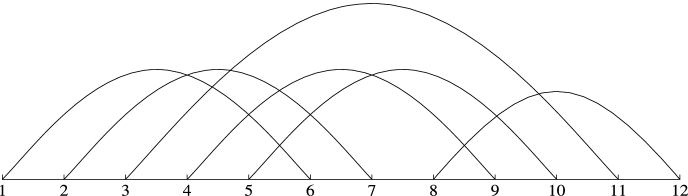
Let $\mathcal{M}_{n}$ be the set of complete matchings of $[2n]$ . The size of $\mathcal{M}_{n}$ is $(2n-1)!!$ . It is well known that the number of complete matchings of $[2n]$ with no crossings equals the $n$ th Catalan number $C_{n}$ , as is the number of complete matchings with no nestings. In 5 , a notation of $r$ -crossing and $r$ -nesting was introduced: given a complete matching $M=\{(i_{1},j_{1}),\ldots,(i_{n},j_{n})\}\in\mathcal{M}_{n}$ , $\{(i_{s_{1}},j_{s_{1}}),\ldots,(i_{s_{r}},j_{s_{r}})\}$ is called an $r$ -crossing if $i_{s_{1}}<i_{s_{2}}<\cdots<i_{s_{r}}<j_{s_{1}}<\cdots<j_{s_{r}}$ and an $r$ -nesting if $i_{s_{1}}<i_{s_{2}}<\cdots<i_{s_{r}}<j_{s_{r}}<\cdots<j_{s_{2}}<j_{s_{1}}$ . Let $\mathrm{cr}_{n}(M)$ be the largest number $k$ such that $M$ has a $k$ -crossing (maximal crossing) and $\mathrm{ne}_{n}(M)$ denote the largest number $j$ such that $M$ has a $j$ -nesting (maximal nesting). See Figure 1 for an example. Various combinatorial properties of $\mathrm{cr}_{n}$ and $\mathrm{ne}_{n}$ were studied by Chen et al. in 5 . This paper subsequently generated a flurry of research concerning crossings and nestings of many combinatorial objects; see, for example, 13 and also the survey article 15 .

Refer to caption — Figure 1: A complete matching $M$ of [12]. In this sample $\mathrm{cr}_{6}(M)=4$ , achieved by $\{(1,6),(2,7),(4,9),(5,10)\}$ , and $\mathrm{ne}_{6}(M)=2$ , achieved by $\{(3,11),(4,9)\}$ .

We may equip $\mathcal{M}_{n}$ with the uniform probability and regard $\mathrm{cr}_{n}$ and $\mathrm{ne}_{n}$ as random variables. Let $\mathcal{N}$ be a Poisson random variable with parameter $t^{2}/2$ and consider matchings of random size distributed as $2\mathcal{N}$ . Let $\mathrm{CR}_{t}$ and $\mathrm{NE}_{t}$ denote $\mathrm{cr}_{\mathcal{N}}$ and $\mathrm{ne}_{\mathcal{N}}$ , respectively. The object of this paper is to study the asymptotics of $\mathrm{CR}_{t}$ and $\mathrm{NE}_{t}$ as $t\to\infty$ .

One of the main results of 5 is that the joint distribution of $\mathrm{cr}_{n}$ and $\mathrm{ne}_{n}$ are symmetric. Hence $\mathrm{CR}_{t}$ and $\mathrm{NE}_{t}$ are symmetrically distributed. The limit of the marginal distribution of $\mathrm{NE}_{t}$ can be obtained by noting a bijection between matchings and fixed-point-free involutions. Let $\operatorname{Inv}_{n}$ be the set of permutations of size $2n$ consisting of only 2-cycles. To $\sigma\in\operatorname{Inv}_{n}$ whose cycles are $(i_{1},j_{1}),\ldots,(i_{n},j_{n})$ , associate the complete matching $\{(i_{1},j_{1}),\ldots,(i_{n},j_{n})\}$ . This gives a natural bijection $\varphi$ from $\operatorname{Inv}_{n}$ onto $\mathcal{M}_{n}$ . Moreover, if we define $\tilde{\ell}_{n}(\sigma)$ as the length of the longest decreasing subsequence of $\sigma\in\operatorname{Inv}_{n}$ , it is easy to check that $\tilde{\ell}_{n}(\sigma)/2=\mathrm{ne}_{n}(\varphi(\sigma))$ . The limiting distribution of $\tilde{\ell}_{n}$ , and also of $\tilde{\ell}_{\mathcal{N}}$ were obtained obtained earlier in 2 , 3 . From this and the symmetry of $\mathrm{cr}_{n}$ and $\mathrm{ne}_{n}$ , Chen et al. 5 concluded that for each $x\in\mathbb{R}$ ,

\lim_{n\to\infty}\mathbb{P}\biggl{\{}\frac{\mathrm{cr}_{n}-\sqrt{2n}}{2^{-1}(2n)^{1/6}}\leq x\biggr{\}}=\lim_{n\to\infty}\mathbb{P}\biggl{\{}\frac{\mathrm{ne}_{n}-\sqrt{2n}}{2^{-1}(2n)^{1/6}}\leq x\biggr{\}}=F(x),

(1)

where $F(x)$ is the GOE Tracy–Widom distribution function from random matrix theory 16 defined in (3) below. We also find a similar result for the Poissonized version,

\lim_{t\to\infty}\mathbb{P}\biggl{\{}\frac{\mathrm{CR}_{t}-t}{2^{-1}t^{1/3}}\leq x\biggr{\}}=\lim_{t\to\infty}\mathbb{P}\biggl{\{}\frac{\mathrm{NE}_{t}-t}{2^{-1}t^{1/3}}\leq x\biggr{\}}=F(x).

(2)

We note that the length $\ell_{n}(\sigma)$ of the longest increasing subsequence of $\sigma\in\operatorname{Inv}_{n}$ has a different distribution from $\tilde{\ell}_{n}$ . For example, while $\tilde{\ell}_{n}(\sigma)$ is always an even integer, $\ell_{n}(\sigma)$ can be both even or odd integers. Moreover, it was shown in 3 that $\frac{\ell_{n}/2-\sqrt{2n}}{2^{-1}(2n)^{1/6}}$ converges to a random variable whose distribution function is different from $F$ ; it is given by the so-called GSE Tracy–Widom distribution. Hence the joint distribution of $\mathrm{cr}_{n}$ and $\mathrm{ne}_{n}$ cannot be the joint distribution of $\ell_{n}/2$ and $\tilde{\ell}_{n}/2$ .

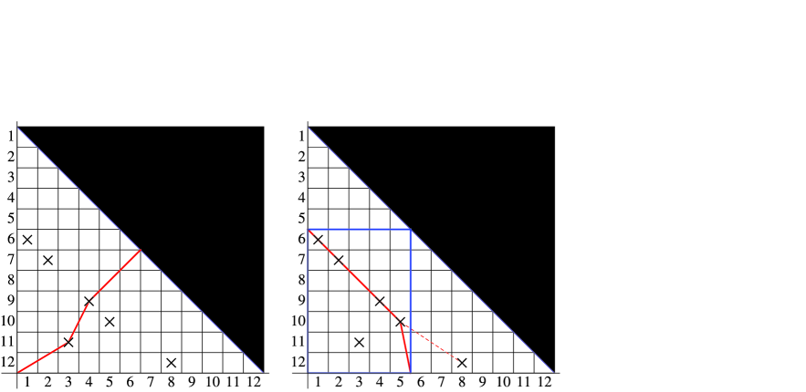
A geometric meaning of $\mathrm{cr}_{n}(\varphi(\sigma))$ and $\mathrm{ne}_{n}(\varphi(\sigma))$ is the following. Represent $\sigma$ as a permutation matrix. Geometrically we imagine the square of size $2n$ with $(1,1)$ entry at the top left corner. The condition that $\sigma$ consists of only 2-cycles implies that the matrix is symmetric and the diagonal entries are zeros. Then it is easy to see that $\mathrm{ne}_{n}(\varphi(\sigma))=\tilde{\ell}_{n}(\sigma)/2$ equals the length of the longest up/right chain consisting of $1$ ’s in the lower-triangle $\{(i,j)\dvtx 1\leq j<i\leq 2n\}$ . On the other hand, for each $k=1,\ldots,2n$ , let $\ell_{n}^{k}(\sigma)$ denotes the length of the longest down/right chain consisting of $1$ ’s in the rectangle with two opposite corners $(2n,1)$ , $(k,k)$ . Then $\mathrm{cr}_{n}(\varphi(\sigma))$ equals the maximum of $\ell_{n}^{k}(\sigma)$ over $k=1,\ldots,2n$ 13 ; see Figure 2.

1.1 Joint distribution

The first main result of this paper is the following result for the joint distribution of $\mathrm{CR}_{t}$ and $\mathrm{NE}_{t}$ . Let $F(x)$ denote the GOE Tracy–Widom distribution defined by

F(x):=\exp\biggl{[}\frac{1}{2}\int_{x}^{\infty}\bigl{(}u(s)-q(s)\bigr{)}\,ds\biggr{]},\qquad u(x):=\int_{\infty}^{x}q(s)^{2}\,ds,

(3)

where $q(s)$ is the unique solution of Painlevé II, $q^{\prime\prime}(s)=sq(s)+q(s)^{3}$ , such that $q(s)\sim\operatorname{Ai}(s)$ as $s\to\infty$ (where $\operatorname{Ai}$ denotes the Airy function). The solution $q(s)$ is called the Hastings–McLeod solution HM ; see also FIK .

Theorem 1.1.

Set

\tilde{\mathrm{CR}}_{t}:=\frac{\mathrm{CR}_{t}-t}{2^{-1}t^{1/3}},\qquad\tilde{\mathrm{NE}}_{t}=\frac{\mathrm{NE}_{t}-t}{2^{-1}t^{1/3}}.

(4)

We have

	$\displaystyle\mathbb{P}\bigl{\{}\tilde{\mathrm{CR}}_{t}\leq x,\tilde{\mathrm{NE}}_{t}\leq x^{\prime}\bigr{\}}$
			(5)
	$\displaystyle\qquad=\mathbb{P}\{\tilde{\mathrm{CR}}_{t}<x\}\mathbb{P}\bigl{\{}\tilde{\mathrm{NE}}_{t}<x^{\prime}\bigr{\}}+\frac{F^{\prime}(x)F^{\prime}(x^{\prime})}{t^{2/3}}+\mathcal{O}\bigl{(}t^{-1}\bigr{)}.$

This, together with a tail estimate, implies the asymptotics of the covariance.

Corollary 1.1.

The covariance of $\mathrm{CR}_{t}$ and $\mathrm{NE}_{t}$ satisfies

\operatorname{Cov}(\mathrm{CR}_{t},\mathrm{NE}_{t})=\tfrac{1}{4}+\mathcal{O}\bigl{(}t^{-1/3}\bigr{)}.

(6)

Hence, the correlation is asymptotically

\rho(\mathrm{CR}_{t},\mathrm{NE}_{t})=\frac{1}{\sigma^{2}t^{2/3}}+\mathcal{O}\bigl{(}t^{-1}\bigr{)},

(7)

where $\sigma^{2}=1.6077810345\ldots$ is the variance of $F(x)$ ; cf. page 862 of Bornemann .

We can also interpret $\mathrm{CR}_{t}$ and $\mathrm{NE}_{t}$ as “height” and “depth” of certain nonintersecting random walks. See Section 2 below.

Table 1: The exact correlation and covariance of

\mathrm{cr}_{n}

and

\mathrm{ne}_{n}

for complete matchings of

[2n]

for the first few nontrivial

n

’s. Note that both statistics are strictly negative

$\bolds{[2n]}$	$\bolds{\#\mathcal{M}_{n}}$	$\bolds{\operatorname{Cov}(\mathrm{cr}_{n},\mathrm{ne}_{n})}$	$\bolds{\operatorname{Cor}(\mathrm{cr}_{n},\mathrm{ne}_{n})}$
4	000003	$-1/9$	$-1/$ 2
6	000015	$-0.137777777$	$-0.418918919$
8	000105	$-0.129614512$	$-0.362983698$
10	000945	$-0.132998516$	$-0.331342276$
12	010395	$-0.143259767$	$-0.309871555$
14	135135	$-0.151180948$	$-0.29369603$ 2

We may apply the de-Poissonization argument 10 to (1.1) to find a result for the joint distribution of $\mathrm{cr}_{n}$ and $\mathrm{ne}_{n}$ . However, intuitively, for fixed $n$ and $M\in\mathcal{M}_{n}$ , any $(i,j)\in M$ that is used to form the maximal crossing of $M$ cannot be used for the maximal nesting of $M$ . This indicates a negative correlation of $\mathrm{cr}_{n}$ and $\mathrm{ne}_{n}$ for a fixed $n$ , contrary to the positive correlation of $\mathrm{CR}_{t}$ and $\mathrm{NE}_{t}$ found in the above corollary. This is verified for small $n$ by direct computation: Table 1 shows exact calculation of the covariance and correlation of $\mathrm{cr}_{n}$ and $\mathrm{ne}_{n}$ for small values of $n$ . For large $n$ , a sampling of 5000 pseudo-random matchings of $[5000]$ yielded the sample covariance of $\tilde{\mathrm{cr}}_{2500}$ and $\tilde{\mathrm{ne}}_{2500}$ equal to $-0.0420258\ldots.$ Therefore, a naive substitution of $t$ by $\sqrt{2n}$ in (1.1) only yields the following weaker result. A further analysis is needed to obtain the correction terms in the asymptotic behavior of $\mathrm{cr}_{n}$ and $\mathrm{ne}_{n}$ . A heuristic explanation for the positive correlation of the Poissonized random matchings is that when $\mathrm{CR}_{t}$ is large, it most likely due to fact that the size of the matching is large, and hence the maximal nesting of the matching is also likely to be large.

Corollary 1.2.

Set

\tilde{\mathrm{cr}}_{n}:=\frac{\mathrm{cr}_{n}-\sqrt{2n}}{2^{-1}(2n)^{1/6}},\qquad\tilde{\mathrm{ne}}_{n}=\frac{\mathrm{ne}_{n}-\sqrt{2n}}{2^{-1}(2n)^{1/6}}.

(8)

For each $x,x^{\prime}\in\mathbb{R}$ ,

\mathbb{P}\bigl{\{}\tilde{\mathrm{cr}}_{n}\leq x,\tilde{\mathrm{ne}}_{n}\leq x^{\prime}\bigr{\}}=\mathbb{P}\{\tilde{\mathrm{cr}}_{n}<x\}\mathbb{P}\bigl{\{}\tilde{\mathrm{ne}}_{n}<x^{\prime}\bigr{\}}+\mathcal{O}\biggl{(}\frac{\sqrt{\log n}}{n^{1/6}}\biggr{)}.

(9)

We compare Theorem 1.1 with the result of Bornemann10 on the joint distribution of the extreme eigenvalues of Gaussian unitary ensemble (GUE). Let $\lambda_{\max}^{(n)}$ and $\lambda_{\min}^{(n)}$ denote the largest and the smallest eigenvalues of $n\times n$ GUE. Setting

\quad\tilde{\lambda}_{\max}^{(n)}:=2^{1/2}n^{1/6}\bigl{(}\lambda_{\max}^{(n)}-\sqrt{2n}\bigr{)},\qquad\tilde{\lambda}_{\min}^{(n)}:=2^{1/2}n^{1/6}\bigl{(}\lambda_{\min}^{(n)}+\sqrt{2n}\bigr{)},

(10)

it was shown in Bornemann10 that

	$\displaystyle\mathbb{P}\bigl{\{}\tilde{\lambda}_{\max}^{(n)}\leq x,\tilde{\lambda}_{\min}^{(n)}\leq x^{\prime}\bigr{\}}$
			(11)
	$\displaystyle\qquad=\mathbb{P}\bigl{\{}\tilde{\lambda}_{\max}^{(n)}<x\bigr{\}}\mathbb{P}\bigl{\{}\tilde{\lambda}_{\min}^{(n)}<x^{\prime}\bigr{\}}+\frac{F_{\mathrm{GUE}}^{\prime}(x)F_{\mathrm{GUE}}^{\prime}(x^{\prime})}{4n^{2/3}}+\mathcal{O}\bigl{(}n^{-4/3}\bigr{)},$

where $F_{\mathrm{GUE}}$ is the GUE Tracy–Widom distribution function defined by

F_{\mathrm{GUE}}(x):=\exp\biggl{[}\int_{x}^{\infty}u(s)\,ds\biggr{]}.

(12)

It is interesting to study the joint distribution of the extreme eigenvalues of Gaussian orthogonal ensemble (GOE) and compare the result with (1.1). This will be done in a separate paper. It might also be interesting to see if the error term of (1.1) can be improved to $\mathcal{O}(t^{-4/3})$ as in (1.1), but we do not pursue this in this paper.

1.2 Marginal distribution

We also evaluate the second order term in the asymptotics expansion of the marginal distributions of $\mathrm{CR}_{t}$ and $\mathrm{NE}_{t}$ explicitly. Let $[a]$ denote the largest integer less than or equal to $a$ .

Theorem 1.2.

For $x\in\mathbb{R}$ and $t>0$ , define $x_{t}$ by

x_{t}:=\frac{[t+2^{-1}xt^{1/3}]-t}{2^{-1}t^{1/3}}+\frac{1}{t^{1/3}}.

(13)

For each $x\in\mathbb{R}$ ,

	$\displaystyle\mathbb{P}\{\tilde{\mathrm{CR}}_{t}\leq x\}$	$\displaystyle=$	$\displaystyle\mathbb{P}\{\tilde{\mathrm{NE}}_{t}\leq x\}$
		$\displaystyle=$	$\displaystyle F(x_{t})-\frac{1}{20t^{2/3}}\biggl{[}4F^{\prime\prime}(x)+\frac{1}{3}x^{2}F^{\prime}(x)\biggr{]}+\mathcal{O}\bigl{(}t^{-1}\bigr{)}.$

Note that since $\mathbb{P}\{\mathrm{CR}_{t}\leq x\}$ has the same value for $x\in[\ell,\ell+1)$ for a given integer $\ell$ , it is natural that the leading term $F(x_{t})$ of (194) is expressed in terms of $x_{t}$ , which contains $[t+2^{-1}xt^{1/3}]$ .

In addition to this integral part correction, there is an additional shift by $t^{-1/3}$ from $x$ in the definition of $x_{t}$ . This is responsible for the absence of the term of order $t^{-1/3}$ in the expansion (194). For classical ensembles in random matrix theory, there are several papers that showed that a fine scaling can remove such a term (which looks like a natural term to be present.) See ElKaroui for the Laguerre unitary ensemble, Johnstone for Jacobi unitary and orthogonal ensembles, Ma for the Laguerre orthogonal ensemble and JohnstoneMa for Gaussian unitary and orthogonal ensembles. A similar result was obtained recently for random growth models and intersecting particle systems in FerrariFrings , including the height of the so-called PNG model with flat initial condition. It is well known that this is precisely the length of the longest decreasing subsequence of random fixed-point-free involution and hence $\mathrm{NE}_{t}$ . The result of FerrariFrings in the context of this paper is that $\mathbb{P}\{\tilde{\mathrm{NE}}_{t}\leq x\}=F(x_{t})+O(t^{-2/3})$ . The above result finds the term of order $O(t^{-2/3})$ explicitly.

As in the joint distribution, the evaluation of the second order term of $\mathbb{P}\{\tilde{\mathrm{cr}}_{n}\leq x\}$ does not immediately follow from the de-Poissonization argument in 10 . It remains an open problem to evaluate the the error terms of $\mathbb{P}\{\tilde{\mathrm{cr}}_{n}\leq x\}$ asymptotically.

1.3 Toeplitz minus Hankel with a discrete symbol

Set

G_{k,j}(t):=\sum_{n=0}^{\infty}g_{k,j}(n)\frac{t^{2n}}{(2n)!},

(15)

where $g_{k,j}(n):=\#\{M\in\mathcal{M}_{n}\dvtx\mathrm{cr}_{n}(M)\leq k,\mathrm{ne}_{n}(M)\leq j\}$ so that

	$\displaystyle\mathbb{P}\{\mathrm{CR}_{t}\leq k,\mathrm{NE}_{t}\leq j\}$	$\displaystyle=$	$\displaystyle\sum_{n=0}^{\infty}\mathbb{P}\{\mathrm{cr}_{\mathcal{N}}\leq k,\mathrm{ne}_{\mathcal{N}}\leq j\|\mathcal{N}=n\}\mathbb{P}\{\mathcal{N}=n\}$
		$\displaystyle=$	$\displaystyle e^{-t^{2}/2}G_{k,j}(t).$

An explicit determinantal formula of $G_{k,j}(t)$ was obtained in 5 which we describe now.

Stanley had shown earlier that matchings are in bijection with oscillating tableaux of empty shape and of length $2n$ ; see Section 5 of 5 . This was further generalized to a bijection between partitions of a set and so-called vacillating tableaux in 5 . In the same paper, it was shown that the maximal crossing (resp., nesting) of a partition equals the maximal number of rows (resp., columns) in any partitions appearing in the corresponding vascillating tableau.

Since an oscillating tableau can be thought of as a walk in the chamber of the affine Weyl group $\tilde{C}_{n}$ , $g_{k,j}(n)$ equals the number of walks with $n$ steps from $(j,j-1,\ldots,2,1)$ to itself in the chamber $0<x_{j}<\cdots<x_{2}<x_{1}<j+k+1$ where each step is a unit coordinate vector or its negative in $\mathbb{Z}^{j}$ . The number of such walks was evaluated by Grabnier in 9 using the Gessel–Viennot method of evaluation of nonintersecting paths. This result implies (see the displayed equation before (5.3) in 5 ) that

G_{k,j}(t)=\det\Biggl{[}\frac{1}{m}\sum_{r=0}^{2m-1}\sin\biggl{(}\frac{\pi ra}{m}\biggr{)}\sin\biggl{(}\frac{\pi rb}{m}\biggr{)}e^{2t\cos(\pi r/m)}\Biggr{]}_{a,b=1}^{j},

(17)

where

m:=j+k+1.

(18)

We prove Theorem 1.1 by analyzing the determinant (17) asymptotically. For this purpose, we first re-formulate the determinant slightly. By writing the product of the sine functions in terms of a sum of two cosine functions and noting the realness of the entries, we find that

G_{k,j}(t)=\det[h_{a-b}-h_{a+b}]_{a,b=1}^{j},

(19)

where

h_{\ell}:=\frac{1}{2m}\sum_{r=0}^{2m-1}e^{-i\pi r\ell/m}e^{2t\cos(\pi r/m)}.

(20)

This is the determinant of a Toeplitz matrix minus a Hankel matrix. This structure is important in the asymptotic analysis. An interesting feature of the above determinant is that the measure for the Toeplitz determinant is not an absolutely continuous measure but a discrete measure.

Let $\omega:=e^{\pi i/m}$ be the primitive $2m$ th root of unity. Define the discrete measure

d\mu_{m}(z):=\frac{1}{2m}\sum_{r=0}^{2m-1}e^{t(z+z^{-1})}\delta_{\omega^{r}}(z)

(21)

on the circle. Let $\pi_{n,m}(z)$ be the monic orthogonal polynomial of degree $n$ with respect to $d\mu_{m}$ , defined by the conditions

\oint_{|z|=1}z^{-\ell}\pi_{n,m}(z)\,d\mu_{m}(z)=0,\qquad 0\leq\ell<n.

(22)

We emphasize the dependence on $m$ since later we will use the notation $\pi_{n,\infty}$ to denote the case when “ $m=\infty$ ;” the orthogonal polynomials with respect to the absolutely continuous measure $e^{t(z+z^{-1})}\frac{dz}{2\pi iz}$ . Note that $d\mu_{m}$ depends on the parameter $t$ and hence $\pi_{n,m}(z)$ also depends on $t$ . When we wish to emphasize this dependence on $t$ , we write $\pi_{n,m}(z;t)$ .

The fact that the $t$ -dependence of the measure is from the factor $e^{t(z+z^{-1})}$ implies the following basic formula, which is proved in Section 3 below. Recall from (18) that $m:=j+k+1$ .

Proposition 1.1.

We have

	$\displaystyle\log\mathbb{P}\{\mathrm{CR}_{t}\leq k,\mathrm{NE}_{t}\leq j\}$
			(23)
	$\displaystyle\qquad=\int_{0}^{t}\pi_{2j+1,m}(0;\tau)\,d\tau+\int_{0}^{t}\int_{0}^{s}\mathcal{Q}_{j}^{m}(\tau)\,d\tau\,ds,$

where

	$\displaystyle\mathcal{Q}_{j}^{m}(\tau)$	$\displaystyle:=$	$\displaystyle-\bigl{(}\pi_{2j,m}(0;\tau)\pi_{2j+2,m}(0;\tau)+\bigl{\|}\pi_{2j+1,m}(0;\tau)\bigr{\|}^{2}\bigr{)}$
			$\displaystyle{}+\pi_{2j,m}(0;\tau)\pi_{2j+2,m}(0;\tau)\bigl{\|}\pi_{2j+1,m}(0;\tau)\bigr{\|}^{2}.$

We obtain the asymptotics $\pi_{2j+\ell,m}(0,\tau)$ for $\ell=0,1,2$ by using the associated discrete version of the Riemann–Hilbert problem; see, for example, BKMM . See Sections 4, 5 and 6 below.

We compare the analysis of this paper based on the formula (1.1) with the analysis of the determinant of a similar Toeplitz minus Hankel matrix in 3 . Even though the determinant in 3 was for continuous measure (which is precisely the one for the marginal distribution of $\mathrm{NE}_{t}$ ; see Section 3 below), the basic structure of the matrix is the same; a Toeplitz minus a Hankel matrix. Denoting the matrix by $D_{j}$ , the approach of 3 was to write $D_{j}=D_{\infty}\prod_{n=j}^{\infty}\frac{D_{n}}{D_{n+1}}$ where $D_{\infty}$ is the strong Szegö limit, which exists in that particular case, and analyze $D_{n}/D_{n+1}$ , which can be evaluated from the Riemann–Hilbert problem for the $n$ th orthogonal polynomial. For our case, since the measure is discrete, the strong Szegö limit does not apply. Indeed $D_{n}=0$ for all large enough $n$ . Then alternatively one can still analyze $D_{j}$ by expressing $D_{j}=D_{0}\prod_{n=1}^{j}\frac{D_{n}}{D_{n-1}}$ as was done in BBD . However, this expression is more subtle to analyze since $\log(D_{n}/D_{n+1})$ is not small when $n$ is small (indeed it grows as $n$ decreases when $t$ is proportional to $j$ ) and this requires careful cancellations of the terms in the product. Though this was done for the leading term in BBD , the evaluation of the lower terms in the asymptotic expansion in this method becomes more complicated. A particularly useful point in using formula (1.1) is that we only need to consider the so-called full band case (and the transitional case when a gap and a saturated region are about to open up) in the Riemann–Hilbert analysis. This makes the analysis much simpler, and it becomes easier to evaluate the lower order terms. On the contrary, if we use the expression $D_{j}=D_{0}\prod_{n=1}^{j}\frac{D_{n}}{D_{n-1}}$ , then we need to consider both the so-called void-band case and the saturation-band case, including the transitional cases, in the Riemann–Hilbert analysis (and this is the reason for the need of cancellations mentioned above.)

The continuous Riemann–Hilbert problem for $\pi_{n,\infty}(z;t)$ was analyzed asymptotically to the leading term in BDJ , 2 , BBD . We expand this work to the discrete counterpart and moreover, we improve the analysis so that we compute explicit formulae for the first three terms in the expansion of the solution in both the discrete and continuous cases. As a technical note, we remark that we use a different local map for the so-called Painlevé parametrix related to the local problem for the Riemann–Hilbert problem from the previous cases BDJ , CK . We adapt the map used in the recent paper BMiller for a different parametrix, which seems to be useful for further analysis in other Riemann–Hilbert problems. For the purpose of this paper, we only analyze the full band case (and the transitional case) of the discrete Riemann–Hilbert problem. The analysis for the full parameter set of the discrete Riemann–Hilbert problem will be discussed somewhere else in the context of Ablowitz–Ladik equations and Schur flows in integrable systems.

A determinantal formula of the marginal distribution $\mathbb{P}\{\mathrm{NE}_{t}\leq j\}$ can be obtained from the joint distribution by taking $k\to\infty$ while keeping $j$ fixed. Then we find a Toeplitz minus a Hankel determinant with symbol $e^{t(z+z^{-1})}$ . Here too, the factor of $e^{t(z+z^{-1})}$ in the limiting measure implies a formula for the marginal distribution analogous to (1.1). See Section 3 below.

The Toeplitz determinant with symbol $e^{t(z+z^{-1})}$ is known to be describe the distribution of the length of the longest increasing subsequence of a random permutation Gessel . By using a formula similar to (1.1), the analysis of this paper implies the following result.

1.4 Longest increasing subsequence of random permutation

Consider the symmetric group $S_{n}$ of permutations of size $n$ and equip it with the uniform probability. Let $l_{n}(\pi)$ denote the length of the longest increasing subsequence of $\pi\in S_{n}$ . Let $\mathcal{N}_{1}$ be a Poisson random variable with parameter $t^{2}$ and let $L_{t}$ denotes $l_{\mathcal{N}_{1}}$ . It was shown in BDJ that $\frac{L_{t}-2t}{t^{1/3}}$ converges to the GUE Tracy–Widom distribution (12). We evaluate the next term of the asymptotic expansion explicitly.

Theorem 1.3.

For each $x\in\mathbb{R}$ ,

	$\displaystyle\mathbb{P}\biggl{\{}\frac{L_{t}-2t}{t^{1/3}}\leq x\biggr{\}}$
			(25)
	$\displaystyle\qquad=F_{\mathrm{GUE}}\bigl{(}x^{(t)}\bigr{)}-\frac{1}{10t^{2/3}}\biggl{[}F_{\mathrm{GUE}}^{\prime\prime}(x)+\frac{1}{6}x^{2}F_{\mathrm{GUE}}^{\prime}(x)\biggr{]}+\mathcal{O}\bigl{(}t^{-1}\bigr{)},$

where

x^{(t)}:=\frac{[2t+xt^{1/3}]-2t}{t^{1/3}}.

(26)

The study in FerrariFrings also considered the height of the so-called PNG model with the droplet initial condition, which is distributed precisely as $L_{t}$ , and showed that the above distribution function is $F_{\mathrm{GUE}}(x^{(t)})+O(t^{-2/3})$ . The above theorem evaluates the error term explicitly.

For the Gaussian unitary ensemble, Choup Choup2006 , Choup2008 evaluated the distribution of the largest eigenvalue explicitly up to the term of order $O(n^{-2/3})$ which corresponds to the term of order $t^{-2/3}$ in the above expansion. It would be interesting to compare the term in the above theorem with the formula of Choup2006 , Choup2008 .

1.5 Organization of paper

In Section 2, we consider a nonintersecting random process that gives rise to $\mathrm{CR}_{t}$ and $\mathrm{NE}_{t}$ . Proof of Proposition 3 is given in Section 3. The Riemann–Hilbert problem is introduced in Section 4, and is analyzed asymptotically in Sections 5 and 6. Theorem 1.1 and Corollary 1.1 are proved in Secton 7, and Theorems 1.2 and 1.3 are proved in Section 8. We prove Corollary 1.2 in Section 9 using a de-Poissonization argument. Finally, the Riemann–Hilbert problem for the Painlevé II equations that are needed to model the local parametrix of the Riemann–Hilbert problem for orthogonal polynomials are discussed in Section 10.

2 Height and depth of nonintersecting continuous-time simple random walks

In Section 1.3 we discussed a relation between $\mathrm{cr}_{n}$ and $\mathrm{ne}_{n}$ and a walk in the chamber $\{0<x_{j}<\cdots<x_{2}<x_{1}<j+k+1\}$ of the affine Weyl group $\tilde{C}_{n}$ . In this section, we give an interpretation of $\mathrm{CR}_{t}$ and $\mathrm{NE}_{t}$ in terms of the “height” and “depth” of continuous-time simple random walks.

Let $N^{+}(\tau)$ and $N^{-}(\tau)$ be two independent Poisson processes of rate 1 and let $Z(\tau):=N^{+}(\tau)-N^{-}(\tau)$ be a continuous-time simple random walk. Then $Z(\tau)$ is an $\mathbb{Z}$ -valued Markov process with the transition probability $p_{s}(a,b)=p_{s}(a-b)$ where $p_{t}(a)=e^{-2t}\sum_{n\in\mathbb{Z}}\frac{t^{2n+a}}{n!(n+a)!}=p_{t}(-a)$ for $a\in\mathbb{Z}$ . Here we used the convention that $1/n!\equiv 0$ if $n<0$ . Set

\phi(z):=\sum_{a\in\mathbb{Z}}\bigl{(}e^{-2t}p_{t}(a)\bigr{)}z^{-a}=e^{t(z+z^{-1})}.

(27)

Then we have

p_{t}(a)=e^{-2t}\phi_{-a}=e^{-2t}\phi_{a},\qquad\phi_{a}:=\oint_{|z|=1}z^{-a}\phi(z)\frac{dz}{2\pi iz}.

(28)

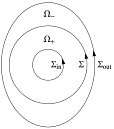
Let $Z_{i}(\tau),i=0,1,2,\ldots,$ be independent copies of $Z(\tau)$ , and consider the infinite system of processes $X_{i}(\tau)=Z_{i}(\tau)-i,i=0,1,2,\ldots.$ Fix a number $t>0$ . We will consider the process conditioned on the event that (a) $X_{i}(t)=X_{i}(0)$ for all $i$ and (b) $X_{i}(\tau)$ do not intersect in time $[0,t]$ , that is, $X_{0}(\tau)>X_{1}(\tau)>\cdots$ for all $\tau\in[0,t]$ . A precise interpretation will be given below. Such nonintersecting continuous-time simple random walks have been studied, for example, in OConnell02 , 1 , AdlerFvM .

Define the “height” $K:=\max_{\tau\in[0,t]}X_{0}(\tau)$ and define the “depth” $J$ as the smallest index such that $X_{i}(\tau)=i$ for all $\tau\in[0,t]$ and for all $i=J,J+1,\ldots,$ in other words, only the top $J$ processes moved in the interval $[0,t]$ . We are interested in the joint distribution of $J$ and $K$ conditional of the above event satisfying (a) and (b).

Precisely, fix $N\in\mathbb{N}$ and let $\mathfrak{A}_{N}$ and $\mathfrak{B}_{N}$ be the events defined as

	$\displaystyle\mathfrak{A}_{N}$	$\displaystyle:=$	$\displaystyle\bigl{\{}X_{i}(t)=X_{i}(0)=-i,i=0,1,\ldots,N-1\bigr{\}},$		(29)
	$\displaystyle\mathfrak{B}_{N}$	$\displaystyle:=$	$\displaystyle\bigl{\{}X_{0}(\tau)>X_{1}(\tau)>\cdots>X_{N-1}(\tau)\geq-N+1,\tau\in[0,t]\bigr{\}}.$		(30)

The condition that $X_{N-1}(\tau)\geq-N+1$ for all $\tau\in[0,t]$ is natural because $J$ is likely to be a finite number and by definition of $J$ , $X_{J-1}(\tau)\geq X_{J-1}(0)$ for all $\tau\in[0,t]$ . The joint distribution of $K$ and $J$ is interpreted as

P(k,j):=\lim_{N\to\infty}\mathbb{P}(K\leq k,J\leq j|\mathfrak{A}_{N}\cap\mathfrak{B}_{N}).

(31)

Lemma 2.1.

Let $K$ and $J$ be the “height” and “depth,” respectively, defined above. Then

P(k,j)=e^{-t^{2}/2}G_{k,j}(t),

(32)

where $G_{k,j}(t)$ is given in (19).

{pf}

We first evaluate $\mathbb{P}(\mathfrak{A}_{N}\cap\mathfrak{B}_{N})$ . The condition that $X_{i}(\tau)>-N$ , $i=0,\ldots,N-1$ , implies that $X_{i}(\tau)$ has an absorbing boundary at $-N$ . Since the transition probability of $X_{i}$ with an absorbing boundary at $-N$ is $p_{t}(a,b)-p_{t}(-2N-a,b)$ , the Karlin–McGregor formula 11 of nonintersecting probability applied to continuous-time simple random walks (see, e.g., AdlerFvM , 1 ) implies then that

	$\displaystyle\mathbb{P}(\mathfrak{A}_{N}\cap\mathfrak{B}_{N})$	$\displaystyle=$	$\displaystyle\det\bigl{[}p_{t}(-a,-b)-p_{t}(-2N+a,-b)\bigr{]}_{a,b=0}^{N-1}$
		$\displaystyle=$	$\displaystyle e^{-2tN}\det[\phi_{a-b}-\phi_{a+b}]_{a,b=1}^{N}.$

Second, we evaluate $\mathbb{P}(\{K\leq k,J\leq j\}\cap\mathfrak{A}_{N}\cap\mathfrak{B}_{N})$ . We assume that $N$ is large so that $N\geq j$ . By the definition of $K$ and $J$ , the desired probability equals $\mathbb{P}(\mathfrak{C}\cap\mathfrak{D})$ where $\mathfrak{C}$ and $\mathfrak{D}$ are independent events defined as follows. $\mathfrak{C}$ is the event that the top $j$ processes, $X_{0}(\tau),\ldots,X_{j-1}(\tau)$ , satisfy the two conditions (a) $X_{i}(t)=X_{i}(0)$ for all $i=0,\ldots,j-1$ and (b) $-j+1\leq X_{j-1}(\tau)<\cdots<X_{0}(\tau)\leq k$ for all $\tau\in[0,t]$ , that is, the $j$ nonintersecting paths are not absorbed at the boundaries $-j$ and $k+1$ . $\mathfrak{D}$ is the event that $X_{i}(\tau)=-i$ for all $i=j,j+1,\ldots,N-1$ and for all $\tau\in[0,t]$ , that is, the bottom $N-j$ processes stay put during the interval $[0,t]$ . Clearly, $\mathbb{P}(\mathfrak{D})=(e^{-2t})^{N-j}$ . On the other hand, from the Karlin–McGregor formula again, $\mathbb{P}(\mathfrak{C})=\det[\hat{p}_{t}(-a,-b)]_{a,b=0}^{j-1}$ where $\hat{p}_{t}(a,b)$ is the transition probability of $Z(\tau)$ in the presence of the absorbing walls at $-j$ and $k+1$ in time $t$ . It is easy to see that

\hat{p}_{t}(a,b)=\sum_{n\in\mathbb{Z}}\bigl{[}p_{t}(a+2nm,b)-p_{t}(-2j-a+2nm,b)\bigr{]},

(34)

where $m:=j+k+1$ . Now consider the identity $z^{-a}\phi(z)=\sum_{n\in\mathbb{Z}}\phi_{a+n}z^{n}$ . Set $\omega:=e^{\pi i/m}$ . By inserting $z=\omega^{r}$ , $r=0,1,\ldots,2m-1$ and summing over $r$ , we find that

\sum_{r=0}^{2m-1}\bigl{(}\omega^{r}\bigr{)}^{-a}\phi\bigl{(}\omega^{r}\bigr{)}=2m\sum_{n\in\mathbb{Z}}\phi_{a+2mn},\qquad\omega:=e^{\pi i/m}.

(35)

Hence from (28), (34) becomes

\hat{p}_{t}(a,b)=e^{-2t}(h_{a-b}-h_{-a-b+2j}),

(36)

where

h_{a}:=\oint_{|z|=1}z^{-a}\,d\mu_{m}(z),\qquad d\mu_{m}(z):=\frac{1}{2m}\sum_{r=0}^{2m-1}\phi(z)\delta_{\omega^{r}}(z).

(37)

Hence, for $N\geq j$ ,

\mathbb{P}\bigl{(}\{K\leq k,J\leq j\}\cap\mathfrak{A}_{N}\cap\mathfrak{B}_{N}\bigr{)}=e^{-2tN}\det[h_{a-b}-h_{a+b}]_{a,b=1}^{j}.

(38)

The strong Szegö limit theorem for Toeplitz minus Hankel determinants (see, e.g., 4 ) implies that for the function $\phi(z)$ in (27), $\det[\phi_{a-b}-\break\phi_{a+b}]_{a,b=1}^{N}\to e^{t^{2}/2}$ as $N\to\infty$ . Therefore, from (2) and (38) we find that

\qquad P(j,k)=\lim_{N\to\infty}\frac{\det[h_{a-b}-h_{a+b}]_{a,b=1}^{j}}{\det[\phi_{a-b}-\phi_{a+b}]_{a,b=1}^{N}}=e^{-t^{2}/2}\det[h_{a-b}-h_{a+b}]_{a,b=1}^{j}.

(39)

This is (32).

Hence $K$ and $J$ have the same joint distribution as $\mathrm{CR}_{t}$ and $\mathrm{NE}_{t}$ . This nonintersecting process interpretation of $\mathrm{CR}_{t}$ and $\mathrm{NE}_{t}$ provides some useful information. As an example, note that the process considered above has a natural dual process; see Figure 3. In the dual process the roles of $K$ and $J$ are reversed: the depth is $K$ and height is $J$ in the dual process. It follows that $K$ and $J$ , and hence $\mathrm{CR}_{t}$ and $\mathrm{NE}_{t}$ , are symmetrically distributed.

In various nonintersecting processes, including the above model, the top curve is shown to converge, after appropriate scaling, to the Airy process in the long-time, many-walker limit; see, for example, Johansson02 , Johansson05 . Then it is natural to think that the leading fluctuation term of $K$ is given by the maximum of the Airy process. It is a well-known fact that the maximum of the Airy process is distributed as the GOE Tracy–Widom distribution. This was first proved indirectly in Johansson03 . A direct proof was only recently obtained in CorwinQR . (See also MFQuastelR for the distribution of the location of the maxima.) Hence the leading term $F(x)$ in (194) is as expected. Moreover, when $t$ becomes large, it is plausible to expect that the fluctuation of the top curve of the original process (whose max is $K$ ) and the fluctuation of the bottom curve of the dual process (whose min is $-J$ ) become independent at least to the leading order. The leading term of Theorem 1.1 is natural from this. Theorem 1.1 evaluates the second term of the asymptotic expansion of their joint distribution.

For a family of finitely many nonintersecting walks, it is interesting to consider the maximum of the top curve and the minimum of the bottom curve. It is curious to check if the joint distribution of them would have the same expansion as in Theorem 1.1. This will be considered elsewhere. Finally, we mention that the asymptotics of the distribution of the width of nonintersecting processes was studied recently in BaikLiu .

3 Proof of Proposition 1.1

In this section, we give a proof of Proposition 1.1. We also obtain similar formulas for the marginal distributions of $\mathrm{CR}_{t}$ and $\mathrm{NE}_{t}$ , and for the distribution of $L_{t}$ . They are stated at the end of this section.

Let $d\rho$ be a (either continuous or discrete) measure on the unit circle and define a new measure $d\rho(z;t)$ which depends on a parameter $t$ as

d\rho(z;t):=e^{t(z+z^{-1})}\,d\rho(z).

(40)

Measure (21), associated to the joint distribution of $\mathrm{CR}_{t},\mathrm{NE}_{t}$ , is certainly of this form, but the following algebraic steps apply to general $d\rho$ .

Let

h_{\ell}(t):=\oint_{|z|=1}z^{-\ell}\,d\rho(z;t).

(41)

We are interested in finding a simple formula for the second derivative of the Toeplitz determinant $T_{n}(t)$ and the Toeplitz–Hankel determinant $H_{n}(t)$ [see (19)] associated to the measure $d\rho(z;t)$ ,

\qquad T_{n}(t):=\det\bigl{[}h_{a-b}(t)\bigr{]}_{a,b=1}^{n},\qquad H_{n}(t)=\det\bigl{[}h_{a-b}(t)-h_{a+b}(t)\bigr{]}_{a,b=1}^{n}.

(42)

We assume that when $d\rho$ is a discrete measure, $n$ is smaller than the number of points in the support of $d\rho$ .

Let $\pi_{n}(z;t)=z^{n}+\cdots,$ $n=0,1,2,\ldots,$ be the monic orthogonal polynomials defined by the conditions

\bigl{\langle}\pi_{n},z^{\ell}\bigr{\rangle}:=\oint_{|z|=1}\pi_{n}(z;t)\overline{z^{\ell}}\,d\rho(z;t)=0,\qquad 0\leq\ell<n.

(43)

Set

N_{n}(t):=\langle\pi_{n},\pi_{n}\rangle=\bigl{\langle}\pi_{n},z^{n}\bigr{\rangle}.

(44)

Then it is well known that (see, e.g., Sections 2 and 3 of 2 for the second identity)

T_{j}(t)=\prod_{n=0}^{j-1}N_{n}(t),\qquad H_{j}(t)=\prod_{n=1}^{j}N_{2n}(t)\bigl{(}1-\pi_{2n}(0;t)\bigr{)}^{-1}.

(45)

Define (see Szego )

\pi^{*}_{n}(z;t):=z^{n}\overline{\pi_{n}\bigl{(}z^{-1};t\bigr{)}}=1+\overline{a_{n-1}}z+\cdots+\overline{a_{1}}z^{n-1}+\overline{\pi_{n}(0;t)}z^{n}.

(46)

This polynomial satisfies the orthogonality properties

\bigl{\langle}{\pi_{n}^{*}},{z^{k}}\bigr{\rangle}=N_{n}\delta_{k,0},\qquad k=0,1,\ldots,n.

(47)

Recall the Szegö recurrence relations Szego ,

	$\displaystyle\pi_{n+1}(z)$	$\displaystyle=$	$\displaystyle z\pi_{n}(z)+\pi_{n+1}(0)\pi^{*}_{n}(z),$
	$\displaystyle z\pi_{n}(z)$	$\displaystyle=$	$\displaystyle\frac{N_{n}}{N_{n+1}}\bigl{(}\pi_{n+1}(z)-\pi_{n+1}(0)\pi_{n+1}^{*}(z)\bigr{)}.$

The second relation, when we compare the coefficients of $z^{n+1}$ , gives rise to the relation

\displaystyle\frac{N_{n+1}}{N_{n}}=1-\bigl{|}\pi_{n+1}(0)\bigr{|}^{2}.

(49)

We now derive differential equations for $\pi_{n}(0;t)$ and $N_{n}(t)$ . All the differentiations are with respect to $t$ , and we use the notation $f^{\prime}$ for $\frac{d}{dt}f$ . By differentiating the formula $\langle{\pi_{n}},{z^{k}}\rangle=0,k=0,\ldots,n-1$ , we obtain, by noting $\frac{{d}}{{d}t}e^{t(z+z^{-1})}=(z+z^{-1})e^{t(z+z^{-1})}$ , that $\langle{\pi_{n}^{\prime}},{z^{k}}\rangle+\langle{\pi_{n}},{z^{k+1}+z^{k-1}}\rangle=0$ . Then by using the orthogonality conditions, we find that

$\displaystyle\bigl{\langle}{\pi_{n}^{\prime}},{z^{k}}\bigr{\rangle}$	$\displaystyle=$	$\displaystyle 0,\qquad k=1,\ldots,n-2,$
$\displaystyle\bigl{\langle}{\pi_{n}^{\prime}},{1}\bigr{\rangle}$	$\displaystyle=$	$\displaystyle-\bigl{\langle}{\pi_{n}},{z^{-1}}\bigr{\rangle}=-\langle{z\pi_{n}},{1}\rangle=\pi_{n+1}(0)N_{n},$	(50)
$\displaystyle\bigl{\langle}{\pi_{n}^{\prime}},{z^{n-1}}\bigr{\rangle}$	$\displaystyle=$	$\displaystyle-\bigl{\langle}{\pi_{n}},{z^{n}}\bigr{\rangle}=-N_{n},$

where the last equality in the second condition above follows from the first recurrence in (3). From these relations, we conclude that, for $n\geq 1$ ,

\pi_{n}^{\prime}(z;t)=\frac{N_{n}(t)}{N_{n-1}(t)}\bigl{(}\pi_{n+1}(0;t)\pi_{n-1}^{*}(z;t)-\pi_{n-1}(z;t)\bigr{)}.

(51)

This can be checked by taking the difference and noting that the difference is a polynomial of degree at most $n-1$ and is orthogonal to $z^{k}$ , $k=0,1,\ldots,n-1$ . Evaluating (51) at $z=0$ , we obtain, using (49), for $n\geq 1$ ,

\pi_{n}^{\prime}(0;t)=\bigl{(}\pi_{n+1}(0;t)-\pi_{n-1}(0;t)\bigr{)}\bigl{(}1-\bigl{|}\pi_{n}(0;t)\bigr{|}^{2}\bigr{)}.

(52)

This equation is related to the Ablowitz–Ladik equations and the Schur flows; see, for example, Nenciu , Golinskii .

We also differentiate $N_{n}(t)=\langle{\pi_{n}},{\pi_{n}}\rangle$ and obtain

\displaystyle N_{n}^{\prime}

\displaystyle=2\bigl{\langle}{\pi_{n}^{\prime}},{\pi_{n}}\bigr{\rangle}+2\langle{z\pi_{n}},{\pi_{n}}\rangle=\langle 2z\pi_{n},\pi_{n}\rangle.

(53)

Using the first recurrence of (3),

\displaystyle\langle{z\pi_{n}},{\pi_{n}}\rangle=\langle{\pi_{n+1}},{\pi_{n}}\rangle-\pi_{n+1}(0)\bigl{\langle}{\pi_{n}},{\pi_{n}^{*}}\bigr{\rangle}=-\pi_{n+1}(0)\pi_{n}(0)\bigl{\langle}{\pi_{n}},{z^{n}}\bigr{\rangle}.

(54)

Hence, we obtain, for $n\geq 0$ ,

N_{n}^{\prime}(t)=-2\pi_{n+1}(0;t)\pi_{n}(0;t)N_{n}(t).

(55)

We now evaluate the logarithmic derivatives of $T_{j}$ and $H_{j}$ . From (45) and (55), we find that

\bigl{(}\log T_{j}(t)\bigr{)}^{\prime}=\sum_{n=0}^{j-1}\frac{N_{n}(t)}{N_{n}(t)}=-2\sum_{n=0}^{j-1}\pi_{n}(0;t)\pi_{n+1}(0;t).

(56)

We take one more derivative. By using (52), for $n\geq 1$ ,

\bigl{(}\pi_{n}(0)\pi_{n+1}(0)\bigr{)}^{\prime}=P_{n+1}-P_{n},

(57)

where $P_{n}:=|\pi_{n}(0)|^{2}+\pi_{n-1}(0)\pi_{n+1}(0)(1-|\pi_{n}(0)|^{2})$ . For $n=0$ , $(\pi_{0}(0)\pi_{1}(0))^{\prime}=\pi_{1}^{\prime}(0)=(\pi_{2}(0)-1)(1-|\pi_{1}(0)|^{2})=P_{1}-1$ . Hence from a telescoping sum, we obtain

	$\displaystyle\tfrac 12\bigl{(}\log\bigl{(}e^{-t^{2}}T_{j}(t)\bigr{)}\bigr{)}^{\prime\prime}$
			(58)
	$\displaystyle\qquad=-\bigl{(}\pi_{j-1}(0)\pi_{j+1}(0)+\bigl{\|}\pi_{j}(0)\bigl{\|}^{2}\bigr{)}+\pi_{j-1}(0)\pi_{j+1}(0)\bigl{\|}\pi_{j}(0)\bigr{\|}^{2}.$

We now consider $H_{j}(t)$ in (45). By taking the log derivative and using (52), (55) and $\pi_{0}(z)=1$ ,

\qquad\bigl{(}\log H_{j}(t)\bigr{)}^{\prime}=\sum_{n=1}^{j}\biggl{[}\frac{N_{2n}^{\prime}}{N_{2n}}+\frac{\pi_{2n}^{\prime}(0)}{1-\pi_{2n}(0)}\biggr{]}=\pi_{2j+1}(0)-\sum_{n=0}^{2j}\pi_{n}(0)\pi_{n+1}(0).

(59)

From (56), we find that

\bigl{(}\log H_{j}(t)\bigr{)}^{\prime}=\pi_{2j+1}(0)+\tfrac{1}{2}\bigl{(}\log T_{2j+1}(t)\bigr{)}^{\prime}.

(60)

Proposition 1.1 is proven from (1.3), (19), (3) and (60) by noting that $\pi_{n}(0;0)=0$ for all $n\geq 1$ , and $T_{j}(0)=1$ and $H_{j}(0)=1$ for all $j\geq 1$ .

The marginal distribution of $\mathrm{NE}_{t}$ is obtained from (1.3) by taking the limit $k\to\infty$ . Then by taking $m\to\infty$ in (19), we find that $\mathbb{P}\{\mathrm{NE}_{t}\leq j\}=e^{-t^{2}/2}G_{\infty,j}$ where $G_{\infty,j}(t)$ is same as (19) where the measure $\mu_{m}$ in (21) is replaced by

d\mu_{\infty}(z):=e^{t(z+z^{-1})}\frac{dz}{2\pi iz}.

(61)

Then the above computation applies that

\log\mathbb{P}\{\mathrm{NE}_{t}\leq j\}=\int_{0}^{t}\pi_{2j+1,\infty}(0;\tau)\,d\tau+\int_{0}^{t}\int_{0}^{s}\mathcal{Q}_{j}^{\infty}(\tau)\,d\tau\,ds,

(62)

where $\pi_{n,\infty}(z;t))$ is the monic orthogonal polynomial of degree $n$ with respect to the measure (61), and $\mathcal{Q}_{j}^{\infty}(\tau)$ is same as (43) with $\pi_{n,m}(z;\tau)$ replaced by $\pi_{n,\infty}(z;\tau)$ . Due to the symmetry, $\mathbb{P}\{\mathrm{CR}_{t}\leq j\}=\mathbb{P}\{\mathrm{NE}_{t}\leq j\}$ .

Finally, it is well known Gessel , Rains that for the length $L_{t}$ of the Poissonized random permutation defined in Section 1.4, $\mathbb{P}\{L_{t}\leq\ell\}=e^{-t^{2}}T_{\ell}(t)$ , where $T_{j}(t)$ is the determinant of the $\ell\times\ell$ Toeplitz matrix (42) with respect to measure (61). Hence we have

\log\mathbb{P}\{L_{t}\leq\ell\}=2\int_{0}^{t}\int_{0}^{s}\mathcal{Q}_{{(\ell-1)}/{2}}^{\infty}(\tau)\,d\tau\,ds.

(63)

4 Orthogonal polynomial Riemann–Hilbert problems

We prove Theorems 1.1 and 1.2 by deriving asymptotic expansions of $\pi_{n,m}(0;\tau)$ and $\pi_{n,\infty}(0;\tau)$ , $n=2j,2j+1,2j+2$ , $\tau\in(0,t)$ , in the joint limit $t,j,m\to\infty$ such that given any fixed $x,x^{\prime}\in\mathbb{R}$ ,

\displaystyle j=t+\frac{x}{2}t^{1/3},\qquad k=t+\frac{x^{\prime}}{2}t^{1/3},\qquad m=j+k+1.

(64)

The jumping off point for our analysis is the fact that $\pi_{n,m}(z;t)$ and $\pi_{n,\infty}(z;t)$ can be recovered from the solution of the following discrete and continuous measure Riemann–Hilbert problems, respectively.

Riemann–Hilbert Problem 4.1 (for discrete OPs).

Find a $2\times 2$ matrix $\mathbf{Y}(z;t,n,m)$ with the following properties: {longlist}[(1)]

$\mathbf{Y}(z;t,n,m)$ is an analytic function of $z$ for $z\in\mathbb{C}\setminus\{\omega_{r}\}_{r=0}^{2m-1}$ where $\omega_{r}:=\omega^{r}$ and $\omega:=e^{i\pi/m}$ .

$\mathbf{Y}(z;t,n,m)=[I+\mathcal{O}(1/z)]z^{n\sigma_{3}}$ as $z\to\infty$ .

At each $\omega_{r}$ , $\mathbf{Y}(z;t,n,m)$ has a simple pole satisfying the residue relation

\displaystyle\operatorname{Res}_{z=\omega_{r}}\mathbf{Y}(z;t,n,m)=\lim_{z\to\omega_{r}}\mathbf{Y}(z;t,n)\pmatrix{0&\displaystyle-\frac{z}{2m}z^{-n}e^{t(z+z^{-1})}\vskip 2.0pt\cr 0&0}.

(65)

As is well known (see, e.g., FIK , BKMM ), and may be verified directly, the solution $\mathbf{Y}(z;t;n,m)$ is given by

\displaystyle\mathbf{Y}(z;t;n,m)=\pmatrix{\pi_{n,m}(z;t)&*\vskip 2.0pt\cr-\pi^{*}_{n-1,m}(z;t)/N_{n-1,m}&*},

(66)

where we recall that $\pi^{*}_{n,m}$ is the reverse polynomial defined by (46) and

	$\displaystyle\mathbf{Y}_{12}(z;t,n,m)$	$\displaystyle=$	$\displaystyle-\frac{1}{2m}\sum_{r=0}^{2m-1}\frac{\pi_{n,m}(\omega_{r};t)\omega_{r}^{-n+1}e^{t(\omega^{r}+\omega^{-r})}}{z-\omega_{r}},$
	$\displaystyle\mathbf{Y}_{22}(z;t,n,m)$	$\displaystyle=$	$\displaystyle\frac{1}{2m}\sum_{r=0}^{2m-1}\frac{N_{n-1,m}^{-1}\pi_{n-1,m}^{*}(\omega_{r};t)\omega_{r}^{-n+1}e^{t(\omega^{r}+\omega^{-r})}}{z-\omega_{r}}.$

Hence, using the OP properties listed in (43)–(3) we can easily check that

\mathbf{Y}(0;t,n,m)=\pmatrix{\pi_{n,m}(0)&N_{n,m}\vskip 2.0pt\cr-1/N_{n-1,m}&\pi_{n,m}(0)}.

(67)

Note that the generic $(2,2)$ -entry would be $\overline{\pi_{n,m}(0)}$ but as our weight $e^{t(z+z^{-1})}$ is real $\overline{\pi_{n,m}(0)}=\pi_{n,m}(0)$ .

The continuous RHP can be thought of as a limit of the discrete case when $m$ , the number of points in the support of the measure, goes to infinity.

Riemann–Hilbert Problem 4.2 (for continuous OPs).

Find a $2\times 2$ matrix $\mathbf{Y}^{\infty}(z;t,n)$ with the following properties: {longlist}[(1)]

$\mathbf{Y}^{\infty}(z;t,n)$ is an analytic function of $z$ for $z\in\mathbb{C}\setminus\Sigma$ , $\Sigma:=\{z\dvtx|z|=1\}$ oriented counterclockwise.

$\mathbf{Y}^{\infty}(z;t,n)=[I+\mathcal{O}(1/z)]z^{n{\sigma_{3}}}$ as $z\to\infty$ .

$\mathbf{Y}^{\infty}$ takes continuous boundary values $\mathbf{Y}_{+}^{\infty}$ and $\mathbf{Y}_{-}^{\infty}$ as $z\to\Sigma$ from the left/right, respectively, satisfying the relation

\mathbf{Y}^{\infty}_{+}(z;t,n)=\mathbf{Y}^{\infty}_{-}(z;t,n)\pmatrix{1&z^{-n}e^{t(z+z^{-1})}\vskip 2.0pt\cr 0&1},\qquad z\in\Sigma.

(68)

The solution $\mathbf{Y}^{\infty}$ is related to the orthogonal polynomials $\pi_{n,\infty}$ with respect to the measure $\mu_{\infty}$ (61), and we have

\mathbf{Y}^{\infty}(0;t,n,m)=\pmatrix{\pi_{n,\infty}(0)&N_{n,\infty}\vskip 2.0pt\cr-1/N_{n-1,\infty}&\pi_{n,\infty}(0)}.

(69)

Precisely, this continuous Riemann–Hilbert problem was analyzed asymptotically in BDJ , 2 , BKMM . The steepest-descent analysis for discrete Riemann–Hilbert problem was studied for general discrete measure on the real line in BKMM . Both works expand upon the continuous weight case studied in DKMVZa , DKMVZb . In the course of proving Theorems 1.1 and 1.2 we improve these results as follows: we expand the analysis of BKMM to the case when a gap and saturated region of the equilibrium measure (see the discussion below) are about to open up, and we compute explicit formulas for the first three terms in the expansion of the solution in both the discrete and continuous cases extending the results of BDJ , 2 , BKMM where only leading terms were calculated.

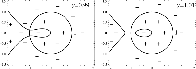
One of the key steps in the steepest-descent analysis of Riemann–Hilbert problems is the introduction of the so-called $g$ -function. For the Riemann–Hilbert problem 4.1 for discrete orthogonal polynomials, the $g$ -function is given by $g(z)=\int_{|s|=1}\log(z-s)\,d\mu(s)$ where $d\mu(s)$ is the so-called equilibrium measure satisfying $0\leq d\mu(s)\leq\frac{2m}{n}\frac{ds}{2\pi is}$ ; see, for example, BKMM . The upper-constraint $d\mu(s)\leq\frac{2m}{n}\frac{ds}{2\pi is}$ is due to the fact that the weight is discrete. The support of $d\mu$ consists of three types of intervals, voids (where $d\mu=0$ ), bands [where $0<d\mu(s)<\frac{2m}{n}\frac{ds}{2\pi is}$ ] and saturations [where $d\mu(s)=\frac{2m}{n}\frac{ds}{2\pi is}$ ].

For the continuous Riemann–Hilbert problem, the upper-constraint for the equilibrium is not present, and there are no saturations. For the Riemann–Hilbert Problem 4.2, it was shown in BDJ that with $\gamma=\frac{n}{2t}$ ,¹¹1This is actually the inverse of the parameter appearing in BDJ which we find more convenient to work with presently. the support of the equilibrium measure consists of the entire unit circle when $\gamma>1$ , and consists of single void and band intervals, with the void set centered about $z=-1$ , when $\gamma<1$ .

In the discrete Problem 4.1 the solution $\mathbf{Y}$ now depends on the three parameters $(t,n,m)$ and as we shall see in Section 5, the equilibrium measure’s support depends critically on the two parameters

\gamma=\frac{n}{2t}\quad\mbox{and}\quad\tilde{\gamma}=\frac{2m-n}{2t}.

(70)

As each of these parameters passes through the critical value $\gamma_{\mathrm{crit}}=1$ a transition occurs in the support of the equilibrium measure.

It turns out that to prove Theorems 1.1–1.3, we only need to evaluate $\mathbf{Y}(0;t,n,m)$ in two regimes: the “exponentially small regime”

n\geq 2t(1+\delta),\qquad 2m-n\geq 2t(1+\delta)

(71)

for a fixed $\delta>0$ , and the “Painlevé regime”

2t-Lt^{1/3}\leq n\leq 2t(1+\delta),\qquad 2t-Lt^{1/3}\leq 2m-n\leq 2t(1+\delta)

(72)

for fixed $L>0$ and $\delta>0$ . In the “exponential” case $\gamma,\tilde{\gamma}\geq 1+\delta$ and the equilibrium measure is supported on the whole of $\Sigma$ , while in the “Painlevé” case $\gamma,\tilde{\gamma}\in[1-\frac{L}{2}t^{-2/3},1+\delta]$ and the equilibrium measure is in the transitional region where a void and saturation region are beginning to open at $z=-1$ and $z=1$ , respectively. As such we never need to consider cases in which either a void or saturation have fully opened, and we restrict our attention to the full band (and the transitional) case only, focusing on obtaining the three lower-order terms of the asymptotic expansion explicitly. In this case the $g$ -function is explicit, and the transformations of the Riemann–Hilbert problem will be all stated explicitly without mentioning the $g$ -function in the subsequent sections.

There are many interesting related problems in which one needs an asymptotic description of the $\pi_{n,m}$ for a whole range of degrees $n$ ; one such example which we plan to study in the future is the Ablowtiz–Ladik equations. There we will fully describe the structure of the equilibrium measure in the full range of parameter space.

The analyses of the discrete and continuous Riemann–Hilbert problems have strong similarities, and we analyze them simultaneously. The important fact, which we clarify in Sections 6.2–6.3, is that in the discrete Riemann–Hilbert problem we can partition the solution into terms that come from (two) continuous Riemann–Hilbert problems which correspond to the marginal distributions and the remaining “joint” terms which contribute only to the joint distribution.

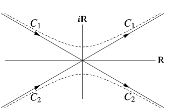
5 The exponentially small regime

The first steps of the steepest-descent analysis are the same for both the exponentially small regime and the Painlevé regime. We begin by first considering parameters $(n,m,t)$ in the “exponentially small regime” (71),

n\geq 2t(1+\delta),\qquad 2m-n\geq 2t(1+\delta)

for fixed $\delta>0$ . We assume that $\delta<1/2$ ; see the discussion before (90).

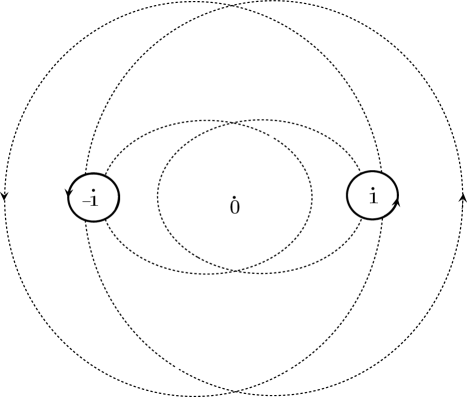
We begin our analysis of RHP 4.1 by first introducing a transformation $\mathbf{Y}\mapsto\mathbf{Q}$ such that the new unknown $\mathbf{Q}$ has no poles. Let $\Sigma$ denote the unit circle and let $\Sigma_{\mathrm{in}}$ and $\Sigma_{\mathrm{out}}$ denote positively oriented simple closed contours enclosing the origin such that $\Sigma_{\mathrm{in}}\subset\{z\dvtx|z|<1\}$ and $\Sigma_{\mathrm{out}}\subset\{z\dvtx|z|>1\}$ ; let $\Omega_{+}$ and $\Omega_{-}$ denote the nonempty open sets enclosed between $\Sigma$ and $\Sigma_{\mathrm{in}}$ and $\Sigma$ and $\Sigma_{\mathrm{out}}$ , respectively; see Figure 4. Define

\displaystyle\mathbf{Q}(z):=\cases{\mathbf{Y}(z)\pmatrix{1&\displaystyle\frac{z^{2m}}{z^{2m}-1}z^{-n}e^{t(z+z^{-1})}\vskip 2.0pt\cr 0&1},&\quad$z\in\Omega_{+}$,\cr\mathbf{Y}(z)\pmatrix{1&\displaystyle\frac{1}{z^{2m}-1}z^{-n}e^{t(z+z^{-1})}\vskip 2.0pt\cr 0&1},&\quad$z\in\Omega_{-}.$}

(73)

The triangular factors introduced in the above definition have poles at each $\omega_{r}$ , and the residues are such that the new unknown $\mathbf{Q}(z)$ has no poles, but is now piecewise holomorphic. Note that the residue of each triangular factor at each $z=\omega_{r}$ is the same since $z^{2m}=1$ at $z=\omega_{r}$ . Two different extensions of $\mathbf{Q}$ as above were introduced in KMM ; see also BKMM . By explicit computation $\mathbf{Q}(z)$ satisfies

Riemann–Hilbert Problem 5.1 (for Q(z)).

Find a $2\times 2$ matrix $\mathbf{Q}(z)$ such that: {longlist}[(1)]

$\mathbf{Q}(z)$ is analytic in $\mathbb{C}\setminus(\Sigma\cup\Sigma_{\mathrm{in}}\cup\Sigma_{\mathrm{out}})$ .

$\mathbf{Q}(z)=[I+\mathcal{O}(1/z)]z^{n\sigma_{3}}$ as $z\to\infty$ .

Along each jump contour $\mathbf{Q}_{+}(z)=\mathbf{Q}_{-}(z)V_{Q}(z)$ where

\displaystyle V_{Q}(z)=\cases{\pmatrix{1&\displaystyle z^{-n}e^{t(z+z^{-1})}\vskip 2.0pt\cr 0&1},&\quad$z\in\Sigma$,\vskip 3.0pt\cr\pmatrix{1&\displaystyle\frac{-z^{2m}}{z^{2m}-1}z^{-n}e^{t(z+z^{-1})}\vskip 2.0pt\cr 0&1},&\quad$z\in\Sigma_{\mathrm{in}}$,\vskip 3.0pt\cr\pmatrix{1&\displaystyle\frac{1}{z^{2m}-1}z^{-n}e^{t(z+z^{-1})}\vskip 2.0pt\cr 0&1},&\quad$z\in\Sigma_{\mathrm{out}}.$}

(74)

Once we transforms a RHP with poles to a “continuous” RHP as $\mathbf{Q}$ , the next step is to introduce a “ $g$ -function.” However, for the above RHP, when the parameters are in the regimes (71) and (72), it turns out that the $g$ -function is simple and explicit. We proceed by explicitly defining

\displaystyle\mathbf{S}(z):=\cases{\mathbf{Q}(z)\pmatrix{e^{tz}&0\vskip 2.0pt\cr 0&e^{-tz}}\pmatrix{0&-1\vskip 2.0pt\cr 1&0},&\quad$|z|<1$,\vskip 3.0pt\cr\mathbf{Q}(z)\pmatrix{z^{-n}e^{tz^{-1}}&0\vskip 2.0pt\cr 0&z^{n}e^{-tz^{-1}}},&\quad$|z|>1$.}

(75)

Clearly $\mathbf{Y}(0)=\mathbf{S}(0)({0\enskip 1\atop-1\enskip 0})$ and $\mathbf{S}(z)=I+\mathcal{O}(z^{-1})$ for large $z$ . Calculating the new jump matrices, we arrive at the following problem for $\mathbf{S}(z)$ .

Riemann–Hilbert Problem 5.2 (for $S(z)$ ).

Find a $2\times 2$ matrix-valued function $\mathbf{S}(z)$ such that: {longlist}[(1)]

$\mathbf{S}(z)$ is analytic for $z\in\mathbb{C}\setminus(\Sigma\cup\Sigma_{\mathrm{in}}\cup\Sigma_{\mathrm{out}})$ .

$\mathbf{S}(z)=I+\mathcal{O}(1/z)$ as $z\to\infty$ .

The boundary values of $\mathbf{S}(z)$ satisfy the jump relation $\mathbf{S}_{+}(z)=\break\mathbf{S}_{-}(z)V_{S}(z)$ where

\displaystyle V_{S}(z)=\cases{\displaystyle\pmatrix{1&0\vskip 2.0pt\cr(-1)^{n}e^{-2t\theta}&1}\pmatrix{1&\displaystyle-(-1)^{n}e^{2t\theta}\vskip 2.0pt\cr 0&1},&\quad$z\in\Sigma$,\vskip 3.0pt\cr\pmatrix{1&0\vskip 2.0pt\cr\displaystyle\frac{-1}{1-z^{2m}}e^{-2t\phi}&1},&\quad$z\in\Sigma_{\mathrm{in}}$,\vskip 3.0pt\cr\pmatrix{1&\displaystyle\frac{1}{1-z^{-2m}}e^{2t\phi}\vskip 2.0pt\cr 0&1},&\quad$z\in\Sigma_{\mathrm{out}}$,}

(76)

where

	$\displaystyle\theta(z;\gamma)$	$\displaystyle:=$	$\displaystyle\frac{1}{2}\bigl{(}z-z^{-1}\bigr{)}+\gamma\log(-z),\qquad\gamma:=\frac{n}{2t},$
	$\displaystyle\phi(z;\tilde{\gamma})$	$\displaystyle:=$	$\displaystyle\frac{1}{2}\bigl{(}z-z^{-1}\bigr{)}-\tilde{\gamma}\log z,\qquad\tilde{\gamma}:=\frac{2m-n}{2t}.$

Here the log is defined on the principal branch.

Now we assume that the parameters are in regime (71). Note that for any $e^{i\alpha}\in\Sigma$ , $\theta(e^{i\alpha})\in i\mathbb{R}$ . Also note that writing $z=re^{i\alpha}$ , we have $\frac{{d}}{{d}r}[\operatorname{Re}\theta(re^{i\alpha};\break\gamma)]_{r=1}=\cos\alpha+\gamma\geq-1+\gamma\geq\delta>0$ and $\frac{d^{2}}{dr^{2}}[\operatorname{Re}\theta(re^{i\alpha};\gamma)]_{r=1}=-r^{3}\cos\alpha-\gamma r^{-2}\leq r^{-3}-\gamma r^{-2}<0$ if $r>\gamma^{-1}$ . Hence $\operatorname{Re}\theta(re^{i\alpha};\gamma)\leq(-1+\gamma)(r-1)$ for $r\in(\gamma^{-1},1)$ and for all $\alpha\in(-\pi,\pi]$ . Therefore, for a given $\delta>0$ , there exist $0<r_{1}<r_{2}<1$ and $c>0$ such that $\operatorname{Re}[\frac{1}{\gamma}\theta(re^{i\alpha};\gamma)]\leq-c$ for all $r\in[r_{1},r_{2}]$ , $\alpha\in(-\pi,\pi]$ and for the parameters $(n,m,t)$ in the regime (71). Note that this implies that

\bigl{|}e^{2t\theta(z;\gamma)}\bigr{|}=e^{n\operatorname{Re}[(1/{\gamma)}\theta(re^{i\alpha};\gamma)]}\leq e^{-cn},\qquad r_{1}\leq|z|\leq r_{2}

(78)

for parameters $(n,m,t)$ in the regime (71).

Similarly, $\operatorname{Re}[\frac{1}{\tilde{\gamma}}\phi(\frac{1}{r}e^{i\alpha};\tilde{\gamma})]\leq-c$ for all $r\in[r_{1},r_{2}]$ , $\alpha\in(-\pi,\pi]$ and for the parameters $(n,m,t)$ in the regime (71). This can be easily seen by noting that $\phi(z;\gamma)=\theta(-z^{-1};\gamma)$ . Hence

\displaystyle\bigl{|}e^{2t\phi(z;\tilde{\gamma})}\bigr{|}=e^{(2m-n)\operatorname{Re}[(1/{\gamma})\theta(re^{i\alpha};\gamma)]}\leq e^{-c(2m-n)},\qquad\frac{1}{r_{1}}\leq|z|\leq\frac{1}{r_{2}}

(79)

for parameters $(n,m,t)$ in the regime (71).

Let $C_{\mathrm{in},-1},C_{\mathrm{in},1},C_{\mathrm{out},1}$ and $C_{\mathrm{out},-1}$ be the contours as depicted in Figure 5 such that $C_{\mathrm{in},-1}$ and $C_{\mathrm{in},1}$ lie in the annulus $r_{1}<|z|<r_{2}$ and $C_{\mathrm{out},1}$ and $C_{\mathrm{out},-1}$ lie in the annulus $\frac{1}{r_{1}}<|z|<\frac{1}{r_{2}}$ . Make now the following change of variables which moves the oscillations on $\Sigma$ into regions of exponential decay.

\displaystyle\mathbf{T}(z)=\cases{\displaystyle\mathbf{S}(z)\pmatrix{1&(-1)^{n}e^{2t\theta}\vskip 2.0pt\cr 0&1},&\quad$z\in\Omega_{+,0}$,\vskip 3.0pt\cr\mathbf{S}(z)\pmatrix{1&(-1)^{n}e^{2t\theta}\vskip 2.0pt\cr 0&1}\pmatrix{1&0\vskip 2.0pt\cr-e^{-2t\phi}&1},&\quad$z\in\Omega_{+,1}$,\vskip 3.0pt\cr\mathbf{S}(z)\pmatrix{1&0\vskip 2.0pt\cr(-1)^{n}e^{-2t\theta}&1},&\quad$z\in\Omega_{-,0}$,\vskip 3.0pt\cr\mathbf{S}(z)\pmatrix{1&0\vskip 2.0pt\cr(-1)^{n}e^{-2t\theta}&1}\pmatrix{1&-e^{2t\phi}\vskip 2.0pt\cr 0&1},&\quad$z\in\Omega_{-,1}$,\cr\mathbf{S}(z),&\quad$\mbox{elsewhere.}$}

(80)

Note that $\mathbf{Y}(0)=\mathbf{T}(0)({0\enskip 1\atop-1\enskip 0})$ . Explicitly calculating the new jumps, the new unknown $\mathbf{T}(z)$ satisfies the following problem:

Riemann–Hilbert Problem 5.3 (for T(z)).

Find a $2\times 2$ matrix-valued function $\mathbf{T}(z)$ satisfying the following properties:

[(1)]
(1)

$\mathbf{T}(z)$ is analytic in $\mathbb{C}\setminus(\Sigma_{\mathrm{in}}\cup\Sigma_{\mathrm{out}}\cup C_{\mathrm{in},\pm 1}\cup C_{\mathrm{out},\pm 1})$ .
(2)

$\mathbf{T}(z)=I+\mathcal{O}(1/z)$ as $z\to\infty$ .

(3)

The boundary values of $\mathbf{T}(z)$ satisfy the jump relation $\mathbf{T}_{+}(z)=\break\mathbf{T}_{-}(z)V_{T}(z)$ where

\displaystyle V_{T}(z)

\displaystyle=

\displaystyle\cases{\displaystyle\pmatrix{1&-(-1)^{n}e^{2t\theta}\vskip 2.0pt\cr 0&1},&\quad$z\in C_{\mathrm{in},-1}$,\vskip 3.0pt\cr\displaystyle\pmatrix{1&0\vskip 2.0pt\cr(-1)^{n}e^{-2t\theta}&1},&\quad$z\in C_{\mathrm{out},-1}$,\vskip 3.0pt\cr\pmatrix{1&0\vskip 2.0pt\cr\displaystyle-e^{-2t\phi}&1},&\quad$z\in C_{\mathrm{in},1}$,\vskip 3.0pt\cr\pmatrix{1&\displaystyle e^{2t\phi}\vskip 2.0pt\cr 0&1},&\quad$z\in C_{\mathrm{out},1}$,\vskip 3.0pt\cr\pmatrix{1&0\vskip 2.0pt\cr\displaystyle\frac{-e^{-2t\phi}}{1-z^{2m}}&1},&\quad$z\in\Sigma_{\mathrm{in},-1}$,\vskip 3.0pt\cr\pmatrix{1&\displaystyle\frac{-(-1)^{n}e^{-2t\theta}}{1-z^{2m}}\vskip 2.0pt\cr 0&1}\bigl{(}1-z^{2m}\bigr{)}^{-\sigma_{3}},&\quad$z\in\Sigma_{\mathrm{in},1}$,\vskip 3.0pt\cr\displaystyle\bigl{(}1-z^{-2m}\bigr{)}^{-\sigma_{3}}\pmatrix{1&0\vskip 2.0pt\cr\displaystyle\frac{(-1)^{n}e^{-2t\theta}}{1-z^{-2m}}&1},&\quad$z\in\Sigma_{\mathrm{out},1}$,\vskip 3.0pt\cr\pmatrix{1&\displaystyle\frac{1}{1-z^{-2m}}e^{2t\phi}\vskip 2.0pt\cr 0&1},&\quad$z\in\Sigma_{\mathrm{out},-1}.$}

(81)

Then from (78) and (79), we find that $V_{T}(z)=I+\mathcal{O}(e^{-c\max\{n,2m-n\}})$ uniformly for $z$ on the contour. Hence we obtain the following result.

Proposition 5.1.

Let $\mathbf{Y}(z;t,n,m)$ be the solution to the RHP (4.1). For any $\delta>0$ , there exists a constant $c>0$ such that, if

n\geq 2t(1+\delta),\qquad 2m-n\geq 2t(1+\delta),

(82)

then

\mathbf{Y}(0;t,n,m)\pmatrix{0&-1\cr 1&0}=I+\mathcal{O}\bigl{(}e^{-c\max\{n,2m-n\}}\bigr{)}.

(83)

In particular,

\pi_{n,m}(0;t)=\mathcal{O}\bigl{(}e^{-c\max\{n,2m-n\}}\bigr{)}.

(84)

6 Painlevé regime

We now consider the parameters $(n,m,t)$ in regime (72),

2t-Lt^{1/3}\leq n\leq 2t(1+\delta),\qquad 2t-Lt^{1/3}\leq 2m-n\leq 2t(1+\delta)

(85)

for fixed $L>0$ and $\delta>0$ . We assume that $\delta<1/2$ ; see the discussion before (90).

Let $\mathbf{S}(z)$ be same as in the previous section. When $\gamma\in[1-\delta,1+\delta]$ , estimate (78) does not hold any more. However, it is easy to check using a similar calculation as before that the exponential decay still holds in an annular sector away from the point $z=-1$ . [Note that the (double) critical point of $\theta(z;1)$ is $z=-1$ .] More precisely, one can check that given $\delta\in(0,1)$ , there exist positive constants $\alpha_{1}\geq O(\delta^{1/2})>0$ and $\rho_{1}\geq O(\delta^{1/2})$ such that if $\gamma\in[1-\delta,1+\delta]$ , then $|e^{2\theta(z;\gamma)}|<1$ for $z$ in the annular sector $\mathcal{S}_{\mathrm{in},-1}:=\{z=re^{i\alpha}\dvtx\rho_{1}<r<1,|\alpha|<\pi-\alpha_{1}\}$ . Moreover, if $z$ is in a compact subset of $\mathcal{S}_{\mathrm{in},-1}$ , then there exists $c>0$ such that $|e^{2\theta(z;\gamma)}|\leq e^{-c}$ uniformly in $\gamma\in[1-\delta,1+\delta]$ ; see Figure 6.

Similarly, from the symmetry $\phi(z;\gamma)=\theta(-z^{-1};\gamma)$ , under the same assumptions, $|e^{2\phi(z;\tilde{\gamma})}|<1$ for $z$ in the annular sector $\mathcal{S}_{\mathrm{out},1}:=\{z=\frac{1}{r}e^{i\alpha}\dvtx\rho_{1}<r<1,\alpha_{1}\leq|\alpha|\leq\pi\}$ . Note the change of the condition on the angle from $\mathcal{S}_{\mathrm{in},-1}$ ; the (double) critical point of $\phi(z;1)$ is $z=1$ . As before, if $z$ is in a compact subset of $\mathcal{S}_{\mathrm{out},1}$ , then there exists $c>0$ such that $|e^{2\phi(z;\gamma)}|\leq e^{-c}$ uniformly in $\gamma\in[1-\delta,1+\delta]$ .

Now define $\mathbf{T}$ by (80) as before. In doing so, we take $C_{\mathrm{in},1}$ and $C_{\mathrm{in},-1}$ to lie in the annulus $\rho_{1}<|z|<1$ , and take $C_{\mathrm{out},1}$ and $C_{\mathrm{out},-1}$ to lie in the annulus $1<|z|<1/\rho_{1}$ . Then the jump matrix in (81) satisfies

V_{T}(z)=I+\mathcal{O}\bigl{(}e^{-ct}\bigr{)}

(86)

uniformly for $\gamma,\tilde{\gamma}\in[1-\delta,1+\delta]$ and for $z$ in all the contours except for $(C_{\mathrm{in},-1}\cup C_{\mathrm{out},-1})\cap\{|\operatorname{arg}(z)|>\pi-\alpha_{1}\}$ and $(C_{\mathrm{in},1}\cup C_{\mathrm{out},1})\cap\{|\operatorname{arg}(z)|<\alpha_{1}\}$ . The parts of the contour where (86) is not valid are handled by introducing local parametrix that can be solved by the RHP for the Painlevé II equation; see Section 10. Such a “Painlevé parametrix” was introduced in the analysis of BDJ on a similar orthogonal polynomials but with a continuous weight. A drawback of the analysis of BDJ was that the parametrix was solved asymptotically rather than exactly as in other cases such as DKMVZa , DKMVZb . The exactly matching Painlevé parametrix was constructed later in CK . The construction of CK requires, in the context of this paper, that $\gamma\in[1-Lt^{-2/3},1+Lt^{-2/3}]$ . In a recent paper BMiller , a different approach to the exact construction of the Painlevé parametrix was introduced. This construction has the advantage that it works for all $\gamma$ (and $\tilde{\gamma}$ ) in regime (72).

We seek a global parametrix in the form

\mathbf{A}(z)=\cases{\mathbf{A}_{1}(z),&\quad$z\in\mathcal{U}_{1}$,\cr\mathbf{A}_{-1}(z),&\quad$z\in\mathcal{U}_{-1}$,\cr I,&\quad$\mbox{elsewhere},$}

(87)

where $\mathcal{U}_{\pm 1}$ are sufficiently small, fixed size, neighborhoods of $\pm 1$ . Later we will fix the size of $\mathcal{U}_{\pm 1}$ first and then choose $\delta$ small enough so that $\mathcal{U}_{-1}$ contains $(C_{\mathrm{in},-1}\cup C_{\mathrm{out},-1})\cap\{|\operatorname{arg}(z)|>\pi-\alpha_{1}\}$ and $\mathcal{U}_{1}$ contains $(C_{\mathrm{in},1}\cup C_{\mathrm{out},1})\cap\{|\operatorname{arg}(z)|<\alpha_{1}\}$ so that (86) is valid for all $z$ in the contour of $\mathbf{T}$ except for in $\mathcal{U}_{\pm 1}$ .

6.1 Local models near $1$ and $-1$

In order to construct exactly matching parametrices $\mathbf{A}_{\pm 1}$ , we need to introduce Langer transformations which map the local phase functions $\theta$ and $\phi$ to the Painlevé phase (213) in $\mathcal{U}_{-1}$ and $\mathcal{U}_{1}$ , respectively.

The phase $\theta(z;\gamma)$ is analytic in $z$ in the neighborhood $|z+1|<1$ (and entire in $\gamma$ ) and admits the expansion

	$\displaystyle\theta(z;\gamma)$	$\displaystyle=$	$\displaystyle(1-\gamma)(z+1)+\frac{1-\gamma}{2}(z+1)^{2}+\frac{3-2\gamma}{6}(z+1)^{3}$
			$\displaystyle{}+\mathcal{O}\bigl{(}(z+1)^{4}\bigr{)}.$

At the critical value $\gamma=1$ the expansion degenerates to a cubic at leading order; for values of $\gamma$ near $1$ the cubic unfolds either into three real or one real and two complex roots near $z=-1$ . The double critical point–double root of $\theta^{\prime}(z;1)$ –unfolds into a pair of simple critical points near $z=-1$ ,

\displaystyle\frac{{d}\theta}{{d}z}=0\quad\Rightarrow\quad z_{\pm}=-\gamma\pm\sqrt{\gamma^{2}-1}.

(89)

Note that the relation $\phi(z;\tilde{\gamma})=-\theta(-z;\tilde{\gamma})$ implies that $\phi$ admits a similar expansion about $z=1$ with the same structure.

As the cubic coefficient in (6.1) is bounded away from zero (note that $\gamma\leq 1+\delta<3/2$ ) we make use of a classical result of CFU to introduce new parameters $a(\gamma)$ and $b(\gamma)$ such that the relation

\tfrac{4}{3}f(z;\gamma)^{3}+a(\gamma)f(z;\gamma)+b(\gamma)=-i\theta(z;\gamma),\qquad z\in\mathcal{U}_{-1}

(90)

defines an invertible conformal mapping $f=f(z)$ from a sufficiently small, $\gamma$ -independent, neighborhood $\mathcal{U}_{-1}$ onto $f(\mathcal{U}_{1})$ such that the parameters $a$ and $b$ depend continuously on $\gamma$ near $1$ . It was shown in CFU (see also Friedman ) that there exist $\delta_{1}>0$ and a $\gamma$ -independent neighborhood $\mathcal{U}_{-1}$ such that the above map is conformal in $\mathcal{U}_{-1}$ for all $\gamma\in[1-\delta_{1},1+\delta_{1}]$ if the critical points $f_{\pm}=\pm\sqrt{-a}/2$ of the left-hand side, seen as a function of $f$ , correspond to the critical points $z_{\pm}$ of $\theta(z;\gamma)$ . This means that the left-hand side of (90) evaluated at $f=f_{\pm}$ should equal to the right-hand side of (90) evaluated at $z=z_{\pm}$ . These two conditions determine parameters $a$ and $b$ as

	$\displaystyle b(\gamma)$	$\displaystyle=$	$\displaystyle\frac{-i}{2}\bigl{[}\theta(z_{+};\gamma)+\theta(z_{-};\gamma)\bigr{]},$
	$\displaystyle\bigl{(}-a(\gamma)\bigr{)}^{3/2}$	$\displaystyle=$	$\displaystyle\frac{3i}{2}\bigl{(}\theta(z_{+};\gamma)-\theta(z_{-};\gamma)\bigr{)}.$

Since $\theta(z_{+};\gamma)=-\theta(z_{-};\gamma)=\sqrt{\gamma^{2}-1}-\gamma\log(\gamma+\sqrt{\gamma^{2}-1})$ , we have

b(\gamma)=0.

(92)

There are three choices of branch of $a(\gamma)$ . We choose the branch so that

a(\gamma)=-\bigl{[}3i\bigl{(}\sqrt{\gamma^{2}-1}-\gamma\log\bigl{(}\gamma+\sqrt{\gamma^{2}-1}\bigr{)}\bigr{)}\bigr{]}^{2/3}

(93)

satisfies the power series expansion

a(\gamma)=2(\gamma-1)-\tfrac 1{15}(\gamma-1)^{2}+\mathcal{O}\bigl{(}(\gamma-1)^{3}\bigr{)}.

(94)

To verify this, it is useful to note that $\frac{d^{2}}{d\gamma^{2}}[\sqrt{\gamma^{2}-1}-\gamma\log(\gamma+\sqrt{\gamma^{2}-1})]=-(\gamma^{2}-1)^{-1/2}$ . With this choice of $a$ , we have

	$\displaystyle f(z;\gamma)$	$\displaystyle=$	$\displaystyle\frac{i(\gamma-1)}{a}(z+1)+\frac{i(\gamma-1)}{2a}(z+1)^{2}$
			$\displaystyle{}+\frac{1}{6i}\biggl{(}\frac{3-2\gamma}{a}-8\frac{(\gamma-1)^{3}}{a^{4}}\biggr{)}(z+1)^{3}+\mathcal{O}\bigl{(}(z+1)^{4}\bigr{)}.$

Inserting (94), we obtain

$\displaystyle f(z;\gamma)$	$\displaystyle=$	$\displaystyle\frac{i}{2}(z+1)\biggl{[}1+\frac{1}{2}(z+1)+\frac{7}{20}(z+1)^{2}+\mathcal{O}\bigl{(}(z+1)^{3}\bigr{)}\biggr{]}$
		$\displaystyle{}+\frac{i}{60}(\gamma-1)(z+1)\biggl{[}1+\frac{1}{2}(z+1)+\mathcal{O}\bigl{(}(z+1)^{2}\bigr{)}\biggr{]}$
		$\displaystyle{}+\mathcal{O}\bigl{(}(\gamma-1)^{2}(z+1)\bigr{)}.$

Define the rescaled coordinates (Langer coordinates) $\zeta=\zeta(z;\gamma)=\break t^{1/3}f(z;\gamma)$ for $z\in\mathcal{U}_{-1}$ , and set

s=s(\gamma)=t^{2/3}a(\gamma).

(97)

Then [see (213)]

\displaystyle t\theta(z;\gamma)=i\bigl{(}\tfrac{4}{3}\zeta^{3}+s\zeta\bigr{)}=i\theta_{\mathit{PII}}(\zeta,s),\qquad z\in\mathcal{U}_{-1}.

(98)

We note from (94) that for the parameters $(n,m,t)$ in regime (72),

s(\gamma)\geq-2L

(99)

for all large enough $t$ . We also have

s(\gamma)=2t^{2/3}(\gamma-1)-\frac{(2t^{2/3}(\gamma-1))^{2}}{60}t^{-2/3}+\mathcal{O}\bigl{(}t^{2/3}(\gamma-1)^{3}\bigr{)}.

(100)

We introduce similar coordinates in $\mathcal{U}_{1}$ . This can be easily achieved by noting the symmetry $\phi(z,\tilde{\gamma})=-\theta(-z,\tilde{\gamma})$ . We set $\mathcal{U}_{1}=-\mathcal{U}_{-1}$ and define $f(z;\tilde{\gamma}):=-f(-z;\tilde{\gamma})$ for $z\in\mathcal{U}_{1}$ . Then we find, with the same choice of $a$ and $b$ ,

\tfrac{4}{3}f(z;\tilde{\gamma})^{3}+a(\tilde{\gamma})f(z;\tilde{\gamma})=-i\phi(z;\tilde{\gamma}),\qquad z\in\mathcal{U}_{1}.

(101)

Defining $\zeta=\zeta(z;\gamma)=t^{1/3}f(z;\gamma)$ , $z\in\mathcal{U}_{-1}$ and $s=s(\gamma)=t^{2/3}a(\gamma)$ as before, we obtain

t\phi(z;\tilde{\gamma})=i\bigl{(}\tfrac{4}{3}\zeta(z;\tilde{\gamma})^{3}+s(\tilde{\gamma})\zeta(z;\tilde{\gamma})\bigr{)}=i\theta_{\mathit{PII}}(\zeta,s),\qquad z\in\mathcal{U}_{-1}.

(102)

Note the symmetry

\zeta(z;\tilde{\gamma})=-\zeta(-z;\tilde{\gamma}),\qquad z\in\mathcal{U}_{1}.

(103)

We take $\delta$ such that $\delta<\min\{1/2,\delta_{1}\}$ where $\delta_{1}$ we introduced in defining $f$ in (90). Then consider the parameters $(n,m,t)$ satisfying (72).

Consider the image of $\mathcal{U}_{-1}$ under the map $z\mapsto\zeta(z;\gamma)$ . From (6.1), we find that there exists $\delta_{2}>0$ such that for $\gamma\in[1-\delta_{2},1+\delta_{2}]$ , $\zeta(\mathcal{U}_{-1};\gamma)$ contains a disk centered at $0$ and of radius $\geq\mathcal{O}(t^{1/3})$ in the $\zeta$ -plane. The same holds for $\zeta(\mathcal{U}_{1};\tilde{\gamma})$ . Note that from (6.1), the image contours $\zeta(C_{-1,\mathrm{in}/\mathrm{out}})$ are oriented left-to-right and the image contours $\zeta(C_{1,\mathrm{in}/\mathrm{out}})$ are oriented right-to-left as depicted in Figure 7.

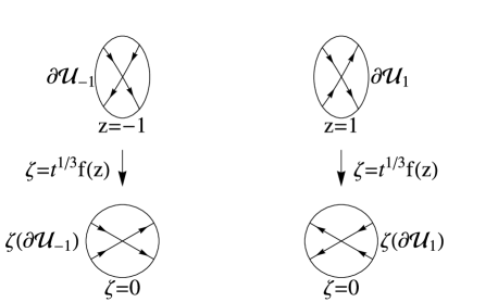
We now use $\zeta$ to map the local contours and jump matrices inside $\mathcal{U}_{\pm 1}$ onto the jumps of the Painlevé parametrix, RHP 10.1. We locally deform, if necessary, the contours $C_{\pm 1,\mathrm{in}/\mathrm{out}}$ so that the image contours $\zeta(C_{\pm 1,\mathrm{in}/\mathrm{out}}\cap\mathcal{U}_{\pm 1})$ become the rays $\Gamma_{i}$ , $i=1,3,4,6$ described in (206), and we extend $C_{\pm 1,\mathrm{in}/\mathrm{out}}\cap(\mathcal{U}_{-1}\cup\mathcal{U}_{1})$ to the rest of $C_{\pm 1,\mathrm{in}/\mathrm{out}}$ so that estimate (86) holds for $z$ on the contour outside of $\mathcal{U}_{\pm 1}$ . The exact shape of the contours are not important. Reorienting the image contours, if necessary, to go from left-to-right and using (98) and (102) the image contours and jumps are, up to a conjugation by a constant matrix, exactly those of the Painlevé parametrix, RHP 10.1.

Let $\bolds{\Psi}(\zeta,s)$ be the solution of the Painlevé II model problem, RHP 10.1. Set $\sigma_{2}=\bigl{(}{0\enskip-i\atop i\enskip 0}\bigr{)}$ and recall that $\sigma_{3}=\bigl{(}{1\enskip 0\atop 0\enskip 1}\bigr{)}$ . Taking into account the orientation of $\zeta(C_{\pm 1,\mathrm{in}/\mathrm{out}}\cap\mathcal{U}_{\pm 1})$ , we define the local models

	$\displaystyle\mathbf{A}_{-1}(z)$	$\displaystyle=$	$\displaystyle\mathbf{A}_{-1}(z;\gamma):=\sigma_{2}\sigma_{3}^{n}\bolds{\Psi}\bigl{(}\zeta(z;\gamma);s(\gamma)\bigr{)}\sigma_{3}^{n}\sigma_{2},\qquad z\in\mathcal{U}_{-1},$
	$\displaystyle\mathbf{A}_{1}(z)$	$\displaystyle=$	$\displaystyle\mathbf{A}_{1}(z;\tilde{\gamma}):=\sigma_{2}\bolds{\Psi}\bigl{(}\zeta(z;\tilde{\gamma});s(\tilde{\gamma})\bigr{)}\sigma_{2},\qquad z\in\mathcal{U}_{1}.$

Note from symmetries (214) and (103) that these two models are related as

\mathbf{A}_{1}(z,\tilde{\gamma})=\sigma_{1}\sigma_{3}^{n}\mathbf{A}_{-1}(-z,\tilde{\gamma})\sigma_{3}^{n}\sigma_{1},\qquad z\in\mathcal{U}_{1}.

(105)

From (98) and (102), $\mathbf{A}_{\pm 1}(z)$ satisfies the same jump condition as $\mathbf{T}(z)$ in $\mathcal{U}_{\pm 1}$ , respectively.

Define the ratio of the global parametrix to the exact problem $\mathbf{T}(z)$ ,

\mathbf{R}(z)=\mathbf{T}(z)\mathbf{A}^{-1}(z).

(106)

Then $\mathbf{R}(z)$ has no jumps inside $\mathcal{U}_{\pm 1}$ , but gains jumps on the positively oriented boundaries $\partial\mathcal{U}_{\pm 1}$ . Let $\Sigma_{R}^{0}=\Sigma_{\mathrm{in}}\cup\Sigma_{\mathrm{out}}\cup C_{\mathrm{in},\pm 1}\cup C_{\mathrm{out},\pm 1}\setminus(\mathcal{U}_{1}\cup\mathcal{U}_{-1})$ ; see Figure 8. Then $\mathbf{R}$ satisfies the following problem:

Riemann–Hilbert Problem 6.1 (for $\mathbf{R}(z)$ ).

Find a $2\times 2$ matrix $\mathbf{R}(z)$ such that: {longlist}[(1)]

$\mathbf{R}(z)$ is analytic in $\mathbb{C}\setminus\Sigma_{R}$ where $\Sigma_{R}=\Sigma_{R}^{0}\cup\partial\mathcal{U}_{1}\cup\partial\mathcal{U}_{-1}$ .

$\mathbf{R}(z)\to I$ as $z\to\infty$ .

The boundary values of $\mathbf{R}$ satisfy the jump relation $\mathbf{R}_{+}=\mathbf{R}_{-}V_{R}$ where

\displaystyle V_{R}(z)=\cases{\mathbf{A}_{1}(z)^{-1},&\quad$z\in\partial\mathcal{U}_{1}$,\cr\mathbf{A}_{-1}(z)^{-1},&\quad$z\in\partial\mathcal{U}_{-1}$,\cr V_{T}(z),&\quad$z\in\Sigma_{R}^{0}$.}

(107)

The jumps of $\mathbf{R}(z)$ are now everywhere uniformly near identity. In fact, for the parameters $(n,m,t)$ in regime (72), it follows from (86),

\|V_{R}-I\|_{L^{\infty}(\Sigma_{R}^{0})}=\mathcal{O}\bigl{(}e^{-ct}\bigr{)},

(108)

and from (6.1) and (216) that (recall that $\zeta(\mathcal{U}_{\pm 1};\gamma)$ contains a disk of radius $\geq\mathcal{O}(t^{1/3})$ for all $\gamma\in[1-\delta,1+\delta]$ )

\|V_{R}-I\|_{L^{\infty}(\mathcal{U}_{\pm 1})}=\mathcal{O}\bigl{(}t^{-1/3}\bigr{)}.

(109)

(We will use a better estimate for the latter below.) The above estimates establish that $\mathbf{R}$ falls into the class of small norm RHPs for any sufficiently large $t$ . Let $C_{-}\dvtx L^{2}(\Sigma_{R})\to L^{2}(\Sigma_{R})$ denote the usual Cauchy projection operator and define

\displaystyle\qquad C_{V_{R}}[f](z):=C_{-}\bigl{[}f(w)(V_{R}-I)\bigr{]}=\frac{1}{2\pi i}\int_{\Sigma_{R}}\frac{f(w)(V_{R}(w)-I)}{(w-z)_{-}}\,dw

(110)

and

\mathcal{K}_{R}[f](z):=\frac{1}{2\pi i}\int_{\Sigma_{R}}\frac{f(w)(V_{R}(w)-I)}{(w-z)}\,dw,

(111)

which maps $f\in L^{2}(\Sigma_{R})$ to an analytic function in $\mathbb{C}\setminus\Sigma_{R}$ . Then as $C_{-}$ is a bounded $L^{2}$ operator whose operator norm is uniformly bounded (see, e.g., BK ) and the contours $\Sigma_{R}$ are finite length, it follows that $\|C_{V_{R}}\|_{L^{2}\to L^{2}}=\mathcal{O}(t^{-1/3})$ for large $t$ which guarantees the existence of a unique solution to $(1-C_{V_{R}})\mu=I$ . Once the existence of $\mu(z)$ is established, it follows immediately from the general theory of RHPs that

\displaystyle\mathbf{R}(z):=I+\mathcal{K}_{R}[\mu](z)=I+\frac{1}{2\pi i}\int_{\Sigma_{R}}\frac{\mu(w)(V_{R}(w)-I)}{w-z}\,dw

(112)

is the solution of RHP 6.1.

Unfolding the series of transformations $\mathbf{Y}\mapsto\mathbf{Q}\mapsto\mathbf{S}\mapsto\mathbf{T}\mapsto\mathbf{R}$ we have $\mathbf{Y}(0)=\mathbf{R}(0)\bigl{(}{0\atop-1}\enskip{1\atop 0}\bigr{)}$ , and from (67) it follows that

\pi_{n,m}(0;t)=-\mathbf{R}_{12}(0;t,n,m)=\mathbf{R}_{21}(0;t,n,m).

(113)

We now evaluate $\mathbf{R}(0;t,n,m)$ explicitly for the first three terms in the asymptotic expansion. But we first consider the corresponding RHP for the continuous weight in the next subsection. We will compare the discrete weight problem to the continuous weight problem.

6.2 Analysis of the continuous weight problem

A streamlined version of the above procedure reducing the discrete problem, RHP 4.1, to small-norm form can be used to study the continuous weight problem, RHP 4.2. Using the same $g$ -function used in the discrete case, we define $\mathbf{Y}^{\infty}\mapsto\mathbf{S}^{\infty}$ as in (75), replacing $\mathbf{Q}$ with $\mathbf{Y}^{\infty}$ . The new RHP for $\mathbf{S}^{\infty}$ features the single phase $\theta(z;\gamma)$ defined by (5.2) which we recall has a critical value at $z=-1$ . In the “exponentially small regime” (71) estimate (78) holds and just as in Proposition 5.1, we have in the end

\pi_{n,\infty}(0;t)=\mathcal{O}\bigl{(}e^{-cn}\bigr{)}\qquad\mbox{for $(n,t)$ satisfying (\ref{eqregime1}).}

(114)

In the Painlevé regime (72), by introducing a simplified version of transformation (80), using only the factors appearing in $\Omega_{\pm,0}$ to open lenses, one defines a transformation $\mathbf{S}^{\infty}\mapsto\mathbf{T}^{\infty}$ . The problem for $\mathbf{T}^{\infty}$ is then approximated by a parametrix which is identity outside a neighborhood $\mathcal{U}_{-1}$ of $z=-1$ and inside $\mathcal{U}_{-1}$ is approximated by the same model as the discrete case, $\mathbf{A}_{-1}(z)$ defined by (6.1). The result is a small norm problem $\mathbf{R}^{\infty}$ for the continuous case where

\mathbf{R}^{\infty}(z)=I+\frac{1}{2\pi i}\int_{\Sigma_{R^{\infty}}}\frac{\mu^{\infty}(w)(V_{R^{\infty}}(w)-I)}{w-z}\,dw,

(115)

where

V_{R^{\infty}}(z)=\cases{\mathbf{A}_{-1}(z)^{-1},&\quad$z\in\partial\mathcal{U}_{-1}$,\cr I+\mathcal{O}\bigl{(}e^{-ct}\bigr{)},&\quad$z\in\Sigma_{R}^{\infty}\setminus\partial\mathcal{U}_{-1}$.}

(116)

Moreover, the continuous weight orthogonal polynomial $\pi_{n}^{\infty}(0)$ is given by

\qquad\pi_{n,\infty}(0;t)=-\mathbf{R}^{\infty}_{12}(0;t,n)=\mathbf{R}^{\infty}_{21}(0;t,n)\qquad\mbox{for $(n,t)$ satisfying (\ref{eqregime2}).}

(117)

6.3 Expansion of $\mathbf{R}(0)$

In this section we calculate the asymptotic expansion of

\displaystyle\mathbf{R}(0)=I+\mathcal{K}_{R}[\mu](0)=I+\frac{1}{2\pi i}\int_{\Sigma_{R}}\frac{\mu(w)(V_{R}(w)-I)}{w}\,dw

(118)

up to order $\mathcal{O}(t^{-1})$ . We begin by representing $\mu$ using its Nuemann series expansion,

\mu(z)=I+\sum_{k=1}^{\infty}(C_{R})^{k}[I],

(119)

which, due to (108) and (109), convergences uniformly and absolutely. In both (118) and (119), the dominant contribution to the integral comes from the boundaries $\partial\mathcal{U}_{\pm 1}$ . In fact, denoting by $P_{0}$ the projection operator onto $\Sigma_{R}\setminus(\partial\mathcal{U}_{-1}\cup\partial U_{1})$ , we find from (108) that $\|C_{R}P_{0}\|_{L^{2}(\Sigma_{R})\to L^{2}(\Sigma_{R})}=\mathcal{O}(e^{-ct})$ and $\|\mathcal{K}_{R}P_{0}\|_{L^{2}(\Sigma_{R})\to L^{2}(\Sigma_{R})}=\mathcal{O}(e^{-ct})$ .

Denoting by $P_{\pm 1}$ the projection operator onto $\partial\mathcal{U}_{\pm}$ , respectively, define $C_{\pm 1}:=C_{R}P_{\pm 1}$ and $\mathcal{K}_{\pm 1}:=\mathcal{K}_{R}P_{\pm 1}$ : for any $f\in L^{2}(\Sigma_{R})$ ,

	$\displaystyle C_{\pm 1}[f](z)$	$\displaystyle=$	$\displaystyle\frac{1}{2\pi i}\oint_{\partial\mathcal{U}_{\pm 1}}\frac{f(w)(V_{R}(w)-I)}{(w-z)_{-}}\,dw,\qquad z\in\Sigma_{R},$
	$\displaystyle\mathcal{K}_{\pm 1}[f](z)$	$\displaystyle=$	$\displaystyle\frac{1}{2\pi i}\oint_{\partial\mathcal{U}_{\pm 1}}\frac{f(w)(V_{R}(w)-I)}{(w-z)}\,dw,\qquad z\notin\Sigma_{R}.$

Then we find

\mathbf{R}(0)=I+(\mathcal{K}_{-1}+\mathcal{K}_{1})[\mu](0)+\mathcal{O}\bigl{(}e^{-ct}\bigr{)},

(121)

where

\mu(z)=I+\sum_{k=1}^{\infty}(C_{-1}+C_{1})^{k}[I](z)+\mathcal{O}\bigl{(}e^{-ct}\bigr{)}.

(122)

Recall $s(\gamma)$ defined in (97). Introduce the shorthand $s=s(\gamma)$ and $\tilde{s}=s(\tilde{\gamma})$ . Using (216), (217) and (6.1) we have


			$\displaystyle V_{R}(z)-I$
			$\displaystyle\qquad=\cases{\displaystyle\frac{\varphi_{1}(s)}{t^{1/3}f(z;\gamma)}+\frac{\varphi_{2}(s)}{t^{2/3}f(z;\gamma)^{2}}+\frac{\varphi_{3}(s)}{t^{-1}f(z;\gamma)^{3}}+\mathcal{O}\biggl{(}\frac{e^{-c_{0}\|s\|^{3/2}}}{t^{4/3}}\biggr{)},\vskip 3.0pt\cr\quad z\in\partial\mathcal{U}_{-1},\vskip 3.0pt\cr\displaystyle\frac{\phi_{1}(\tilde{s})}{t^{1/3}f(z;\tilde{\gamma})}+\frac{\phi_{2}(\tilde{s})}{t^{2/3}f(z;\tilde{\gamma})^{2}}+\frac{\phi_{3}(\tilde{s})}{t^{-1}f(z;\tilde{\gamma})^{3}}+\mathcal{O}\biggl{(}\frac{e^{-c_{0}\|s\|^{3/2}}}{t^{4/3}}\biggr{)},\vskip 3.0pt\cr\quad z\in\partial\mathcal{U}_{1},}$
with

	$\displaystyle\varphi_{1}(s)$	$\displaystyle=$	$\displaystyle\frac{1}{2i}\left[\matrix{-u(s)&-(-1)^{n}q(s)\cr(-1)^{n}q(s)&u(s)}\right],$
	$\displaystyle\qquad\quad\varphi_{2}(s)$	$\displaystyle=$	$\displaystyle\frac{1}{(2i)^{2}}\left[\matrix{\displaystyle\frac{1}{2}u(s)^{2}-\frac{1}{2}q(s)^{2}&(-1)^{n}\bigl{(}q(s)u(s)-q^{\prime}(s)\bigr{)}\cr(-1)^{n}\bigl{(}q(s)u(s)-q^{\prime}(s)\bigr{)}&\displaystyle\frac{1}{2}u(s)^{2}-\frac{1}{2}q(s)^{2}}\right],$	(123b)
	$\displaystyle\varphi_{3}(s)$	$\displaystyle=$	$\displaystyle\frac{1}{(2i)^{3}}\left[\matrix{\alpha(s)&(-1)^{n}\beta(s)\cr-(-1)^{n}\beta(s)&-\alpha(s)}\right]$
and
	$\phi_{k}(\tilde{s})=\sigma_{3}^{n}\varphi_{k}(\tilde{s})\sigma_{3}^{n},\qquad k=1,2,3,$			(123c)

where $q$ is defined by (10) and $u$ , $\alpha$ and $\beta$ are defined in (216c)–(216e).

It follows from inserting the above expansions into (121) and (122) that each iteration of $C_{1}$ or $C_{-1}$ introduces a factor of $t^{-1/3}$ ; thus we are led to an expansion of the form.

\mathbf{R}(0)=I+\sum_{k=1}^{N}R^{(k)}t^{-k/3}+\mathcal{O}\biggl{(}\frac{e^{-c_{0}|s|^{3/2}}}{t^{(N+1)/3}}\biggr{)},

(124)

where $R^{(1)}:=t^{1/3}(\mathcal{K}_{1}[I](0)+\mathcal{K}_{-1}[I](0))$ ,

R^{(k)}:=t^{k/3}\sum_{\vec{\tau}\in\{-1,1\}^{k-1}}(\mathcal{K}_{1}+\mathcal{K}_{-1})C_{\vec{\tau}}[I](0),\qquad k\geq 2.

(125)

Here $C_{\vec{\tau}}$ is a multi-index understood as follows: given $\vec{\tau}=(\tau_{1},\tau_{2},\ldots,\tau_{k})\in\{-1,1\}^{k}$ we define $C_{\vec{\tau}}:=C_{\tau_{1}}C_{\tau_{2}}\cdots C_{\tau_{k}}$ . Though we have suppressed the dependence, each $R^{(k)}$ is a function of $t$ . Moreover, since both $s$ and the coefficients in the expansion (6.1) depend on $\gamma$ , each $R^{(k)}=\mathcal{O}(1)$ with an expansion in powers of $t^{-1/3}$ .

At each order we can split the composition of Cauchy integrals into three parts. Define

$\displaystyle R_{1}^{(k)}$	$\displaystyle=$	$\displaystyle t^{k/3}\mathcal{K}_{1}C_{1}^{k-1}[I](0),$
$\displaystyle R_{-1}^{(k)}$	$\displaystyle=$	$\displaystyle t^{k/3}\mathcal{K}_{-1}C_{-1}^{k-1}[I](0),$	(126)
$\displaystyle R_{X}^{(k)}$	$\displaystyle=$	$\displaystyle R^{(k)}-R^{(k)}_{1}-R^{(k)}_{-1}.$

Note that from definition, $R_{X}^{(1)}=0$ . Intuitively, the first two “pure” terms contain the expansions of the continuous weight polynomials related to the marginal distributions while the last term contains the “cross” terms. This can be made concrete as follows. Let $\mathbf{R}_{\pm 1}(0)$ and $\mathbf{R}_{X}(0)$ denote the sum of each type of contribution to $\mathbf{R}(0)$ ,

\mathbf{R}_{p}(0):=I+\sum_{k=1}^{\infty}\frac{R^{(k)}_{p}}{t^{k/3}},\qquad p=1,-1,X.

(127)

Clearly, $\mathbf{R}_{1}(0)$ and $\mathbf{R}_{-1}(0)$ are the values at origin of normalized Riemann–Hilbert problems whose jump conditions are

	$\displaystyle(\mathbf{R}_{-1})_{+}(z)$	$\displaystyle=$	$\displaystyle(\mathbf{R}_{-1})_{-}(z)\mathbf{A}_{-1}(z,\gamma)^{-1},\qquad z\in\partial\mathcal{U}_{-1},$
	$\displaystyle(\mathbf{R}_{1})_{+}(z)$	$\displaystyle=$	$\displaystyle(\mathbf{R}_{1})_{-}(z)\mathbf{A}_{1}(z,\tilde{\gamma})^{-1},\qquad z\in\partial\mathcal{U}_{1}.$

Recalling (115) and (116) we see that $\mathbf{R}_{-1}(z)$ and $\mathbf{R}^{\infty}(z;t,n)$ have the same jump condition up to the exponentially small contributions from $\Sigma_{R^{\infty}}\setminus\partial\mathcal{U}_{-1}$ . Hence

\mathbf{R}^{\infty}(0;t,n)=\bigl{[}I+\mathcal{O}\bigl{(}e^{-ct}\bigr{)}\bigr{]}\mathbf{R}_{-1}(0).

(129)

Also from (105), the jump of $\mathbf{R}_{1}(z)$ is same as that of $\sigma_{1}\sigma_{3}^{n}\mathbf{R}^{\infty}(0,t,2m-n)\sigma_{3}^{n}\sigma_{1}$ , and hence we find that

\sigma_{1}\sigma_{3}^{n}\mathbf{R}^{\infty}(0,t,2m-n)\sigma_{3}^{n}\sigma_{1}=\bigl{[}I+\mathcal{O}\bigl{(}e^{-ct}\bigr{)}\bigr{]}\mathbf{R}_{1}(0).

(130)

Therefore, from (117) it follows that

	$\displaystyle\pi_{n,\infty}(0;t)$	$\displaystyle=$	$\displaystyle-(\mathbf{R}_{-1})_{12}(0)+\mathcal{O}\bigl{(}e^{-ct}\bigr{)},$
	$\displaystyle\pi_{2m-n,\infty}(0;t)$	$\displaystyle=$	$\displaystyle(-1)^{n}(\mathbf{R}_{1})_{12}(0)+\mathcal{O}\bigl{(}e^{-ct}\bigr{)},$

and hence from (113), (124) and (127), we find that

\displaystyle\quad\pi_{n,m}(0;t)

\displaystyle=\pi_{n,\infty}(0)-(-1)^{n}\pi_{2m-n,\infty}(0)-(\mathbf{R}_{X})_{12}(0)+\mathcal{O}\bigl{(}e^{-ct}\bigr{)}.

(132)

From (127), we now need to evaluate $R_{p}^{(k)},p=-1,1,X$ , $k=1,2,3$ . This calculation is a straightforward but lengthy application of residue calculus. We summarize the result of the calculations which follow directly from the definitions (6.3), (6.3), (123), making use of the expansions (6.1) and (100). It is helpful to note that the symmetry (105) between $\mathbf{A}_{1}$ and $\mathbf{A}_{-1}$ implies that

\mathcal{K}_{1}=T\mathcal{K}_{-1}^{(\gamma\mapsto\tilde{\gamma})}T,\qquad C_{1}=TC_{-1}^{(\gamma\mapsto\tilde{\gamma})}T,

(133)

where $\mathcal{K}_{-1}^{(\gamma\mapsto\tilde{\gamma})}$ and $C_{-1}^{(\gamma\mapsto\tilde{\gamma})}$ denote $\mathcal{K}_{-1}$ and $C_{-1}$ with $\gamma$ replaced by $\tilde{\gamma}$ , respectively, and $T$ is the operator defined by

Tf(z):=\sigma_{1}\sigma_{3}^{n}f(-z)\sigma_{3}^{n}\sigma_{1}.

(134)

In particular, note that $TI=I$ , $R^{(k)}_{1}=TR_{-1}^{(k)}|_{\gamma\to\tilde{\gamma}}$ .

Let $\mathrm{Err}$ and $\tilde{\mathrm{Err}}$ denote any terms satisfying

\mathrm{Err}=\mathcal{O}\bigl{(}e^{-c_{0}|s(\gamma(\tau))|^{3/2}}\bigr{)},\qquad\tilde{\mathrm{Err}}=\mathcal{O}\bigl{(}e^{-c_{0}|s(\tilde{\gamma}(\tau))|^{3/2}}\bigr{)}.

(135)

Denoting by $[A,B]$ and $\{A,B\}$ the commutator and anti-commutator of matrices $A$ and $B$ , respectively, we find from an explicit evaluation that [making use of (217)]


$\displaystyle R^{(1)}_{-1}$	$\displaystyle=$	$\displaystyle 2i\biggl{(}1-\frac{1}{30}(\gamma-1)\biggr{)}\varphi_{1}(s)-\frac{(2i)^{3}}{20t^{2/3}}\varphi_{3}(s)$
		$\displaystyle{}+\bigl{(}\|\gamma-1\|^{2}+t^{-2/3}\|\gamma-1\|+t^{-1}\bigr{)}\mathrm{Err},$
$\displaystyle R^{(1)}_{1}$	$\displaystyle=$	$\displaystyle-2i\biggl{(}1-\frac{1}{30}(\tilde{\gamma}-1)\biggr{)}\phi_{1}(\tilde{s})+\frac{(2i)^{3}}{20t^{2/3}}\phi_{3}(\tilde{s})$
		$\displaystyle{}+\bigl{(}\|\tilde{\gamma}-1\|^{2}+t^{-2/3}\|\tilde{\gamma}-1\|+t^{-1}\bigr{)}\tilde{\mathrm{Err}},$

$\displaystyle R^{(2)}_{-1}$	$\displaystyle=$	$\displaystyle\frac{(2i)^{2}}{2}\varphi_{1}(s)^{2}-\frac{(2i)^{3}\varphi_{1}(s)\varphi_{2}(s)}{20t^{1/3}}+\frac{(2i)^{3}\varphi_{2}(s)\varphi_{1}(s)}{10t^{1/3}}$
		$\displaystyle{}+\bigl{(}\|\gamma-1\|+t^{-2/3}\bigr{)}\mathrm{Err},$
$\displaystyle R^{(2)}_{1}$	$\displaystyle=$	$\displaystyle\frac{(2i)^{2}}{2}\phi_{1}(\tilde{s})^{2}+\frac{(2i)^{3}\sigma_{1}(\tilde{s})\phi_{2}(\tilde{s})}{20t^{1/3}}-\frac{(2i)^{3}\phi_{2}(\tilde{s})\varphi_{1}(\tilde{s})}{10t^{1/3}}$
		$\displaystyle{}+\bigl{(}\|\tilde{\gamma}-1\|+t^{-2/3}\bigr{)}\tilde{\mathrm{Err}},$

$\displaystyle R^{(3)}_{-1}$	$\displaystyle=$	$\displaystyle\frac{3(2i)^{3}}{20}\varphi_{1}(s)^{3}+\bigl{(}\|\gamma-1\|+t^{-1/3}\bigr{)}\mathrm{Err},$
$\displaystyle R^{(3)}_{1}$	$\displaystyle=$	$\displaystyle-\frac{3(2i)^{3}}{20}\phi_{1}(\tilde{s})^{3}+\bigl{(}\|\tilde{\gamma}-1\|+t^{-1/3}\bigr{)}\tilde{\mathrm{Err}},$


$\displaystyle R^{(2)}_{X}$	$\displaystyle=$	$\displaystyle-\frac{(2i)^{2}}{2}\bigl{\{}\varphi_{1}(s),\phi_{1}(\tilde{s})\bigr{\}}$
		$\displaystyle{}-\frac{(2i)^{3}}{4}\bigl{(}\bigl{[}\varphi_{2}(s),\phi_{1}(\tilde{s})\bigr{]}+\bigl{[}\varphi_{1}(s),\phi_{2}(\tilde{s})\bigr{]}\bigr{)}t^{-1/3}$
		$\displaystyle{}+\bigl{(}\|\gamma-1\|+t^{-2/3}\bigr{)}\mathrm{Err}+\bigl{(}\|\tilde{\gamma}-1\|+t^{-2/3}\bigr{)}\tilde{\mathrm{Err}},$

$\displaystyle R^{(3)}_{X}$	$\displaystyle=$	$\displaystyle\frac{(2i)^{3}}{4}\bigl{\{}\varphi_{1}(s)\phi_{1}(\tilde{s})\bigr{\}}\bigl{(}\phi_{1}(\tilde{s})-\varphi_{1}(s)\bigr{)}$
		$\displaystyle{}+\bigl{(}\|\gamma-1\|+t^{-1/3}\bigr{)}\mathrm{Err}+\bigl{(}\|\tilde{\gamma}-1\|+t^{-1/3}\bigr{)}\tilde{\mathrm{Err}}.$

Recall that $R_{X}^{(1)}=0$ . Note that

\bigl{\{}\varphi_{1}(s),\phi_{1}(\tilde{s})\bigr{\}}=2\bigl{(}u(s)u(\tilde{s})-(-1)^{n}q(s)q(\tilde{s})\bigr{)}I.

(138)

From (6.3) and (132) using (123) and (136)–(137), we obtain the following:

Proposition 6.1.

Set

	$\displaystyle g_{1}(y,\tilde{y})$	$\displaystyle:=$	$\displaystyle\tfrac{1}{2}\bigl{(}u^{\prime}(y)q(\tilde{y})+u(y)q^{\prime}(\tilde{y})\bigr{)},$
	$\displaystyle g_{2}(y,\tilde{y})$	$\displaystyle:=$	$\displaystyle\tfrac{1}{2}\bigl{(}q(y)u^{\prime}(\tilde{y})+q^{\prime}(y)u(\tilde{y})\bigr{)}.$

Let $\pi_{n,m}(z)$ be the orthogonal polynomial given in (67). Let $\pi_{n,\infty}(z)$ be the orthogonal polynomial given in (69). There exists $\delta>0$ such that for any fixed $L>0$ , if

\qquad 2t-Lt^{1/3}\leq n\leq 2t(1+\delta),\qquad 2t-Lt^{1/3}\leq 2m-n\leq 2t(1+\delta),

(140)

then there exists constants $c_{0}>0$ and $t_{0}>0$ such that

	$\displaystyle\pi_{n,m}(0;t)$
	$\displaystyle\qquad=\pi_{n,\infty}(0;t)-(-1)^{n}\pi_{2m-n,\infty}(0;t)$
			(141)
	$\displaystyle\qquad\quad{}+\frac{g_{1}(s(\gamma),s(\tilde{\gamma}))-(-1)^{n}g_{2}(s(\gamma),s(\tilde{\gamma}))}{t}$
	$\displaystyle\qquad\quad{}+\mathcal{O}\bigl{(}\bigl{(}t^{-4/3}+t^{-2/3}\|\gamma-1\|+t^{-2/3}\|\tilde{\gamma}-1\|\bigr{)}e^{-c_{0}(\|s(\gamma)\|^{3/2}+\|s(\tilde{\gamma})\|^{3/2})}\bigr{)}$

for all $t\geq t_{0}$ , where

\gamma:=\frac{n}{2t},\qquad\tilde{\gamma}:=\frac{2m-n}{2t}

(142)

and $s(u)$ is defined in (97) which satisfies [see (100)]

\displaystyle s(u)=2t^{2/3}(u-1)-\frac{(2t^{2/3}(u-1))^{2}}{60}t^{-2/3}+\mathcal{O}\bigl{(}t^{2/3}(u-1)^{3}\bigr{)}.

(143)

We also have the following:

Proposition 6.2.

For $t\geq t_{0}$ ,

	$\displaystyle(-1)^{n}\pi_{n,\infty}(0;t)$	$\displaystyle=$	$\displaystyle\frac{1}{t^{1/3}}q\bigl{(}s(\gamma)\bigr{)}\biggl{(}1-\frac{\gamma-1}{30}\biggr{)}+\frac{1}{t}h\bigl{(}s(\gamma)\bigr{)}$
			$\displaystyle{}+\mathcal{O}\bigl{(}\bigl{(}t^{-4/3}+t^{-2/3}\|\gamma-1\|\bigr{)}e^{-c_{0}\|s(\gamma)\|^{3/2}}\bigr{)},$

where

h(y):=\tfrac{1}{5}u(y)q^{\prime}(y)-\tfrac{1}{5}q^{3}-\tfrac{1}{20}yq(y).

(145)

7 Proof of Theorem 1.1 and Corollary 1.1

We now evaluate the asymptotics of $\mathbb{P}\{\mathrm{CR}_{t}\leq k,\mathrm{NE}_{t}\leq j\}$ when

j=\bigl{[}t+2^{-1}xt^{1/3}\bigr{]},\qquad k=\bigl{[}t+2^{-1}x^{\prime}t^{-1/3}\bigr{]},

(146)

where $x,x^{\prime}\in\mathbb{R}$ are fixed, and $[a]$ denotes the largest integer no larger than $a$ . We define $x_{t}$ and $x^{\prime}_{t}$ by

x_{t}:=\frac{(2j+1)-2t}{t^{1/3}},\qquad x_{t}^{\prime}:=\frac{(2k+1)-2t}{t^{1/3}}

(147)

so that

2j+1=2t+x_{t}t^{1/3},\qquad 2k+1=2t+x_{t}^{\prime}t^{1/3}.

(148)

Then $x_{t}=x+O(t^{-1/3})$ and $x_{t}^{\prime}=x^{\prime}+O(t^{-1/3})$ .

From Proposition 1.1, we have

	$\displaystyle\log\mathbb{P}\{\mathrm{CR}_{t}\leq k,\mathrm{NE}_{t}\leq j\}$
			(149)
	$\displaystyle\qquad=\int_{0}^{t}\pi_{2j+1,m}(0;\tau)\,d\tau+\int_{0}^{t}\int_{0}^{s}\mathcal{Q}_{j}^{m}(\tau)\,d\tau\,ds,$

where

\mathcal{Q}_{j}^{m}(\tau)=-\mathcal{R}_{j}^{m}(\tau)-\mathcal{S}_{j}^{m}(\tau)+\mathcal{R}_{j}^{m}(\tau)\mathcal{S}_{j}^{m}(\tau)

(150)

and

\qquad\mathcal{R}_{j}^{m}(\tau):=\pi_{2j,m}(0;\tau)\pi_{2j+2,m}(0;\tau),\qquad\mathcal{S}_{j}^{m}(\tau):=\bigl{|}\pi_{2j+1,m}(0;\tau)\bigr{|}^{2}.

(151)

From Proposition 5.1 [substituting $\tau$ for $t$ in (84)], we find that the above integrals away from the interval $[(1-\varepsilon)t,t]$ , for any fixed $\varepsilon>0$ , are exponentially small in $t$ ,

			$\displaystyle\log\mathbb{P}\{\mathrm{CR}_{t}\leq k,\mathrm{NE}_{t}\leq j\}$
			$\displaystyle\qquad=\int_{t(1-\varepsilon)}^{t}\pi_{2j+1,m}(0;\tau)\,d\tau+\int_{t(1-\varepsilon)}^{t}\int_{t(1-\varepsilon)}^{s}\mathcal{Q}_{j}^{m}(\tau)\,d\tau\,ds+O\bigl{(}e^{-ct}\bigr{)}.$

We can take $\varepsilon>0$ small enough so that Proposition 6.1 is applicable to $\pi_{2j+\ell,m}(0;\tau)$ for $\ell=0,1,2$ and $\tau\in[(1-\varepsilon)t,t]$ .

Now by the same argument, we have

			$\displaystyle\log\mathbb{P}\{\mathrm{NE}_{t}\leq j\}$
			$\displaystyle\qquad=\int_{t(1-\varepsilon)}^{t}\pi_{2j+1,\infty}(0;\tau)\,d\tau+\int_{t(1-\varepsilon)}^{t}\int_{t(1-\varepsilon)}^{s}\mathcal{Q}_{j}^{\infty}(\tau)\,d\tau\,ds+O\bigl{(}e^{-ct}\bigr{)}$

and

			$\displaystyle\log\mathbb{P}\{\mathrm{CR}_{t}\leq k\}$
			$\displaystyle\qquad=\int_{t(1-\varepsilon)}^{t}\pi_{2k+1,\infty}(0;\tau)\,d\tau+\int_{t(1-\varepsilon)}^{t}\int_{t(1-\varepsilon)}^{s}\mathcal{Q}_{k}^{\infty}(\tau)\,d\tau\,ds+O\bigl{(}e^{-ct}\bigr{)}.$

Consider

\displaystyle\log\mathbb{P}\{\mathrm{CR}_{t}\leq k,\mathrm{NE}_{t}\leq j\}-\log\mathbb{P}\{\mathrm{NE}_{t}\leq j\}-\log\mathbb{P}\{\mathrm{CR}\leq k\}.

(155)

We first consider the three single integrals. From (6.1) applied to $n=2j+1$ and $t$ replaced by $\tau$ , we have

	$\displaystyle\int_{t(1-\varepsilon)}^{t}\bigl{[}\pi_{2j+1,m}(0;\tau)-\pi_{2j+1,\infty}(0;\tau)-\pi_{2k+1,\infty}(0;\tau)\bigr{]}\,d\tau$
	$\displaystyle\qquad=\int_{t(1-\varepsilon)}^{t}\frac{1}{\tau}\bigl{[}g_{1}\bigl{(}s\bigl{(}\gamma(\tau)\bigr{)},s\bigl{(}\tilde{\gamma}(\tau)\bigr{)}\bigr{)}+g_{2}\bigl{(}s\bigl{(}\gamma(\tau)\bigr{)},s\bigl{(}\tilde{\gamma}(\tau)\bigr{)}\bigr{)}\bigr{]}\,d\tau$		(156)
	$\displaystyle\qquad\quad{}+\mathcal{O}\biggl{(}\int_{t(1-\varepsilon)}^{t}\bigl{(}\tau^{-4/3}+\tau^{-2/3}\bigl{\|}\gamma(\tau)-1\bigr{\|}\bigr{)}e^{-c_{0}\|s(\gamma(\tau))\|^{3/2}}\,d\tau\biggr{)},$

where

\gamma(\tau):=\frac{2j+1}{2\tau},\qquad\tilde{\gamma}(\tau):=\frac{2k+1}{2\tau}.

(157)

Changing the integration variable $\tau\mapsto\eta$ as

\tau=t-2^{-1}\eta t^{1/3},

(158)

the integral involving $g_{1}$ in (7) becomes

\displaystyle\frac{1}{2t^{2/3}}\int_{0}^{2\varepsilon t^{2/3}}g_{1}\bigl{(}s\bigl{(}\gamma(\tau)\bigr{)},s\bigl{(}\tilde{\gamma}(\tau)\bigr{)}\bigr{)}\frac{d\eta}{1-2^{-1}\eta t^{-2/3}}.

(159)

Note that from (100),

	$\displaystyle s\bigl{(}\gamma(\tau)\bigr{)}$	$\displaystyle=$	$\displaystyle(x_{t}+\eta)+\mathcal{O}\bigl{(}\eta^{2}t^{-2/3}\bigr{)},$
	$\displaystyle s\bigl{(}\tilde{\gamma}(\tau)\bigr{)}$	$\displaystyle=$	$\displaystyle\bigl{(}x^{\prime}_{t}+\eta\bigr{)}+\mathcal{O}\bigl{(}\eta^{2}t^{-2/3}\bigr{)}.$

Also note that from its definition, $g_{1}(x_{0}+\eta,x_{0}^{\prime}+\eta)$ is integrable for $\eta\in[0,\infty)$ for any fixed $x_{0},x_{0}^{\prime}\in\mathbb{R}$ . Thus, we obtain that integral (159) equals

\frac{1}{2t^{2/3}}\int_{0}^{\infty}g_{1}\bigl{(}x_{t}+\eta,x_{t}^{\prime}+\eta\bigr{)}\,d\eta+\mathcal{O}\bigl{(}t^{-4/3}\bigr{)}.

(161)

The integral involving $g_{2}$ in (7) equals the same integral with $g_{1}$ replaced by $g_{2}$ . On the other hand, it is easy to see that the error term in (7) is

\displaystyle\mathcal{O}\biggl{(}t^{1/3}\int_{0}^{\infty}t^{-4/3}\bigl{(}1+|x_{t}+\eta|\bigr{)}e^{-c_{0}|x_{t}+\eta|^{3/2}}\,d\eta\biggr{)}=\mathcal{O}\bigl{(}t^{-1}\bigr{)}.

(162)

Thus, replacing $x_{t}$ and $x_{t}^{\prime}$ by $x$ and $x^{\prime}$ , which incurs an error of order $\mathcal{O}(t^{-1/3})$ , (7) equals

\displaystyle\frac{1}{2t^{2/3}}\int_{0}^{\infty}\bigl{[}g_{1}\bigl{(}x+\eta,x^{\prime}+\eta\bigr{)}+g_{2}\bigl{(}x+\eta,x^{\prime}+\eta\bigr{)}\bigr{]}\,d\eta+\mathcal{O}\bigl{(}t^{-1}\bigr{)}.

(163)

Now inserting definition (6.1), we can perform the integration, and we find that (7) equals

\frac{-1}{4t^{2/3}}\bigl{[}u(x)q\bigl{(}x^{\prime}\bigr{)}+q(x)u\bigl{(}x^{\prime}\bigr{)}\bigr{]}+\mathcal{O}\bigl{(}t^{-1}\bigr{)}.

(164)

We now consider the part of (155) that comes from the three double integrals. We need to evaluate $\mathcal{Q}_{j}^{m}(\tau)-\mathcal{Q}_{j}^{\infty}(\tau)-\mathcal{Q}_{k}^{\infty}(\tau)$ . Setting

\gamma^{\pm}(\tau):=\frac{2j+1\pm 1}{2\tau}=\gamma(\tau)\pm\frac{1}{2\tau},

(165)

we see from (100) that

s\bigl{(}\gamma^{\pm}(\tau)\bigr{)}=s\bigl{(}\gamma(\tau)\bigr{)}\pm\frac{1}{\tau^{1/3}}+O\bigl{(}t^{-1/3}\bigl{(}\gamma(\tau)-1\bigr{)}\bigr{)}.

(166)

Let us set

\xi:=s\bigl{(}\gamma(\tau)\bigr{)},\qquad\tilde{\xi}:=s\bigl{(}\tilde{\gamma}(\tau)\bigr{)}

(167)

to ease the notational burden. Then, (6.2) implies, using (217), that

	$\displaystyle\pi_{2j+1\pm 1,\infty}(0;\tau)$	$\displaystyle=$	$\displaystyle-\pi_{2j+1,\infty}(0;\tau)\pm q^{\prime}(\xi)\frac{1}{\tau^{2/3}}+\frac{1}{2}q^{\prime\prime}(\xi)\frac{1}{\tau}$
			$\displaystyle{}+\tau^{-4/3}\mathrm{Error},$

where throughout the rest of this section we use the notation $\mathrm{Error}$ to denote any term satisfying

	$\displaystyle\mathrm{Error}$	$\displaystyle=$	$\displaystyle\mathcal{O}\bigl{(}\bigl{(}1+\tau^{2/3}\bigl{\|}\gamma(\tau)-1\bigr{\|}\bigr{)}e^{-c_{0}\|s(\gamma(\tau))\|^{3/2}}\bigr{)}$
			$\displaystyle{}+\mathcal{O}\bigl{(}\bigl{(}1+\tau^{2/3}\bigl{\|}\tilde{\gamma}(\tau)-1\bigr{\|}\bigr{)}e^{-c_{0}\|s(\tilde{\gamma}(\tau))\|^{3/2}}\bigr{)}.$

Note that

\int_{t(1-\varepsilon)}^{t}\int_{t(1-\varepsilon)}^{t}\mathrm{Error}\,d\tau\,ds=O\bigl{(}t^{2/3}\bigr{)}.

(170)

Also, note that from (6.2), (7) implies, in particular, that

\pi_{2j+1\pm 1,\infty}(0;\tau)=q(\xi)+\tau^{-2/3}\mathrm{Error},

(171)

and clearly asymptotics (7) and (171) also hold when $j$ is replaced by $k$ and $\xi$ is replaced by $\tilde{\xi}$ .

From (6.1),

			$\displaystyle\bigl{\|}\pi_{2j+1,m}(0;\tau)\bigr{\|}^{2}-\bigl{\|}\pi_{2j+1,\infty}(0;\tau)\bigr{\|}^{2}-\bigl{\|}\pi_{2k+1,\infty}(0;\tau)\bigr{\|}^{2}$
			$\displaystyle\qquad=2\pi_{2j+1,\infty}(0;\tau)\pi_{2k+1,\infty}(0;\tau)$
			$\displaystyle\qquad\quad{}+\frac{2}{\tau}\bigl{[}g_{1}(\xi,\tilde{\xi})+g_{2}(\xi,\tilde{\xi})\bigr{]}\bigl{[}\pi_{2j+1,\infty}(0;\tau)+\pi_{2k+1,\infty}(0;\tau)\bigr{]}$
			$\displaystyle\qquad\quad{}+\tau^{-5/3}\mathrm{Error}.$

Thus, from (6.2),

	$\displaystyle\mathcal{S}_{j}^{m}(\tau)-\mathcal{S}_{j}^{\infty}(\tau)-\mathcal{S}_{k}^{\infty}(\tau)$
	$\displaystyle\qquad=2\pi_{2j+1,\infty}(0;\tau)\pi_{2k+1,\infty}(0;\tau)$		(173)
	$\displaystyle\qquad\quad{}-\frac{2}{\tau^{4/3}}\bigl{[}g_{1}(\xi,\tilde{\xi})+g_{2}(\xi,\tilde{\xi})\bigr{]}\bigl{[}q(\xi)+q(\tilde{\xi})\bigr{]}+\tau^{-5/3}\mathrm{Error}.$

Similarly, using (6.1) and (171), we obtain

			$\displaystyle\mathcal{R}_{j}^{m}(\tau)-\mathcal{R}_{j}^{\infty}(\tau)-\mathcal{R}_{k}^{\infty}(\tau)$
			$\displaystyle\qquad=-\pi_{2j,\infty}(0;\tau)\pi_{2k,\infty}(0;\tau)-\pi_{2j+2,\infty}(0;\tau)\pi_{2k+2,\infty}(0;\tau)$
			$\displaystyle\qquad\quad+\frac{2}{\tau^{4/3}}\bigl{[}g_{1}(\xi,\tilde{\xi})-g_{2}(\xi,\tilde{\xi})\bigr{]}\bigl{[}q(\xi)-q(\tilde{\xi})\bigr{]}+\tau^{-5/3}\mathrm{Error}$

and

	$\displaystyle\mathcal{R}_{j}^{m}(\tau)\mathcal{S}_{j}^{m}(\tau)-\mathcal{R}_{j}^{\infty}(\tau)\mathcal{S}_{j}^{\infty}(\tau)-\mathcal{R}_{k}^{\infty}(\tau)\mathcal{S}_{k}^{\infty}(\tau)$
			(175)
	$\displaystyle\qquad=\frac{-2}{\tau^{4/3}}q(\xi)q(\tilde{\xi})+\tau^{-5/3}\mathrm{Error}.$

Therefore, since

	$\displaystyle\pi_{2j,\infty}(0;\tau)\pi_{2k,\infty}(0;\tau)+\pi_{2j+2,\infty}(0;\tau)\pi_{2k+2,\infty}(0;\tau)$
	$\displaystyle\quad{}-2\pi_{2j+1,\infty}(0;\tau)\pi_{2k+1,\infty}(0;\tau)$		(176)
	$\displaystyle\qquad=\frac{1}{\tau^{4/3}}\bigl{[}q(\xi)q^{\prime\prime}(\tilde{\xi})+q^{\prime\prime}(\xi)q(\tilde{\xi})+2q^{\prime}(\xi)q^{\prime}(\tilde{\xi})\bigr{]}+\tau^{-5/3}\mathrm{Error},$

we obtain, by using the definition of $g_{1},g_{2}$ and by using the fact that $q^{2}=u^{\prime}$ and $2qq^{\prime}=u^{\prime\prime}$ , that

\mathcal{Q}_{j}^{m}(\tau)-\mathcal{Q}_{j}^{\infty}(\tau)-\mathcal{Q}_{k}^{\infty}(\tau)=\frac{1}{\tau^{4/3}}\mathcal{U}(\xi,\tilde{\xi})+\tau^{-5/3}\mathrm{Error},

(177)

where $\xi:=s(\gamma(\tau))$ , $\tilde{\xi}:=s(\tilde{\gamma}(\tau))$ are defined in (167), and we have set

	$\displaystyle\mathcal{U}(\xi,\tilde{\xi})$	$\displaystyle:=$	$\displaystyle u^{\prime\prime}(\xi)u(\tilde{\xi})+2u^{\prime}(\xi)u^{\prime}(\tilde{\xi})+u(\xi)u^{\prime\prime}(\tilde{\xi})$
			$\displaystyle{}+q^{\prime\prime}(\xi)q(\tilde{\xi})+2q^{\prime}(\xi)q^{\prime}(\tilde{\xi})+q(\xi)q^{\prime\prime}(\tilde{\xi}).$

We insert (177) into the integral

\int_{t(1-\varepsilon)}^{t}\int_{t(1-\varepsilon)}^{t}\bigl{[}\mathcal{Q}_{j}^{m}(\tau)-\mathcal{Q}_{j}^{\infty}(\tau)-\mathcal{Q}_{k}^{\infty}(\tau)\bigr{]}\,d\tau\,ds,

(179)

and evaluate it by changing variables $\tau\mapsto\eta$ , $\tau=t-2^{-1}\eta t^{1/3}$ and $s\mapsto\zeta$ , $s=t-2^{-1}\zeta t^{1/3}$ , as was done for the single ingtegrals. Noting that

\displaystyle\mathcal{U}(\xi+\eta,\tilde{\xi}+\eta):=\frac{d^{2}}{d\eta^{2}}\bigl{[}u(\xi+\eta)u(\tilde{\xi}+\eta)+q(\xi+\eta)q(\tilde{\xi}+\eta)\bigr{]},

(180)

the integral can be evaluated, and we find that (179) equals

\frac{1}{4t^{2/3}}\bigl{[}u(x)u\bigl{(}x^{\prime}\bigr{)}+q(x)q\bigl{(}x^{\prime}\bigr{)}\bigr{]}+\mathcal{O}\bigl{(}t^{-1}\bigr{)}.

(181)

The error term $\mathcal{O}(t^{-1})$ follows from (170).

Combining (164) and (181), we obtain

	$\displaystyle\log\biggl{[}\frac{\mathbb{P}\{\tilde{\mathrm{CR}}_{t}\leq x,\tilde{\mathrm{NE}}_{t}\leq x^{\prime}\}}{\mathbb{P}\{\tilde{\mathrm{CR}}_{t}\leq x\}\mathbb{P}\{\tilde{\mathrm{NE}}_{t}\leq x^{\prime}\}}\biggr{]}$
			(182)
	$\displaystyle\qquad=\frac{[q(x)-u(x)][q(x^{\prime})-u(x^{\prime})]}{4t^{2/3}}+\mathcal{O}\bigl{(}t^{-1}\bigr{)}.$

This completes the proof of Theorem 1.1. We note that here the error term is uniform for $x,x^{\prime}$ in a compact subset of $\mathbb{R}$ (actually in any semi-infinite interval $[x_{0},\infty)$ .)

Corollary 1.1 follows if we show that $\operatorname{Cov}(\tilde{\mathrm{CR}}_{t},\tilde{\mathrm{NE}}_{t})=t^{-2/3}+\mathcal{O}(t^{-1})$ . This is obtained from Theorem 1.1 by using the dominated convergence theorem if we have tail estimates of $\mathbb{P}\{\tilde{\mathrm{CR}}_{t}\leq x,\tilde{\mathrm{NE}}_{t}\leq x^{\prime}\}-\mathbb{P}\{\tilde{\mathrm{CR}}_{t}<x\}\mathbb{P}\{\tilde{\mathrm{NE}}_{t}<x^{\prime}\}$ as $|x|,|x^{\prime}|\to\infty$ since $\int_{-\infty}^{\infty}x\,dF^{\prime}(x)=-1$ . The tail as $x,x^{\prime}\to+\infty$ can be obtained from the analysis of this paper. For the other limits, we need an extension of the analysis of this paper, but we skip the details in this paper. See BDJ , BDR for a similar question about the convergence of moments using Toeplitz determinant.

8 Proof of Theorems 1.2 and 1.3

Here we evaluate the asymptotics of the marginal distributions $\mathbb{P}\{\mathrm{CR}_{t}\leq j\}$ for $j$ as given by (146). We reuse as much as possible the calculations in the previous section. Note that by symmetry we have $\mathbb{P}\{\mathrm{NE}_{t}\leq j\}=\mathbb{P}\{\mathrm{CR}_{t}\leq j\}$ . In the process of computing the marginal we will compute as a by-product asymptotics for $\mathbb{P}\{L_{t}\leq\ell\}$ along the way.

Our starting point is to introduce the change of variables

\tau=t-2^{-1}(\eta-x_{t})t^{1/3},\qquad s=t-2^{-1}(\zeta-x_{t})t^{1/3}

(183)

into (7) where, as in the previous section, $x_{t}$ is given by (148). Note that this change of variables differs from (158) by a shift. Making the substitution we have, with $j$ and $k$ defined by (146) [recall (148)],

	$\displaystyle\log\mathbb{P}\{\mathrm{NE}_{t}\leq j\}$	$\displaystyle=$	$\displaystyle\mathcal{I}_{1}+\mathcal{I}_{2}+\mathcal{O}\bigl{(}e^{-ct}\bigr{)},$
	$\displaystyle\log\mathbb{P}\{L_{t}\leq 2j+1\}$	$\displaystyle=$	$\displaystyle 2\mathcal{I}_{1}+\mathcal{O}\bigl{(}e^{-ct}\bigr{)},$

where

	$\displaystyle\mathcal{I}_{1}$	$\displaystyle=$	$\displaystyle\frac{t^{2/3}}{4}\int_{x_{t}}^{x_{t}+2\varepsilon t^{2/3}}\int_{\zeta}^{x_{t}+2\varepsilon t^{2/3}}\mathcal{Q}_{j}^{\infty}(\tau)\,d\eta\,d\zeta,$
	$\displaystyle\mathcal{I}_{2}$	$\displaystyle=$	$\displaystyle\frac{t^{1/3}}{2}\int_{x_{t}}^{x_{t}+2\varepsilon t^{2/3}}\pi_{2j+1,\infty}(0;\tau)\,d\eta.$

From (63), there is an analogous formula for $\log\mathbb{P}\{L_{t}\leq 2j\}$ , and the analysis below applies to this case too without many changes. We skip the details for this case.

In order to compute expansions of the above integrals, we need more detailed calculations than the previous section. Inserting (183) into (157), we have

\gamma(\tau)=1+\tfrac{1}{2}\eta t^{-2/3}+\tfrac{1}{4}\bigl{(}\eta^{2}-\eta x_{t}\bigr{)}t^{-4/3}+\mathcal{O}\bigl{(}\eta^{3}t^{-2}\bigr{)}.

(186)

Then (143), with $t$ replaced by $\tau$ , becomes

s\bigl{(}\gamma(\tau)\bigr{)}=\eta+\bigl{(}\tfrac{3}{20}\eta^{2}-\tfrac{1}{6}\eta x_{t}\bigr{)}t^{-2/3}+\mathcal{O}\bigl{(}\eta^{3}t^{-4/3}\bigr{)}.

(187)

Inserting these into (6.2) we have

	$\displaystyle-\pi_{2j+1,\infty}(0;\tau)$
	$\displaystyle\qquad=\frac{1}{t^{1/3}}q(\eta)+\frac{1}{t}\biggl{[}h(\eta)+\biggl{(}\frac{3}{20}\eta-\frac{1}{6}x_{t}\biggr{)}\bigl{(}q(\eta)+\eta q^{\prime}(\eta)\bigr{)}\biggr{]}$		(188)
	$\displaystyle\qquad\quad{}+\mathcal{O}\bigl{(}t^{-4/3}\mathrm{Error}\bigr{)},$

and it follows from (150), (151) (when $m=\infty$ ), and (a slight improvement of) (7) that

	$\displaystyle\mathcal{Q}_{j}^{\infty}(\tau)$
	$\displaystyle\qquad=-2t^{-2/3}q(\eta)^{2}$
	$\displaystyle\quad\qquad{}-t^{-4/3}\bigl{[}4q(\eta)h(\eta)+\bigl{(}\tfrac{3}{5}\eta-\tfrac{2}{3}x_{t}\bigr{)}\bigl{(}\eta q^{\prime}(\eta)q(\eta)+q(\eta)^{2}\bigr{)}+q(\eta)q^{\prime\prime}(\eta)$		(189)
	$\displaystyle\hskip 256.0pt{}-q^{\prime}(\eta)^{2}-q(\eta)^{4}\bigr{]}$
	$\displaystyle\qquad\quad{}+\mathcal{O}\bigl{(}t^{-5/3}\mathrm{Error}\bigr{)}.$

Here $h$ is as given in (145). In both the above formulas the $\mathrm{Error}$ term is as defined in (7), and we recall that its integral introduces terms of order $\mathcal{O}(t^{2/3})$ . Now using the identity $q^{4}=u+(q^{\prime})^{2}-\eta q^{2}$ and using the fact that $q^{2}=u^{\prime}$ , $2qq^{\prime}=u^{\prime\prime}$ and $q^{\prime\prime}=\eta q+2q^{3}$ , it is direct to check that the terms in square brackets in (8) and (8) can be expressed as perfect derivatives. We find that

	$\displaystyle-\pi_{2j+1,\infty}(0;\tau)$	$\displaystyle=$	$\displaystyle\frac{1}{t^{1/3}}q(\eta)+\frac{1}{t}\mathcal{U}_{1}(\eta)+\mathcal{O}\bigl{(}t^{-4/3}\mathrm{Error}\bigr{)},$
	$\displaystyle\mathcal{Q}_{j}^{\infty}(\tau)$	$\displaystyle=$	$\displaystyle-\frac{2}{t^{2/3}}u^{\prime}(\eta)-\frac{1}{t^{4/3}}\mathcal{U}_{2}(\eta)+\mathcal{O}\bigl{(}t^{-5/3}\mathrm{Error}\bigr{)},$

where

	$\displaystyle\mathcal{U}_{1}(\eta)$	$\displaystyle:=$	$\displaystyle\frac{1}{5}\frac{{d}}{{d}\eta}\biggl{[}u(\eta)q(\eta)-q^{\prime}(\eta)+\frac{1}{12}(9\eta-10x_{t})\eta q(\eta)\biggr{]},$
	$\displaystyle\mathcal{U}_{2}(\eta)$	$\displaystyle:=$	$\displaystyle\frac{1}{5}\frac{{d}^{2}}{{d}\eta^{2}}\biggl{[}u(\eta)^{2}-q(\eta)^{2}+\frac{1}{6}(9\eta-10x_{t})\eta u(\eta)\biggr{]}.$

Inserting this formula into (8) and (8), we obtain with $x^{(t)}$ and $x_{t}$ defined by (26) and (13), respectively,

	$\displaystyle\log\mathbb{P}\bigl{\{}L_{t}\leq 2t+t^{1/3}x\bigr{\}}$
	$\displaystyle\qquad=\log F_{\mathrm{GUE}}\bigl{(}x^{(t)}\bigr{)}$		(192)
	$\displaystyle\qquad\quad{}-\frac{1}{10t^{2/3}}\biggl{[}u(x)^{2}-q(x)^{2}-\frac{1}{6}x^{2}u(x)\biggr{]}+\mathcal{O}\bigl{(}t^{-1}\bigr{)}$

and

\log\mathbb{P}\bigl{\{}\mathrm{NE}_{t}\leq t+2^{-1}t^{1/3}x\bigr{\}}=\log F(x_{t})+\frac{E(x)}{t^{2/3}}+\mathcal{O}\bigl{(}t^{-1}\bigr{)},

(193)

where $E=E(x)$ equals

\displaystyle\qquad E:=\tfrac{1}{20}\bigl{[}-\bigl{(}u(x)-q(x)\bigr{)}^{2}+2\bigl{(}u^{\prime}(x)-q^{\prime}(x)\bigr{)}+\tfrac{1}{6}x^{2}\bigl{(}u(x)-q(x)\bigr{)}\bigr{]}.

(194)

It is easy to check that $20E(x)F(x)=-4F^{\prime\prime}(x)-\frac{1}{3}x^{2}F^{\prime}(x)$ and $(u(x)^{2}-q(x)^{2}-\frac{1}{6}x^{2}u(x))F_{\mathrm{GUE}}(x)=F_{\mathrm{GUE}}^{\prime\prime}(x)+\frac{1}{6}x^{2}F_{\mathrm{GUE}}^{\prime}(x)$ .²²2We would like to thank Craig Tracy for pointing out these relations. Relations like these and many others can be found in STracy . Theorems 1.2 and 1.3 follow immediately.

9 Proof of Corollary 1.2

For a sequence $\{a_{n}\}_{n=0}^{\infty}$ , consider its Poissonization

\phi(t):=e^{-t^{2}}\sum_{n=0}^{\infty}\frac{(t^{2})^{n}}{n!}a_{n}.

(195)

A de-Poissonization lemma is that if (a) $0\leq a_{n}\leq 1$ and (b) $a_{n+1}\leq a_{n}$ for all $n$ , then we have for $s\geq 1$ and $n\geq 2$ ,

\phi(\sqrt{\mu_{n}})-\frac{1}{n^{s}}\leq a_{n}\leq\phi(\sqrt{\nu_{n}})+\frac{1}{n^{s}},

(196)

where

\mu_{n}:=n+2\sqrt{sn\log n},\qquad\nu_{n}=n-2\sqrt{sn\log n}.

(197)

Lemma 2.5 of 10 is stated for the case when $s=2$ , but the proof can be modified in a straightforward way to obtain the above estimates.

The de-Poissonization lemma can be applied to $a_{n}:=\mathbb{P}\{\mathrm{cr}_{n}\leq k,\mathrm{ne}_{n}\leq j\}$ due to the following lemma.

Lemma 9.1.

For each $n\geq 0$ , and $k,j\geq 0$ ,

\mathbb{P}\{\mathrm{cr}_{n+1}\leq k,\mathrm{ne}_{n+1}\leq j\}\leq\mathbb{P}\{\mathrm{cr}_{n}\leq k,\mathrm{ne}_{n}\leq j\}.

(198)

{pf}

Since $\mathbb{P}\{\mathrm{cr}_{n}\leq k,\mathrm{ne}_{n}\leq j\}=\frac{g_{k,j}(n)}{(2n-1)!!}$ , where

\displaystyle g_{k,j}(n):=\#\bigl{\{}M\in\mathcal{M}_{n}\dvtx\mathrm{cr}_{n}(M)\leq k,\mathrm{ne}_{n}(M)\leq j\bigr{\}},

(199)

we need to show that $g_{k,j}(n+1)\leq(2n+1)g_{k,j}(n)$ . The set $\mathcal{M}_{n+1}$ of complete matchings of $[2(n+1)]$ is the union of $(2n+1)$ disjoint subsets $\mathcal{M}_{n+1}^{\ell},\ell=1,\ldots,2n+1$ , where $M_{n+1}^{\ell}$ is the set of complete matchings of $[2(n+1)]$ such that $1$ is paired with $\ell$ [i.e., $(1,\ell)$ is an element of the matching]. By removing the two vertices $1$ and $\ell$ , and then relabeling the vertices, there is a trivial bijection $f_{\ell}:\mathcal{M}_{n+1}^{\ell}\mapsto\mathcal{M}_{n}$ . Clearly, $\mathrm{cr}_{n+1}(M)\geq\mathrm{cr}_{n}(f_{\ell}(M))$ and $\mathrm{ne}_{n+1}(M)\geq\mathrm{ne}_{n}(f_{\ell}(M))$ for $M\in\mathcal{M}_{n+1}^{\ell}$ . This implies that $g_{k,j}(n+1)\leq(2n+1)g_{k,j}(n)$ .

Hence, since [see (1.3)]

	$\displaystyle\mathbb{P}\{\mathrm{CR}_{t}\leq k,\mathrm{NE}_{t}\leq j\}$	$\displaystyle=$	$\displaystyle e^{-t^{2}/2}\sum_{n=0}^{\infty}\frac{(t^{2}/2)^{n}}{n!}\mathbb{P}\{\mathrm{cr}_{n}\leq k,\mathrm{ne}_{n}\leq j\},$
	$\displaystyle\mathbb{P}\{\mathrm{CR}_{t}\leq k\}$	$\displaystyle=$	$\displaystyle e^{-t^{2}/2}\sum_{n=0}^{\infty}\frac{(t^{2}/2)^{n}}{n!}\mathbb{P}\{\mathrm{cr}_{n}\leq k\},$

we find that for each $s\geq 1$ , $n\geq 2$ and $j,k\geq 0$ ,

	$\displaystyle\mathbb{P}\{\mathrm{cr}_{n}\leq k,\mathrm{ne}_{n}\leq j\}-\mathbb{P}\{\mathrm{cr}_{n}\leq k\}\mathbb{P}\{\mathrm{ne}_{n}\leq j\}$
	$\displaystyle\qquad\leq\mathbb{P}\{\mathrm{CR}_{\sqrt{2\nu_{n}}}\leq k,\mathrm{NE}_{\sqrt{2\nu_{n}}}\leq j\}$		(201)
	$\displaystyle\qquad\quad{}-\mathbb{P}\{\mathrm{CR}_{\sqrt{2\mu_{n}}}\leq k\}\mathbb{P}\{\mathrm{NE}_{\sqrt{2\mu_{n}}}\leq j\}+4n^{-s}.$

When $k=\sqrt{2n}+2^{-1}x(2n)^{1/6}$ and $j=\sqrt{2n}+2^{-1}x^{\prime}(2n)^{1/6}$ , from Theorem 1.1, the right-hand side of (9) is less than or equal to

			$\displaystyle\mathbb{P}\{\mathrm{CR}_{\sqrt{2\nu_{n}}}\leq k\}\mathbb{P}\{\mathrm{NE}_{\sqrt{2\nu_{n}}}\leq j\}-\mathbb{P}\{\mathrm{CR}_{\sqrt{2\mu_{n}}}\leq k\}\mathbb{P}\{\mathrm{NE}_{\sqrt{2\mu_{n}}}\leq j\}$
			$\displaystyle\qquad{}+4n^{-s}+\mathcal{O}\bigl{(}n^{-1/3}\bigr{)}.$

Now we use Theorem 1.2 to estimate each of the above probabilities. Note that

\displaystyle\frac{\sqrt{2n}+2^{-1}x(2n)^{1/6}-\sqrt{2\nu_{n}}}{2^{-1}(2\nu_{n})^{1/6}}=x+\frac{4\sqrt{sn\log n}}{(2n)^{1/6}}+\mathcal{O}\biggl{(}\frac{\sqrt{\log n}}{n^{1/2}}\biggr{)}.

(203)

When $\nu_{n}$ is replaced by $\mu_{n}$ , then the first plus sign on the right-hand side is changed to the minus sign. From this, it follows that (9) is bounded above by $\mathcal{O}(\frac{\sqrt{\log n}}{n^{1/6}})+4n^{-s}$ . The lower bound is similar. Thus we obtain Corollary 1.2.

10 A model RHP: Painlevé II

Consider the coupled pair of differential equations for $2\times 2$ matrix $\Psi(\zeta,s)$ ,


$\displaystyle i\frac{{d}\Psi}{{d}\zeta}$	$\displaystyle=$	$\displaystyle\bigl{(}4\zeta^{2}+s\bigr{)}[\sigma_{3},\Psi]+\pmatrix{2q^{2}&4i\zeta q-2r\cr 4i\zeta q+2r&-2q^{2}}\Psi,$	(204a)
$\displaystyle i\frac{{d}\Psi}{{d}s}$	$\displaystyle=$	$\displaystyle-\zeta[\sigma_{3},\Psi]+\pmatrix{0&iq\vskip 2.0pt\cr iq&0}\Psi,$	(204b)

where $\sigma_{3}$ denotes the Pauli matrix $\bigl{(}{1\atop 0}\enskip{0\atop-1}\bigr{)}$ and $[*,*]$ is the commutator $[A,B]=AB-BA$ . The compatibility condition for this overdetermined system is that $q=q(s)$ satisfy Painlevé II $q^{\prime\prime}=sq+2q^{3}$ and $r=q^{\prime}(s)$ . This is a representation of the Lax-pair for Painlevé II equation introduced by Flaschka and Newell FN76 .

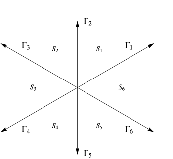
Any solution of (204a) is an entire function of $\zeta$ . Let $S_{j},j=1,\ldots,6$ denote the sectors

S_{j}=\biggl{\{}\zeta\in\mathbb{C}\dvtx\frac{2j-3}{6}\pi<\arg(\zeta)<\frac{2j-1}{6}\pi\biggr{\}},

(205)

and let $\Gamma_{j}$ denote the outwardly oriented boundary rays (see Figure 9)

\Gamma_{j}=\biggl{\{}\zeta\in\mathbb{C}\dvtx\arg(\zeta)=\frac{2j-1}{6}\pi\biggr{\}}.

(206)

There exists a unique solution $\Psi_{j}$ of (204a) such that

\Psi_{j}=I+\mathcal{O}\bigl{(}\zeta^{-1}\bigr{)}\qquad\mbox{as }\zeta\to\infty\mbox{ in }S_{j},

(207)

and constants $a_{j},j=1,\ldots,6$ such that for $\zeta\in\Gamma_{j}$

	$\displaystyle\Psi_{j+1}(\zeta)$	$\displaystyle=$	$\displaystyle\Psi_{j}(\zeta)\pmatrix{1&0\vskip 2.0pt\cr a_{j}e^{-2i(({4}/{3})\zeta^{3}+s\zeta)}&1},\qquad j\mbox{ odd, }$
	$\displaystyle\Psi_{j+1}(\zeta)$	$\displaystyle=$	$\displaystyle\Psi_{j}(\zeta)\pmatrix{1&a_{j}e^{2i(({4}/{3})\zeta^{3}+s\zeta)}\vskip 2.0pt\cr 0&1},\qquad j\mbox{ even.}$

Additionally, the constants $a_{j}$ satisfy

a_{j+3}=a_{j},\qquad a_{1}a_{2}a_{3}+a_{1}+a_{2}+a_{3}=0.

(209)

The parameters $a_{j}$ depend parametrically on $s,q$ and $r$ ; in FN76 Flaschka and Newell showed that the isomonodromic deformations, that is, the variations of these parameters that keep the Stokes multipliers $a_{j}$ constant, are given by solutions of the Painlevé II equation $q^{\prime\prime}(s)=sq+2q(s)^{3}$ and $r(s)=q^{\prime}(s)$ .

Our particular interest is in the Hastings–McLeod solution of Painlevé II HM , which is the unique solution such that

	$\displaystyle q(s)$	$\displaystyle=$	$\displaystyle\operatorname{Ai}(s)\bigl{(}1+{o}(1)\bigr{)}\qquad\mbox{as }s\to\infty,$
	$\displaystyle q(s)$	$\displaystyle\sim$	$\displaystyle\sqrt{-\frac{s}{2}}\qquad\mbox{as }s\to-\infty.$

Let $\Psi(\zeta;s)$ be the solution of (204a) with parameters $s,q=q(s)$ and $r=q^{\prime}(s)$ , where $q(s)$ is the Hastings–McLeod solution, and let $\mathcal{P}$ denote the set of poles of $q$ (of which there are infinitely many). Then $\bolds{\Psi}(\zeta,s)$ is defined and analytic for $\zeta\in\mathbb{C}\setminus(C_{1}\cup C_{2})$ and $s\in\mathbb{C}\setminus\mathcal{P}$ . It is known that there are no poles of $q$ on the real line HM . The Stokes multiplier for the Hastings–McLeod solution are

a_{1}=1,\qquad a_{2}=0,\qquad a_{3}=-1.

(211)

If we reverse the orientation of $\Gamma_{3}$ and $\Gamma_{4}$ and define $C_{1}=\Gamma_{1}\cup\Gamma_{3}$ and $C_{2}=\Gamma_{4}\cup\Gamma_{6}$ (see Figure 10), then $\Psi(\zeta;s)$ solves the following RHP:

Riemann–Hilbert Problem 10.1 ((PII model RHP)).

Find a $2\times 2$ matrix $\Psi(\zeta;s)$ with the following properties: {longlist}[(1)]

$\Psi(\zeta;s)$ is an analytic function of $\zeta$ for $\zeta\in\mathbb{C}\setminus(C_{1}\cup C_{2})$ .

$\Psi(\zeta;s)=I+\mathcal{O}(\zeta^{-1})$ as $\zeta\to\infty$ and bounded as $\zeta\to 0$ .

The boundary values $\Psi_{\pm}(\zeta;s)$ satisfy the jump conditions

\displaystyle\cases{\displaystyle\Psi_{+}(\zeta;s)=\Psi_{-}(\zeta;s)\pmatrix{1&0\vskip 2.0pt\cr e^{2i\theta_{\mathit{PII}}}&1},&\quad$\zeta\in C_{1},$\vskip 3.0pt\cr\displaystyle\Psi_{+}(\zeta;s)=\Psi_{-}(\zeta;s)\pmatrix{1&-e^{-2i\theta_{\mathit{PII}}}\vskip 2.0pt\cr 0&1},&\quad$\zeta\in C_{2},$}

(212)

where

\theta_{\mathit{PII}}=\theta_{\mathit{PII}}(\zeta,s)=\tfrac{4}{3}\zeta^{3}+s\zeta.

(213)

We make two observations which we will need later. First, the symmetries $-C_{1}=C_{2}$ and $\theta_{\mathit{PII}}(-\zeta,s)=-\theta_{\mathit{PII}}(\zeta,s)$ imply that the solution $\Psi(\zeta,s)$ of RHP 10.1 satisfies the symmetry

\displaystyle\Psi(-\zeta,s)=\sigma_{1}\Psi(\zeta,s)\sigma_{1},\qquad\sigma_{1}:=\left(\matrix{0&1\cr 1&0}\right).

(214)

The second fact is that $\Psi$ admits a uniformly expansion in the limit as $\zeta\to\infty$ as described in DZ95 . Specifically, we have

\Psi(\zeta;s)=I+\frac{\psi_{1}(s)}{\zeta}+\frac{\psi_{2}(s)}{\zeta^{2}}+\frac{\psi_{3}(s)}{\zeta^{3}}+\mathcal{O}\bigl{(}\zeta^{-4}\bigr{)}.

(215)

The error term $\mathcal{O}(\zeta^{-4})$ here depends on $s$ . For our purpose, we need the dependence on $s$ for $s$ bounded below. An analysis similar to Section 6 of DZ95 shows that given $s_{0}>0$ , there exists a constant $c_{0}>0$ such that

	$\Psi(\zeta;s)=I+\frac{\psi_{1}(s)}{\zeta}+\frac{\psi_{2}(s)}{\zeta^{2}}+\frac{\psi_{3}(s)}{\zeta^{3}}+\mathcal{O}\biggl{(}\frac{e^{-c_{0}\|s\|^{3/2}}}{\zeta^{4}}\biggr{)}.$			(216a)
The moments $\psi_{j}(s)$ can be calculated recursively from inserting the expansion into (204b). The first three moments are

	$\displaystyle\psi_{1}(s)$	$\displaystyle=$	$\displaystyle\frac{1}{2i}\left[\matrix{-u(s)&q(s)\cr-q(s)&u(s)}\right],$
	$\displaystyle\psi_{2}(s)$	$\displaystyle=$	$\displaystyle\frac{1}{(2i)^{2}}\left[\matrix{\frac{1}{2}u(s)^{2}-\frac{1}{2}q(s)^{2}&q(s)u(s)-q^{\prime}(s)\cr q(s)u(s)-q^{\prime}(s)&\frac{1}{2}u(s)^{2}-\frac{1}{2}q(s)^{2}}\right],$	(216b)
	$\displaystyle\psi_{3}(s)$	$\displaystyle=$	$\displaystyle\frac{1}{(2i)^{3}}\left[\matrix{\alpha(s)&-\beta(s)\cr\beta(s)&-\alpha(s)}\right],$
where

	$\displaystyle u(s)$	$\displaystyle=$	$\displaystyle\int_{\infty}^{s}q(\xi)^{2}\,d\xi,$	(216c)
	$\displaystyle\alpha(s)$	$\displaystyle=$	$\displaystyle\frac{q(s)^{2}u(s)}{2}-\frac{u(s)^{3}}{6}+\log F(s)^{2}-\int_{\infty}^{s}q^{\prime}(\xi)^{2}\,d\xi,$	(216d)
	$\displaystyle\beta(s)$	$\displaystyle=$	$\displaystyle q^{\prime}(s)u(s)-q(s)\biggl{(}s+\frac{q(s)^{2}}{2}+\frac{u(s)^{2}}{2}\biggr{)}.$	(216e)

We note that the asymptotic analysis of the RHP for the Painlevé equation implies that for a given $s_{0}>0$ ,

\displaystyle\psi_{j}(s)=\mathcal{O}\bigl{(}e^{-c_{0}|s|^{3/2}}\bigr{)},\qquad j=1,2,3,

(217)

where $c_{0}$ can be taken as the same constant in the error term of (216a).

Acknowledgments

J. B. would like to thank Mishko Mitkovshi for bringing his attention to the paper of Chen, Deng, Du, Stanley and Yan during the summer graduate workshop at MSRI. This initiated this paper. We would also like the thank Christian Krattenthaler, Peter Miller, Richard Stanley, Craig Tracy and Catherine Yan for helpful communications.

References

(1) {bmisc}[auto:STB—2012/12/19—13:34:42] \bauthor\bsnmAdler, \bfnmM.\binitsM., \bauthor\bsnmFerrari, \bfnmP. L.\binitsP. L. and \bauthor\bparticlevan \bsnmMoerbeke, \bfnmP.\binitsP. (\byear2010). \bhowpublishedNon-intersecting random walks in the neighborhood of a symmetric tacnode. Available at arXiv:\arxivurl1007.1163. \bptokimsref \endbibitem
(2) {barticle}[mr] \bauthor\bsnmBaik, \bfnmJinho\binitsJ., \bauthor\bsnmBorodin, \bfnmAlexei\binitsA., \bauthor\bsnmDeift, \bfnmPercy\binitsP. and \bauthor\bsnmSuidan, \bfnmToufic\binitsT. (\byear2006). \btitleA model for the bus system in Cuernavaca (Mexico). \bjournalJ. Phys. A \bvolume39 \bpages8965–8975. \biddoi=10.1088/0305-4470/39/28/S11, issn=0305-4470, mr=2240467 \bptokimsref \endbibitem
(3) {barticle}[mr] \bauthor\bsnmBaik, \bfnmJinho\binitsJ., \bauthor\bsnmBuckingham, \bfnmRobert\binitsR. and \bauthor\bsnmDiFranco, \bfnmJeffery\binitsJ. (\byear2008). \btitleAsymptotics of Tracy–Widom distributions and the total integral of a Painlevé II function. \bjournalComm. Math. Phys. \bvolume280 \bpages463–497. \biddoi=10.1007/s00220-008-0433-5, issn=0010-3616, mr=2395479 \bptokimsref \endbibitem
(4) {barticle}[mr] \bauthor\bsnmBaik, \bfnmJinho\binitsJ., \bauthor\bsnmDeift, \bfnmPercy\binitsP. and \bauthor\bsnmJohansson, \bfnmKurt\binitsK. (\byear1999). \btitleOn the distribution of the length of the longest increasing subsequence of random permutations. \bjournalJ. Amer. Math. Soc. \bvolume12 \bpages1119–1178. \biddoi=10.1090/S0894-0347-99-00307-0, issn=0894-0347, mr=1682248 \bptokimsref \endbibitem
(5) {barticle}[mr] \bauthor\bsnmBaik, \bfnmJinho\binitsJ., \bauthor\bsnmDeift, \bfnmPercy\binitsP. and \bauthor\bsnmRains, \bfnmEric\binitsE. (\byear2001). \btitleA Fredholm determinant identity and the convergence of moments for random Young tableaux. \bjournalComm. Math. Phys. \bvolume223 \bpages627–672. \biddoi=10.1007/s002200100555, issn=0010-3616, mr=1866169 \bptokimsref \endbibitem
(6) {bbook}[mr] \bauthor\bsnmBaik, \bfnmJ.\binitsJ., \bauthor\bsnmKriecherbauer, \bfnmT.\binitsT., \bauthor\bsnmMcLaughlin, \bfnmK. T. R.\binitsK. T. R. and \bauthor\bsnmMiller, \bfnmP. D.\binitsP. D. (\byear2007). \btitleDiscrete Orthogonal Polynomials: Asymptotics and Applications. \bseriesAnnals of Mathematics Studies \bvolume164. \bpublisherPrinceton Univ. Press, \blocationPrinceton, NJ. \bidmr=2283089 \bptokimsref \endbibitem
(7) {bmisc}[auto:STB—2012/12/19—13:34:42] \bauthor\bsnmBaik, \bfnmJ.\binitsJ. and \bauthor\bsnmLiu, \bfnmZ.\binitsZ. (\byear2013). \bhowpublishedDiscrete Topelitz/Hankel determinants and the width of non-intersecting processes. Available at \arxivurlarXiv:1212.4467. \bptokimsref \endbibitem
(8) {barticle}[mr] \bauthor\bsnmBaik, \bfnmJinho\binitsJ. and \bauthor\bsnmRains, \bfnmEric M.\binitsE. M. (\byear2001). \btitleAlgebraic aspects of increasing subsequences. \bjournalDuke Math. J. \bvolume109 \bpages1–65. \biddoi=10.1215/S0012-7094-01-10911-3, issn=0012-7094, mr=1844203 \bptokimsref \endbibitem
(9) {barticle}[mr] \bauthor\bsnmBaik, \bfnmJinho\binitsJ. and \bauthor\bsnmRains, \bfnmEric M.\binitsE. M. (\byear2001). \btitleThe asymptotics of monotone subsequences of involutions. \bjournalDuke Math. J. \bvolume109 \bpages205–281. \biddoi=10.1215/S0012-7094-01-10921-6, issn=0012-7094, mr=1845180 \bptokimsref \endbibitem
(10) {barticle}[mr] \bauthor\bsnmBasor, \bfnmEstelle L.\binitsE. L. and \bauthor\bsnmEhrhardt, \bfnmTorsten\binitsT. (\byear2009). \btitleDeterminant computations for some classes of Toeplitz–Hankel matrices. \bjournalOper. Matrices \bvolume3 \bpages167–186. \biddoi=10.7153/oam-03-09, issn=1846-3886, mr=2522773 \bptokimsref \endbibitem
(11) {barticle}[mr] \bauthor\bsnmBornemann, \bfnmFolkmar\binitsF. (\byear2010). \btitleAsymptotic independence of the extreme eigenvalues of Gaussian unitary ensemble. \bjournalJ. Math. Phys. \bvolume51 \bpages023514, 8. \biddoi=10.1063/1.3290968, issn=0022-2488, mr=2605065 \bptokimsref \endbibitem
(12) {barticle}[mr] \bauthor\bsnmBornemann, \bfnmF.\binitsF. (\byear2010). \btitleOn the numerical evaluation of distributions in random matrix theory: A review. \bjournalMarkov Process. Related Fields \bvolume16 \bpages803–866. \bidissn=1024-2953, mr=2895091 \bptokimsref \endbibitem
(13) {bbook}[mr] \bauthor\bsnmBöttcher, \bfnmAlbrecht\binitsA. and \bauthor\bsnmKarlovich, \bfnmYuri I.\binitsY. I. (\byear1997). \btitleCarleson Curves, Muckenhoupt Weights, and Toeplitz Operators. \bseriesProgress in Mathematics \bvolume154. \bpublisherBirkhäuser, \blocationBasel. \biddoi=10.1007/978-3-0348-8922-3, mr=1484165 \bptokimsref \endbibitem
(14) {barticle}[mr] \bauthor\bsnmBuckingham, \bfnmRobert J.\binitsR. J. and \bauthor\bsnmMiller, \bfnmPeter D.\binitsP. D. (\byear2012). \btitleThe sine-Gordon equation in the semiclassical limit: Critical behavior near a separatrix. \bjournalJ. Anal. Math. \bvolume118 \bpages397–492. \biddoi=10.1007/s11854-012-0041-3, issn=0021-7670, mr=3000688 \bptnotecheck year\bptokimsref \endbibitem
(15) {barticle}[mr] \bauthor\bsnmChen, \bfnmWilliam Y. C.\binitsW. Y. C., \bauthor\bsnmDeng, \bfnmEva Y. P.\binitsE. Y. P., \bauthor\bsnmDu, \bfnmRosena R. X.\binitsR. R. X., \bauthor\bsnmStanley, \bfnmRichard P.\binitsR. P. and \bauthor\bsnmYan, \bfnmCatherine H.\binitsC. H. (\byear2007). \btitleCrossings and nestings of matchings and partitions. \bjournalTrans. Amer. Math. Soc. \bvolume359 \bpages1555–1575. \biddoi=10.1090/S0002-9947-06-04210-3, issn=0002-9947, mr=2272140 \bptokimsref \endbibitem
(16) {barticle}[mr] \bauthor\bsnmChester, \bfnmC.\binitsC., \bauthor\bsnmFriedman, \bfnmB.\binitsB. and \bauthor\bsnmUrsell, \bfnmF.\binitsF. (\byear1957). \btitleAn extension of the method of steepest descents. \bjournalMath. Proc. Cambridge Philos. Soc. \bvolume53 \bpages599–611. \bidmr=0090690 \bptokimsref \endbibitem
(17) {barticle}[mr] \bauthor\bsnmChoup, \bfnmLeonard N.\binitsL. N. (\byear2006). \btitleEdgeworth expansion of the largest eigenvalue distribution function of GUE and LUE. \bjournalInt. Math. Res. Not. IMRN \bpagesArt. ID 61049, 32. \biddoi=10.1155/IMRN/2006/61049, issn=1073-7928, mr=2233711 \bptokimsref \endbibitem
(18) {barticle}[mr] \bauthor\bsnmChoup, \bfnmLeonard N.\binitsL. N. (\byear2008). \btitleEdgeworth expansion of the largest eigenvalue distribution function of Gaussian unitary ensemble revisited. \bjournalJ. Math. Phys. \bvolume49 \bpages033508, 16. \biddoi=10.1063/1.2873345, issn=0022-2488, mr=2406805 \bptokimsref \endbibitem
(19) {barticle}[mr] \bauthor\bsnmClaeys, \bfnmTom\binitsT. and \bauthor\bsnmKuijlaars, \bfnmArno B. J.\binitsA. B. J. (\byear2006). \btitleUniversality of the double scaling limit in random matrix models. \bjournalComm. Pure Appl. Math. \bvolume59 \bpages1573–1603. \biddoi=10.1002/cpa.20113, issn=0010-3640, mr=2254445 \bptokimsref \endbibitem
(20) {barticle}[auto:STB—2012/12/19—13:34:42] \bauthor\bsnmCorwin, \bfnmI.\binitsI., \bauthor\bsnmQuastel, \bfnmJ.\binitsJ. and \bauthor\bsnmRemenik, \bfnmD.\binitsD. (\byear2013). \btitleContinuum statistics of the Airy2 process. \bjournalComm. Math. Phys. \bvolume317 \bpages347–362. \bptokimsref \endbibitem
(21) {barticle}[mr] \bauthor\bsnmDeift, \bfnmP.\binitsP., \bauthor\bsnmKriecherbauer, \bfnmT.\binitsT., \bauthor\bsnmMcLaughlin, \bfnmK. T. R.\binitsK. T. R., \bauthor\bsnmVenakides, \bfnmS.\binitsS. and \bauthor\bsnmZhou, \bfnmX.\binitsX. (\byear1999). \btitleStrong asymptotics of orthogonal polynomials with respect to exponential weights. \bjournalComm. Pure Appl. Math. \bvolume52 \bpages1491–1552. \biddoi=10.1002/(SICI)1097-0312(199912)52:12<1491::AID-CPA2>3.3.CO;2-R , issn=0010-3640, mr=1711036 \bptokimsref \endbibitem
(22) {barticle}[mr] \bauthor\bsnmDeift, \bfnmP.\binitsP., \bauthor\bsnmKriecherbauer, \bfnmT.\binitsT., \bauthor\bsnmMcLaughlin, \bfnmK. T. R.\binitsK. T. R., \bauthor\bsnmVenakides, \bfnmS.\binitsS. and \bauthor\bsnmZhou, \bfnmX.\binitsX. (\byear1999). \btitleUniform asymptotics for polynomials orthogonal with respect to varying exponential weights and applications to universality questions in random matrix theory. \bjournalComm. Pure Appl. Math. \bvolume52 \bpages1335–1425. \biddoi=10.1002/(SICI)1097-0312(199911)52:11<1335::AID-CPA1>3.0.CO;2-1 , issn=0010-3640, mr=1702716 \bptokimsref \endbibitem
(23) {barticle}[mr] \bauthor\bsnmDeift, \bfnmP. A.\binitsP. A. and \bauthor\bsnmZhou, \bfnmX.\binitsX. (\byear1995). \btitleAsymptotics for the Painlevé II equation. \bjournalComm. Pure Appl. Math. \bvolume48 \bpages277–337. \biddoi=10.1002/cpa.3160480304, issn=0010-3640, mr=1322812 \bptokimsref \endbibitem
(24) {barticle}[mr] \bauthor\bsnmEl Karoui, \bfnmNoureddine\binitsN. (\byear2006). \btitleA rate of convergence result for the largest eigenvalue of complex white Wishart matrices. \bjournalAnn. Probab. \bvolume34 \bpages2077–2117. \biddoi=10.1214/009117906000000502, issn=0091-1798, mr=2294977 \bptokimsref \endbibitem
(25) {barticle}[mr] \bauthor\bsnmFerrari, \bfnmPatrik L.\binitsP. L. and \bauthor\bsnmFrings, \bfnmRené\binitsR. (\byear2011). \btitleFinite time corrections in KPZ growth models. \bjournalJ. Stat. Phys. \bvolume144 \bpages1123–1150. \biddoi=10.1007/s10955-011-0318-4, issn=0022-4715, mr=2841918 \bptokimsref \endbibitem
(26) {barticle}[mr] \bauthor\bsnmFlaschka, \bfnmHermann\binitsH. and \bauthor\bsnmNewell, \bfnmAlan C.\binitsA. C. (\byear1980). \btitleMonodromy- and spectrum-preserving deformations. I. \bjournalComm. Math. Phys. \bvolume76 \bpages65–116. \bidissn=0010-3616, mr=0588248 \bptokimsref \endbibitem
(27) {barticle}[mr] \bauthor\bsnmFokas, \bfnmA. S.\binitsA. S., \bauthor\bsnmIts, \bfnmA. R.\binitsA. R. and \bauthor\bsnmKitaev, \bfnmA. V.\binitsA. V. (\byear1992). \btitleThe isomonodromy approach to matrix models in $2$ D quantum gravity. \bjournalComm. Math. Phys. \bvolume147 \bpages395–430. \bidissn=0010-3616, mr=1174420 \bptokimsref \endbibitem
(28) {barticle}[mr] \bauthor\bsnmFriedman, \bfnmB.\binitsB. (\byear1959). \btitleStationary phase with neighboring critical points. \bjournalJ. Soc. Indust. Appl. Math. \bvolume7 \bpages280–289. \bidmr=0109272 \bptokimsref \endbibitem
(29) {barticle}[mr] \bauthor\bsnmGessel, \bfnmIra M.\binitsI. M. (\byear1990). \btitleSymmetric functions and P-recursiveness. \bjournalJ. Combin. Theory Ser. A \bvolume53 \bpages257–285. \biddoi=10.1016/0097-3165(90)90060-A, issn=0097-3165, mr=1041448 \bptokimsref \endbibitem
(30) {barticle}[mr] \bauthor\bsnmGolinskiĭ, \bfnmL. B.\binitsL. B. (\byear2006). \btitleSchur flows and orthogonal polynomials on the unit circle. \bjournalMat. Sb. \bvolume197 \bpages41–62. \biddoi=10.1070/SM2006v197n08ABEH003792, issn=0368-8666, mr=2272777 \bptokimsref \endbibitem
(31) {barticle}[mr] \bauthor\bsnmGrabiner, \bfnmDavid J.\binitsD. J. (\byear1999). \btitleBrownian motion in a Weyl chamber, non-colliding particles, and random matrices. \bjournalAnn. Inst. Henri Poincaré Probab. Stat. \bvolume35 \bpages177–204. \biddoi=10.1016/S0246-0203(99)80010-7, issn=0246-0203, mr=1678525 \bptokimsref \endbibitem
(32) {barticle}[mr] \bauthor\bsnmHastings, \bfnmS. P.\binitsS. P. and \bauthor\bsnmMcLeod, \bfnmJ. B.\binitsJ. B. (\byear1980). \btitleA boundary value problem associated with the second Painlevé transcendent and the Korteweg–de Vries equation. \bjournalArch. Ration. Mech. Anal. \bvolume73 \bpages31–51. \biddoi=10.1007/BF00283254, issn=0003-9527, mr=0555581 \bptokimsref \endbibitem
(33) {barticle}[mr] \bauthor\bsnmJohansson, \bfnmKurt\binitsK. (\byear1998). \btitleThe longest increasing subsequence in a random permutation and a unitary random matrix model. \bjournalMath. Res. Lett. \bvolume5 \bpages63–82. \bidissn=1073-2780, mr=1618351 \bptokimsref \endbibitem
(34) {barticle}[mr] \bauthor\bsnmJohansson, \bfnmKurt\binitsK. (\byear2002). \btitleNon-intersecting paths, random tilings and random matrices. \bjournalProbab. Theory Related Fields \bvolume123 \bpages225–280. \biddoi=10.1007/s004400100187, issn=0178-8051, mr=1900323 \bptokimsref \endbibitem
(35) {barticle}[mr] \bauthor\bsnmJohansson, \bfnmKurt\binitsK. (\byear2003). \btitleDiscrete polynuclear growth and determinantal processes. \bjournalComm. Math. Phys. \bvolume242 \bpages277–329. \bidissn=0010-3616, mr=2018275 \bptokimsref \endbibitem
(36) {barticle}[mr] \bauthor\bsnmJohansson, \bfnmKurt\binitsK. (\byear2005). \btitleThe arctic circle boundary and the Airy process. \bjournalAnn. Probab. \bvolume33 \bpages1–30. \biddoi=10.1214/009117904000000937, issn=0091-1798, mr=2118857 \bptokimsref \endbibitem
(37) {barticle}[mr] \bauthor\bsnmJohnstone, \bfnmIain M.\binitsI. M. (\byear2008). \btitleMultivariate analysis and Jacobi ensembles: Largest eigenvalue, Tracy–Widom limits and rates of convergence. \bjournalAnn. Statist. \bvolume36 \bpages2638–2716. \biddoi=10.1214/08-AOS605, issn=0090-5364, mr=2485010 \bptokimsref \endbibitem
(38) {bmisc}[auto:STB—2012/12/19—13:34:42] \bauthor\bsnmJohnstone, \bfnmI. M.\binitsI. M. and \bauthor\bsnmMa, \bfnmZ.\binitsZ. (\byear2011). \bhowpublishedFast approach to the Tracy–Widom law at the edge of GOE and GUE. Available at arXiv:\arxivurl1110.0108. \bptokimsref \endbibitem
(39) {bbook}[mr] \bauthor\bsnmKamvissis, \bfnmSpyridon\binitsS., \bauthor\bsnmMcLaughlin, \bfnmKenneth D. T. R.\binitsK. D. T. R. and \bauthor\bsnmMiller, \bfnmPeter D.\binitsP. D. (\byear2003). \btitleSemiclassical Soliton Ensembles for the Focusing Nonlinear Schrödinger Equation. \bseriesAnnals of Mathematics Studies \bvolume154. \bpublisherPrinceton Univ. Press, \blocationPrinceton, NJ. \bidmr=1999840 \bptokimsref \endbibitem
(40) {barticle}[mr] \bauthor\bsnmKarlin, \bfnmSamuel\binitsS. and \bauthor\bsnmMcGregor, \bfnmJames\binitsJ. (\byear1959). \btitleCoincidence probabilities. \bjournalPacific J. Math. \bvolume9 \bpages1141–1164. \bidissn=0030-8730, mr=0114248 \bptokimsref \endbibitem
(41) {barticle}[mr] \bauthor\bsnmKönig, \bfnmWolfgang\binitsW., \bauthor\bsnmO’Connell, \bfnmNeil\binitsN. and \bauthor\bsnmRoch, \bfnmSébastien\binitsS. (\byear2002). \btitleNon-colliding random walks, tandem queues, and discrete orthogonal polynomial ensembles. \bjournalElectron. J. Probab. \bvolume7 \bpages24 pp. (electronic). \bidissn=1083-6489, mr=1887625 \bptokimsref \endbibitem
(42) {barticle}[mr] \bauthor\bsnmKrattenthaler, \bfnmC.\binitsC. (\byear2006). \btitleGrowth diagrams, and increasing and decreasing chains in fillings of Ferrers shapes. \bjournalAdv. in Appl. Math. \bvolume37 \bpages404–431. \biddoi=10.1016/j.aam.2005.12.006, issn=0196-8858, mr=2261181 \bptokimsref \endbibitem
(43) {barticle}[mr] \bauthor\bsnmMa, \bfnmZongming\binitsZ. (\byear2012). \btitleAccuracy of the Tracy–Widom limits for the extreme eigenvalues in white Wishart matrices. \bjournalBernoulli \bvolume18 \bpages322–359. \biddoi=10.3150/10-BEJ334, issn=1350-7265, mr=2888709 \bptokimsref \endbibitem
(44) {barticle}[mr] \bauthor\bsnmMoreno Flores, \bfnmG.\binitsG., \bauthor\bsnmQuastel, \bfnmJ.\binitsJ. and \bauthor\bsnmRemenik, \bfnmD.\binitsD. (\byear2013). \btitleEndpoint distribution of directed polymers in $1+1$ dimensions. \bjournalComm. Math. Phys. \bvolume317 \bpages363–380. \bptokimsref \endbibitem
(45) {barticle}[mr] \bauthor\bsnmNenciu, \bfnmIrina\binitsI. (\byear2005). \btitleLax pairs for the Ablowitz–Ladik system via orthogonal polynomials on the unit circle. \bjournalInt. Math. Res. Not. IMRN \bvolume11 \bpages647–686. \biddoi=10.1155/IMRN.2005.647, issn=1073-7928, mr=2146324 \bptokimsref \endbibitem
(46) {barticle}[mr] \bauthor\bsnmRains, \bfnmE. M.\binitsE. M. (\byear1998). \btitleIncreasing subsequences and the classical groups. \bjournalElectron. J. Combin. \bvolume5 \bpagesResearch Paper 12, 9 pp. (electronic). \bidissn=1077-8926, mr=1600095 \bptokimsref \endbibitem
(47) {barticle}[mr] \bauthor\bsnmShinault, \bfnmGregory\binitsG. and \bauthor\bsnmTracy, \bfnmCraig A.\binitsC. A. (\byear2011). \btitleAsymptotics for the covariance of the $\mathrm{Airy}_{2}$ process. \bjournalJ. Stat. Phys. \bvolume143 \bpages60–71. \biddoi=10.1007/s10955-011-0155-5, issn=0022-4715, mr=2787973 \bptokimsref \endbibitem
(48) {bincollection}[mr] \bauthor\bsnmStanley, \bfnmRichard P.\binitsR. P. (\byear2007). \btitleIncreasing and decreasing subsequences and their variants. In \bbooktitleInternational Congress of Mathematicians. Vol. I \bpages545–579. \bpublisherEur. Math. Soc., \blocationZürich. \biddoi=10.4171/022-1/21, mr=2334203 \bptokimsref \endbibitem
(49) {bbook}[mr] \bauthor\bsnmSzegő, \bfnmGábor\binitsG. (\byear1975). \btitleOrthogonal Polynomials, \bedition4th ed. \bpublisherAmer. Math. Soc., \blocationProvidence, RI. \bidmr=0372517 \bptokimsref \endbibitem
(50) {barticle}[mr] \bauthor\bsnmTracy, \bfnmCraig A.\binitsC. A. and \bauthor\bsnmWidom, \bfnmHarold\binitsH. (\byear1996). \btitleOn orthogonal and symplectic matrix ensembles. \bjournalComm. Math. Phys. \bvolume177 \bpages727–754. \bidissn=0010-3616, mr=1385083 \bptokimsref \endbibitem

Limiting distribution of maximal crossing and nesting of Poissonized random matchings

Abstract

doi:

keywords:

keywords:

1 Introduction

1.1 Joint distribution

Theorem 1.1.

Corollary 1.1.

Corollary 1.2.

1.2 Marginal distribution

Theorem 1.2.

1.3 Toeplitz minus Hankel with a discrete symbol

Proposition 1.1.

1.4 Longest increasing subsequence of random permutation

Theorem 1.3.

1.5 Organization of paper

2 Height and depth of nonintersecting continuous-time simple random walks

Lemma 2.1.

3 Proof of Proposition 1.1

4 Orthogonal polynomial Riemann–Hilbert problems

Riemann–Hilbert Problem 4.1 (for discrete OPs).

Riemann–Hilbert Problem 4.2 (for continuous OPs).

5 The exponentially small regime

Riemann–Hilbert Problem 5.1 (for Q(z)).

Riemann–Hilbert Problem 5.2 (for S​(z)S(z)).

Riemann–Hilbert Problem 5.3 (for T(z)).

Proposition 5.1.

6 Painlevé regime

6.1 Local models near 11 and −1-1

Riemann–Hilbert Problem 6.1 (for 𝐑​(z)\mathbf{R}(z)).

6.2 Analysis of the continuous weight problem

6.3 Expansion of 𝐑​(0)\mathbf{R}(0)

Proposition 6.1.

Proposition 6.2.

7 Proof of Theorem 1.1 and Corollary 1.1

8 Proof of Theorems 1.2 and 1.3

9 Proof of Corollary 1.2

Lemma 9.1.

10 A model RHP: Painlevé II

Riemann–Hilbert Problem 10.1 ((PII model RHP)).

Acknowledgments

References

Riemann–Hilbert Problem 5.2 (for $S(z)$ ).

6.1 Local models near $1$ and $-1$

Riemann–Hilbert Problem 6.1 (for $\mathbf{R}(z)$ ).

6.3 Expansion of $\mathbf{R}(0)$