Limiting distributions of ratios of Binomial random variables
Abstract
We consider the limiting distribution of the quantity , where and are two independent Binomial random variables with a common success probability and a number of trials and , respectively, and are positive real numbers. Under several settings, we prove that this converges to a Normal distribution with a given mean and variance, and demonstrate these theoretical results through simulations.
1 Introduction
As part of the analysis in lubberts2025 , the authors consider the quantity
where , and are independent of one another. The setting of interest in that paper occurs when has order comparable to , so that the quantity in the denominator is typically of a similar order to the one in the numerator, and in this case, it was shown that for large values of , this ratio has a limiting Normal distribution with mean and variance . While it is well-known that given the value of , for some random variables and as above, the value of is a Hypergeometric random variable, the literature is less forthcoming about the distribution of such ratios of a pair of Binomial random variables. In the present work, we extend the previous results to the case where the function takes the form
for . We will show that under several parameter regimes, has a limiting Normal distribution. We verify these results through simulations, showing the effects of varying each of the parameters on the observed distribution.
2 Limiting Distribution
We may approximate the function defining our ratio of interest using the Taylor approximation:
| (1) |
where the quadratic remainder term takes the form
for some point on the line segment connecting with .
If we substitute the random variables and into this expression, the linear term in Equation (1) already looks quite Normal in distribution once and are large, since are independent Binomial random variables. However, in order to show that the limiting distribution of looks like the linear terms in this equation, we must bound the remainder term. We will make use of the following result from chung2000course :
Lemma 1.
Let in distribution, and in probability. Then in distribution.
We will show that after appropriate scaling, the quadratic remainder term converges to 0 in probability, so the two linear terms determine the limiting distribution of . For any quadratic form , applying the Cauchy-Schwarz inequality and monotonicity property of the spectral norm, we have
so in order to control we must find an upper bound for . Note that a Hessian matrix must be symmetric, so its singular values are simply the absolute values of its eigenvalues. The Gerschgorin disk theorem horn2012matrix tells us that any eigenvalue of a matrix must belong to the union of its Gerschgorin disks, so no eigenvalue of a matrix can be larger than
In the present case, the Hessian is given by
Utilizing the Gerschgorin bound just stated, we have
| (2) |
Now since are Binomial random variables, we know that with overwhelming probability, , and ; let us call this event . More precisely, the probability that decays faster than , and similarly for . So to bound the residual term, we see that the event
and thus
Consider , where , and , where . Then the right hand side of inequality (2) may be bounded by
We also have the inequality
so on the event , we get that
| (3) |
since are constants. The exact behavior of this quantity depends on the ratio , but in light of Lemma 1, in order to obtain the distributional convergence results, we must simply show that the final quantity in (3) still goes to zero after appropriate scaling, for any of the cases we wish to consider.
To find the limiting distribution of , we re-arrange Equation (1) after evaluating at (and neglecting the remainder term for the time being):
The last vector will converge to a Normal vector as , but an appropriate scaling is required so that neither of the coefficients of diverge as , and it is not the case that both of them vanish (since in that case, the limiting distribution is simply point mass at 0). The choice of scaling will again depend on the ratio , but now we have all of the ingredients in place to prove the following theorem:
Theorem 1.
Let , be constants. Let , and let be independent of . Define
Then as , we have the following convergences in distribution:
-
(i)
If , , then
-
(ii)
If , then
-
(iii)
If , then
Proof.
It remains to be shown that in the three cases described above, the bound in (3) still goes to zero after multiplication by the appropriate scaling factor as .
-
(i)
When , , then
-
(ii)
When , then
-
(iii)
When , then
∎
3 Simulation
We verify our limiting distribution results for different values of the parameters , and . For each set of parameter values we tested, we generate 100,000 points , where , , and are independent. We then compute , and center and scale according to Theorem 1, obtaining . We compare this sample with a sample of 100,000 values drawn from the Normal distribution with mean 0 and the appropriate variance. To measure the accuracy between the distributions of and , we use the discrete KL divergence: We divide the values in into 100 bins , then set to be the observed proportion of and to be the observed proportion of . We compare the two distributions with the formula
| (4) |
When , it can happen that all of the observations fall into a single bin, so in this case we use the reversed formula to get a meaningful comparison of the distributions:
| (5) |
We test the distributions in each of the settings of Theorem 1, as well as the case where , but . Whenever we fix the value of or , it is set equal to 15 (except in Section 3.4, for reasons that we explain there), and whenever we fix the value of , it is set equal to 0.5. For each of the regimes of , all plots show the effect of varying one of the parameters while the others remain fixed.
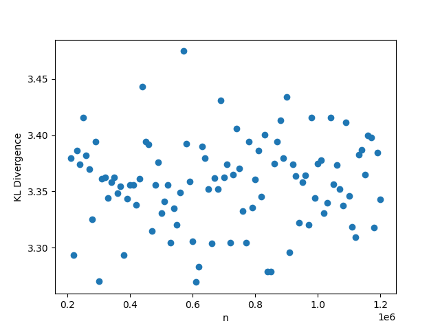
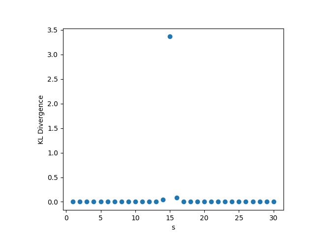
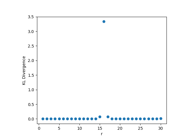
3.1
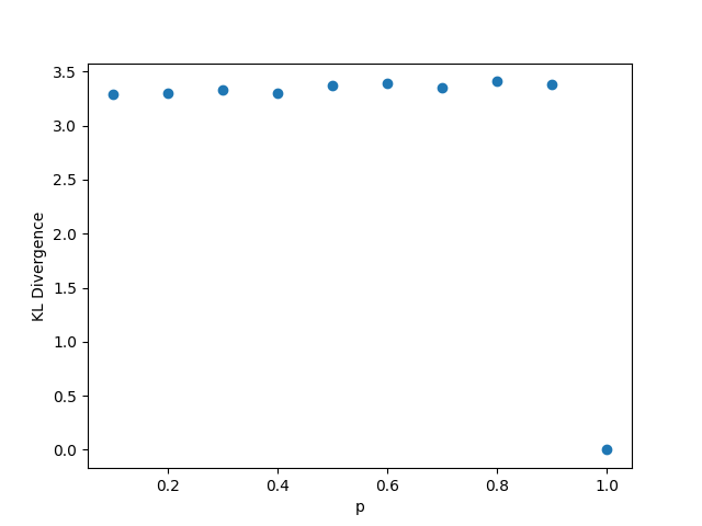
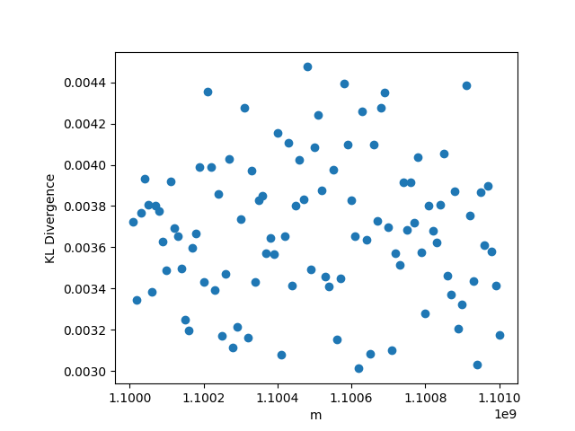
While outside the scope of the theorem, for this setting, whenever we fix or , we choose , . Whenever we fix one of , we set its value to be , and whenever we fix , we set its value to be 0.5. The results are shown in Figure 1. We observe that the KL divergence remains concentrated around 3.35 very consistently despite changing values of the parameters. This occurs since the limiting distribution ends up collapsing to point mass at 0, as a result of the denominator growing much faster than the numerator in
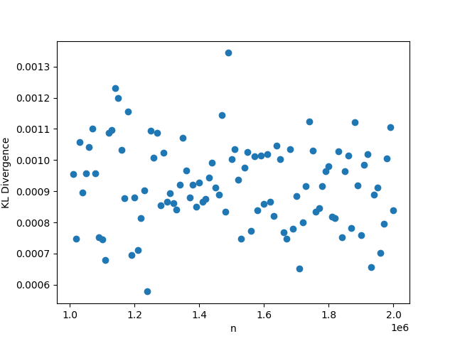
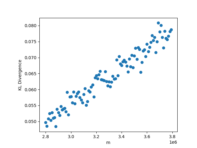
3.2
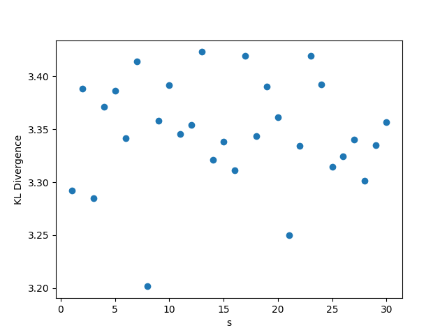
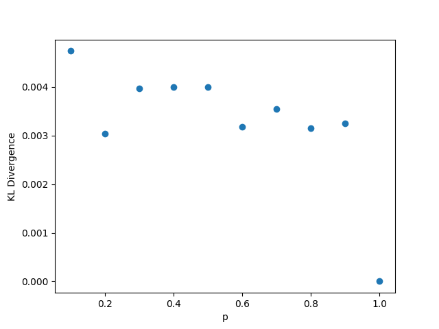
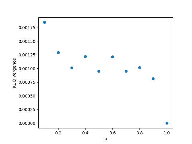
In this setting, whenever we fix , we choose the value , and . As usual, when we fix the other parameters, we choose and . The results may be seen in Figure 2. In this setting, the KL divergence is nearly zero regardless of changes in the parameters. The low value of the KL divergence indicates that the simulated and hypothetical distributions are nearly identical, reinforcing Theorem 1. We note that when grows, the distribution of will become increasingly skewed, so and may need to be larger to get the same degree of convergence in distribution. While we can see in panel (c) that the KL divergence does increase with , the value is still very small (0.012) even for for these values of and , however.

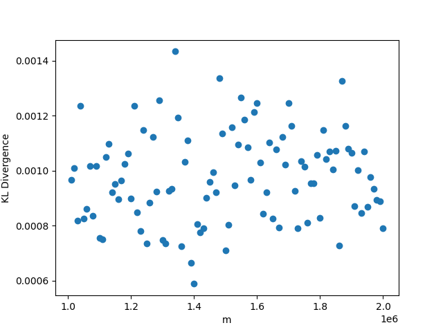
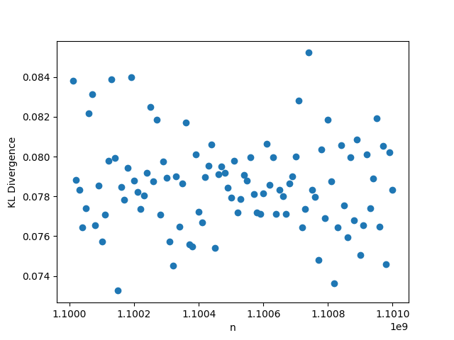
3.3
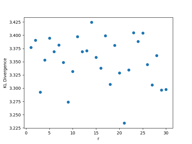
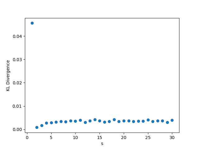
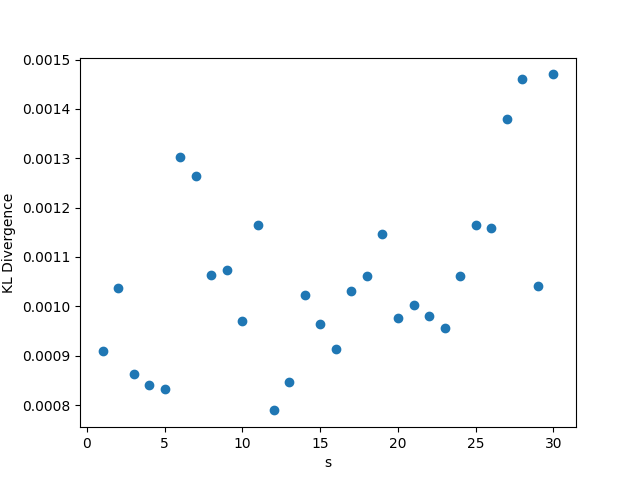
In this setting, whenever we fix , we choose the value , and . As usual, when we fix the other parameters, we choose and . The results may be seen in Figure 3. Again in this setting, the KL divergence remains nearly 0 regardless of the values of the parameters, reinforcing Theorem 1.
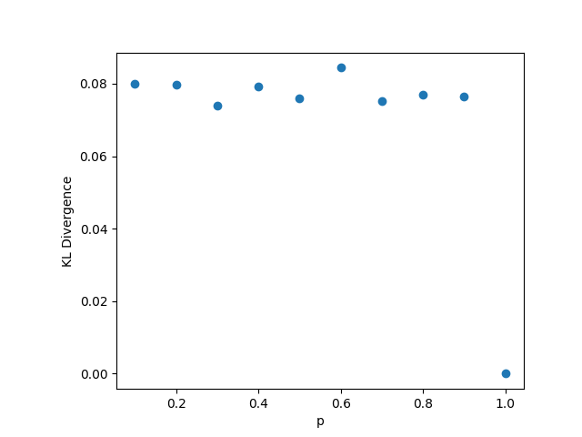
3.4
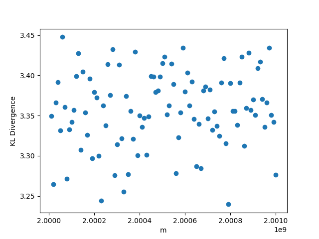
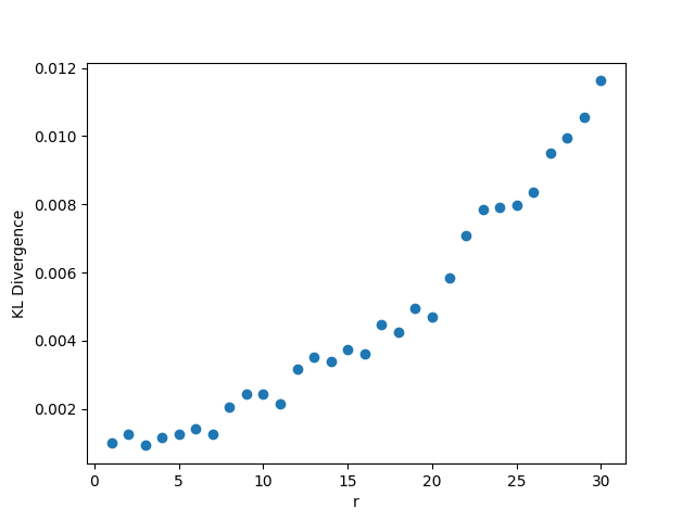
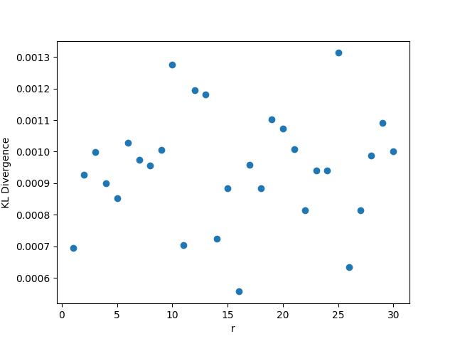
In this setting, whenever we fix , we choose the value , and . Unlike in previous cases, when the remaining parameters are fixed, we choose and , while . The results may be seen in Figure 4. The reason for the change in the default value for can be explained by considering panels (b) and (c) where and vary. We can see that the KL divergence spikes when : this comes from the fact that in this case, the hypothesized limiting distribution has 0 variance, so the Normal distribution we are comparing to collapses. Since for any finite and , the distribution of is not 0, the KL divergence is much larger at this point. Excluding this case, the KL divergences in these plots are all small, indicating close similarity between the simulated distributions and the proposed hypothetical distributions. We also note in panel (d) that increasing results in a worse KL divergence, but this also means that the ratio is increasing, meaning that we are further from the limiting regime we are considering in this case. The maximum value of the KL divergence is still quite small for this range of , however.
4 Conclusion
We studied the limiting distribution of a function of two independent Binomial random variables, in the setting where the number of trials for both variables grows large, but the rates of growth for those two quantities may differ. We were able to show that under several parameter regimes, the limiting distribution after centering and scaling is Normal, with a given variance. However, this does not exhaust the range of possible values for which one could consider this function: For example, in lubberts2025 , the authors considered the case where (for the special case of ), which is not addressed by our results here. While our results determine the appropriate values for the mean and variance of in the case when and are large, determining the behavior of higher moments would require a more careful analysis of the quadratic remainder term than the one undertaken in the present work. As a final remark, we note that even with random variables as well-studied as the Binomial, there still remain many interesting questions to explore.
References
- [1] Kai Lai Chung. A course in probability theory. Elsevier, 2000.
- [2] Roger A Horn and Charles R Johnson. Matrix analysis. Cambridge university press, 2012.
- [3] Zachary Lubberts, Avanti Athreya, Youngser Park, and Carey E Priebe. Random line graphs and edge-attributed network inference. Bernoulli, 2025. arXiv:2103.14726.