This paper was converted on www.awesomepapers.org from LaTeX by an anonymous user.
Want to know more? Visit the Converter page.

Linear Convergent Decentralized Optimization with Compression

Xiaorui Liu1, Yao Li2,3, Rongrong Wang3,2, Jiliang Tang1 & Ming Yan3,2
 1 Department of Computer Science and Engineering
 2 Department of Mathematics
 3 Department of Computational Mathematics, Science and Engineering
 Michigan State University, East Lansing, MI 48823, USA
 {xiaorui,liyao6,wongron6,tangjili,myan}@msu.edu
Abstract

Communication compression has become a key strategy to speed up distributed optimization. However, existing decentralized algorithms with compression mainly focus on compressing DGD-type algorithms. They are unsatisfactory in terms of convergence rate, stability, and the capability to handle heterogeneous data. Motivated by primal-dual algorithms, this paper proposes the first LinEAr convergent Decentralized algorithm with compression, LEAD. Our theory describes the coupled dynamics of the inexact primal and dual update as well as compression error, and we provide the first consensus error bound in such settings without assuming bounded gradients. Experiments on convex problems validate our theoretical analysis, and empirical study on deep neural nets shows that LEAD is applicable to non-convex problems.

\etocdepthtag

.tocmtchapter \etocsettagdepthmtchaptersubsection \etocsettagdepthmtappendixnone

1 Introduction

Distributed optimization solves the following optimization problem

𝒙:=argmin𝒙d[f(𝒙):=1ni=1nfi(𝒙)]\displaystyle{\bm{x}}^{*}:=\operatorname*{arg\,min}_{{\bm{x}}\in\mathbb{R}^{d}}\Big{[}f({\bm{x}}):=\frac{1}{n}\sum_{i=1}^{n}f_{i}({\bm{x}})\Big{]} (1)

with nn computing agents and a communication network. Each fi(𝒙):df_{i}({\bm{x}}):\mathbb{R}^{d}\rightarrow\mathbb{R} is a local objective function of agent ii and typically defined on the data 𝒟i\mathcal{D}_{i} settled at that agent. The data distributions {𝒟i}\{\mathcal{D}_{i}\} can be heterogeneous depending on the applications such as in federated learning. The variable 𝒙d{\bm{x}}\in\mathbb{R}^{d} often represents model parameters in machine learning. A distributed optimization algorithm seeks an optimal solution that minimizes the overall objective function f(𝒙)f({\bm{x}}) collectively. According to the communication topology, existing algorithms can be conceptually categorized into centralized and decentralized ones. Specifically, centralized algorithms require global communication between agents (through central agents or parameter servers). While decentralized algorithms only require local communication between connected agents and are more widely applicable than centralized ones. In both paradigms, the computation can be relatively fast with powerful computing devices; efficient communication is the key to improve algorithm efficiency and system scalability, especially when the network bandwidth is limited.

In recent years, various communication compression techniques, such as quantization and sparsification, have been developed to reduce communication costs. Notably, extensive studies (Seide et al., 2014; Alistarh et al., 2017; Bernstein et al., 2018; Stich et al., 2018; Karimireddy et al., 2019; Mishchenko et al., 2019; Tang et al., 2019b; Liu et al., 2020) have utilized gradient compression to significantly boost communication efficiency for centralized optimization. They enable efficient large-scale optimization while maintaining comparable convergence rates and practical performance with their non-compressed counterparts. This great success has suggested the potential and significance of communication compression in decentralized algorithms.

While extensive attention has been paid to centralized optimization, communication compression is relatively less studied in decentralized algorithms because the algorithm design and analysis are more challenging in order to cover general communication topologies. There are recent efforts trying to push this research direction. For instance, DCD-SGD and ECD-SGD (Tang et al., 2018a) introduce difference compression and extrapolation compression to reduce model compression error. (Reisizadeh et al., 2019a; b) introduce QDGD and QuanTimed-DSGD to achieve exact convergence with small stepsize. DeepSqueeze (Tang et al., 2019a) directly compresses the local model and compensates the compression error in the next iteration. CHOCO-SGD (Koloskova et al., 2019; 2020) presents a novel quantized gossip algorithm that reduces compression error by difference compression and preserves the model average. Nevertheless, most existing works focus on the compression of primal-only algorithms, i.e., reduce to DGD (Nedic & Ozdaglar, 2009; Yuan et al., 2016) or P-DSGD (Lian et al., 2017). They are unsatisfying in terms of convergence rate, stability, and the capability to handle heterogeneous data. Part of the reason is that they inherit the drawback of DGD-type algorithms, whose convergence rate is slow in heterogeneous data scenarios where the data distributions are significantly different from agent to agent.

In the literature of decentralized optimization, it has been proved that primal-dual algorithms can achieve faster converge rates and better support heterogeneous data (Ling et al., 2015; Shi et al., 2015; Li et al., 2019; Yuan et al., 2020). However, it is unknown whether communication compression is feasible for primal-dual algorithms and how fast the convergence can be with compression. In this paper, we attempt to bridge this gap by investigating the communication compression for primal-dual decentralized algorithms. Our major contributions can be summarized as:

  • We delineate two key challenges in the algorithm design for communication compression in decentralized optimization, i.e., data heterogeneity and compression error, and motivated by primal-dual algorithms, we propose a novel decentralized algorithm with compression, LEAD.

  • We prove that for LEAD, a constant stepsize in the range (0,2/(μ+L)](0,2/(\mu+L)] is sufficient to ensure linear convergence for strongly convex and smooth objective functions. To the best of our knowledge, LEAD is the first linear convergent decentralized algorithm with compression. Moreover, LEAD provably works with unbiased compression of arbitrary precision.

  • We further prove that if the stochastic gradient is used, LEAD converges linearly to the O(σ2)O(\sigma^{2}) neighborhood of the optimum with constant stepsize. LEAD is also able to achieve exact convergence to the optimum with diminishing stepsize.

  • Extensive experiments on convex problems validate our theoretical analyses, and the empirical study on training deep neural nets shows that LEAD is applicable for nonconvex problems. LEAD achieves state-of-art computation and communication efficiency in all experiments and significantly outperforms the baselines on heterogeneous data. Moreover, LEAD is robust to parameter settings and needs minor effort for parameter tuning.

2 Related Works

Decentralized optimization can be traced back to the work by Tsitsiklis et al. (1986). DGD (Nedic & Ozdaglar, 2009) is the most classical decentralized algorithm. It is intuitive and simple but converges slowly due to the diminishing stepsize that is needed to obtain the optimal solution (Yuan et al., 2016). Its stochastic version D-PSGD (Lian et al., 2017) has been shown effective for training nonconvex deep learning models. Algorithms based on primal-dual formulations or gradient tracking are proposed to eliminate the convergence bias in DGD-type algorithms and improve the convergence rate, such as D-ADMM (Mota et al., 2013), DLM (Ling et al., 2015), EXTRA (Shi et al., 2015), NIDS (Li et al., 2019), D2D^{2} (Tang et al., 2018b), Exact Diffusion (Yuan et al., 2018), OPTRA(Xu et al., 2020), DIGing (Nedic et al., 2017), GSGT (Pu & Nedić, 2020), etc.

Recently, communication compression is applied to decentralized settings by Tang et al. (2018a). It proposes two algorithms, i.e., DCD-SGD and ECD-SGD, which require compression of high accuracy and are not stable with aggressive compression. Reisizadeh et al. (2019a; b) introduce QDGD and QuanTimed-DSGD to achieve exact convergence with small stepsize and the convergence is slow. DeepSqueeze (Tang et al., 2019a) compensates the compression error to the compression in the next iteration. Motivated by the quantized average consensus algorithms, such as (Carli et al., 2010), the quantized gossip algorithm CHOCO-Gossip (Koloskova et al., 2019) converges linearly to the consensual solution. Combining CHOCO-Gossip and D-PSGD leads to a decentralized algorithm with compression, CHOCO-SGD, which converges sublinearly under the strong convexity and gradient boundedness assumptions. Its nonconvex variant is further analyzed in (Koloskova et al., 2020). A new compression scheme using the modulo operation is introduced in (Lu & De Sa, 2020) for decentralized optimization. A general algorithmic framework aiming to maintain the linear convergence of distributed optimization under compressed communication is considered in (Magnússon et al., 2020). It requires a contractive property that is not satisfied by many decentralized algorithms including the algorithm in this paper.

3 Algorithm

We first introduce notations and definitions used in this work. We use bold upper-case letters such as 𝐗{\mathbf{X}} to define matrices and bold lower-case letters such as 𝒙{\bm{x}} to define vectors. Let 𝟏{\bm{1}} and 𝟎{\bm{0}} be vectors with all ones and zeros, respectively. Their dimensions will be provided when necessary. Given two matrices 𝐗,𝐘n×d{\mathbf{X}},~{}{\mathbf{Y}}\in\mathbb{R}^{n\times d}, we define their inner product as 𝐗,𝐘=tr(𝐗𝐘)\langle{\mathbf{X}},{\mathbf{Y}}\rangle=\text{tr}({\mathbf{X}}^{\top}{\mathbf{Y}}) and the norm as 𝐗=𝐗,𝐗\|{\mathbf{X}}\|=\sqrt{\langle{\mathbf{X}},{\mathbf{X}}\rangle}. We further define 𝐗,𝐘𝐏=tr(𝐗𝐏𝐘)\langle{\mathbf{X}},{\mathbf{Y}}\rangle_{{\mathbf{P}}}=\text{tr}({\mathbf{X}}^{\top}{\mathbf{P}}{\mathbf{Y}}) and 𝐗𝐏=𝐗,𝐗𝐏\|{\mathbf{X}}\|_{{\mathbf{P}}}=\sqrt{\langle{\mathbf{X}},{\mathbf{X}}\rangle}_{{\mathbf{P}}} for any given symmetric positive semidefinite matrix 𝐏n×n{\mathbf{P}}\in\mathbb{R}^{n\times n}. For simplicity, we will majorly use the matrix notation in this work. For instance, each agent ii holds an individual estimate 𝒙id{\bm{x}}_{i}\in\mathbb{R}^{d} of the global variable 𝒙d{\bm{x}}\in\mathbb{R}^{d}. Let 𝐗k{\mathbf{X}}^{k} and 𝐅(𝐗k)\nabla{\mathbf{F}}({\mathbf{X}}^{k}) be the collections of {𝒙ik}i=1n\{{\bm{x}}_{i}^{k}\}_{i=1}^{n} and {fi(𝒙ik)}i=1n\{\nabla f_{i}({\bm{x}}_{i}^{k})\}_{i=1}^{n} which are defined below:

𝐗k=[𝒙1k,,𝒙nk]n×d,𝐅(𝐗k)=[f1(𝒙1k),,fn(𝒙nk)]n×d.\displaystyle{\mathbf{X}}^{k}=\left[{{\bm{x}}_{1}^{k}},\dots,{{\bm{x}}_{n}^{k}}\right]^{\top}\in\mathbb{R}^{n\times d},~{}~{}~{}\nabla{\mathbf{F}}({\mathbf{X}}^{k})=\left[\nabla f_{1}({\bm{x}}_{1}^{k}),\dots,\nabla f_{n}({\bm{x}}_{n}^{k})\right]^{\top}\in\mathbb{R}^{n\times d}. (2)

We use 𝐅(𝐗k;ξk)\nabla{\mathbf{F}}({\mathbf{X}}^{k};\xi^{k}) to denote the stochastic approximation of 𝐅(𝐗k)\nabla{\mathbf{F}}({\mathbf{X}}^{k}). With these notations, the update 𝐗k+1=𝐗kη𝐅(𝐗k;ξk){\mathbf{X}}^{k+1}={\mathbf{X}}^{k}-\eta\nabla{\mathbf{F}}({\mathbf{X}}^{k};\xi^{k}) means that 𝒙ik+1=𝒙ikηfi(𝒙ik;ξik){\bm{x}}_{i}^{k+1}={\bm{x}}_{i}^{k}-\eta\nabla f_{i}({\bm{x}}_{i}^{k};\xi_{i}^{k}) for all ii. In this paper, we need the average of all rows in 𝐗k{\mathbf{X}}^{k} and 𝐅(𝐗k)\nabla{\mathbf{F}}({\mathbf{X}}^{k}), so we define 𝐗¯k=(𝟏𝐗k)/n\mkern 1.5mu\overline{\mkern-1.5mu{\mathbf{X}}\mkern-1.5mu}\mkern 1.5mu^{k}=({{\bm{1}}^{\top}{\mathbf{X}}^{k}})/{n} and ¯𝐅(𝐗k)=(𝟏𝐅(𝐗k))/n\mkern 1.5mu\overline{\mkern-1.5mu\nabla\mkern-1.5mu}\mkern 1.5mu{\mathbf{F}}({\mathbf{X}}^{k})=({{\bm{1}}^{\top}\nabla{\mathbf{F}}({\mathbf{X}}^{k})})/{n}. They are row vectors, and we will take a transpose if we need a column vector. The pseudoinverse of a matrix 𝐌{\mathbf{M}} is denoted as 𝐌{\mathbf{M}}^{\dagger}. The largest, iith-largest, and smallest nonzero eigenvalues of a symmetric matrix 𝐌{\mathbf{M}} are λmax(𝐌)\lambda_{\max}({\mathbf{M}}), λi(𝐌)\lambda_{i}({\mathbf{M}}), and λmin(𝐌)\lambda_{\min}({\mathbf{M}}).

Assumption 1 (Mixing matrix).

The connected network 𝒢={𝒱,}{\mathcal{G}}=\{{\mathcal{V}},{\mathcal{E}}\} consists of a node set 𝒱={1,2,,n}{\mathcal{V}}=\{1,2,\dots,n\} and an undirected edge set {\mathcal{E}}. The primitive symmetric doubly-stochastic matrix 𝐖=[wij]n×n{\mathbf{W}}=[w_{ij}]\in\mathbb{R}^{n\times n} encodes the network structure such that wij=0w_{ij}=0 if nodes ii and jj are not connected and cannot exchange information.

Assumption 1 implies that 1<λn(𝐖)λn1(𝐖)λ2(𝐖)<λ1(𝐖)=1-1<\lambda_{n}({\mathbf{W}})\leq\lambda_{n-1}({\mathbf{W}})\leq\cdots\lambda_{2}({\mathbf{W}})<\lambda_{1}({\mathbf{W}})=1 and 𝐖𝟏=𝟏{\mathbf{W}}{\bm{1}}={\bm{1}} (Xiao & Boyd, 2004; Shi et al., 2015). The matrix multiplication 𝐗k+1=𝐖𝐗k{\mathbf{X}}^{k+1}={\mathbf{W}}{\mathbf{X}}^{k} describes that agent ii takes a weighted sum from its neighbors and itself, i.e., 𝒙ik+1=j𝒩i{i}wij𝒙jk{\bm{x}}_{i}^{k+1}=\sum_{j\in\mathcal{N}_{i}\cup\{i\}}{w}_{ij}{\bm{x}}^{k}_{j}, where 𝒩i\mathcal{N}_{i} denotes the neighbors of agent ii.

3.1 The Proposed Algorithm

The proposed algorithm LEAD to solve problem (1) is showed in Alg. 1 with matrix notations for conciseness. We will refer to the line number in the analysis. A complete algorithm description from the agent’s perspective can be found in Appendix A. The motivation behind Alg. 1 is to achieve two goals: (a) consensus (𝒙ik(𝐗¯k)𝟎{\bm{x}}_{i}^{k}-(\mkern 1.5mu\overline{\mkern-1.5mu{\mathbf{X}}\mkern-1.5mu}\mkern 1.5mu^{k})^{\top}\rightarrow{\bm{0}}) and (b) convergence ((𝐗¯k)𝒙(\mkern 1.5mu\overline{\mkern-1.5mu{\mathbf{X}}\mkern-1.5mu}\mkern 1.5mu^{k})^{\top}\rightarrow{\bm{x}}^{*}). We first discuss how goal (a) leads to goal (b) and then explain how LEAD fulfills goal (a).

Algorithm 1 LEAD

Input: Stepsize η\eta, parameter (α,γ\alpha,~{}\gamma), 𝐗0,𝐇1,𝐃1=(𝐈𝐖)𝐙{\mathbf{X}}^{0},~{}{\mathbf{H}}^{1},~{}{\mathbf{D}}^{1}=({\mathbf{I}}-{\mathbf{W}}){\mathbf{Z}} for any 𝐙{\mathbf{Z}}
Output: 𝐗K{\mathbf{X}}^{K} or 1/ni=1n𝐗iK1/n\sum_{i=1}^{n}{\mathbf{X}}^{K}_{i}

1:𝐇w1=𝐖𝐇1{\mathbf{H}}_{w}^{1}={\mathbf{W}}{\mathbf{H}}^{1}
2:𝐗1=𝐗0η𝐅(𝐗0;ξ0){\mathbf{X}}^{1}={\mathbf{X}}^{0}-\eta\nabla{\mathbf{F}}({\mathbf{X}}^{0};\xi^{0})
3:for k=1,2,,K1k=1,2,\cdots,K-1 do
4:     𝐘k=𝐗kη𝐅(𝐗k;ξk)η𝐃k{\mathbf{Y}}^{k}={\mathbf{X}}^{k}-\eta\nabla{\mathbf{F}}({\mathbf{X}}^{k};\xi^{k})-\eta{\mathbf{D}}^{k}
5:     𝐘^k,𝐘^wk,𝐇k+1,𝐇wk+1\hat{\mathbf{Y}}^{k},\hat{\mathbf{Y}}^{k}_{w},{\mathbf{H}}^{k+1},{\mathbf{H}}_{w}^{k+1} = Comm(𝐘k,𝐇k,𝐇wk{\mathbf{Y}}^{k},{\mathbf{H}}^{k},{\mathbf{H}}_{w}^{k})
6:     𝐃k+1=𝐃k+γ2η(𝐘^k𝐘^wk){\mathbf{D}}^{k+1}={\mathbf{D}}^{k}+\frac{\gamma}{2\eta}(\hat{\mathbf{Y}}^{k}-\hat{\mathbf{Y}}^{k}_{w})
7:     𝐗k+1=𝐗kη𝐅(𝐗k;ξk)η𝐃k+1{\mathbf{X}}^{k+1}={\mathbf{X}}^{k}-\eta\nabla{\mathbf{F}}({\mathbf{X}}^{k};\xi^{k})-\eta{\mathbf{D}}^{k+1}
8:end for
9:procedure Comm(𝐘,𝐇,𝐇w{\mathbf{Y}},{\mathbf{H}},{\mathbf{H}}_{w})
10:     𝐐={\mathbf{Q}}= Compress(𝐘𝐇{\mathbf{Y}}-{\mathbf{H}})
11:     𝐘^=𝐇+𝐐\hat{\mathbf{Y}}={\mathbf{H}}+{\mathbf{Q}}
12:     𝐘^w=𝐇w+𝐖𝐐\hat{\mathbf{Y}}_{w}={\mathbf{H}}_{w}+{\mathbf{W}}{\mathbf{Q}}
13:     𝐇=(1α)𝐇+α𝐘^{\mathbf{H}}=(1-\alpha){\mathbf{H}}+\alpha\hat{\mathbf{Y}}
14:     𝐇w=(1α)𝐇w+α𝐘^w{\mathbf{H}}_{w}=(1-\alpha){\mathbf{H}}_{w}+\alpha\hat{\mathbf{Y}}_{w}
15:     Return: 𝐘^,𝐘^w,𝐇,𝐇w\hat{\mathbf{Y}},\hat{\mathbf{Y}}_{w},{\mathbf{H}},{\mathbf{H}}_{w}
16:end procedure

In essence, LEAD runs the approximate SGD globally and reduces to the exact SGD under consensus. One key property for LEAD is 𝟏n×1𝐃k=𝟎{\bm{1}}_{n\times 1}^{\top}{\mathbf{D}}^{k}={\bm{0}}, regardless of the compression error in 𝐘^k\hat{\mathbf{Y}}^{k}. It holds because that for the initialization, we require 𝐃1=(𝐈𝐖)𝐙{\mathbf{D}}^{1}=({\mathbf{I}}-{\mathbf{W}}){\mathbf{Z}} for some 𝐙n×d{\mathbf{Z}}\in\mathbb{R}^{n\times d}, e.g., 𝐃1=𝟎n×d{\mathbf{D}}^{1}={\bm{0}}^{n\times d}, and that the update of 𝐃k{\mathbf{D}}^{k} ensures 𝐃k𝐑𝐚𝐧𝐠𝐞(𝐈𝐖){\mathbf{D}}^{k}\in\mathbf{Range}({\mathbf{I}}-{\mathbf{W}}) for all kk and 𝟏n×1(𝐈𝐖)=𝟎{\bm{1}}_{n\times 1}^{\top}({\mathbf{I}}-{\mathbf{W}})={\bm{0}} as we will explain later. Therefore, multiplying (1/n)𝟏n×1(1/n){{\bm{1}}_{n\times 1}^{\top}} on both sides of Line 7 leads to a global average view of Alg. 1:

𝐗¯k+1=𝐗¯kη¯𝐅(𝐗k;ξk),\displaystyle\mkern 1.5mu\overline{\mkern-1.5mu{\mathbf{X}}\mkern-1.5mu}\mkern 1.5mu^{k+1}=\mkern 1.5mu\overline{\mkern-1.5mu{\mathbf{X}}\mkern-1.5mu}\mkern 1.5mu^{k}-\eta\mkern 1.5mu\overline{\mkern-1.5mu\nabla\mkern-1.5mu}\mkern 1.5mu{\mathbf{F}}({\mathbf{X}}^{k};\xi^{k}), (3)

which doesn’t contain the compression error. Note that this is an approximate SGD step because, as shown in (2), the gradient 𝐅(𝐗k;ξk)\nabla{\mathbf{F}}({\mathbf{X}}^{k};\xi^{k}) is not evaluated on a global synchronized model 𝐗¯k\mkern 1.5mu\overline{\mkern-1.5mu{\mathbf{X}}\mkern-1.5mu}\mkern 1.5mu^{k}. However, if the solution converges to the consensus solution, i.e., 𝒙ik(𝐗¯k)𝟎{\bm{x}}_{i}^{k}-(\mkern 1.5mu\overline{\mkern-1.5mu{\mathbf{X}}\mkern-1.5mu}\mkern 1.5mu^{k})^{\top}\rightarrow{\bm{0}}, then 𝔼ξk[¯𝐅(𝐗k;ξk)f(𝐗¯k;ξk)]𝟎{\mathbb{E}}_{\xi^{k}}[\mkern 1.5mu\overline{\mkern-1.5mu\nabla\mkern-1.5mu}\mkern 1.5mu{\mathbf{F}}({\mathbf{X}}^{k};\xi^{k})-{\nabla}f(\mkern 1.5mu\overline{\mkern-1.5mu{\mathbf{X}}\mkern-1.5mu}\mkern 1.5mu^{k};\xi^{k})]\rightarrow{\bm{0}} and (3) gradually reduces to exact SGD.

With the establishment of how consensus leads to convergence, the obstacle becomes how to achieve consensus under local communication and compression challenges. It requires addressing two issues, i.e., data heterogeneity and compression error. To deal with these issues, existing algorithms, such as DCD-SGD, ECD-SGD, QDGD, DeepSqueeze, Moniqua, and CHOCO-SGD, need a diminishing or constant but small stepsize depending on the total number of iterations. However, these choices unavoidably cause slower convergence and bring in the difficulty of parameter tuning. In contrast, LEAD takes a different way to solve these issues, as explained below.

Data heterogeneity. It is common in distributed settings that there exists data heterogeneity among agents, especially in real-world applications where different agents collect data from different scenarios. In other words, we generally have fi(𝒙)fj(𝒙)f_{i}({\bm{x}})\neq f_{j}({\bm{x}}) for iji\neq j. The optimality condition of problem (1) gives 𝟏n×1𝐅(𝐗)=𝟎{\bm{1}}_{n\times 1}^{\top}\nabla{\mathbf{F}}({\mathbf{X}}^{*})={\bm{0}}, where 𝐗=[𝒙,,𝒙]{\mathbf{X}}^{*}=[{\bm{x}}^{*},\cdots,{\bm{x}}^{*}] is a consensual and optimal solution. The data heterogeneity and optimality condition imply that there exist at least two agents ii and jj such that fi(𝒙)𝟎\nabla f_{i}({\bm{x}}^{*})\neq{\bm{0}} and fj(𝒙)𝟎\nabla f_{j}({\bm{x}}^{*})\neq{\bm{0}}. As a result, a simple D-PSGD algorithm cannot converge to the consensual and optimal solution as 𝐗𝐖𝐗η𝔼ξ𝐅(𝐗;ξ){\mathbf{X}}^{*}\neq{\mathbf{W}}{\mathbf{X}}^{*}-\eta{\mathbb{E}}_{\xi}\nabla{\mathbf{F}}({\mathbf{X}}^{*};\xi) even when the stochastic gradient variance is zero.

Gradient correction. Primal-dual algorithms or gradient tracking algorithms are able to convergence much faster than DGD-type algorithms by handling the data heterogeneity issue, as introduced in Section 2. Specifically, LEAD is motivated by the design of primal-dual algorithm NIDS (Li et al., 2019) and the relation becomes clear if we consider the two-step reformulation of NIDS adopted in (Li & Yan, 2019):

𝐃k+1\displaystyle{\mathbf{D}}^{k+1} =𝐃k+𝐈𝐖2η(𝐗kη𝐅(𝐗k)η𝐃k),\displaystyle={\mathbf{D}}^{k}+\frac{{\mathbf{I}}-{\mathbf{W}}}{2\eta}({\mathbf{X}}^{k}-\eta\nabla{\mathbf{F}}({\mathbf{X}}^{k})-\eta{\mathbf{D}}^{k}), (4)
𝐗k+1\displaystyle{\mathbf{X}}^{k+1} =𝐗kη𝐅(𝐗k)η𝐃k+1,\displaystyle={\mathbf{X}}^{k}-\eta\nabla{\mathbf{F}}({\mathbf{X}}^{k})-\eta{\mathbf{D}}^{k+1}, (5)

where 𝐗k{\mathbf{X}}^{k} and 𝐃k{\mathbf{D}}^{k} represent the primal and dual variables respectively. The dual variable 𝐃k{\mathbf{D}}^{k} plays the role of gradient correction. As kk\rightarrow\infty, we expect 𝐃k𝐅(𝐗){\mathbf{D}}^{k}\rightarrow-\nabla{\mathbf{F}}({\mathbf{X}}^{*}) and 𝐗k{\mathbf{X}}^{k} will converge to 𝐗{\mathbf{X}}^{*} via the update in (5) since 𝐃k+1{\mathbf{D}}^{k+1} corrects the nonzero gradient 𝐅(𝐗k)\nabla{\mathbf{F}}({\mathbf{X}}^{k}) asymptotically. The key design of Alg. 1 is to provide compression for the auxiliary variable defined as 𝐘k=𝐗kη𝐅(𝐗k)η𝐃k{\mathbf{Y}}^{k}={\mathbf{X}}^{k}-\eta\nabla{\mathbf{F}}({\mathbf{X}}^{k})-\eta{\mathbf{D}}^{k}. Such design ensures that the dual variable 𝐃k{\mathbf{D}}^{k} lies in Range(𝐈𝐖)\textbf{Range}({\mathbf{I}}-{\mathbf{W}}), which is essential for convergence. Moreover, it achieves the implicit error compression as we will explain later. To stabilize the algorithm with inexact dual update, we introduce a parameter γ\gamma to control the stepsize in the dual update. Therefore, if we ignore the details of the compression, Alg. 1 can be concisely written as

𝐘k\displaystyle{\mathbf{Y}}^{k} =𝐗kη𝐅(𝐗k;ξk)η𝐃k\displaystyle={\mathbf{X}}^{k}-\eta\nabla{\mathbf{F}}({\mathbf{X}}^{k};\xi^{k})-\eta{\mathbf{D}}^{k} (6)
𝐃k+1\displaystyle{\mathbf{D}}^{k+1} =𝐃k+γ2η(𝐈𝐖)𝐘^k\displaystyle={\mathbf{D}}^{k}+\frac{\gamma}{2\eta}({\mathbf{I}}-{\mathbf{W}})\hat{\mathbf{Y}}^{k} (7)
𝐗k+1\displaystyle{\mathbf{X}}^{k+1} =𝐗kη𝐅(𝐗k;ξk)η𝐃k+1\displaystyle={\mathbf{X}}^{k}-\eta\nabla{\mathbf{F}}({\mathbf{X}}^{k};\xi^{k})-\eta{\mathbf{D}}^{k+1} (8)

where 𝐘^k\hat{\mathbf{Y}}^{k} represents the compression of 𝐘k{\mathbf{Y}}^{k} and 𝐅(𝐗k;ξk){\mathbf{F}}({\mathbf{X}}^{k};\xi^{k}) denote the stochastic gradients.

Nevertheless, how to compress the communication and how fast the convergence we can attain with compression error are unknown. In the following, we propose to carefully control the compression error by difference compression and error compensation such that the inexact dual update (Line 6) and primal update (Line 7) can still guarantee the convergence as proved in Section 4.

Compression error. Different from existing works, which typically compress the primal variable 𝐗k{\mathbf{X}}^{k} or its difference, LEAD first construct an intermediate variable 𝐘k{\mathbf{Y}}^{k} and apply compression to obtain its coarse representation 𝐘^k\hat{\mathbf{Y}}^{k} as shown in the procedure Comm(𝐘,𝐇,𝐇w)\textsc{Comm}({\mathbf{Y}},{\mathbf{H}},{\mathbf{H}}_{w}):

  • Compress the difference between 𝐘{\mathbf{Y}} and the state variable 𝐇{\mathbf{H}} as 𝐐{\mathbf{Q}};

  • 𝐐{\mathbf{Q}} is encoded into the low-bit representation, which enables the efficient local communication step 𝐘^w=𝐇w+𝐖𝐐\hat{\mathbf{Y}}_{w}={\mathbf{H}}_{w}+{\mathbf{W}}{\mathbf{Q}}. It is the only communication step in each iteration.

  • Each agent recovers its estimate 𝐘^\hat{\mathbf{Y}} by 𝐘^=𝐇+𝐐\hat{\mathbf{Y}}={\mathbf{H}}+{\mathbf{Q}} and we have 𝐘^w=𝐖𝐘^\hat{\mathbf{Y}}_{w}={\mathbf{W}}\hat{\mathbf{Y}}.

  • States 𝐇{\mathbf{H}} and 𝐇w{\mathbf{H}}_{w} are updated based on 𝐘^\hat{\mathbf{Y}} and 𝐘^w\hat{\mathbf{Y}}_{w}, respectively. We have 𝐇w=𝐖𝐇{\mathbf{H}}_{w}={\mathbf{W}}{\mathbf{H}}.

By this procedure, we expect when both 𝐘k{\mathbf{Y}}^{k} and 𝐇k{\mathbf{H}}^{k} converge to 𝐗{\mathbf{X}}^{*}, the compression error vanishes asymptotically due to the assumption we make for the compression operator in Assumption 2.

Remark 1.

Note that difference compression is also applied in DCD-PSGD (Tang et al., 2018a) and CHOCO-SGD (Koloskova et al., 2019), but their state update is the simple integration of the compressed difference. We find this update is usually too aggressive and cause instability as showed in our experiments. Therefore, we adopt a momentum update 𝐇=(1α)𝐇+α𝐘^{\mathbf{H}}=(1-\alpha){\mathbf{H}}+\alpha\hat{\mathbf{Y}} motivated from DIANA (Mishchenko et al., 2019), which reduces the compression error for gradient compression in centralized optimization.

Implicit error compensation. On the other hand, even if the compression error exists, LEAD essentially compensates for the error in the inexact dual update (Line 6), making the algorithm more stable and robust. To illustrate how it works, let 𝐄k=𝐘^k𝐘k{\mathbf{E}}^{k}=\hat{\mathbf{Y}}^{k}-{\mathbf{Y}}^{k} denote the compression error and 𝒆ik{\bm{e}}^{k}_{i} be its ii-th row. The update of 𝐃k{\mathbf{D}}^{k} gives

𝐃k+1\displaystyle{\mathbf{D}}^{k+1} =𝐃k+γ2η(𝐘^k𝐘^wk)=𝐃k+γ2η(𝐈𝐖)𝐘k+γ2η(𝐄k𝐖𝐄k)\displaystyle={\mathbf{D}}^{k}+\frac{\gamma}{2\eta}(\hat{\mathbf{Y}}^{k}-\hat{\mathbf{Y}}^{k}_{w})={\mathbf{D}}^{k}+\frac{\gamma}{2\eta}({\mathbf{I}}-{\mathbf{W}}){\mathbf{Y}}^{k}+\frac{\gamma}{2\eta}({\mathbf{E}}^{k}-{\mathbf{W}}{\mathbf{E}}^{k})

where 𝐖𝐄k-{\mathbf{W}}{\mathbf{E}}^{k} indicates that agent ii spreads total compression error j𝒩i{i}wji𝒆ik=𝒆ik-\sum_{j\in\mathcal{N}_{i}\cup\{i\}}w_{ji}{\bm{e}}^{k}_{i}=-{\bm{e}}^{k}_{i} to all agents and 𝐄k{\mathbf{E}}^{k} indicates that each agent compensates this error locally by adding 𝒆ik{\bm{e}}^{k}_{i} back. This error compensation also explains why the global view in (3) doesn’t involve compression error.

Remark 2.

Note that in LEAD, the compression error is compensated into the model 𝐗k+1{\mathbf{X}}^{k+1} through Line 6 and Line 7 such that the gradient computation in the next iteration is aware of the compression error. This has some subtle but important difference from the error compensation or error feedback in (Seide et al., 2014; Wu et al., 2018; Stich et al., 2018; Karimireddy et al., 2019; Tang et al., 2019b; Liu et al., 2020; Tang et al., 2019a), where the error is stored in the memory and only compensated after gradient computation and before the compression.

Remark 3.

The proposed algorithm, LEAD in Alg. 1, recovers NIDS (Li et al., 2019), D2 (Tang et al., 2018b), Exact Diffusion (Yuan et al., 2018). These connections are established in Appendix B.

4 Theoretical Analysis

In this section, we show the convergence rate for the proposed algorithm LEAD. Before showing the main theorem, we make some assumptions, which are commonly used for the analysis of decentralized optimization algorithms. All proofs are provided in Appendix E.

Assumption 2 (Unbiased and CC-contracted operator).

The compression operator Q:ddQ:\mathbb{R}^{d}\rightarrow\mathbb{R}^{d} is unbiased, i.e., 𝔼Q(𝐱)=𝐱{\mathbb{E}}Q({\bm{x}})={\bm{x}}, and there exists C0C\geq 0 such that 𝔼𝐱Q(𝐱)22C𝐱22{\mathbb{E}}\|{\bm{x}}-Q({\bm{x}})\|_{2}^{2}\leq C\|{\bm{x}}\|^{2}_{2} for all 𝐱d{\bm{x}}\in\mathbb{R}^{d}.

Assumption 3 (Stochastic gradient).

The stochastic gradient fi(𝐱;ξ)\nabla f_{i}({\bm{x}};\xi) is unbiased, i.e., 𝔼ξfi(𝐱;ξ)=fi(𝐱){\mathbb{E}}_{\xi}\nabla f_{i}({\bm{x}};\xi)=\nabla f_{i}({\bm{x}}), and the stochastic gradient variance is bounded: 𝔼ξfi(𝐱;ξ)fi(𝐱)22σi2{\mathbb{E}}_{\xi}\|\nabla f_{i}({\bm{x}};\xi)-\nabla f_{i}({\bm{x}})\|_{2}^{2}\leq\sigma_{i}^{2} for all i[n]i\in[n]. Denote σ2=1ni=1nσi2.\sigma^{2}=\frac{1}{n}\sum_{i=1}^{n}\sigma_{i}^{2}.

Assumption 4.

Each fif_{i} is LL-smooth and μ\mu-strongly convex with Lμ>0L\geq\mu>0, i.e., for i=1,2,,ni=1,2,\dots,n and 𝐱,𝐲d\forall{\bm{x}},{\bm{y}}\in\mathbb{R}^{d}, we have

fi(𝒚)+fi(𝒚),𝒙𝒚+μ2𝒙𝒚2fi(𝒙)\displaystyle f_{i}({\bm{y}})+\langle\nabla f_{i}({\bm{y}}),{\bm{x}}-{\bm{y}}\rangle+\frac{\mu}{2}\|{\bm{x}}-{\bm{y}}\|^{2}\leq f_{i}({\bm{x}}) fi(𝒚)+fi(𝒚),𝒙𝒚+L2𝒙𝒚2.\displaystyle\leq f_{i}({\bm{y}})+\langle\nabla f_{i}({\bm{y}}),{\bm{x}}-{\bm{y}}\rangle+\frac{L}{2}\|{\bm{x}}-{\bm{y}}\|^{2}.
Theorem 1 (Constant stepsize).

Let {𝐗k,𝐇k,𝐃k}\{{\mathbf{X}}^{k},{\mathbf{H}}^{k},{\mathbf{D}}^{k}\} be the sequence generated from Alg. 1 and 𝐗{\mathbf{X}}^{*} is the optimal solution with 𝐃=𝐅(𝐗){\mathbf{D}}^{*}=-\nabla{\mathbf{F}}({\mathbf{X}}^{*}). Under Assumptions 1-4, for any constant stepsize η(0,2/(μ+L)]\eta\in(0,{2}/({\mu+L})], if the compression parameters α\alpha and γ\gamma satisfy

γ\displaystyle\gamma (0,min{2(3C+1)β,2μη(2μη)[2μη(2μη)]Cβ}),\displaystyle\in\left(0,\min\Big{\{}\frac{2}{(3C+1)\beta},\frac{2\mu\eta(2-\mu\eta)}{[2-\mu\eta(2-\mu\eta)]C\beta}\Big{\}}\right), (9)
α\displaystyle\alpha [Cβγ2(1+C),1a1min{2βγ4βγ,μη(2μη)}],\displaystyle\in\left[\frac{C\beta\gamma}{2(1+C)},\frac{1}{a_{1}}\min\Big{\{}\frac{2-\beta\gamma}{4-\beta\gamma},\mu\eta(2-\mu\eta)\Big{\}}\right], (10)

with βλmax(𝐈𝐖)\beta\coloneqq\lambda_{\max}({\mathbf{I}}-{\mathbf{W}}). Then, in total expectation we have

1n𝔼k+1ρ1n𝔼k+η2σ2,\displaystyle\frac{1}{n}{\mathbb{E}}\mathcal{L}^{k+1}\leq\rho\frac{1}{n}{\mathbb{E}}\mathcal{L}^{k}+\eta^{2}\sigma^{2}, (11)

where

k\displaystyle\mathcal{L}^{k} (1a1α)𝐗k𝐗2+(2η2/γ)𝔼𝐃k𝐃(𝐈𝐖)2+a1𝐇k𝐗2,\displaystyle\coloneqq(1-a_{1}\alpha)\|{\mathbf{X}}^{k}-{\mathbf{X}}^{*}\|^{2}+(2\eta^{2}/\gamma){\mathbb{E}}\|{\mathbf{D}}^{k}-{\mathbf{D}}^{*}\|^{2}_{({\mathbf{I}}-{\mathbf{W}})^{\dagger}}+a_{1}\|{\mathbf{H}}^{k}-{\mathbf{X}}^{*}\|^{2},
ρ\displaystyle\rho max{1μη(2μη)1a1α,1γ2λmax((𝐈𝐖)),1α}<1,a14(1+C)Cβγ+2\displaystyle\coloneqq\max\left\{\frac{1-\mu\eta(2-\mu\eta)}{1-a_{1}\alpha},1-{\gamma\over 2\lambda_{\max}(({\mathbf{I}}-{\mathbf{W}})^{\dagger})},~{}~{}1-\alpha\right\}<1,a_{1}\coloneqq\frac{4(1+C)}{C\beta\gamma+2}

The result holds for C0C\rightarrow 0.

Corollary 1 (Complexity bounds).

Define the condition numbers of the objective function and communication graph as κf=Lμ\kappa_{f}=\frac{L}{\mu} and κg=λmax(𝐈𝐖)λmin+(𝐈𝐖)\kappa_{g}=\frac{\lambda_{\max}({\mathbf{I}}-{\mathbf{W}})}{\lambda_{\min}^{+}({\mathbf{I}}-{\mathbf{W}})}, respectively. Under the same setting in Theorem 1, we can choose η=1L,γ=min{1Cβκf,1(1+3C)β}\eta=\frac{1}{L},\gamma=\min\{\frac{1}{C\beta\kappa_{f}},\frac{1}{(1+3C)\beta}\}, and α=𝒪(1(1+C)κf)\alpha=\mathcal{O}(\frac{1}{(1+C)\kappa_{f}}) such that

ρ=max{1𝒪(1(1+C)κf),1𝒪(1(1+C)κg),1𝒪(1Cκfκg)}.\rho=\max\left\{1-\mathcal{O}\Big{(}\frac{1}{(1+C)\kappa_{f}}\Big{)},1-\mathcal{O}\Big{(}\frac{1}{(1+C)\kappa_{g}}\Big{)},1-\mathcal{O}\Big{(}\frac{1}{C\kappa_{f}\kappa_{g}}\Big{)}\right\}.

With full-gradient (i.e., σ=0\sigma=0), we obtain the following complexity bounds:

  • LEAD converges to the ϵ\epsilon-accurate solution with the iteration complexity

    𝒪(((1+C)(κf+κg)+Cκfκg)log1ϵ).\mathcal{O}\Big{(}\big{(}(1+C)(\kappa_{f}+\kappa_{g})+C\kappa_{f}\kappa_{g}\big{)}\log\frac{1}{\epsilon}\Big{)}.
  • When C=0C=0 (i.e., there is no compression), we obtain ρ=max{1𝒪(1κf),1𝒪(1κg)},\rho=\max\{1-\mathcal{O}(\frac{1}{\kappa_{f}}),1-\mathcal{O}(\frac{1}{\kappa_{g}})\}, and the iteration complexity 𝒪((κf+κg)log1ϵ)\mathcal{O}\Big{(}(\kappa_{f}+\kappa_{g})\log\frac{1}{\epsilon}\Big{)}. This exactly recovers the convergence rate of NIDS (Li et al., 2019).

  • When Cκf+κgκfκg+κf+κg,C\leq\frac{\kappa_{f}+\kappa_{g}}{\kappa_{f}\kappa_{g}+\kappa_{f}+\kappa_{g}}, the asymptotical complexity is 𝒪((κf+κg)log1ϵ)\mathcal{O}\Big{(}(\kappa_{f}+\kappa_{g})\log\frac{1}{\epsilon}\Big{)}, which also recovers that of NIDS (Li et al., 2019) and indicates that the compression doesn’t harm the convergence in this case.

  • With C=0C=0 (or Cκf+κgκfκg+κf+κgC\leq\frac{\kappa_{f}+\kappa_{g}}{\kappa_{f}\kappa_{g}+\kappa_{f}+\kappa_{g}}) and fully connected communication graph (i.e., 𝐖=𝟏𝟏n{\mathbf{W}}=\frac{{\bm{1}}{\bm{1}}^{\top}}{n}), we have β=1\beta=1 and κg=1\kappa_{g}=1. Therefore, we obtain ρ=1𝒪(1κf)\rho=1-\mathcal{O}(\frac{1}{\kappa_{f}}) and the complexity bound 𝒪(κflog1ϵ)\mathcal{O}(\kappa_{f}log\frac{1}{\epsilon}). This recovers the convergence rate of gradient descent (Nesterov, 2013).

Remark 4.

Under the setting in Theorem 1, LEAD converges linearly to the 𝒪(σ2)\mathcal{O}(\sigma^{2}) neighborhood of the optimum and converges linearly exactly to the optimum if full gradient is used, e.g., σ=0\sigma=0. The linear convergence of LEAD holds when η<2/L\eta<2/L, but we omit the proof.

Remark 5 (Arbitrary compression precision).

Pick any η(0,2/(μ+L)],\eta\in(0,{2}/({\mu+L})], based on the compression-related constant CC and the network-related constant β\beta, we can select γ\gamma and α\alpha in certain ranges to achieve the convergence. It suggests that LEAD supports unbiased compression with arbitrary precision, i.e., any C>0C>0.

Corollary 2 (Consensus error).

Under the same setting in Theorem 1 , let 𝐱¯k=1ni=1n𝐱ik\mkern 1.5mu\overline{\mkern-1.5mu{\bm{x}}\mkern-1.5mu}\mkern 1.5mu^{k}=\frac{1}{n}\sum_{i=1}^{n}{\bm{x}}^{k}_{i} be the averaged model and 𝐇0=𝐇1{\mathbf{H}}^{0}={\mathbf{H}}^{1}, then all agents achieve consensus at the rate

1ni=1n𝔼𝒙ik𝒙¯k220nρk+2σ21ρη2.\displaystyle\frac{1}{n}\sum_{i=1}^{n}{\mathbb{E}}\left\|{\bm{x}}_{i}^{k}-\mkern 1.5mu\overline{\mkern-1.5mu{\bm{x}}\mkern-1.5mu}\mkern 1.5mu^{k}\right\|^{2}\leq\frac{2\mathcal{L}^{0}}{n}\rho^{k}+\frac{2\sigma^{2}}{1-\rho}\eta^{2}. (12)

where ρ\rho is defined as in Corollary 1 with appropriate parameter settings.

Theorem 2 (Diminishing stepsize).

Let {𝐗k,𝐇k,𝐃k}\{{\mathbf{X}}^{k},{\mathbf{H}}^{k},{\mathbf{D}}^{k}\} be the sequence generated from Alg. 1 and 𝐗{\mathbf{X}}^{*} is the optimal solution with 𝐃=𝐅(𝐗){\mathbf{D}}^{*}=-\nabla{\mathbf{F}}({\mathbf{X}}^{*}). Under Assumptions 1-4, if ηk=2θ5θ3θ4θ5k+2\eta_{k}=\frac{2\theta_{5}}{\theta_{3}\theta_{4}\theta_{5}k+2} and γk=θ4ηk\gamma_{k}=\theta_{4}\eta_{k}, by taking αk=Cβγk2(1+C)\alpha_{k}=\frac{C\beta\gamma_{k}}{2(1+C)}, in total expectation we have

1ni=1n𝔼𝒙ik𝒙2𝒪(1k)\displaystyle\frac{1}{n}\sum_{i=1}^{n}{\mathbb{E}}\left\|{\bm{x}}_{i}^{k}-{\bm{x}}^{*}\right\|^{2}\lesssim\mathcal{O}\left(\frac{1}{k}\right) (13)

where θ1,θ2,θ3,θ4\theta_{1},\theta_{2},\theta_{3},\theta_{4} and θ5\theta_{5} are constants defined in the proof. The complexity bound for arriving at the ϵ\epsilon-accurate solution is 𝒪(1ϵ)\mathcal{O}(\frac{1}{\epsilon}).

Remark 6.

Compared with CHOCO-SGD, LEAD requires unbiased compression and the convergence under biased compression is not investigated yet. The analysis of CHOCO-SGD relies on the bounded gradient assumptions, i.e., fi(𝐱)2G\|\nabla f_{i}({\bm{x}})\|^{2}\leq G, which is restrictive because it conflicts with the strong convexity while LEAD doesn’t need this assumption. Moreover, in the theorem of CHOCO-SGD, it requires a specific point set of γ\gamma while LEAD only requires γ\gamma to be within a rather large range. This may explain the advantages of LEAD over CHOCO-SGD in terms of robustness to parameter setting.

5 Numerical Experiment

We consider three machine learning problems – 2\ell_{2}-regularized linear regression, logistic regression, and deep neural network. The proposed LEAD is compared with QDGD (Reisizadeh et al., 2019a), DeepSqueeze (Tang et al., 2019a), CHOCO-SGD (Koloskova et al., 2019), and two non-compressed algorithms DGD (Yuan et al., 2016) and NIDS (Li et al., 2019).

Setup. We consider eight machines connected in a ring topology network. Each agent can only exchange information with its two 1-hop neighbors. The mixing weight is simply set as 1/31/3. For compression, we use the unbiased bb-bits quantization method with \infty-norm

Q(𝒙):=(𝒙2(b1)sign(𝒙))2(b1)|𝒙|𝒙+𝒖,\displaystyle Q_{\infty}({\bm{x}}):=\left(\|{\bm{x}}\|_{\infty}2^{-(b-1)}\operatorname{sign}({\bm{x}})\right)\cdot\left\lfloor{\frac{2^{(b-1)}|{\bm{x}}|}{\|{\bm{x}}\|_{\infty}}+{\bm{u}}}\right\rfloor, (14)

where \cdot is the Hadamard product, |𝒙||{\bm{x}}| is the elementwise absolute value of 𝒙{\bm{x}}, and 𝒖{\bm{u}} is a random vector uniformly distributed in [0,1]d[0,1]^{d}. Only sign(𝒙)({\bm{x}}), norm 𝒙\|{\bm{x}}\|_{\infty}, and integers in the bracket need to be transmitted. Note that this quantization method is similar to the quantization used in QSGD (Alistarh et al., 2017) and CHOCO-SGD (Koloskova et al., 2019), but we use the \infty-norm scaling instead of the 22-norm. This small change brings significant improvement on compression precision as justified both theoretically and empirically in Appendix C. In this section, we choose 22-bit quantization and quantize the data blockwise (block size = 512512).

For all experiments, we tune the stepsize η\eta from {0.01,0.05,0.1,0.5}\{0.01,0.05,0.1,0.5\}. For QDGD, CHOCO-SGD and Deepsqueeze, γ\gamma is tuned from {0.01,0.1,0.2,0.4,0.6,0.8,1.0}\{0.01,0.1,0.2,0.4,0.6,0.8,1.0\}. Note that different notations are used in their original papers. Here we uniformly denote the stepsize as η\eta and the additional parameter in these algorithms as γ\gamma for simplicity. For LEAD, we simply fix α=0.5\alpha=0.5 and γ=1.0\gamma=1.0 for all experiments since we find LEAD is robust to parameter settings as we validate in the parameter sensitivity analysis in Appendix D.1. This indicates the minor effort needed for tuning LEAD. Detailed parameter settings for all experiments are summarized in Appendix D.3.

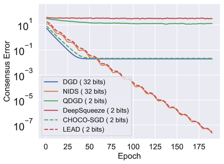
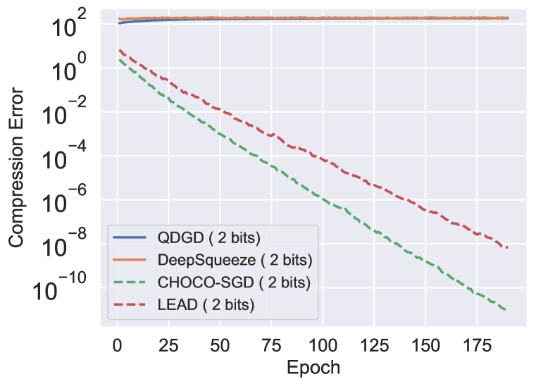
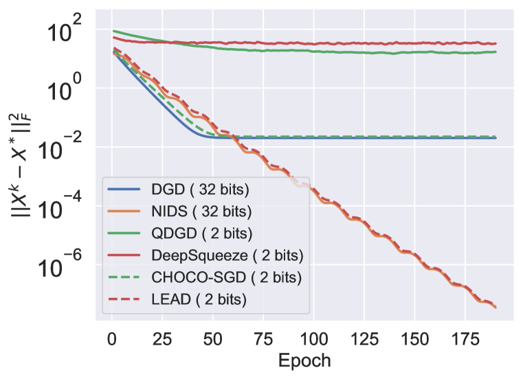
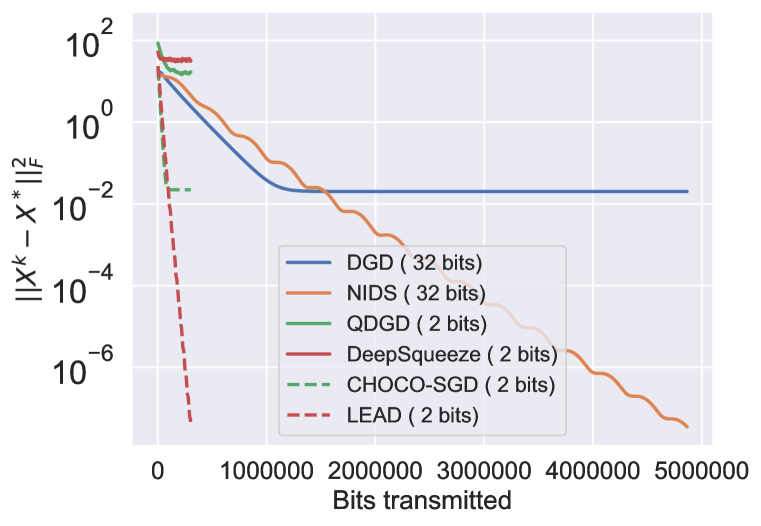
Linear regression. We consider the problem: f(𝒙)=i=1n(𝐀i𝒙𝒃i2+λ𝒙2)f({\bm{x}})=\sum_{i=1}^{n}(\|{\mathbf{A}}_{i}{\bm{x}}-{\bm{b}}_{i}\|^{2}+\lambda\|{\bm{x}}\|^{2}). Data matrices 𝐀i200×200{\mathbf{A}}_{i}\in\mathbb{R}^{200\times 200} and the true solution 𝒙{\bm{x}}^{\prime} is randomly synthesized. The values 𝒃i{\bm{b}}_{i} are generated by adding Gaussian noise to 𝐀i𝒙{\mathbf{A}}_{i}{\bm{x}}^{\prime}. We let λ=0.1\lambda=0.1 and the optimal solution of the linear regression problem be 𝒙{\bm{x}}^{*}. We use full-batch gradient to exclude the impact of gradient variance. The performance is showed in Fig. 1. The distance to 𝒙{\bm{x}}^{*} in Fig. 1a and the consensus error in Fig. 1c verify that LEAD converges exponentially to the optimal consensual solution. It significantly outperforms most baselines and matches NIDS well under the same number of iterations. Fig. 1b demonstrates the benefit of compression when considering the communication bits. Fig. 1d shows that the compression error vanishes for both LEAD and CHOCO-SGD while the compression error is pretty large for QDGD and DeepSqueeze because they directly compress the local models.
Refer to caption
(a) 𝐗k𝐗F\|{\mathbf{X}}^{k}-{\mathbf{X}}^{*}\|_{F}
Refer to caption
(b) 𝐗k𝐗F\|{\mathbf{X}}^{k}-{\mathbf{X}}^{*}\|_{F}
Refer to caption
(c) 𝐗k𝟏n×1𝐗¯kF\|{\mathbf{X}}^{k}-{{\bm{1}}_{n\times 1}\mkern 1.5mu\overline{\mkern-1.5mu{\mathbf{X}}\mkern-1.5mu}\mkern 1.5mu^{k}}\|_{F}
Refer to caption
(d) Compression error
Figure 1: Linear regression problem.

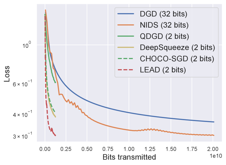
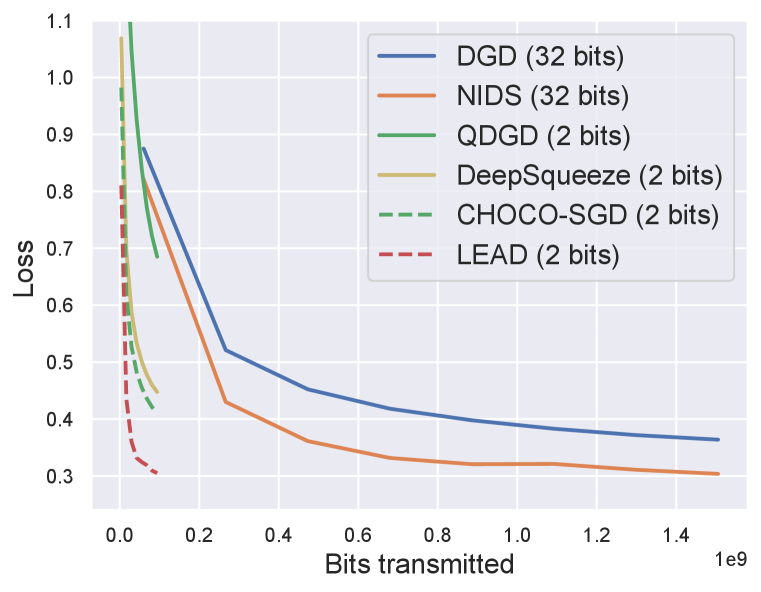
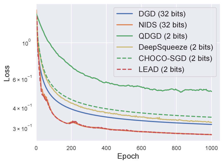
Logistic regression. We further consider a logistic regression problem on the MNIST dataset. The regularization parameter is 10410^{-4}. We consider both homogeneous and heterogeneous data settings. In the homogeneous setting, the data samples are randomly shuffled before being uniformly partitioned among all agents such that the data distribution from each agent is very similar. In the heterogeneous setting, the samples are first sorted by their labels and then partitioned among agents. Due to the space limit, we mainly present the results in heterogeneous setting here and defer the homogeneous setting to Appendix D.2. The results using full-batch gradient and mini-batch gradient (the mini-batch size is 512512 for each agent) are showed in Fig. 2 and Fig. 3 respectively and both settings shows the faster convergence and higher precision of LEAD.
Refer to caption
(a) Loss f(𝐗¯k)f(\mkern 1.5mu\overline{\mkern-1.5mu{\mathbf{X}}\mkern-1.5mu}\mkern 1.5mu^{k})
Refer to caption
(b) Loss f(𝐗¯k)f(\mkern 1.5mu\overline{\mkern-1.5mu{\mathbf{X}}\mkern-1.5mu}\mkern 1.5mu^{k})
Figure 2: Logistic regression problem in the heterogeneous case (full-batch gradient).
Refer to caption
(a) Loss f(𝐗¯k)f(\mkern 1.5mu\overline{\mkern-1.5mu{\mathbf{X}}\mkern-1.5mu}\mkern 1.5mu^{k})
Refer to caption
(b) Loss f(𝐗¯k)f(\mkern 1.5mu\overline{\mkern-1.5mu{\mathbf{X}}\mkern-1.5mu}\mkern 1.5mu^{k})
Figure 3: Logistic regression in the heterogeneous case (mini-batch gradient).
Refer to caption
(a) Loss f(𝐗¯k)f(\mkern 1.5mu\overline{\mkern-1.5mu{\mathbf{X}}\mkern-1.5mu}\mkern 1.5mu^{k})
Refer to caption
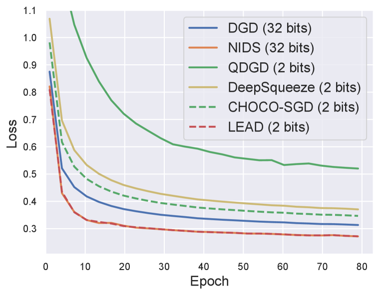
(b) Loss f(𝐗¯k)f(\mkern 1.5mu\overline{\mkern-1.5mu{\mathbf{X}}\mkern-1.5mu}\mkern 1.5mu^{k})
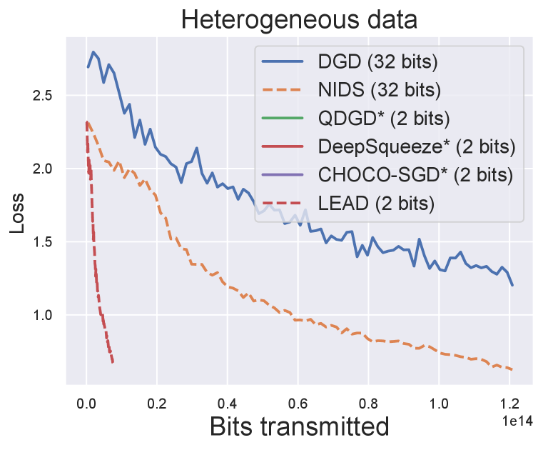
Figure 4: Stochastic optimization on deep neural network (* means divergence).

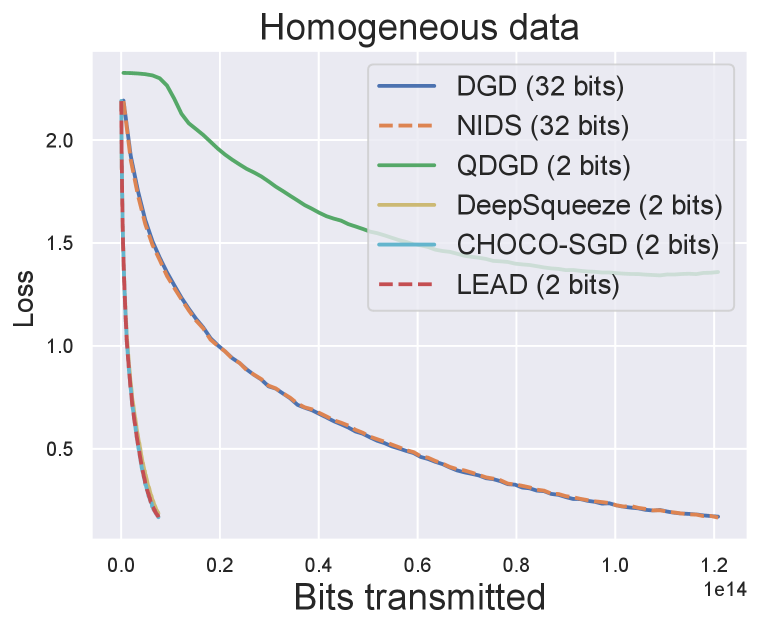
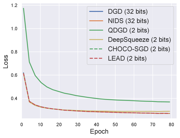
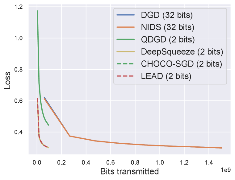
Neural network. We empirically study the performance of LEAD in optimizing deep neural network by training AlexNet (240240 MB) on CIFAR10 dataset. The mini-batch size is 6464 for each agents. Both the homogeneous and heterogeneous case are showed in Fig. 4. In the homogeneous case, CHOCO-SGD, DeepSqueeze and LEAD perform similarly and outperform the non-compressed variants in terms of communication efficiency, but CHOCO-SGD and DeepSqueeze need more efforts for parameter tuning because their convergence is sensitive to the setting of γ\gamma. In the heterogeneous cases, LEAD achieves the fastest and most stable convergence. Note that in this setting, sufficient information exchange is more important for convergence because models from different agents are moving to significantly diverse directions. In such case, DGD only converges with smaller stepsize and its communication compressed variants, including QDGD, DeepSqueeze and CHOCO-SGD, diverge in all parameter settings we try.

In summary, our experiments verify our theoretical analysis and show that LEAD is able to handle data heterogeneity very well. Furthermore, the performance of LEAD is robust to parameter settings and needs less effort for parameter tuning, which is critical in real-world applications.

6 Conclusion

In this paper, we investigate the communication compression in decentralized optimization. Motivated by primal-dual algorithms, a novel decentralized algorithm with compression, LEAD, is proposed to achieve faster convergence rate and to better handle heterogeneous data while enjoying the benefit of efficient communication. The nontrivial analyses on the coupled dynamics of inexact primal and dual updates as well as compression error establish the linear convergence of LEAD when full gradient is used and the linear convergence to the 𝒪(σ2)\mathcal{O}(\sigma^{2}) neighborhood of the optimum when stochastic gradient is used. Extensive experiments validate the theoretical analysis and demonstrate the state-of-the-art efficiency and robustness of LEAD. LEAD is also applicable to non-convex problems as empirically verified in the neural network experiments but we leave the non-convex analysis as the future work.

Acknowledgements

Xiaorui Liu and Dr. Jiliang Tang are supported by the National Science Foundation (NSF) under grant numbers CNS-1815636, IIS-1928278, IIS-1714741, IIS-1845081, IIS-1907704, and IIS-1955285. Yao Li and Dr. Ming Yan are supported by NSF grant DMS-2012439 and Facebook Faculty Research Award (Systems for ML). Dr. Rongrong Wang is supported by NSF grant CCF-1909523.

References

  • Alistarh et al. (2017) Dan Alistarh, Demjan Grubic, Jerry Li, Ryota Tomioka, and Milan Vojnovic. QSGD: Communication-efficient sgd via gradient quantization and encoding. In Advances in Neural Information Processing Systems, pp. 1709–1720. 2017.
  • Bernstein et al. (2018) Jeremy Bernstein, Yu-Xiang Wang, Kamyar Azizzadenesheli, and Animashree Anandkumar. SIGNSGD: compressed optimisation for non-convex problems. In Proceedings of the 35th International Conference on Machine Learning, pp.  559–568, 2018.
  • Carli et al. (2010) Ruggero Carli, Fabio Fagnani, Paolo Frasca, and Sandro Zampieri. Gossip consensus algorithms via quantized communication. Automatica, 46(1):70–80, 2010.
  • Karimireddy et al. (2019) Sai Praneeth Karimireddy, Quentin Rebjock, Sebastian Urban Stich, and Martin Jaggi. Error feedback fixes SignSGD and other gradient compression schemes. In Proceedings of the 36th International Conference on Machine Learning, pp.  3252–3261. PMLR, 2019.
  • Koloskova et al. (2019) Anastasia Koloskova, Sebastian U. Stich, and Martin Jaggi. Decentralized stochastic optimization and gossip algorithms with compressed communication. In Proceedings of the 36th International Conference on Machine Learning, pp.  3479–3487. PMLR, 2019.
  • Koloskova et al. (2020) Anastasia Koloskova, Tao Lin, Sebastian U Stich, and Martin Jaggi. Decentralized deep learning with arbitrary communication compression. In International Conference on Learning Representations, 2020.
  • Li & Yan (2019) Yao Li and Ming Yan. On linear convergence of two decentralized algorithms. arXiv preprint arXiv:1906.07225, 2019.
  • Li et al. (2019) Zhi Li, Wei Shi, and Ming Yan. A decentralized proximal-gradient method with network independent step-sizes and separated convergence rates. IEEE Transactions on Signal Processing, 67(17):4494–4506, 2019.
  • Lian et al. (2017) Xiangru Lian, Ce Zhang, Huan Zhang, Cho-Jui Hsieh, Wei Zhang, and Ji Liu. Can decentralized algorithms outperform centralized algorithms? a case study for decentralized parallel stochastic gradient descent. In Advances in Neural Information Processing Systems, pp. 5330–5340, 2017.
  • Ling et al. (2015) Qing Ling, Wei Shi, Gang Wu, and Alejandro Ribeiro. DLM: Decentralized linearized alternating direction method of multipliers. IEEE Transactions on Signal Processing, 63(15):4051–4064, 2015.
  • Liu et al. (2020) Xiaorui Liu, Yao Li, Jiliang Tang, and Ming Yan. A double residual compression algorithm for efficient distributed learning. The 23rd International Conference on Artificial Intelligence and Statistics, 2020.
  • Lu & De Sa (2020) Yucheng Lu and Christopher De Sa. Moniqua: Modulo quantized communication in decentralized SGD. In Proceedings of the 37th International Conference on Machine Learning, 2020.
  • Magnússon et al. (2020) Sindri Magnússon, Hossein Shokri-Ghadikolaei, and Na Li. On maintaining linear convergence of distributed learning and optimization under limited communication. IEEE Transactions on Signal Processing, 68:6101–6116, 2020.
  • Mishchenko et al. (2019) Konstantin Mishchenko, Eduard Gorbunov, Martin Takáč, and Peter Richtárik. Distributed learning with compressed gradient differences. arXiv preprint arXiv:1901.09269, 2019.
  • Mota et al. (2013) Joao FC Mota, Joao MF Xavier, Pedro MQ Aguiar, and Markus Püschel. D-ADMM: A communication-efficient distributed algorithm for separable optimization. IEEE Transactions on Signal Processing, 61(10):2718–2723, 2013.
  • Nedic & Ozdaglar (2009) Angelia Nedic and Asuman Ozdaglar. Distributed subgradient methods for multi-agent optimization. IEEE Transactions on Automatic Control, 54(1):48–61, 2009.
  • Nedic et al. (2017) Angelia Nedic, Alex Olshevsky, and Wei Shi. Achieving geometric convergence for distributed optimization over time-varying graphs. SIAM Journal on Optimization, 27(4):2597–2633, 2017.
  • Nesterov (2013) Yurii Nesterov. Introductory lectures on convex optimization: A basic course, volume 87. Springer Science & Business Media, 2013.
  • Pu & Nedić (2020) Shi Pu and Angelia Nedić. Distributed stochastic gradient tracking methods. Mathematical Programming, pp.  1–49, 2020.
  • Reisizadeh et al. (2019a) Amirhossein Reisizadeh, Aryan Mokhtari, Hamed Hassani, and Ramtin Pedarsani. An exact quantized decentralized gradient descent algorithm. IEEE Transactions on Signal Processing, 67(19):4934–4947, 2019a.
  • Reisizadeh et al. (2019b) Amirhossein Reisizadeh, Hossein Taheri, Aryan Mokhtari, Hamed Hassani, and Ramtin Pedarsani. Robust and communication-efficient collaborative learning. In Advances in Neural Information Processing Systems, pp. 8388–8399, 2019b.
  • Seide et al. (2014) Frank Seide, Hao Fu, Jasha Droppo, Gang Li, and Dong Yu. 1-bit stochastic gradient descent and application to data-parallel distributed training of speech DNNs. In Interspeech 2014, September 2014.
  • Shi et al. (2015) Wei Shi, Qing Ling, Gang Wu, and Wotao Yin. EXTRA: An exact first-order algorithm for decentralized consensus optimization. SIAM Journal on Optimization, 25(2):944–966, 2015.
  • Stich et al. (2018) Sebastian U. Stich, Jean-Baptiste Cordonnier, and Martin Jaggi. Sparsified SGD with memory. In Proceedings of the 32nd International Conference on Neural Information Processing Systems, pp.  4452–4463, 2018.
  • Tang et al. (2018a) Hanlin Tang, Shaoduo Gan, Ce Zhang, Tong Zhang, and Ji Liu. Communication compression for decentralized training. In Advances in Neural Information Processing Systems, pp. 7652–7662. 2018a.
  • Tang et al. (2018b) Hanlin Tang, Xiangru Lian, Ming Yan, Ce Zhang, and Ji Liu. D2D^{2}: Decentralized training over decentralized data. In Proceedings of the 35th International Conference on Machine Learning, pp.  4848–4856, 2018b.
  • Tang et al. (2019a) Hanlin Tang, Xiangru Lian, Shuang Qiu, Lei Yuan, Ce Zhang, Tong Zhang, and Ji Liu. Deepsqueeze: Decentralization meets error-compensated compression. CoRR, abs/1907.07346, 2019a. URL http://arxiv.org/abs/1907.07346.
  • Tang et al. (2019b) Hanlin Tang, Chen Yu, Xiangru Lian, Tong Zhang, and Ji Liu. DoubleSqueeze: Parallel stochastic gradient descent with double-pass error-compensated compression. In Proceedings of the 36th International Conference on Machine Learning, pp.  6155–6165, 2019b.
  • Tsitsiklis et al. (1986) John Tsitsiklis, Dimitri Bertsekas, and Michael Athans. Distributed asynchronous deterministic and stochastic gradient optimization algorithms. IEEE transactions on automatic control, 31(9):803–812, 1986.
  • Wu et al. (2018) Jiaxiang Wu, Weidong Huang, Junzhou Huang, and Tong Zhang. Error compensated quantized SGD and its applications to large-scale distributed optimization. In Proceedings of the 35th International Conference on Machine Learning, pp.  5325–5333, 2018.
  • Xiao & Boyd (2004) Lin Xiao and Stephen Boyd. Fast linear iterations for distributed averaging. Systems & Control Letters, 53(1):65–78, 2004.
  • Xu et al. (2020) Jinming Xu, Ye Tian, Ying Sun, and Gesualdo Scutari. Accelerated primal-dual algorithms for distributed smooth convex optimization over networks. In International Conference on Artificial Intelligence and Statistics, pp.  2381–2391. PMLR, 2020.
  • Yuan et al. (2016) Kun Yuan, Qing Ling, and Wotao Yin. On the convergence of decentralized gradient descent. SIAM Journal on Optimization, 26(3):1835–1854, 2016.
  • Yuan et al. (2018) Kun Yuan, Bicheng Ying, Xiaochuan Zhao, and Ali H Sayed. Exact diffusion for distributed optimization and learning—part i: Algorithm development. IEEE Transactions on Signal Processing, 67(3):708–723, 2018.
  • Yuan et al. (2020) Kun Yuan, Wei Xu, and Qing Ling. Can primal methods outperform primal-dual methods in decentralized dynamic optimization? arXiv preprint arXiv:2003.00816, 2020.
\etocsettocstyle

Contents of Appendix


\etocdepthtag

.tocmtappendix \etocsettagdepthmtchapternone \etocsettagdepthmtappendixsubsection

Appendix A LEAD in agent’s perspective

In the main paper, we described the algorithm with matrix notations for concision. Here we further provide a complete algorithm description from the agents’ perspective.

Algorithm 2 LEAD in Agent’s Perspective

input: stepsize η\eta, compression parameters (α,γ\alpha,~{}\gamma), initial values 𝒙i0{\bm{x}}_{i}^{0}𝒉i1{\bm{h}}_{i}^{1}𝒛i,i{1,2,,n}{\bm{z}}_{i},~{}\forall i\in\{1,2,\dots,n\}
output: 𝒙iK,i{1,2,,n}{\bm{x}}_{i}^{K},~{}\forall i\in\{1,2,\dots,n\} or i=1n𝒙iKn\frac{\sum_{i=1}^{n}{\bm{x}}_{i}^{K}}{n}

1:for each agent i{1,2,,n}i\in\{1,2,\dots,n\} do
2:     𝒅i1=𝒛ij𝒩i{i}wij𝒛j{\bm{d}}_{i}^{1}={\bm{z}}_{i}-\sum_{j\in\mathcal{N}_{i}\cup\{i\}}w_{ij}{\bm{z}}_{j}
3:     (𝒉w)i1=j𝒩i{i}wij(𝒉w)j1({\bm{h}}_{w})_{i}^{1}=\sum_{j\in\mathcal{N}_{i}\cup\{i\}}w_{ij}({\bm{h}}_{w})_{j}^{1}
4:     𝒙i1=𝒙i0ηfi(𝒙i0;ξi0){\bm{x}}_{i}^{1}={\bm{x}}_{i}^{0}-\eta\nabla f_{i}({\bm{x}}_{i}^{0};\xi_{i}^{0})
5:end for
6:for k=1,2,,K1k=1,2,\dots,K-1 do in parallel for all agents i{1,2,,n}i\in\{1,2,\dots,n\}
7:     compute fi(𝒙ik;ξik)\nabla f_{i}({\bm{x}}_{i}^{k};\xi_{i}^{k}) \vartriangleright Gradient computation
8:     𝒚ik=𝒙ikηfi(𝒙ik;ξik)η𝒅ik{\bm{y}}_{i}^{k}={\bm{x}}_{i}^{k}-\eta\nabla f_{i}({\bm{x}}_{i}^{k};\xi^{k}_{i})-\eta{\bm{d}}_{i}^{k}
9:     𝒒ik=Compress(𝒚ik𝒉ik){\bm{q}}_{i}^{k}={\text{Compress}}({\bm{y}}_{i}^{k}-{\bm{h}}_{i}^{k}) \vartriangleright Compression
10:     𝒚^ik=𝒉ik+𝒒ik\hat{\bm{y}}_{i}^{k}={\bm{h}}_{i}^{k}+{\bm{q}}_{i}^{k}
11:     for neighbors j𝒩ij\in\mathcal{N}_{i} do
12:         Send 𝒒ik{\bm{q}}_{i}^{k} and receive 𝒒jk{\bm{q}}_{j}^{k} \vartriangleright Communication
13:     end for
14:     (𝒚^w)ik=(𝒉w)ik+j𝒩i{i}wij𝒒jk{(\hat{\bm{y}}_{w})}_{i}^{k}={({\bm{h}}_{w})}_{i}^{k}+\sum_{j\in\mathcal{N}_{i}\cup\{i\}}w_{ij}{\bm{q}}_{j}^{k}
15:     𝒉ik+1=(1α)𝒉ik+α𝒚^ik{\bm{h}}_{i}^{k+1}=(1-\alpha){\bm{h}}_{i}^{k}+\alpha\hat{\bm{y}}_{i}^{k}
16:     (𝒉w)ik+1=(1α)(𝒉w)ik+α(𝒚^w)ik{({\bm{h}}_{w})}_{i}^{k+1}=(1-\alpha){({\bm{h}}_{w})}_{i}^{k}+\alpha{(\hat{\bm{y}}_{w})}_{i}^{k}
17:     𝒅ik+1=𝒅ik+γ2η(𝒚^ik(𝒚^w)ik){\bm{d}}_{i}^{k+1}={\bm{d}}_{i}^{k}+\frac{\gamma}{2\eta}\big{(}\hat{\bm{y}}_{i}^{k}-{(\hat{\bm{y}}_{w})}_{i}^{k}\big{)}
18:     𝒙ik+1=𝒙ikηfi(𝒙ik;ξik)η𝒅ik+1{\bm{x}}_{i}^{k+1}={\bm{x}}_{i}^{k}-\eta\nabla f_{i}({\bm{x}}_{i}^{k};\xi_{i}^{k})-\eta{\bm{d}}_{i}^{k+1} \vartriangleright Model update
19:end for

Appendix B Connections with exiting works

The non-compressed variant of LEAD in Alg. 1 recovers NIDS (Li et al., 2019), D2D^{2} (Tang et al., 2018b) and Exact Diffusion (Yuan et al., 2018) as shown in Proposition 1. In Corollary 3, we show that the convergence rate of LEAD exactly recovers the rate of NIDS when C=0,γ=1C=0,\gamma=1 and σ=0\sigma=0.

Proposition 1 (Connection to NIDS, D2D^{2} and Exact Diffusion).

When there is no communication compression (i.e., 𝐘^k=𝐘k\hat{\mathbf{Y}}^{k}={\mathbf{Y}}^{k}) and γ=1\gamma=1, Alg. 1 recovers D2D^{2}:

𝐗k+1=𝐈+𝐖2(2𝐗k𝐗k1η𝐅(𝐗k;ξk)+η𝐅(𝐗k1;ξk1)).\displaystyle{\mathbf{X}}^{k+1}=\frac{{\mathbf{I}}+{\mathbf{W}}}{2}\Big{(}2{\mathbf{X}}^{k}-{\mathbf{X}}^{k-1}-\eta\nabla{\mathbf{F}}({\mathbf{X}}^{k};\xi^{k})+\eta\nabla{\mathbf{F}}({\mathbf{X}}^{k-1};\xi^{k-1})\Big{)}. (15)

Furthermore, if the stochastic estimator of the gradient 𝐅(𝐗k;ξk)\nabla{\mathbf{F}}({\mathbf{X}}^{k};\xi^{k}) is replaced by the full gradient, it recovers NIDS and Exact Diffusion with specific settings.

Corollary 3 (Consistency with NIDS).

When C=0C=0 (no communication compression), γ=1\gamma=1 and σ=0\sigma=0 (full gradient), LEAD has the convergence consistent with NIDS with η(0,2/(μ+L)]\eta\in(0,2/(\mu+L)]:

k+1max{1μ(2ημη2),112λmax((𝐈𝐖))}k.\displaystyle\mathcal{L}^{k+1}\leq\max\left\{1-\mu(2\eta-\mu\eta^{2}),1-\frac{1}{2\lambda_{\max}(({\mathbf{I}}-{\mathbf{W}})^{\dagger})}\right\}\mathcal{L}^{k}. (16)

See the proof in E.5.

Proof of Proposition 1.

Let γ=1\gamma=1 and 𝐘^k=𝐘k\hat{\mathbf{Y}}^{k}={\mathbf{Y}}^{k}. Combing Lines 4 and 6 of Alg. 1 gives

𝐃k+1\displaystyle{\mathbf{D}}^{k+1} =𝐃k+𝐈𝐖2η(𝐗kη𝐅(𝐗k;ξk)η𝐃k).\displaystyle={\mathbf{D}}^{k}+\frac{{\mathbf{I}}-{\mathbf{W}}}{2\eta}({\mathbf{X}}^{k}-\eta\nabla{\mathbf{F}}({\mathbf{X}}^{k};\xi^{k})-\eta{\mathbf{D}}^{k}). (17)

Based on Line 7, we can represent η𝐃k\eta{\mathbf{D}}^{k} from the previous iteration as

η𝐃k=𝐗k1𝐗kη𝐅(𝐗k1;ξk1).\displaystyle\eta{\mathbf{D}}^{k}={\mathbf{X}}^{k-1}-{\mathbf{X}}^{k}-\eta\nabla{\mathbf{F}}({\mathbf{X}}^{k-1};\xi^{k-1}). (18)

Eliminating both 𝐃k{\mathbf{D}}^{k} and 𝐃k+1{\mathbf{D}}^{k+1} by substituting (17)-(18) into Line 7, we obtain

𝐗k+1\displaystyle{\mathbf{X}}^{k+1} =𝐗kη𝐅(𝐗k;ξk)(η𝐃k+𝐈𝐖2(𝐗kη𝐅(𝐗k;ξk)η𝐃k))(from(17))\displaystyle={\mathbf{X}}^{k}-\eta\nabla{\mathbf{F}}({\mathbf{X}}^{k};\xi^{k})-\Big{(}\eta{\mathbf{D}}^{k}+\frac{{\mathbf{I}}-{\mathbf{W}}}{2}({\mathbf{X}}^{k}-\eta\nabla{\mathbf{F}}({\mathbf{X}}^{k};\xi^{k})-\eta{\mathbf{D}}^{k})\Big{)}\quad(\text{from}~{}(\ref{equ:nids_1}))
=𝐈+𝐖2(𝐗kη𝐅(𝐗k;ξk))𝐈+𝐖2η𝐃k\displaystyle=\frac{{\mathbf{I}}+{\mathbf{W}}}{2}({\mathbf{X}}^{k}-\eta\nabla{\mathbf{F}}({\mathbf{X}}^{k};\xi^{k}))-\frac{{\mathbf{I}}+{\mathbf{W}}}{2}\eta{\mathbf{D}}^{k}
=𝐈+𝐖2(𝐗kη𝐅(𝐗k;ξk))𝐈+𝐖2(𝐗k1𝐗kη𝐅(𝐗k1;ξk1))(from(18))\displaystyle=\frac{{\mathbf{I}}+{\mathbf{W}}}{2}({\mathbf{X}}^{k}-\eta\nabla{\mathbf{F}}({\mathbf{X}}^{k};\xi^{k}))-\frac{{\mathbf{I}}+{\mathbf{W}}}{2}({\mathbf{X}}^{k-1}-{\mathbf{X}}^{k}-\eta\nabla{\mathbf{F}}({\mathbf{X}}^{k-1};\xi^{k-1}))\quad(\text{from}~{}(\ref{equ:nids_2}))
=𝐈+𝐖2(2𝐗k𝐗k1η𝐅(𝐗k;ξk)+η𝐅(𝐗k1;ξk1)),\displaystyle=\frac{{\mathbf{I}}+{\mathbf{W}}}{2}(2{\mathbf{X}}^{k}-{\mathbf{X}}^{k-1}-\eta\nabla{\mathbf{F}}({\mathbf{X}}^{k};\xi^{k})+\eta\nabla{\mathbf{F}}({\mathbf{X}}^{k-1};\xi^{k-1})), (19)

which is exactly D2D^{2}. It also recovers Exact Diffusion with 𝐀=𝐈+𝐖2{\mathbf{A}}=\frac{{\mathbf{I}}+{\mathbf{W}}}{2} and 𝐌=η𝐈{\mathbf{M}}=\eta{\mathbf{I}} in Eq. (97) of (Yuan et al., 2018). ∎

Appendix C Compression method

C.1 p-norm b-bits quantization

Theorem 3 (p-norm b-bit quantization).

Let us define the quantization operator as

Qp(𝒙):=(𝒙psign(𝒙)2(b1))2b1|𝒙|𝒙p+𝒖\displaystyle Q_{p}({\bm{x}}):=\left(\|{\bm{x}}\|_{p}\operatorname{sign}({\bm{x}})2^{-(b-1)}\right)\cdot\left\lfloor{\frac{2^{b-1}|{\bm{x}}|}{\|{\bm{x}}\|_{p}}+{\bm{u}}}\right\rfloor (20)

where \cdot is the Hadamard product, |𝐱||{\bm{x}}| is the elementwise absolute value and 𝐮{\bm{u}} is a random dither vector uniformly distributed in [0,1]d[0,1]^{d}. Qp(𝐱)Q_{p}({\bm{x}}) is unbiased, i.e., 𝔼Qp(𝐱)=𝐱{\mathbb{E}}Q_{p}({\bm{x}})={\bm{x}}, and the compression variance is upper bounded by

𝔼𝒙Qp(𝒙)214sign(𝒙)2(b1)2𝒙p2,\displaystyle{\mathbb{E}}\|{\bm{x}}-Q_{p}({\bm{x}})\|^{2}\leq\frac{1}{4}\|\operatorname{sign}({\bm{x}})2^{-(b-1)}\|^{2}\|{\bm{x}}\|_{p}^{2}, (21)

which suggests that \infty-norm provides the smallest upper bound for the compression variance due to 𝐱p𝐱q,𝐱\|{\bm{x}}\|_{p}\leq\|{\bm{x}}\|_{q},\forall{\bm{x}} if 1qp1\leq q\leq p\leq\infty.

Remark 7.

For the compressor defined in (20), we have the following the compression constant

C=sup𝒙sign(𝒙)2(b1)2𝒙p24𝒙2.C=\sup_{{\bm{x}}}\frac{\|\operatorname{sign}({\bm{x}})2^{-(b-1)}\|^{2}\|{\bm{x}}\|_{p}^{2}}{4\|{\bm{x}}\|^{2}}.
Proof.

Let denote 𝒗=𝒙psign(𝒙)2(b1){\bm{v}}=\|{\bm{x}}\|_{p}\operatorname{sign}({\bm{x}})2^{-(b-1)}, s=2b1|𝒙|𝒙ps=\frac{2^{b-1}|{\bm{x}}|}{\|{\bm{x}}\|_{p}}, s1=2b1|𝒙|𝒙ps_{1}=\left\lfloor{\frac{2^{b-1}|{\bm{x}}|}{\|{\bm{x}}\|_{p}}}\right\rfloor and s2=2b1|𝒙|𝒙ps_{2}=\left\lceil{\frac{2^{b-1}|{\bm{x}}|}{\|{\bm{x}}\|_{p}}}\right\rceil. We can rewrite 𝒙{\bm{x}} as 𝒙=s𝒗{\bm{x}}=s\cdot{\bm{v}}.

For any coordinate ii such that si=(s1)is_{i}=(s_{1})_{i}, we have Qp(𝒙i)=(s1)i𝒗iQ_{p}({\bm{x}}_{i})=(s_{1})_{i}{\bm{v}}_{i} with probability 11. Hence 𝔼Qp(𝒙)i=si𝒗i=𝒙i{\mathbb{E}}Q_{p}({\bm{x}})_{i}=s_{i}{\bm{v}}_{i}={\bm{x}}_{i} and

𝔼(𝒙iQp(𝒙)i)2=(𝒙isi𝒗i)2=0.\displaystyle{\mathbb{E}}({\bm{x}}_{i}-Q_{p}({\bm{x}})_{i})^{2}=({\bm{x}}_{i}-s_{i}{\bm{v}}_{i})^{2}=0.

For any coordinate ii such that si(s1)is_{i}\not=(s_{1})_{i}, we have (s2)i(s1)i=1(s_{2})_{i}-(s_{1})_{i}=1 and Qp(𝒙)iQ_{p}({\bm{x}})_{i} satisfies

Qp(𝒙)i={(s1)i𝒗i,w.p.(s2)isi,(s2)i𝒗i,w.p.si(s1)i.Q_{p}({\bm{x}})_{i}=\left\{\begin{aligned} &(s_{1})_{i}{\bm{v}}_{i},\ \ \text{w.p.}\ (s_{2})_{i}-s_{i},\\ &(s_{2})_{i}{\bm{v}}_{i},\ \ \text{w.p.}\ s_{i}-(s_{1})_{i}.\\ \end{aligned}\right.

Thus, we derive

𝔼Qp(𝒙)i\displaystyle{\mathbb{E}}Q_{p}({\bm{x}})_{i} =𝒗i(s1)i(s2s)i+𝒗i(s2)i(ss1)i=𝒗isi(s2s1)i=𝒗isi=𝒙i,\displaystyle={\bm{v}}_{i}(s_{1})_{i}(s_{2}-s)_{i}+{\bm{v}}_{i}(s_{2})_{i}(s-s_{1})_{i}={\bm{v}}_{i}s_{i}(s_{2}-s_{1})_{i}={\bm{v}}_{i}s_{i}={\bm{x}}_{i},

and

𝔼[𝒙iQp(𝒙)i]2\displaystyle{\mathbb{E}}[{\bm{x}}_{i}-Q_{p}({\bm{x}})_{i}]^{2} =(𝒙i𝒗i(s1)i)2(s2s)i+(𝒙i𝒗i(s2)i)2(ss1)i\displaystyle=({\bm{x}}_{i}-{\bm{v}}_{i}(s_{1})_{i})^{2}(s_{2}-s)_{i}+({\bm{x}}_{i}-{\bm{v}}_{i}(s_{2})_{i})^{2}(s-s_{1})_{i}
=(s2s1)i𝒙i2+((s1)i(s2)i(s1s2)i+si((s2)i2(s1)i2))𝒗i22si(s2s1)i𝒙i𝒗i\displaystyle=(s_{2}-s_{1})_{i}{\bm{x}}_{i}^{2}+\big{(}(s_{1})_{i}(s_{2})_{i}(s_{1}-s_{2})_{i}+s_{i}((s_{2})_{i}^{2}-(s_{1})_{i}^{2})\big{)}{\bm{v}}_{i}^{2}-2s_{i}(s_{2}-s_{1})_{i}{\bm{x}}_{i}{\bm{v}}_{i}
=𝒙i2+((s1)i(s2)i+si(s2+s1)i)𝒗i22si𝒙i𝒗i\displaystyle={\bm{x}}_{i}^{2}+\big{(}-(s_{1})_{i}(s_{2})_{i}+s_{i}(s_{2}+s_{1})_{i}\big{)}{\bm{v}}_{i}^{2}-2s_{i}{\bm{x}}_{i}{\bm{v}}_{i}
=(𝒙isi𝒗i)2+((s1)i(s2)i+si(s2+s1)isi2)𝒗i2\displaystyle=({\bm{x}}_{i}-s_{i}{\bm{v}}_{i})^{2}+\big{(}-(s_{1})_{i}(s_{2})_{i}+s_{i}(s_{2}+s_{1})_{i}-s_{i}^{2}\big{)}{\bm{v}}_{i}^{2}
=(𝒙isi𝒗i)2+(s2s)i(ss1)i𝒗i2\displaystyle=({\bm{x}}_{i}-s_{i}{\bm{v}}_{i})^{2}+(s_{2}-s)_{i}(s-s_{1})_{i}{\bm{v}}_{i}^{2}
=(s2s)i(ss1)i𝒗i2\displaystyle=(s_{2}-s)_{i}(s-s_{1})_{i}{\bm{v}}_{i}^{2}
14𝒗i2.\displaystyle\leq\frac{1}{4}{\bm{v}}_{i}^{2}.

Considering both cases, we have 𝔼Q(𝒙)=𝒙{\mathbb{E}}Q({\bm{x}})={\bm{x}} and

𝔼𝒙Qp(𝒙)2\displaystyle{\mathbb{E}}\|{\bm{x}}-Q_{p}({\bm{x}})\|^{2} ={si=(s1)i}𝔼[𝒙iQp(𝒙)i]2+{si(s1)i}𝔼[𝒙iQp(𝒙)i]2\displaystyle=\sum_{\{s_{i}=(s_{1})_{i}\}}{\mathbb{E}}[{\bm{x}}_{i}-Q_{p}({\bm{x}})_{i}]^{2}+\sum_{\{s_{i}\not=(s_{1})_{i}\}}{\mathbb{E}}[{\bm{x}}_{i}-Q_{p}({\bm{x}})_{i}]^{2}
0+14{si(s1)i}𝒗i2\displaystyle\leq 0+\frac{1}{4}\sum_{\{s_{i}\not=(s_{1})_{i}\}}{\bm{v}}_{i}^{2}
14𝒗2\displaystyle\leq\frac{1}{4}\|{\bm{v}}\|^{2}
=14sign(𝒙)2(b1)2𝒙p2.\displaystyle=\frac{1}{4}\|\operatorname{sign}({\bm{x}})2^{-(b-1)}\|^{2}\|{\bm{x}}\|_{p}^{2}.

C.2 Compression error

Refer to caption
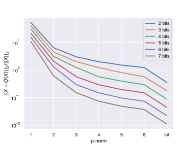
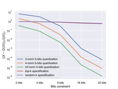
Figure 5: Relative compression error 𝒙Q(𝒙)2𝒙2\frac{\|{\bm{x}}-Q({\bm{x}})\|_{2}}{\|{\bm{x}}\|_{2}} for p-norm b-bit quantization
Refer to caption
Figure 6: Comparison of compression error 𝒙Q(𝒙)2𝒙2\frac{\|{\bm{x}}-Q({\bm{x}})\|_{2}}{\|{\bm{x}}\|_{2}} between different compression methods

To verify Theorem 3, we compare the compression error of the quantization method defined in (20) with different norms (p=1,2,3,,6,p=1,2,3,\dots,6,\infty). Specifically, we uniformly generate 100 random vectors in 10000\mathbb{R}^{10000} and compute the average compression error. The result shown in Figure 5 verifies our proof in Theorem 3 that the compression error decreases when pp increases. This suggests that \infty-norm provides the best compression precision under the same bit constraint.

Under similar setting, we also compare the compression error with other popular compression methods, such as top-k and random-k sparsification. The x-axes represents the average bits needed to represent each element of the vector. The result is showed in Fig. 6. Note that intuitively top-k methods should perform better than random-k method, but the top-k method needs extra bits to transmitted the index while random-k method can avoid this by using the same random seed. Therefore, top-k method doesn’t outperform random-k too much under the same communication budget. The result in Fig. 6 suggests that \infty-norm b-bits quantization provides significantly better compression precision than others under the same bit constraint.

Appendix D Experiments

D.1 Parameter sensitivity

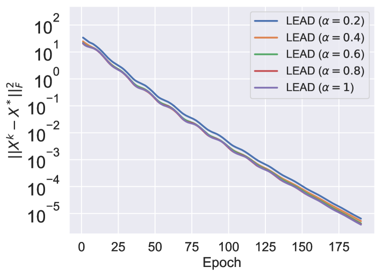
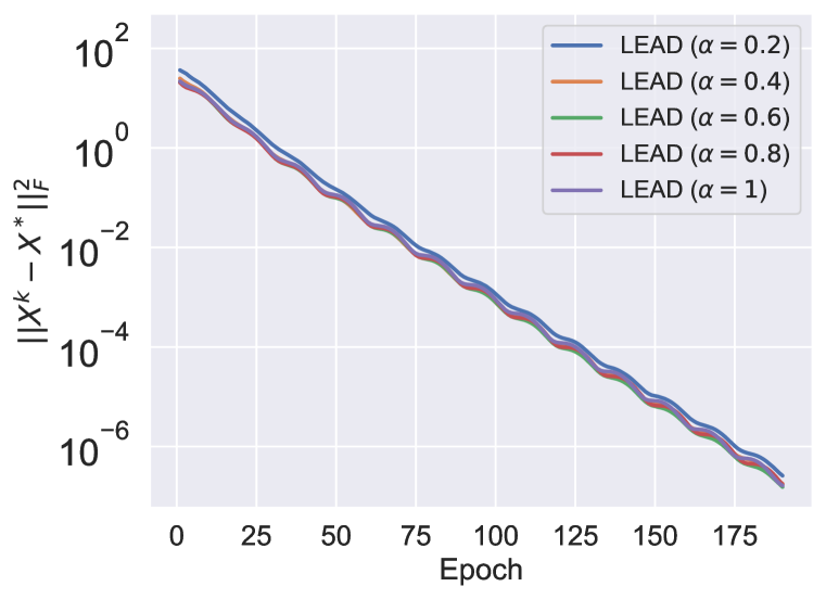
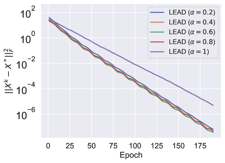
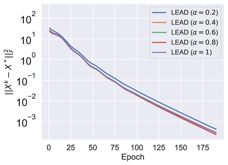
In the linear regression problem, the convergence of LEAD under different parameter settings of α\alpha and γ\gamma are tested. The result showed in Figure 7 indicates that LEAD performs well in most settings and is robust to the parameter setting. Therefore, in this paper, we simply set α=0.5\alpha=0.5 and γ=1.0\gamma=1.0 for LEAD in all experiment, which indicates the minor effort needed for parameter tuning.
Refer to caption
(a) γ=0.4\gamma=0.4
Refer to caption
(b) γ=0.6\gamma=0.6
Refer to caption
(c) γ=0.8\gamma=0.8
Refer to caption
(d) γ=1.0\gamma=1.0
Figure 7: Parameter analysis on linear regression problem.

D.2 Experiments in homogeneous setting

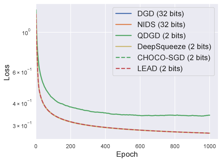
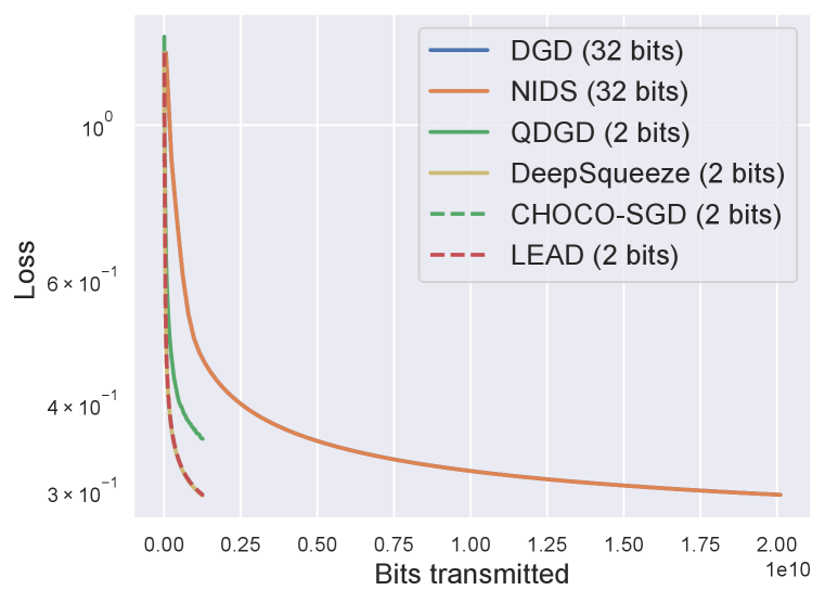
The experiments on logistic regression problem in homogeneous case are showed in Fig. 8 and Fig. 9. It shows that DeepSqueeze, CHOCO-SGD and LEAD converges similarly while DeepSqueeze and CHOCO-SGD require to tune a smaller γ\gamma for convergence as showed in the parameter setting in Section D.3. Generally, a smaller γ\gamma decreases the model propagation between agents since γ\gamma changes the effective mixing matrix and this may cause slower convergence. However, in the setting where data from different agents are very similar, the models move to close directions such that the convergence is not affected too much.
Refer to caption
(a) Loss f(𝐗¯k)f(\mkern 1.5mu\overline{\mkern-1.5mu{\mathbf{X}}\mkern-1.5mu}\mkern 1.5mu^{k})
Refer to caption
(b) Loss f(𝐗¯k)f(\mkern 1.5mu\overline{\mkern-1.5mu{\mathbf{X}}\mkern-1.5mu}\mkern 1.5mu^{k})
Figure 8: Logistic regression in the homogeneous case (full-batch gradient)
Refer to caption
(a) Loss f(𝐗¯k)f(\mkern 1.5mu\overline{\mkern-1.5mu{\mathbf{X}}\mkern-1.5mu}\mkern 1.5mu^{k})
Refer to caption
(b) Loss f(𝐗¯k)f(\mkern 1.5mu\overline{\mkern-1.5mu{\mathbf{X}}\mkern-1.5mu}\mkern 1.5mu^{k})
Figure 9: Logistic regression in the homogeneous case (mini-batch gradient)

D.3 Parameter settings

The best parameter settings we search for all algorithms and experiments are summarized in Tables 1– 10. QDGD and DeepSqueeze are more sensitive to γ\gamma and CHOCO-SGD is slight more robust. LEAD is most robust to parameter settings and it works well for the setting α=0.5\alpha=0.5 and γ=1.0\gamma=1.0 in all experiments in this paper.

Algorithm η\eta γ\gamma α\alpha
DGD 0.10.1 - -
NIDS 0.10.1 - -
QDGD 0.10.1 0.20.2 -
DeepSqueeze 0.10.1 0.20.2 -
CHOCO-SGD 0.10.1 0.80.8 -
LEAD 0.10.1 1.01.0 0.50.5
Table 1: Parameter settings for the linear regression problem.
Algorithm η\eta γ\gamma α\alpha
DGD 0.10.1 - -
NIDS 0.10.1 - -
QDGD 0.10.1 0.40.4 -
DeepSqueeze 0.10.1 0.40.4 -
CHOCO-SGD 0.10.1 0.60.6 -
LEAD 0.10.1 1.01.0 0.50.5
Table 2: *

Homogeneous case

Algorithm η\eta γ\gamma α\alpha
DGD 0.10.1 - -
NIDS 0.10.1 - -
QDGD 0.10.1 0.20.2 -
DeepSqueeze 0.10.1 0.60.6 -
CHOCO-SGD 0.10.1 0.60.6 -
LEAD 0.10.1 1.01.0 0.50.5
Table 3: *

Heterogeneous case

Table 4: Parameter settings for the logistic regression problem (full-batch gradient).
Algorithm η\eta γ\gamma α\alpha
DGD 0.10.1 - -
NIDS 0.10.1 - -
QDGD 0.050.05 0.20.2 -
DeepSqueeze 0.10.1 0.60.6 -
CHOCO-SGD 0.10.1 0.60.6 -
LEAD 0.10.1 1.01.0 0.50.5
Table 5: *

Homogeneous case

Algorithm η\eta γ\gamma α\alpha
DGD 0.10.1 - -
NIDS 0.10.1 - -
QDGD 0.050.05 0.20.2 -
DeepSqueeze 0.10.1 0.60.6 -
CHOCO-SGD 0.10.1 0.60.6 -
LEAD 0.10.1 1.01.0 0.50.5
Table 6: *

Heterogeneous case

Table 7: Parameter settings for the logistic regression problem (mini-batch gradient).
Algorithm η\eta γ\gamma α\alpha
DGD 0.10.1 - -
NIDS 0.10.1 - -
QDGD 0.050.05 0.10.1 -
DeepSqueeze 0.10.1 0.20.2 -
CHOCO-SGD 0.10.1 0.60.6 -
LEAD 0.10.1 1.01.0 0.50.5
Table 8: *

Homogeneous case

Algorithm η\eta γ\gamma α\alpha
DGD 0.050.05 - -
NIDS 0.10.1 - -
QDGD * * -
DeepSqueeze * * -
CHOCO-SGD * * -
LEAD 0.10.1 1.01.0 0.50.5
Table 9: *

Heterogeneous case

Table 10: Parameter settings for the deep neural network. (* means divergence for all options we try)

Appendix E Proofs of the theorems

E.1 Illustrative flow

The following flow graph depicts the relation between iterative variables and clarifies the range of conditional expectation. {𝒢k}k=0\{\mathcal{G}_{k}\}_{k=0}^{\infty} and {k}k=0\{\mathcal{F}_{k}\}_{k=0}^{\infty} are two σ\sigma-algebras generated by the gradient sampling and the stochastic compression respectively. They satisfy

𝒢00𝒢11𝒢kk\mathcal{G}_{0}\subset\mathcal{F}_{0}\subset\mathcal{G}_{1}\subset\mathcal{F}_{1}\subset\cdots\subset\mathcal{G}_{k}\subset\mathcal{F}_{k}\subset\cdots
(𝐗1,𝐃1,𝐇1){{({\mathbf{X}}^{1},{\mathbf{D}}^{1},{\mathbf{H}}^{1})}}(𝐗2,𝐃2,𝐇2){{({\mathbf{X}}^{2},{\mathbf{D}}^{2},{\mathbf{H}}^{2})}}(𝐗3,𝐃3,𝐇3){{({\mathbf{X}}^{3},{\mathbf{D}}^{3},{\mathbf{H}}^{3})}}(𝐗k,𝐃k,𝐇k){{({\mathbf{X}}^{k},{\mathbf{D}}^{k},{\mathbf{H}}^{k})}}{\cdots}𝐘1{{\mathbf{Y}}^{1}}𝐘2{{\mathbf{Y}}^{2}}𝐘k1{{\mathbf{Y}}^{k-1}}𝐘k{{\mathbf{Y}}^{k}}0{\mathcal{F}_{0}}1{\mathcal{F}_{1}}k2{\mathcal{F}_{k-2}}k1{\mathcal{F}_{k-1}}𝐅(𝐗1;ξ1)𝒢0\scriptstyle{\nabla{\mathbf{F}}({\mathbf{X}}^{1};\xi^{1})\in\mathcal{G}_{0}}𝐅(𝐗2;ξ2)𝒢1\scriptstyle{\nabla{\mathbf{F}}({\mathbf{X}}^{2};\xi^{2})\in\mathcal{G}_{1}}\scriptstyle{\cdots}𝐅(𝐗k;ξk)𝒢k1\scriptstyle{\nabla{\mathbf{F}}({\mathbf{X}}^{k};\xi^{k})\in\mathcal{G}_{k-1}}𝐄1\scriptstyle{{\mathbf{E}}^{1}}1st round\scriptstyle{1\text{st round}}𝐄2\scriptstyle{{\mathbf{E}}^{2}}\scriptstyle{\cdots}𝐄k1\scriptstyle{{\mathbf{E}}^{k-1}}(k1)th round\scriptstyle{(k-1)\text{th round}}\scriptstyle{\subset}\scriptstyle{\cdots}\scriptstyle{\subset}

The solid and dashed arrows in the top flow illustrate the dynamics of the algorithm, while in the bottom, the arrows stand for the relation between successive \mathcal{F}-σ\sigma-algebras. The downward arrows determine the range of \mathcal{F}-σ\sigma-algebras. E.g., up to 𝐄k,{\mathbf{E}}^{k}, all random variables are in k1\mathcal{F}_{k-1} and up to 𝐅(𝐗k;ξk)\nabla{\mathbf{F}}({\mathbf{X}}^{k};\xi^{k}), all random variables are in 𝒢k1\mathcal{G}_{k-1} with 𝒢k1k1.\mathcal{G}_{k-1}\subset\mathcal{F}_{k-1}. Throughout the appendix, without specification, 𝔼{\mathbb{E}} is the expectation conditioned on the corresponding stochastic estimators given the context.

E.2 Two central Lemmas

Lemma 1 (Fundamental equality).

Let 𝐗{\mathbf{X}}^{*} be the optimal solution, 𝐃𝐅(𝐗){\mathbf{D}}^{*}\coloneqq-\nabla{\mathbf{F}}({\mathbf{X}}^{*}) and 𝐄k{\mathbf{E}}^{k} denote the compression error in the kkth iteration, that is 𝐄k=𝐐k(𝐘k𝐇k)=𝐘^k𝐘k{\mathbf{E}}^{k}={\mathbf{Q}}^{k}-({\mathbf{Y}}^{k}-{\mathbf{H}}^{k})=\hat{\mathbf{Y}}^{k}-{\mathbf{Y}}^{k}. From Alg. 1, we have

𝐗k+1𝐗2+(η2/γ)𝐃k+1𝐃𝐌2\displaystyle\|{\mathbf{X}}^{k+1}-{\mathbf{X}}^{*}\|^{2}+({\eta^{2}}/{\gamma})\|{\mathbf{D}}^{k+1}-{\mathbf{D}}^{*}\|^{2}_{\mathbf{M}}
=\displaystyle= 𝐗k𝐗2+(η2/γ)𝐃k𝐃𝐌2(η2/γ)𝐃k+1𝐃k𝐌2η2𝐃k+1𝐃2\displaystyle\|{\mathbf{X}}^{k}-{\mathbf{X}}^{*}\|^{2}+({\eta^{2}}/{\gamma})\|{\mathbf{D}}^{k}-{\mathbf{D}}^{*}\|^{2}_{\mathbf{M}}-({\eta^{2}}/{\gamma})\|{\mathbf{D}}^{k+1}-{\mathbf{D}}^{k}\|^{2}_{\mathbf{M}}-\eta^{2}\|{\mathbf{D}}^{k+1}-{\mathbf{D}}^{*}\|^{2}
2η𝐗k𝐗,𝐅(𝐗k;ξk)𝐅(𝐗)+η2𝐅(𝐗k;ξk)𝐅(𝐗)2+2η𝐄k,𝐃k+1𝐃,\displaystyle-2\eta\langle{\mathbf{X}}^{k}-{\mathbf{X}}^{*},\nabla{\mathbf{F}}({\mathbf{X}}^{k};\xi^{k})-\nabla{\mathbf{F}}({\mathbf{X}}^{*})\rangle+\eta^{2}\|\nabla{\mathbf{F}}({\mathbf{X}}^{k};\xi^{k})-\nabla{\mathbf{F}}({\mathbf{X}}^{*})\|^{2}+2\eta\langle{\mathbf{E}}^{k},{\mathbf{D}}^{k+1}-{\mathbf{D}}^{*}\rangle,

where 𝐌2(𝐈𝐖)γ𝐈{\mathbf{M}}\coloneqq 2({\mathbf{I}}-{\mathbf{W}})^{\dagger}-\gamma{\mathbf{I}} and γ<2/λmax(𝐈𝐖)\gamma<{2}/{\lambda_{\max}({\mathbf{I}}-{\mathbf{W}})} ensures the positive definiteness of 𝐌{\mathbf{M}} over range(𝐈𝐖)\text{range}({\mathbf{I}}-{\mathbf{W}}).

Lemma 2 (State inequality).

Let the same assumptions in Lemma 1 hold. From Alg. 1, if we take the expectation over the compression operator conditioned on the kk-th iteration, we have

𝔼𝐇k+1\displaystyle\mathbb{E}\|{\mathbf{H}}^{k+1} 𝐗2(1α)𝐇k𝐗2+α𝔼𝐗k+1𝐗2+αη2𝔼𝐃k+1𝐃k2\displaystyle-{\mathbf{X}}^{*}\|^{2}\leq(1-\alpha)\|{\mathbf{H}}^{k}-{\mathbf{X}}^{*}\|^{2}+\alpha\mathbb{E}\|{\mathbf{X}}^{k+1}-{\mathbf{X}}^{*}\|^{2}+\alpha\eta^{2}{\mathbb{E}}\|{\mathbf{D}}^{k+1}-{\mathbf{D}}^{k}\|^{2}
+2αη2γ𝔼𝐃k+1𝐃k𝐌2+α2𝔼𝐄k2αγ𝔼𝐄k𝐈𝐖2α(1α)𝐘k𝐇k2.\displaystyle+\frac{2\alpha\eta^{2}}{\gamma}{\mathbb{E}}\|{\mathbf{D}}^{k+1}-{\mathbf{D}}^{k}\|^{2}_{{\mathbf{M}}}+\alpha^{2}\mathbb{E}\|{\mathbf{E}}^{k}\|^{2}-\alpha\gamma\mathbb{E}\|{\mathbf{E}}^{k}\|^{2}_{{\mathbf{I}}-{\mathbf{W}}}-\alpha(1-\alpha)\|{\mathbf{Y}}^{k}-{\mathbf{H}}^{k}\|^{2}.

E.3 Proof of Lemma 1

Before proving Lemma 1, we let 𝐄k=𝐘^k𝐘k{\mathbf{E}}^{k}=\hat{\mathbf{Y}}^{k}-{\mathbf{Y}}^{k} and introduce the following three Lemmas.

Lemma 3.

Let 𝐗{\mathbf{X}}^{*} be the consensus solution. Then, from Line 4-7 of Alg. 1, we obtain

𝐈𝐖2η(𝐗k+1𝐗)=(Iγ𝐈𝐖2)(𝐃k+1𝐃k)𝐈𝐖2η𝐄k.\displaystyle\frac{{\mathbf{I}}-{\mathbf{W}}}{2\eta}({\mathbf{X}}^{k+1}-{\mathbf{X}}^{*})=\left(\frac{I}{\gamma}-\frac{{\mathbf{I}}-{\mathbf{W}}}{2}\right)({\mathbf{D}}^{k+1}-{\mathbf{D}}^{k})-\frac{{\mathbf{I}}-{\mathbf{W}}}{2\eta}{\mathbf{E}}^{k}. (22)
Proof.

From the iterations in Alg. 1, we have

𝐃k+1\displaystyle{\mathbf{D}}^{k+1} =𝐃k+γ2η(𝐈𝐖)𝐘^k(from Line 6)\displaystyle={\mathbf{D}}^{k}+\frac{\gamma}{2\eta}({\mathbf{I}}-{\mathbf{W}})\hat{\mathbf{Y}}^{k}\qquad{(\text{from}\mbox{ Line 6})}
=𝐃k+γ2η(𝐈𝐖)(𝐘k+𝐄k)\displaystyle={\mathbf{D}}^{k}+\frac{\gamma}{2\eta}({\mathbf{I}}-{\mathbf{W}})({\mathbf{Y}}^{k}+{\mathbf{E}}^{k})
=𝐃k+γ2η(𝐈𝐖)(𝐗kη𝐅(𝐗k;ξk)η𝐃k+𝐄k)(from Line 4)\displaystyle={\mathbf{D}}^{k}+\frac{\gamma}{2\eta}({\mathbf{I}}-{\mathbf{W}})({\mathbf{X}}^{k}-\eta\nabla{\mathbf{F}}({\mathbf{X}}^{k};\xi^{k})-\eta{\mathbf{D}}^{k}+{\mathbf{E}}^{k})\qquad{(\text{from}\mbox{ Line 4})}
=𝐃k+γ2η(𝐈𝐖)(𝐗kη𝐅(𝐗k;ξk)η𝐃k+1𝐗+η(𝐃k+1𝐃k)+𝐄k)\displaystyle={\mathbf{D}}^{k}+\frac{\gamma}{2\eta}({\mathbf{I}}-{\mathbf{W}})({\mathbf{X}}^{k}-\eta\nabla{\mathbf{F}}({\mathbf{X}}^{k};\xi^{k})-\eta{\mathbf{D}}^{k+1}-{\mathbf{X}}^{*}+\eta({\mathbf{D}}^{k+1}-{\mathbf{D}}^{k})+{\mathbf{E}}^{k})
=𝐃k+γ2η(𝐈𝐖)(𝐗k+1𝐗)+γ2(𝐈𝐖)(𝐃k+1𝐃k)+γ2η(𝐈𝐖)𝐄k,\displaystyle={\mathbf{D}}^{k}+\frac{\gamma}{2\eta}({\mathbf{I}}-{\mathbf{W}})({\mathbf{X}}^{k+1}-{\mathbf{X}}^{*})+\frac{\gamma}{2}({\mathbf{I}}-{\mathbf{W}})({\mathbf{D}}^{k+1}-{\mathbf{D}}^{k})+\frac{\gamma}{2\eta}({\mathbf{I}}-{\mathbf{W}}){\mathbf{E}}^{k},

where the fourth equality holds due to (𝐈𝐖)𝐗=𝟎({\mathbf{I}}-{\mathbf{W}}){\mathbf{X}}^{*}={\bm{0}} and the last equality comes from Line 7 of Alg. 1. Rewriting this equality, and we obtain (22). ∎

Lemma 4.

Let 𝐃=𝐅(𝐗)𝐬𝐩𝐚𝐧{𝐈𝐖}{\mathbf{D}}^{*}=-\nabla{\mathbf{F}}({\mathbf{X}}^{*})\in\mathbf{span}\{{\mathbf{I}}-{\mathbf{W}}\}, we have

𝐗k+1𝐗,𝐃k+1𝐃k=\displaystyle\langle{\mathbf{X}}^{k+1}-{\mathbf{X}}^{*},{\mathbf{D}}^{k+1}-{\mathbf{D}}^{k}\rangle= ηγ𝐃k+1𝐃k𝐌2𝐄k,𝐃k+1𝐃k,\displaystyle\frac{\eta}{\gamma}\|{\mathbf{D}}^{k+1}-{\mathbf{D}}^{k}\|^{2}_{{\mathbf{M}}}-\langle{\mathbf{E}}^{k},{\mathbf{D}}^{k+1}-{\mathbf{D}}^{k}\rangle, (23)
𝐗k+1𝐗,𝐃k+1𝐃=\displaystyle\langle{\mathbf{X}}^{k+1}-{\mathbf{X}}^{*},{\mathbf{D}}^{k+1}-{\mathbf{D}}^{*}\rangle= ηγ𝐃k+1𝐃k,𝐃k+1𝐃𝐌𝐄k,𝐃k+1𝐃,\displaystyle\frac{\eta}{\gamma}\langle{\mathbf{D}}^{k+1}-{\mathbf{D}}^{k},{\mathbf{D}}^{k+1}-{\mathbf{D}}^{*}\rangle_{{\mathbf{M}}}-\langle{\mathbf{E}}^{k},{\mathbf{D}}^{k+1}-{\mathbf{D}}^{*}\rangle, (24)

where 𝐌=2(𝐈𝐖)γ𝐈{\mathbf{M}}=2({\mathbf{I}}-{\mathbf{W}})^{\dagger}-\gamma{\mathbf{I}} and γ<2/λmax(𝐈𝐖)\gamma<{2}/{\lambda_{\max}({\mathbf{I}}-{\mathbf{W}})} ensures the positive definiteness of 𝐌{\mathbf{M}} over span{𝐈𝐖}\textnormal{span}\{{\mathbf{I}}-{\mathbf{W}}\}.

Proof.

Since 𝐃k+1𝐬𝐩𝐚𝐧{𝐈𝐖}{\mathbf{D}}^{k+1}\in\mathbf{span}\{{\mathbf{I}}-{\mathbf{W}}\} for any kk, we have

𝐗k+1𝐗,𝐃k+1𝐃k\displaystyle\langle{\mathbf{X}}^{k+1}-{\mathbf{X}}^{*},{\mathbf{D}}^{k+1}-{\mathbf{D}}^{k}\rangle
=\displaystyle= (𝐈𝐖)(𝐗k+1𝐗),(𝐈𝐖)(𝐃k+1𝐃k)\displaystyle\langle({\mathbf{I}}-{\mathbf{W}})({\mathbf{X}}^{k+1}-{\mathbf{X}}^{*}),({\mathbf{I}}-{\mathbf{W}})^{\dagger}({\mathbf{D}}^{k+1}-{\mathbf{D}}^{k})\rangle
=\displaystyle= ηγ(2𝐈γ(𝐈𝐖))(𝐃k+1𝐃k)(𝐈𝐖)𝐄k,(𝐈𝐖)(𝐃k+1𝐃k)(from(22))\displaystyle\left\langle{\eta\over\gamma}({2}{\mathbf{I}}-\gamma({\mathbf{I}}-{\mathbf{W}}))({\mathbf{D}}^{k+1}-{\mathbf{D}}^{k})-({\mathbf{I}}-{\mathbf{W}}){\mathbf{E}}^{k},({\mathbf{I}}-{\mathbf{W}})^{\dagger}({\mathbf{D}}^{k+1}-{\mathbf{D}}^{k})\right\rangle\qquad{(\text{from}~{}(\ref{equ:equlity_1}))}
=\displaystyle= ηγ(2(𝐈𝐖)γ𝐈)(𝐃k+1𝐃k)𝐄k,𝐃k+1𝐃k\displaystyle\left\langle{\eta\over\gamma}(2({\mathbf{I}}-{\mathbf{W}})^{\dagger}-\gamma{\mathbf{I}}\Big{)}({\mathbf{D}}^{k+1}-{\mathbf{D}}^{k})-{\mathbf{E}}^{k},{\mathbf{D}}^{k+1}-{\mathbf{D}}^{k}\right\rangle
=\displaystyle= ηγ𝐃k+1𝐃k𝐌2𝐄k,𝐃k+1𝐃k.\displaystyle\frac{\eta}{\gamma}\|{\mathbf{D}}^{k+1}-{\mathbf{D}}^{k}\|^{2}_{{\mathbf{M}}}-\langle{\mathbf{E}}^{k},{\mathbf{D}}^{k+1}-{\mathbf{D}}^{k}\rangle.

Similarly, we have

𝐗k+1𝐗,𝐃k+1𝐃\displaystyle\langle{\mathbf{X}}^{k+1}-{\mathbf{X}}^{*},{\mathbf{D}}^{k+1}-{\mathbf{D}}^{*}\rangle
=\displaystyle= (𝐈𝐖)(𝐗k+1𝐗),(𝐈𝐖)(𝐃k+1𝐃)\displaystyle\langle({\mathbf{I}}-{\mathbf{W}})({\mathbf{X}}^{k+1}-{\mathbf{X}}^{*}),({\mathbf{I}}-{\mathbf{W}})^{\dagger}({\mathbf{D}}^{k+1}-{\mathbf{D}}^{*})\rangle
=\displaystyle= ηγ(2𝐈γ(𝐈𝐖))(𝐃k+1𝐃k)(𝐈𝐖)𝐄k,(𝐈𝐖)(𝐃k+1𝐃)\displaystyle\left\langle{\eta\over\gamma}(2{\mathbf{I}}-\gamma({\mathbf{I}}-{\mathbf{W}}))({\mathbf{D}}^{k+1}-{\mathbf{D}}^{k})-({\mathbf{I}}-{\mathbf{W}}){\mathbf{E}}^{k},({\mathbf{I}}-{\mathbf{W}})^{\dagger}({\mathbf{D}}^{k+1}-{\mathbf{D}}^{*})\right\rangle
=\displaystyle= ηγ(2(𝐈𝐖)𝐈)(𝐃k+1𝐃k)𝐄k,𝐃k+1𝐃\displaystyle\left\langle{\eta\over\gamma}(2({\mathbf{I}}-{\mathbf{W}})^{\dagger}-{\mathbf{I}})({\mathbf{D}}^{k+1}-{\mathbf{D}}^{k})-{\mathbf{E}}^{k},{\mathbf{D}}^{k+1}-{\mathbf{D}}^{*}\right\rangle
=\displaystyle= ηγ𝐃k+1𝐃k,𝐃k+1𝐃𝐌𝐄k,𝐃k+1𝐃.\displaystyle\frac{\eta}{\gamma}\langle{\mathbf{D}}^{k+1}-{\mathbf{D}}^{k},{\mathbf{D}}^{k+1}-{\mathbf{D}}^{*}\rangle_{{\mathbf{M}}}-\langle{\mathbf{E}}^{k},{\mathbf{D}}^{k+1}-{\mathbf{D}}^{*}\rangle.

To make sure that 𝐌{\mathbf{M}} is positive definite over 𝐬𝐩𝐚𝐧{𝐈𝐖}\mathbf{span}\{{\mathbf{I}}-{\mathbf{W}}\}, we need γ<2/λmax(𝐈𝐖).\gamma<{2}/{\lambda_{\max}({\mathbf{I}}-{\mathbf{W}})}.

Lemma 5.

Taking the expectation conditioned on the compression in the kkth iteration, we have

2η𝔼𝐄k,𝐃k+1𝐃\displaystyle 2\eta\mathbb{E}\langle{\mathbf{E}}^{k},{\mathbf{D}}^{k+1}-{\mathbf{D}}^{*}\rangle =2η𝔼𝐄k,𝐃k+γ2η(𝐈𝐖)𝐘k+γ2η(𝐈𝐖)𝐄k𝐃\displaystyle=2\eta\mathbb{E}\left\langle{\mathbf{E}}^{k},{\mathbf{D}}^{k}+\frac{\gamma}{2\eta}({\mathbf{I}}-{\mathbf{W}}){\mathbf{Y}}^{k}+\frac{\gamma}{2\eta}({\mathbf{I}}-{\mathbf{W}}){\mathbf{E}}^{k}-{\mathbf{D}}^{*}\right\rangle
=γ𝔼𝐄k,(𝐈𝐖)𝐄k=γ𝔼𝐄k𝐈𝐖2,\displaystyle=\gamma\mathbb{E}\langle{\mathbf{E}}^{k},({\mathbf{I}}-{\mathbf{W}}){\mathbf{E}}^{k}\rangle=\gamma\mathbb{E}\|{\mathbf{E}}^{k}\|^{2}_{{\mathbf{I}}-{\mathbf{W}}},
2η𝔼𝐄k,𝐃k+1𝐃k\displaystyle 2\eta\mathbb{E}\langle{\mathbf{E}}^{k},{\mathbf{D}}^{k+1}-{\mathbf{D}}^{k}\rangle =2η𝔼𝐄k,γ2η(𝐈𝐖)𝐘k+γ2η(𝐈𝐖)𝐄k\displaystyle=2\eta\mathbb{E}\left\langle{\mathbf{E}}^{k},\frac{\gamma}{2\eta}({\mathbf{I}}-{\mathbf{W}}){\mathbf{Y}}^{k}+\frac{\gamma}{2\eta}({\mathbf{I}}-{\mathbf{W}}){\mathbf{E}}^{k}\right\rangle
=γ𝔼𝐄k,(𝐈𝐖)𝐄k=γ𝔼𝐄k𝐈𝐖2.\displaystyle=\gamma\mathbb{E}\langle{\mathbf{E}}^{k},({\mathbf{I}}-{\mathbf{W}}){\mathbf{E}}^{k}\rangle=\gamma\mathbb{E}\|{\mathbf{E}}^{k}\|^{2}_{{\mathbf{I}}-{\mathbf{W}}}.
Proof.

The proof is straightforward and omitted here. ∎

Proof of Lemma 1.

From Alg. 1, we have

2η𝐗k𝐗,𝐅(𝐗k;ξk)𝐅(𝐗)\displaystyle 2\eta\langle{\mathbf{X}}^{k}-{\mathbf{X}}^{*},\nabla{\mathbf{F}}({\mathbf{X}}^{k};\xi^{k})-\nabla{\mathbf{F}}({\mathbf{X}}^{*})\rangle
=\displaystyle= 2𝐗k𝐗,η𝐅(𝐗k;ξk)η𝐅(𝐗)\displaystyle 2\langle{\mathbf{X}}^{k}-{\mathbf{X}}^{*},\eta\nabla{\mathbf{F}}({\mathbf{X}}^{k};\xi^{k})-\eta\nabla{\mathbf{F}}({\mathbf{X}}^{*})\rangle
=\displaystyle= 2𝐗k𝐗,𝐗k𝐗k+1η(𝐃k+1𝐃)(from Line 7)\displaystyle 2\langle{\mathbf{X}}^{k}-{\mathbf{X}}^{*},{\mathbf{X}}^{k}-{\mathbf{X}}^{k+1}-\eta({\mathbf{D}}^{k+1}-{\mathbf{D}}^{*})\rangle\qquad{(\text{from}\mbox{ Line 7})}
=\displaystyle= 2𝐗k𝐗,𝐗k𝐗k+12η𝐗k𝐗,𝐃k+1𝐃\displaystyle 2\langle{\mathbf{X}}^{k}-{\mathbf{X}}^{*},{\mathbf{X}}^{k}-{\mathbf{X}}^{k+1}\rangle-2\eta\langle{\mathbf{X}}^{k}-{\mathbf{X}}^{*},{\mathbf{D}}^{k+1}-{\mathbf{D}}^{*}\rangle
=\displaystyle= 2𝐗k𝐗,𝐗k𝐗k+12η𝐗k𝐗k+1,𝐃k+1𝐃2η𝐗k+1𝐗,𝐃k+1𝐃\displaystyle 2\langle{\mathbf{X}}^{k}-{\mathbf{X}}^{*},{\mathbf{X}}^{k}-{\mathbf{X}}^{k+1}\rangle-2\eta\langle{\mathbf{X}}^{k}-{\mathbf{X}}^{k+1},{\mathbf{D}}^{k+1}-{\mathbf{D}}^{*}\rangle-2\eta\langle{\mathbf{X}}^{k+1}-{\mathbf{X}}^{*},{\mathbf{D}}^{k+1}-{\mathbf{D}}^{*}\rangle
=\displaystyle= 2𝐗k𝐗η(𝐃k+1𝐃),𝐗k𝐗k+12η𝐗k+1𝐗,𝐃k+1𝐃\displaystyle 2\langle{\mathbf{X}}^{k}-{\mathbf{X}}^{*}-\eta({\mathbf{D}}^{k+1}-{\mathbf{D}}^{*}),{\mathbf{X}}^{k}-{\mathbf{X}}^{k+1}\rangle-2\eta\langle{\mathbf{X}}^{k+1}-{\mathbf{X}}^{*},{\mathbf{D}}^{k+1}-{\mathbf{D}}^{*}\rangle
=\displaystyle= 2𝐗k+1𝐗+η(𝐅(𝐗k;ξk)𝐅(𝐗)),𝐗k𝐗k+12η𝐗k+1𝐗,𝐃k+1𝐃(from Line 7)\displaystyle 2\langle{\mathbf{X}}^{k+1}-{\mathbf{X}}^{*}+\eta(\nabla{\mathbf{F}}({\mathbf{X}}^{k};\xi^{k})-\nabla{\mathbf{F}}({\mathbf{X}}^{*})),{\mathbf{X}}^{k}-{\mathbf{X}}^{k+1}\rangle-2\eta\langle{\mathbf{X}}^{k+1}-{\mathbf{X}}^{*},{\mathbf{D}}^{k+1}-{\mathbf{D}}^{*}\rangle\qquad{(\text{from}\mbox{ Line 7})}
=\displaystyle= 2𝐗k+1𝐗,𝐗k𝐗k+1+2η𝐅(𝐗k;ξk)𝐅(𝐗),𝐗k𝐗k+1\displaystyle 2\langle{\mathbf{X}}^{k+1}-{\mathbf{X}}^{*},{\mathbf{X}}^{k}-{\mathbf{X}}^{k+1}\rangle+2\eta\langle\nabla{\mathbf{F}}({\mathbf{X}}^{k};\xi^{k})-\nabla{\mathbf{F}}({\mathbf{X}}^{*}),{\mathbf{X}}^{k}-{\mathbf{X}}^{k+1}\rangle
2η𝐗k+1𝐗,𝐃k+1𝐃.\displaystyle-2\eta\langle{\mathbf{X}}^{k+1}-{\mathbf{X}}^{*},{\mathbf{D}}^{k+1}-{\mathbf{D}}^{*}\rangle. (25)

Then we consider the terms on the right hand side of (25) separately. Using 2𝐀𝐁,𝐁𝐂=𝐀𝐂2𝐁𝐂2𝐀𝐁22\langle{\mathbf{A}}-{\mathbf{B}},{\mathbf{B}}-{\mathbf{C}}\rangle=\|{\mathbf{A}}-{\mathbf{C}}\|^{2}-\|{\mathbf{B}}-{\mathbf{C}}\|^{2}-\|{\mathbf{A}}-{\mathbf{B}}\|^{2}, we have

2𝐗k+1𝐗,𝐗k𝐗k+1=\displaystyle 2\langle{\mathbf{X}}^{k+1}-{\mathbf{X}}^{*},{\mathbf{X}}^{k}-{\mathbf{X}}^{k+1}\rangle= 2𝐗𝐗k+1,𝐗k+1𝐗k\displaystyle 2\langle{\mathbf{X}}^{*}-{\mathbf{X}}^{k+1},{\mathbf{X}}^{k+1}-{\mathbf{X}}^{k}\rangle
=\displaystyle= 𝐗k𝐗2𝐗k+1𝐗k2𝐗k+1𝐗2.\displaystyle\|{\mathbf{X}}^{k}-{\mathbf{X}}^{*}\|^{2}-\|{\mathbf{X}}^{k+1}-{\mathbf{X}}^{k}\|^{2}-\|{\mathbf{X}}^{k+1}-{\mathbf{X}}^{*}\|^{2}. (26)

Using 2𝐀,𝐁=𝐀2+𝐁2𝐀𝐁22\langle{\mathbf{A}},{\mathbf{B}}\rangle=\|{\mathbf{A}}\|^{2}+\|{\mathbf{B}}\|^{2}-\|{\mathbf{A}}-{\mathbf{B}}\|^{2}, we have

2η𝐅(𝐗k;ξk)𝐅(𝐗),𝐗k𝐗k+1\displaystyle 2\eta\langle\nabla{\mathbf{F}}({\mathbf{X}}^{k};\xi^{k})-\nabla{\mathbf{F}}({\mathbf{X}}^{*}),{\mathbf{X}}^{k}-{\mathbf{X}}^{k+1}\rangle
=\displaystyle= η2𝐅(𝐗k;ξk)𝐅(𝐗)2+𝐗k𝐗k+12𝐗k𝐗k+1η(𝐅(𝐗k;ξk)𝐅(𝐗))2\displaystyle\eta^{2}\|\nabla{\mathbf{F}}({\mathbf{X}}^{k};\xi^{k})-\nabla{\mathbf{F}}({\mathbf{X}}^{*})\|^{2}+\|{\mathbf{X}}^{k}-{\mathbf{X}}^{k+1}\|^{2}-\|{\mathbf{X}}^{k}-{\mathbf{X}}^{k+1}-\eta(\nabla{\mathbf{F}}({\mathbf{X}}^{k};\xi^{k})-\nabla{\mathbf{F}}({\mathbf{X}}^{*}))\|^{2}
=\displaystyle= η2𝐅(𝐗k;ξk)𝐅(𝐗)2+𝐗k𝐗k+12η2𝐃k+1𝐃2.(from Line 7)\displaystyle\eta^{2}\|\nabla{\mathbf{F}}({\mathbf{X}}^{k};\xi^{k})-\nabla{\mathbf{F}}({\mathbf{X}}^{*})\|^{2}+\|{\mathbf{X}}^{k}-{\mathbf{X}}^{k+1}\|^{2}-\eta^{2}\|{\mathbf{D}}^{k+1}-{\mathbf{D}}^{*}\|^{2}.\qquad{(\text{from}\mbox{ Line 7})} (27)

Combining (25), (26), (27), and (23), we obtain

2η𝐗k𝐗,𝐅(𝐗k;ξk)𝐅(𝐗)\displaystyle 2\eta\langle{\mathbf{X}}^{k}-{\mathbf{X}}^{*},\nabla{\mathbf{F}}({\mathbf{X}}^{k};\xi^{k})-\nabla{\mathbf{F}}({\mathbf{X}}^{*})\rangle
=\displaystyle= 𝐗k𝐗2𝐗k+1𝐗k2𝐗k+1𝐗22𝐗k+1𝐗,𝐗k𝐗k+1\displaystyle\underbrace{\|{\mathbf{X}}^{k}-{\mathbf{X}}^{*}\|^{2}-\|{\mathbf{X}}^{k+1}-{\mathbf{X}}^{k}\|^{2}-\|{\mathbf{X}}^{k+1}-{{\mathbf{X}}^{*}}\|^{2}}_{2\langle{\mathbf{X}}^{k+1}-{\mathbf{X}}^{*},{\mathbf{X}}^{k}-{\mathbf{X}}^{k+1}\rangle}
+η2𝐅(𝐗k;ξk)𝐅(𝐗)2+𝐗k𝐗k+12η2𝐃k+1𝐃22η𝐅(𝐗k;ξk)𝐅(𝐗),𝐗k𝐗k+1\displaystyle+\underbrace{\eta^{2}\|\nabla{\mathbf{F}}({\mathbf{X}}^{k};\xi^{k})-\nabla{\mathbf{F}}({\mathbf{X}}^{*})\|^{2}+\|{\mathbf{X}}^{k}-{\mathbf{X}}^{k+1}\|^{2}-\eta^{2}\|{\mathbf{D}}^{k+1}-{\mathbf{D}}^{*}\|^{2}}_{2\eta\langle\nabla{\mathbf{F}}({\mathbf{X}}^{k};\xi^{k})-\nabla{\mathbf{F}}({\mathbf{X}}^{*}),{\mathbf{X}}^{k}-{\mathbf{X}}^{k+1}\rangle}
(2η2γ𝐃k+1𝐃k,𝐃k+1𝐃𝐌2η𝐄k,𝐃k+1𝐃)2η𝐗k+1𝐗,𝐃k+1𝐃\displaystyle-\underbrace{\Big{(}\frac{2\eta^{2}}{\gamma}\langle{\mathbf{D}}^{k+1}-{\mathbf{D}}^{k},{\mathbf{D}}^{k+1}-{\mathbf{D}}^{*}\rangle_{{\mathbf{M}}}-2\eta\langle{\mathbf{E}}^{k},{\mathbf{D}}^{k+1}-{\mathbf{D}}^{*}\rangle\Big{)}}_{2\eta\langle{\mathbf{X}}^{k+1}-{\mathbf{X}}^{*},{\mathbf{D}}^{k+1}-{\mathbf{D}}^{*}\rangle}
=\displaystyle= 𝐗k𝐗2𝐗k+1𝐗k2𝐗k+1𝐗2\displaystyle\|{\mathbf{X}}^{k}-{\mathbf{X}}^{*}\|^{2}-\|{\mathbf{X}}^{k+1}-{\mathbf{X}}^{k}\|^{2}-\|{\mathbf{X}}^{k+1}-{\mathbf{X}}^{*}\|^{2}
+η2𝐅(𝐗k;ξk)𝐅(𝐗)2+𝐗k𝐗k+12η2𝐃k+1𝐃2\displaystyle+\eta^{2}\|\nabla{\mathbf{F}}({\mathbf{X}}^{k};\xi^{k})-\nabla{\mathbf{F}}({\mathbf{X}}^{*})\|^{2}+\|{\mathbf{X}}^{k}-{\mathbf{X}}^{k+1}\|^{2}-\eta^{2}\|{\mathbf{D}}^{k+1}-{\mathbf{D}}^{*}\|^{2}
+η2γ(𝐃k𝐃𝐌2𝐃k+1𝐃𝐌2𝐃k+1𝐃k𝐌2)2𝐃k+1𝐃k,𝐃k+1𝐃𝐌+2η𝐄k,𝐃k+1𝐃,\displaystyle+\frac{\eta^{2}}{\gamma}\underbrace{\Big{(}\|{\mathbf{D}}^{k}-{\mathbf{D}}^{*}\|_{\mathbf{M}}^{2}-\|{\mathbf{D}}^{k+1}-{\mathbf{D}}^{*}\|_{\mathbf{M}}^{2}-\|{\mathbf{D}}^{k+1}-{\mathbf{D}}^{k}\|_{\mathbf{M}}^{2}\Big{)}}_{-2\langle{\mathbf{D}}^{k+1}-{\mathbf{D}}^{k},{\mathbf{D}}^{k+1}-{\mathbf{D}}^{*}\rangle_{{\mathbf{M}}}}+2\eta\langle{\mathbf{E}}^{k},{\mathbf{D}}^{k+1}-{\mathbf{D}}^{*}\rangle,

where the last equality holds because

2𝐃k𝐃k+1,𝐃k+1𝐃𝐌=\displaystyle 2\langle{\mathbf{D}}^{k}-{\mathbf{D}}^{k+1},{\mathbf{D}}^{k+1}-{\mathbf{D}}^{*}\rangle_{{\mathbf{M}}}= 𝐃k𝐃𝐌2𝐃k+1𝐃𝐌2𝐃k+1𝐃k𝐌2.\displaystyle\|{\mathbf{D}}^{k}-{\mathbf{D}}^{*}\|_{\mathbf{M}}^{2}-\|{\mathbf{D}}^{k+1}-{\mathbf{D}}^{*}\|_{\mathbf{M}}^{2}-\|{\mathbf{D}}^{k+1}-{\mathbf{D}}^{k}\|_{\mathbf{M}}^{2}.

Thus, we reformulate it as

𝐗k+1𝐗2+η2γ𝐃k+1𝐃𝐌2\displaystyle\|{\mathbf{X}}^{k+1}-{\mathbf{X}}^{*}\|^{2}+\frac{\eta^{2}}{\gamma}\|{\mathbf{D}}^{k+1}-{\mathbf{D}}^{*}\|^{2}_{\mathbf{M}}
=\displaystyle= 𝐗k𝐗2+η2γ𝐃k𝐃𝐌2η2γ𝐃k+1𝐃k𝐌2η2𝐃k+1𝐃2\displaystyle\|{\mathbf{X}}^{k}-{\mathbf{X}}^{*}\|^{2}+\frac{\eta^{2}}{\gamma}\|{\mathbf{D}}^{k}-{\mathbf{D}}^{*}\|^{2}_{\mathbf{M}}-\frac{\eta^{2}}{\gamma}\|{\mathbf{D}}^{k+1}-{\mathbf{D}}^{k}\|^{2}_{\mathbf{M}}-\eta^{2}\|{\mathbf{D}}^{k+1}-{\mathbf{D}}^{*}\|^{2}
2η𝐗k𝐗,𝐅(𝐗k;ξk)𝐅(𝐗)+η2𝐅(𝐗k;ξk)𝐅(𝐗)2+2η𝐄k,𝐃k+1𝐃,\displaystyle-2\eta\langle{\mathbf{X}}^{k}-{\mathbf{X}}^{*},\nabla{\mathbf{F}}({\mathbf{X}}^{k};\xi^{k})-\nabla{\mathbf{F}}({\mathbf{X}}^{*})\rangle+\eta^{2}\|\nabla{\mathbf{F}}({\mathbf{X}}^{k};\xi^{k})-\nabla{\mathbf{F}}({\mathbf{X}}^{*})\|^{2}+2\eta\langle{\mathbf{E}}^{k},{\mathbf{D}}^{k+1}-{\mathbf{D}}^{*}\rangle,

which completes the proof. ∎

E.4 Proof of Lemma 2

Proof of Lemma 2.

From Alg. 1, we take the expectation conditioned on kkth compression and obtain

𝔼𝐇k+1𝐗2\displaystyle\mathbb{E}\|{\mathbf{H}}^{k+1}-{\mathbf{X}}^{*}\|^{2}
=\displaystyle= 𝔼(1α)(𝐇k𝐗)+α(𝐘k𝐗)+α𝐄k2(from Line 13)\displaystyle\mathbb{E}\|(1-\alpha)({\mathbf{H}}^{k}-{\mathbf{X}}^{*})+\alpha({\mathbf{Y}}^{k}-{\mathbf{X}}^{*})+\alpha{\mathbf{E}}^{k}\|^{2}\qquad{(\text{from}\mbox{ Line 13})}
=\displaystyle= (1α)(𝐇k𝐗)+α(𝐘k𝐗)2+α2𝔼𝐄k2\displaystyle\|(1-\alpha)({\mathbf{H}}^{k}-{\mathbf{X}}^{*})+\alpha({\mathbf{Y}}^{k}-{\mathbf{X}}^{*})\|^{2}+\alpha^{2}\mathbb{E}\|{\mathbf{E}}^{k}\|^{2}
=\displaystyle= (1α)𝐇k𝐗2+α𝐘k𝐗2α(1α)𝐇k𝐘k2+α2𝔼𝐄k2.\displaystyle(1-\alpha)\|{\mathbf{H}}^{k}-{\mathbf{X}}^{*}\|^{2}+\alpha\|{\mathbf{Y}}^{k}-{\mathbf{X}}^{*}\|^{2}-\alpha(1-\alpha)\|{\mathbf{H}}^{k}-{\mathbf{Y}}^{k}\|^{2}+\alpha^{2}\mathbb{E}\|{\mathbf{E}}^{k}\|^{2}. (28)

In the second equality, we used the unbiasedness of the compression, i.e., 𝔼𝐄k=𝟎\mathbb{E}{\mathbf{E}}^{k}={\bm{0}}. The last equality holds because of

(1α)𝐀+α𝐁2=(1α)𝐀2+α𝐁2α(1α)𝐀𝐁2.\|(1-\alpha){\mathbf{A}}+\alpha{\mathbf{B}}\|^{2}=(1-\alpha)\|{\mathbf{A}}\|^{2}+\alpha\|{\mathbf{B}}\|^{2}-\alpha(1-\alpha)\|{\mathbf{A}}-{\mathbf{B}}\|^{2}.

In addition, by taking the conditional expectation on the compression, we have

𝐘k𝐗2=\displaystyle\|{\mathbf{Y}}^{k}-{\mathbf{X}}^{*}\|^{2}= 𝐗kη𝐅(𝐗k;ξk)η𝐃k𝐗2(from Line 4)\displaystyle\|{\mathbf{X}}^{k}-\eta\nabla{\mathbf{F}}({\mathbf{X}}^{k};\xi^{k})-\eta{\mathbf{D}}^{k}-{\mathbf{X}}^{*}\|^{2}\qquad{(\text{from}\mbox{ Line 4})}
=\displaystyle= 𝔼𝐗k+1+η𝐃k+1η𝐃k𝐗2(from Line 7)\displaystyle{\mathbb{E}}\|{\mathbf{X}}^{k+1}+\eta{\mathbf{D}}^{k+1}-\eta{\mathbf{D}}^{k}-{\mathbf{X}}^{*}\|^{2}\qquad{(\text{from}\mbox{ Line 7})}
=\displaystyle= 𝔼𝐗k+1𝐗2+η2𝔼𝐃k+1𝐃k2+2η𝔼𝐗k+1𝐗,𝐃k+1𝐃k\displaystyle{\mathbb{E}}\|{\mathbf{X}}^{k+1}-{\mathbf{X}}^{*}\|^{2}+\eta^{2}{\mathbb{E}}\|{\mathbf{D}}^{k+1}-{\mathbf{D}}^{k}\|^{2}+2\eta{\mathbb{E}}\langle{\mathbf{X}}^{k+1}-{\mathbf{X}}^{*},{\mathbf{D}}^{k+1}-{\mathbf{D}}^{k}\rangle
=\displaystyle= 𝔼𝐗k+1𝐗2+η2𝔼𝐃k+1𝐃k2\displaystyle{\mathbb{E}}\|{\mathbf{X}}^{k+1}-{\mathbf{X}}^{*}\|^{2}+\eta^{2}{\mathbb{E}}\|{\mathbf{D}}^{k+1}-{\mathbf{D}}^{k}\|^{2}
+2η2γ𝔼𝐃k+1𝐃k𝐌22η𝔼𝐄k,𝐃k+1𝐃k.(from(23))\displaystyle+\frac{2\eta^{2}}{\gamma}{\mathbb{E}}\|{\mathbf{D}}^{k+1}-{\mathbf{D}}^{k}\|^{2}_{{\mathbf{M}}}-2\eta{\mathbb{E}}\langle{\mathbf{E}}^{k},{\mathbf{D}}^{k+1}-{\mathbf{D}}^{k}\rangle.\qquad{(\text{from}~{}(\ref{lemma5_a}))}
=\displaystyle= 𝔼𝐗k+1𝐗2+η2𝔼𝐃k+1𝐃k2\displaystyle{\mathbb{E}}\|{\mathbf{X}}^{k+1}-{\mathbf{X}}^{*}\|^{2}+\eta^{2}{\mathbb{E}}\|{\mathbf{D}}^{k+1}-{\mathbf{D}}^{k}\|^{2}
+2η2γ𝔼𝐃k+1𝐃k𝐌2γ𝔼𝐄k𝐈𝐖2.(from Line 6)\displaystyle+\frac{2\eta^{2}}{\gamma}{\mathbb{E}}\|{\mathbf{D}}^{k+1}-{\mathbf{D}}^{k}\|^{2}_{{\mathbf{M}}}-\gamma{\mathbb{E}}\|{\mathbf{E}}^{k}\|^{2}_{{\mathbf{I}}-{\mathbf{W}}}.\qquad{(\text{from}\mbox{ Line 6})} (29)

Combing the above two equations (28) and (29) together, we have

𝔼𝐇k+1𝐗2\displaystyle\mathbb{E}\|{\mathbf{H}}^{k+1}-{\mathbf{X}}^{*}\|^{2}
\displaystyle\leq (1α)𝐇k𝐗2+α𝔼𝐗k+1𝐗2+αη2𝔼𝐃k+1𝐃k2+2αη2γ𝔼𝐃k+1𝐃k𝐌2\displaystyle(1-\alpha)\|{\mathbf{H}}^{k}-{\mathbf{X}}^{*}\|^{2}+\alpha\mathbb{E}\|{\mathbf{X}}^{k+1}-{\mathbf{X}}^{*}\|^{2}+\alpha\eta^{2}{\mathbb{E}}\|{\mathbf{D}}^{k+1}-{\mathbf{D}}^{k}\|^{2}+\frac{2\alpha\eta^{2}}{\gamma}{\mathbb{E}}\|{\mathbf{D}}^{k+1}-{\mathbf{D}}^{k}\|^{2}_{{\mathbf{M}}}
αγ𝔼𝐄k𝐈𝐖2+α2𝔼𝐄k2α(1α)𝐘k𝐇k2,\displaystyle-\alpha\gamma\mathbb{E}\|{\mathbf{E}}^{k}\|^{2}_{{\mathbf{I}}-{\mathbf{W}}}+\alpha^{2}\mathbb{E}\|{\mathbf{E}}^{k}\|^{2}-\alpha(1-\alpha)\|{\mathbf{Y}}^{k}-{\mathbf{H}}^{k}\|^{2}, (30)

which completes the proof. ∎

E.5 Proof of Theorem 1

Proof of Theorem 1.

Combining Lemmas 12, and  5, we have the expectation conditioned on the compression satisfying

𝔼𝐗k+1𝐗2+η2γ𝔼𝐃k+1𝐃𝐌2+a1𝔼𝐇k+1𝐗2\displaystyle\mathbb{E}\|{\mathbf{X}}^{k+1}-{\mathbf{X}}^{*}\|^{2}+\frac{\eta^{2}}{\gamma}{\mathbb{E}}\|{\mathbf{D}}^{k+1}-{\mathbf{D}}^{*}\|^{2}_{{\mathbf{M}}}+a_{1}\mathbb{E}\|{\mathbf{H}}^{k+1}-{\mathbf{X}}^{*}\|^{2}
\displaystyle\leq 𝐗k𝐗2+η2γ𝐃k𝐃𝐌2η2γ𝔼𝐃k+1𝐃k𝐌2η2𝔼𝐃k+1𝐃2\displaystyle\|{\mathbf{X}}^{k}-{\mathbf{X}}^{*}\|^{2}+\frac{\eta^{2}}{\gamma}\|{\mathbf{D}}^{k}-{\mathbf{D}}^{*}\|^{2}_{\mathbf{M}}-\frac{\eta^{2}}{\gamma}\mathbb{E}\|{\mathbf{D}}^{k+1}-{\mathbf{D}}^{k}\|^{2}_{\mathbf{M}}-\eta^{2}{\mathbb{E}}\|{\mathbf{D}}^{k+1}-{\mathbf{D}}^{*}\|^{2}
2η𝐗k𝐗,𝐅(𝐗k;ξk)𝐅(𝐗)+η2𝐅(𝐗k;ξk)𝐅(𝐗)2+γ𝔼𝐄k𝐈𝐖2\displaystyle-2\eta\langle{\mathbf{X}}^{k}-{\mathbf{X}}^{*},\nabla{\mathbf{F}}({\mathbf{X}}^{k};\xi^{k})-\nabla{\mathbf{F}}({\mathbf{X}}^{*})\rangle+\eta^{2}\|\nabla{\mathbf{F}}({\mathbf{X}}^{k};\xi^{k})-\nabla{\mathbf{F}}({\mathbf{X}}^{*})\|^{2}+\gamma\mathbb{E}\|{\mathbf{E}}^{k}\|^{2}_{{\mathbf{I}}-{\mathbf{W}}}
+a1(1α)𝐇k𝐗2+a1α𝔼𝐗k+1𝐗2+a1αη2𝔼𝐃k+1𝐃k2\displaystyle+a_{1}(1-\alpha)\|{\mathbf{H}}^{k}-{\mathbf{X}}^{*}\|^{2}+a_{1}\alpha\mathbb{E}\|{\mathbf{X}}^{k+1}-{\mathbf{X}}^{*}\|^{2}+a_{1}\alpha\eta^{2}\mathbb{E}\|{\mathbf{D}}^{k+1}-{\mathbf{D}}^{k}\|^{2}
+2a1αη2γ𝔼𝐃k+1𝐃k𝐌2+a1α2𝔼𝐄k2a1αγ𝔼𝐄k𝐈𝐖2a1α(1α)𝐘k𝐇k2\displaystyle+\frac{2a_{1}\alpha\eta^{2}}{\gamma}\mathbb{E}\|{\mathbf{D}}^{k+1}-{\mathbf{D}}^{k}\|^{2}_{{\mathbf{M}}}+a_{1}\alpha^{2}\mathbb{E}\|{\mathbf{E}}^{k}\|^{2}-a_{1}\alpha\gamma\mathbb{E}\|{\mathbf{E}}^{k}\|^{2}_{{\mathbf{I}}-{\mathbf{W}}}-a_{1}\alpha(1-\alpha)\|{\mathbf{Y}}^{k}-{\mathbf{H}}^{k}\|^{2}
=\displaystyle= 𝐗k𝐗22η𝐗k𝐗,𝐅(𝐗k;ξk)𝐅(𝐗)+η2𝐅(𝐗k;ξk)𝐅(𝐗)2𝒜\displaystyle\underbrace{\|{\mathbf{X}}^{k}-{\mathbf{X}}^{*}\|^{2}-2\eta\langle{\mathbf{X}}^{k}-{\mathbf{X}}^{*},\nabla{\mathbf{F}}({\mathbf{X}}^{k};\xi^{k})-\nabla{\mathbf{F}}({\mathbf{X}}^{*})\rangle+\eta^{2}\|\nabla{\mathbf{F}}({\mathbf{X}}^{k};\xi^{k})-\nabla{\mathbf{F}}({\mathbf{X}}^{*})\|^{2}}_{{\mathcal{A}}}
+a1α𝔼𝐗k+1𝐗2+η2γ𝐃k𝐃𝐌2η2𝔼𝐃k+1𝐃2\displaystyle+a_{1}\alpha\mathbb{E}\|{\mathbf{X}}^{k+1}-{\mathbf{X}}^{*}\|^{2}+\frac{\eta^{2}}{\gamma}\|{\mathbf{D}}^{k}-{\mathbf{D}}^{*}\|^{2}_{\mathbf{M}}-\eta^{2}{\mathbb{E}}\|{\mathbf{D}}^{k+1}-{\mathbf{D}}^{*}\|^{2}
+a1(1α)𝐇k𝐗2(12a1α)η2γ𝔼𝐃k+1𝐃k𝐌2+a1αη2𝔼𝐃k+1𝐃k2\displaystyle+a_{1}(1-\alpha)\|{\mathbf{H}}^{k}-{\mathbf{X}}^{*}\|^{2}\underbrace{-(1-2a_{1}\alpha)\frac{\eta^{2}}{\gamma}\mathbb{E}\|{\mathbf{D}}^{k+1}-{\mathbf{D}}^{k}\|^{2}_{\mathbf{M}}+a_{1}\alpha\eta^{2}\mathbb{E}\|{\mathbf{D}}^{k+1}-{\mathbf{D}}^{k}\|^{2}}_{{\mathcal{B}}}
+a1α2𝔼𝐄k2+(1a1α)γ𝔼𝐄k𝐈𝐖2a1α(1α)𝐘k𝐇k2𝒞,\displaystyle+\underbrace{a_{1}\alpha^{2}\mathbb{E}\|{\mathbf{E}}^{k}\|^{2}+(1-a_{1}\alpha)\gamma\mathbb{E}\|{\mathbf{E}}^{k}\|^{2}_{{\mathbf{I}}-{\mathbf{W}}}-a_{1}\alpha(1-\alpha)\|{\mathbf{Y}}^{k}-{\mathbf{H}}^{k}\|^{2}}_{{\mathcal{C}}}, (31)

where a1a_{1} is a non-negative number to be determined. Then we deal with the three terms on the right hand side separately. We want the terms {\mathcal{B}} and 𝒞{\mathcal{C}} to be nonpositive. First, we consider {\mathcal{B}}. Note that 𝐃k𝐑𝐚𝐧𝐠𝐞(𝐈𝐖){\mathbf{D}}^{k}\in\mathbf{Range}{({\mathbf{I}}-{\mathbf{W}})}. If we want 0{\mathcal{B}}\leq 0, then, we need 12a1α>01-2a_{1}\alpha>0, i.e., a1α<1/2a_{1}\alpha<1/2. Therefore we have

=\displaystyle{\mathcal{B}}= (12a1α)η2γ𝔼𝐃k+1𝐃k𝐌2+a1αη2𝔼𝐃k+1𝐃k2\displaystyle-(1-2a_{1}\alpha)\frac{\eta^{2}}{\gamma}\mathbb{E}\|{\mathbf{D}}^{k+1}-{\mathbf{D}}^{k}\|^{2}_{\mathbf{M}}+a_{1}\alpha\eta^{2}\mathbb{E}\|{\mathbf{D}}^{k+1}-{\mathbf{D}}^{k}\|^{2}
\displaystyle\leq (a1α(12a1α)λn1(𝐌)γ)η2𝔼𝐃k+1𝐃k2,\displaystyle\left(a_{1}\alpha-{(1-2a_{1}\alpha)\lambda_{n-1}({\mathbf{M}})\over\gamma}\right)\eta^{2}\mathbb{E}\|{\mathbf{D}}^{k+1}-{\mathbf{D}}^{k}\|^{2},

where λn1(𝐌)>0\lambda_{n-1}({\mathbf{M}})>0 is the second smallest eigenvalue of 𝐌{\mathbf{M}}. It means that we also need

a1α+(2a1α1)λn1(𝐌)γ0,a_{1}\alpha+\frac{(2a_{1}\alpha-1)\lambda_{n-1}({\mathbf{M}})}{\gamma}\leq 0,

which is equivalent to

a1αλn1(𝐌)γ+2λn1(𝐌)<1/2.\displaystyle a_{1}\alpha\leq{\lambda_{n-1}({\mathbf{M}})\over\gamma+2\lambda_{n-1}({\mathbf{M}})}<1/2. (32)

Then we look at 𝒞{\mathcal{C}}. We have

𝒞=\displaystyle{\mathcal{C}}= a1α2𝔼𝐄k2+(1a1α)γ𝔼𝐄k𝐈𝐖2a1α(1α)𝐘k𝐇k2\displaystyle a_{1}\alpha^{2}\mathbb{E}\|{\mathbf{E}}^{k}\|^{2}+(1-a_{1}\alpha)\gamma\mathbb{E}\|{\mathbf{E}}^{k}\|^{2}_{{\mathbf{I}}-{\mathbf{W}}}-a_{1}\alpha(1-\alpha)\|{\mathbf{Y}}^{k}-{\mathbf{H}}^{k}\|^{2}
\displaystyle\leq ((1a1α)βγ+a1α2)𝔼𝐄k2a1α(1α)𝐘k𝐇k2\displaystyle((1-a_{1}\alpha)\beta\gamma+a_{1}\alpha^{2})\mathbb{E}\|{\mathbf{E}}^{k}\|^{2}-a_{1}\alpha(1-\alpha)\|{\mathbf{Y}}^{k}-{\mathbf{H}}^{k}\|^{2}
\displaystyle\leq C((1a1α)βγ+a1α2)𝐘k𝐇k2a1α(1α)𝐘k𝐇k2\displaystyle C((1-a_{1}\alpha)\beta\gamma+a_{1}\alpha^{2})\|{\mathbf{Y}}^{k}-{\mathbf{H}}^{k}\|^{2}-a_{1}\alpha(1-\alpha)\|{\mathbf{Y}}^{k}-{\mathbf{H}}^{k}\|^{2}

Because we have 1a1α>1/21-a_{1}\alpha>1/2, so we need

C((1a1α)βγ+a1α2)a1α(1α)=(1+C)a1α2a1(Cβγ+1)α+Cβγ0.\displaystyle C((1-a_{1}\alpha)\beta\gamma+a_{1}\alpha^{2})-a_{1}\alpha(1-\alpha)=(1+C)a_{1}\alpha^{2}-a_{1}(C\beta\gamma+1)\alpha+C\beta\gamma\leq 0. (33)

That is

αa1(Cβγ+1)a12(Cβγ+1)24(1+C)Ca1βγ2(1+C)a1α0,\displaystyle\alpha\geq\frac{a_{1}(C\beta\gamma+1)-\sqrt{a_{1}^{2}(C\beta\gamma+1)^{2}-4(1+C)Ca_{1}\beta\gamma}}{2(1+C)a_{1}}\eqqcolon\alpha_{0}, (34)
αa1(Cβγ+1)+a12(Cβγ+1)24(1+C)Ca1βγ2(1+C)a1α1.\displaystyle\alpha\leq\frac{a_{1}(C\beta\gamma+1)+\sqrt{a_{1}^{2}(C\beta\gamma+1)^{2}-4(1+C)Ca_{1}\beta\gamma}}{2(1+C)a_{1}}\eqqcolon\alpha_{1}. (35)

Next, we look at 𝒜{\mathcal{A}}. Firstly, by the bounded variance assumption, we have the expectation conditioned on the gradient sampling in kkth iteration satisfying

𝔼𝐗k𝐗22η𝔼𝐗k𝐗,𝐅(𝐗k;ξk)𝐅(𝐗)+η2𝔼𝐅(𝐗k;ξk)𝐅(𝐗)2\displaystyle{\mathbb{E}}\|{\mathbf{X}}^{k}-{\mathbf{X}}^{*}\|^{2}-2\eta{\mathbb{E}}\langle{\mathbf{X}}^{k}-{\mathbf{X}}^{*},\nabla{\mathbf{F}}({\mathbf{X}}^{k};\xi^{k})-\nabla{\mathbf{F}}({\mathbf{X}}^{*})\rangle+\eta^{2}{\mathbb{E}}\|\nabla{\mathbf{F}}({\mathbf{X}}^{k};\xi^{k})-\nabla{\mathbf{F}}({\mathbf{X}}^{*})\|^{2}
\displaystyle\leq 𝐗k𝐗22η𝐗k𝐗,𝐅(𝐗k)𝐅(𝐗)+η2𝐅(𝐗k)𝐅(𝐗)2+nη2σ2\displaystyle\|{\mathbf{X}}^{k}-{\mathbf{X}}^{*}\|^{2}-2\eta\langle{\mathbf{X}}^{k}-{\mathbf{X}}^{*},\nabla{\mathbf{F}}({\mathbf{X}}^{k})-\nabla{\mathbf{F}}({\mathbf{X}}^{*})\rangle+\eta^{2}\|\nabla{\mathbf{F}}({\mathbf{X}}^{k})-\nabla{\mathbf{F}}({\mathbf{X}}^{*})\|^{2}+n\eta^{2}\sigma^{2}

Then with the smoothness and strong convexity from Assumptions 4, we have the co-coercivity of gi(𝒙)\nabla g_{i}({\bm{x}}) with gi(𝒙):=fi(𝒙)u2𝒙22g_{i}({\bm{x}}):=f_{i}({\bm{x}})-\frac{u}{2}\|{\bm{x}}\|_{2}^{2}, which gives

𝐗k𝐗,𝐅(𝐗k)𝐅(𝐗)μLμ+L𝐗k𝐗2+1μ+L𝐅(𝐗k)𝐅(𝐗)2.\displaystyle\langle{\mathbf{X}}^{k}-{\mathbf{X}}^{*},\nabla{\mathbf{F}}({\mathbf{X}}^{k})-\nabla{\mathbf{F}}({\mathbf{X}}^{*})\rangle\geq{\mu L\over\mu+L}\|{\mathbf{X}}^{k}-{\mathbf{X}}^{*}\|^{2}+{1\over\mu+L}\|\nabla{\mathbf{F}}({\mathbf{X}}^{k})-\nabla{\mathbf{F}}({\mathbf{X}}^{*})\|^{2}.

When η2/(μ+L)\eta\leq 2/(\mu+L), we have

𝐗k𝐗,𝐅(𝐗k)𝐅(𝐗)\displaystyle\langle{\mathbf{X}}^{k}-{\mathbf{X}}^{*},\nabla{\mathbf{F}}({\mathbf{X}}^{k})-\nabla{\mathbf{F}}({\mathbf{X}}^{*})\rangle
=\displaystyle= (1η(μ+L)2)𝐗k𝐗,𝐅(𝐗k)𝐅(𝐗)+η(μ+L)2𝐗k𝐗,𝐅(𝐗k)𝐅(𝐗)\displaystyle\left(1-{\eta(\mu+L)\over 2}\right)\langle{\mathbf{X}}^{k}-{\mathbf{X}}^{*},\nabla{\mathbf{F}}({\mathbf{X}}^{k})-\nabla{\mathbf{F}}({\mathbf{X}}^{*})\rangle+{\eta(\mu+L)\over 2}\langle{\mathbf{X}}^{k}-{\mathbf{X}}^{*},\nabla{\mathbf{F}}({\mathbf{X}}^{k})-\nabla{\mathbf{F}}({\mathbf{X}}^{*})\rangle
\displaystyle\geq (μημ(μ+L)2+ημL2)𝐗k𝐗2+η2𝐅(𝐗k)𝐅(𝐗)2\displaystyle\left(\mu-{\eta\mu(\mu+L)\over 2}+{\eta\mu L\over 2}\right)\|{\mathbf{X}}^{k}-{\mathbf{X}}^{*}\|^{2}+{\eta\over 2}\|\nabla{\mathbf{F}}({\mathbf{X}}^{k})-\nabla{\mathbf{F}}({\mathbf{X}}^{*})\|^{2}
=\displaystyle= μ(1ημ2)𝐗k𝐗2+η2𝐅(𝐗k)𝐅(𝐗)2.\displaystyle\mu\left(1-{\eta\mu\over 2}\right)\|{\mathbf{X}}^{k}-{\mathbf{X}}^{*}\|^{2}+{\eta\over 2}\|\nabla{\mathbf{F}}({\mathbf{X}}^{k})-\nabla{\mathbf{F}}({\mathbf{X}}^{*})\|^{2}.

Therefore, we obtain

2η𝐗k𝐗,𝐅(𝐗k)𝐅(𝐗)\displaystyle-2\eta\langle{\mathbf{X}}^{k}-{\mathbf{X}}^{*},\nabla{\mathbf{F}}({\mathbf{X}}^{k})-\nabla{\mathbf{F}}({\mathbf{X}}^{*})\rangle
\displaystyle\leq η2𝐅(𝐗k)𝐅(𝐗)2μ(2ημη2)𝐗k𝐗2.\displaystyle-\eta^{2}\|\nabla{\mathbf{F}}({\mathbf{X}}^{k})-\nabla{\mathbf{F}}({\mathbf{X}}^{*})\|^{2}-\mu(2\eta-\mu\eta^{2})\|{\mathbf{X}}^{k}-{\mathbf{X}}^{*}\|^{2}. (36)

Conditioned on the kkthe iteration, (i.e., conditioned on the gradient sampling in kkth iteration), the inequality (31) becomes

𝔼𝐗k+1𝐗2+η2γ𝔼𝐃k+1𝐃𝐌2+a1𝔼𝐇k+1𝐗2\displaystyle\mathbb{E}\|{\mathbf{X}}^{k+1}-{\mathbf{X}}^{*}\|^{2}+\frac{\eta^{2}}{\gamma}{\mathbb{E}}\|{\mathbf{D}}^{k+1}-{\mathbf{D}}^{*}\|^{2}_{{\mathbf{M}}}+a_{1}\mathbb{E}\|{\mathbf{H}}^{k+1}-{\mathbf{X}}^{*}\|^{2}
\displaystyle\leq (1μ(2ημη2))𝐗k𝐗2+a1α𝔼𝐗k+1𝐗2\displaystyle\left(1-\mu(2\eta-\mu\eta^{2})\right)\|{\mathbf{X}}^{k}-{\mathbf{X}}^{*}\|^{2}+a_{1}\alpha\mathbb{E}\|{\mathbf{X}}^{k+1}-{\mathbf{X}}^{*}\|^{2}
+η2γ𝐃k𝐃𝐌2η2𝔼𝐃k+1𝐃2+a1(1α)𝐇k𝐗2+nη2σ2,\displaystyle+\frac{\eta^{2}}{\gamma}\|{\mathbf{D}}^{k}-{\mathbf{D}}^{*}\|^{2}_{\mathbf{M}}-\eta^{2}{\mathbb{E}}\|{\mathbf{D}}^{k+1}-{\mathbf{D}}^{*}\|^{2}+a_{1}(1-\alpha)\|{\mathbf{H}}^{k}-{\mathbf{X}}^{*}\|^{2}+n\eta^{2}\sigma^{2}, (37)

if the step size satisfies η2μ+L\eta\leq{2\over\mu+L}. Rewriting (E.5), we have

(1a1α)𝔼𝐗k+1𝐗2+η2γ𝔼𝐃k+1𝐃𝐌2+η2𝔼𝐃k+1𝐃2+a1𝔼𝐇k+1𝐗2\displaystyle(1-a_{1}\alpha)\mathbb{E}\|{\mathbf{X}}^{k+1}-{\mathbf{X}}^{*}\|^{2}+\frac{\eta^{2}}{\gamma}{\mathbb{E}}\|{\mathbf{D}}^{k+1}-{\mathbf{D}}^{*}\|^{2}_{{\mathbf{M}}}+\eta^{2}{\mathbb{E}}\|{\mathbf{D}}^{k+1}-{\mathbf{D}}^{*}\|^{2}+a_{1}\mathbb{E}\|{\mathbf{H}}^{k+1}-{\mathbf{X}}^{*}\|^{2}
\displaystyle\leq (1μ(2ημη2))𝐗k𝐗2+η2γ𝐃k𝐃𝐌2+a1(1α)𝐇k𝐗2+nη2σ2,\displaystyle\left(1-\mu(2\eta-\mu\eta^{2})\right)\|{\mathbf{X}}^{k}-{\mathbf{X}}^{*}\|^{2}+\frac{\eta^{2}}{\gamma}\|{\mathbf{D}}^{k}-{\mathbf{D}}^{*}\|^{2}_{\mathbf{M}}+a_{1}(1-\alpha)\|{\mathbf{H}}^{k}-{\mathbf{X}}^{*}\|^{2}+n\eta^{2}\sigma^{2}, (38)

and thus

(1a1α)𝔼𝐗k+1𝐗2+η2γ𝔼𝐃k+1𝐃𝐌+γ𝐈2+a1𝔼𝐇k+1𝐗2\displaystyle(1-a_{1}\alpha)\mathbb{E}\|{\mathbf{X}}^{k+1}-{\mathbf{X}}^{*}\|^{2}+{\eta^{2}\over\gamma}{\mathbb{E}}\|{\mathbf{D}}^{k+1}-{\mathbf{D}}^{*}\|^{2}_{{\mathbf{M}}+\gamma{\mathbf{I}}}+a_{1}\mathbb{E}\|{\mathbf{H}}^{k+1}-{\mathbf{X}}^{*}\|^{2}
\displaystyle\leq (1μ(2ημη2))𝐗k𝐗2+η2γ𝐃k𝐃𝐌2+a1(1α)𝐇k𝐗2+nη2σ2.\displaystyle\left(1-\mu(2\eta-\mu\eta^{2})\right)\|{\mathbf{X}}^{k}-{\mathbf{X}}^{*}\|^{2}+\frac{\eta^{2}}{\gamma}\|{\mathbf{D}}^{k}-{\mathbf{D}}^{*}\|^{2}_{\mathbf{M}}+a_{1}(1-\alpha)\|{\mathbf{H}}^{k}-{\mathbf{X}}^{*}\|^{2}+n\eta^{2}\sigma^{2}. (39)

With the definition of k{\mathcal{L}}^{k} in (E.6), we have

𝔼k+1ρk+nη2σ2,\displaystyle{\mathbb{E}}\mathcal{L}^{k+1}\leq\rho\mathcal{L}^{k}+n\eta^{2}\sigma^{2}, (40)

with

ρ=max{1μ(2ημη2)1a1α,λmax(𝐌)γ+λmax(𝐌),1α}.\rho=\max\left\{\frac{1-\mu(2\eta-\mu\eta^{2})}{1-a_{1}\alpha},{\lambda_{\max}({\mathbf{M}})\over\gamma+\lambda_{\max}({\mathbf{M}})},1-\alpha\right\}.

where

λmax(𝐌)=2λmax((𝐈𝐖))γ.\lambda_{\max}({\mathbf{M}})=2\lambda_{\max}(({\mathbf{I}}-{\mathbf{W}})^{\dagger})-\gamma.

Recall all the conditions on the parameters a1,αa_{1},~{}\alpha, and γ\gamma to make sure that ρ<1\rho<1:

a1α\displaystyle a_{1}\alpha λn1(𝐌)γ+2λn1(𝐌),\displaystyle\leq\frac{\lambda_{n-1}({\mathbf{M}})}{\gamma+2\lambda_{n-1}({\mathbf{M}})}, (41)
a1α\displaystyle a_{1}\alpha μ(2ημη2),\displaystyle\leq\mu(2\eta-\mu\eta^{2}), (42)
α\displaystyle\alpha a1(Cβγ+1)a12(Cβγ+1)24(1+C)Ca1βγ2(1+C)a1α0,\displaystyle\geq\frac{a_{1}(C\beta\gamma+1)-\sqrt{a_{1}^{2}(C\beta\gamma+1)^{2}-4(1+C)Ca_{1}\beta\gamma}}{2(1+C)a_{1}}\eqqcolon\alpha_{0}, (43)
α\displaystyle\alpha a1(Cβγ+1)+a12(Cβγ+1)24(1+C)Ca1βγ2(1+C)a1α1.\displaystyle\leq\frac{a_{1}(C\beta\gamma+1)+\sqrt{a_{1}^{2}(C\beta\gamma+1)^{2}-4(1+C)Ca_{1}\beta\gamma}}{2(1+C)a_{1}}\eqqcolon\alpha_{1}. (44)

In the following, we show that there exist parameters that satisfy these conditions.

Since we can choose any a1a_{1}, we let

a1=4(1+C)Cβγ+2,\displaystyle a_{1}=\frac{4(1+C)}{C\beta\gamma+2},

such that

a12(Cβγ+1)24(1+C)Ca1βγ=a12.\displaystyle a_{1}^{2}(C\beta\gamma+1)^{2}-4(1+C)Ca_{1}\beta\gamma=a_{1}^{2}.

Then we have

α0=\displaystyle\alpha_{0}= Cβγ2(1+C)0, as γ0,\displaystyle\frac{C\beta\gamma}{2(1+C)}\rightarrow{0},\qquad\ \ \mbox{ as }\gamma\rightarrow{0},
α1=\displaystyle\alpha_{1}= Cβγ+22(1+C)11+C, as γ0.\displaystyle\frac{C\beta\gamma+2}{2(1+C)}\rightarrow{\frac{1}{1+C}},\ \mbox{ as }\gamma\rightarrow{0}.

Conditions (43) and (44) show

a1α[2CβγCβγ+2,2][0,2],ifC=0orγ0.\displaystyle a_{1}\alpha\in\left[\frac{2C\beta\gamma}{C\beta\gamma+2},2\right]\rightarrow{[0,2]},\ \text{if}\ \ C=0\ \text{or}\ \gamma\rightarrow{0}.

Hence in order to make (41) and (42) satisfied, it’s sufficient to make

2CβγCβγ+2min{λn1(𝐌)γ+2λn1(𝐌),μ(2ημη2)}=min{2βγ4βγ,μ(2ημη2)}.\frac{2C\beta\gamma}{C\beta\gamma+2}\leq\min\left\{\frac{\lambda_{n-1}({\mathbf{M}})}{\gamma+2\lambda_{n-1}({\mathbf{M}})},\mu(2\eta-\mu\eta^{2})\right\}=\min\left\{\frac{\frac{2}{\beta}-\gamma}{\frac{4}{\beta}-\gamma},\mu(2\eta-\mu\eta^{2})\right\}. (45)

where we use λn1(𝐌)=2λmax(𝐈𝐖)γ=2βγ.\lambda_{n-1}({\mathbf{M}})=\frac{2}{\lambda_{\max}({\mathbf{I}}-{\mathbf{W}})}-\gamma=\frac{2}{\beta}-\gamma.

When C>0C>0, the condition (45) is equivalent to

γmin{(3C+1)(3C+1)24CCβ,2μη(2μη)[2μη(2μη)]Cβ}.\gamma\leq\min\left\{\frac{(3C+1)-\sqrt{(3C+1)^{2}-4C}}{C\beta},\frac{2\mu\eta(2-\mu\eta)}{[2-\mu\eta(2-\mu\eta)]C\beta}\right\}. (46)

The first term can be simplified using

(3C+1)(3C+1)24CCβ2(3C+1)β\frac{(3C+1)-\sqrt{(3C+1)^{2}-4C}}{C\beta}\geq\frac{2}{(3C+1)\beta}

due to 1x1x2\sqrt{1-x}\leq 1-\frac{x}{2} when x(0,1).x\in(0,1).

Therefore, for a given stepsize η\eta, if we choose

γ(0,min{2(3C+1)β,2μη(2μη)[2μη(2μη)]Cβ})\displaystyle\gamma\in\left(0,\min\Big{\{}\frac{2}{(3C+1)\beta},\frac{2\mu\eta(2-\mu\eta)}{[2-\mu\eta(2-\mu\eta)]C\beta}\Big{\}}\right)

and

α[Cβγ2(1+C),min{Cβγ+22(1+C),2βγ4βγCβγ+24(1+C),μη(2μη)Cβγ+24(1+C)}],\displaystyle\alpha\in\left[\frac{C\beta\gamma}{2(1+C)},\min\Big{\{}\frac{C\beta\gamma+2}{2(1+C)},\frac{2-\beta\gamma}{4-\beta\gamma}\frac{C\beta\gamma+2}{4(1+C)},\mu\eta(2-\mu\eta)\frac{C\beta\gamma+2}{4(1+C)}\Big{\}}\right],

then, all conditions (41)-(44) hold.

Note that γ<2(3C+1)β\gamma<\frac{2}{(3C+1)\beta} implies γ<2β\gamma<\frac{2}{\beta}, which ensures the positive definiteness of 𝐌{\mathbf{M}} over 𝐬𝐩𝐚𝐧{𝐈𝐖}\mathbf{span}\{{\mathbf{I}}-{\mathbf{W}}\} in Lemma 4.

Note that η2μ+L\eta\leq\frac{2}{\mu+L} ensures

μη(2μη)Cβγ+24(1+C)Cβγ+22(1+C).\mu\eta(2-\mu\eta)\frac{C\beta\gamma+2}{4(1+C)}\leq\frac{C\beta\gamma+2}{2(1+C)}. (47)

So, we can simplify the bound for α\alpha as

α[Cβγ2(1+C),min{2βγ4βγCβγ+24(1+C),μη(2μη)Cβγ+24(1+C)}].\displaystyle\alpha\in\left[\frac{C\beta\gamma}{2(1+C)},\min\Big{\{}\frac{2-\beta\gamma}{4-\beta\gamma}\frac{C\beta\gamma+2}{4(1+C)},\mu\eta(2-\mu\eta)\frac{C\beta\gamma+2}{4(1+C)}\Big{\}}\right].

Lastly, taking the total expectation on both sides of (40) and using tower property, we complete the proof for C>0C>0.

Proof of Corollary 1.

Let’s first define κf=Lμ\kappa_{f}=\frac{L}{\mu} and κg=λmax(𝐈𝐖)λmin+(𝐈𝐖)=λmax(𝐈𝐖)λmax((𝐈𝐖))\kappa_{g}=\frac{\lambda_{\max}({\mathbf{I}}-{\mathbf{W}})}{\lambda_{\min}^{+}({\mathbf{I}}-{\mathbf{W}})}=\lambda_{\max}({\mathbf{I}}-{\mathbf{W}})\lambda_{\max}(({\mathbf{I}}-{\mathbf{W}})^{\dagger}).

We can choose the stepsize η=1L\eta=\frac{1}{L} such that the upper bound of γ\gamma is

γupper=\displaystyle\gamma_{\text{upper}}= min{2(3C+1)β,2κf(21κf)[21κf(21κf)]Cβ,2β}min{2(3C+1)β,1κfCβ},\displaystyle\min\Big{\{}\frac{2}{(3C+1)\beta},\frac{\frac{2}{\kappa_{f}}\left(2-\frac{1}{\kappa_{f}}\right)}{\left[2-\frac{1}{\kappa_{f}}\left(2-\frac{1}{\kappa_{f}}\right)\right]C\beta},\frac{2}{\beta}\Big{\}}\geq\min\left\{\frac{2}{(3C+1)\beta},\frac{1}{\kappa_{f}C\beta}\right\},

due to x(2x)2x(2x)x2xx\frac{x(2-x)}{2-x(2-x)}\geq\frac{x}{2-x}\geq x when x(0,1).x\in(0,1).

Hence we can take γ=min{1(3C+1)β,1κfCβ}\gamma=\min\{\frac{1}{(3C+1)\beta},\frac{1}{\kappa_{f}C\beta}\}.

The bound of α\alpha is

α[Cβγ2(1+C),min{2βγ4βγCβγ+24(1+C),1κf(21κf)Cβγ+24(1+C)}]\alpha\in\left[\frac{C\beta\gamma}{2(1+C)},\min\left\{\frac{2-\beta\gamma}{4-\beta\gamma}\frac{C\beta\gamma+2}{4(1+C)},\frac{1}{\kappa_{f}}(2-\frac{1}{\kappa_{f}})\frac{C\beta\gamma+2}{4(1+C)}\right\}\right]

When γ\gamma is chosen as 1κfCβ\frac{1}{\kappa_{f}C\beta}, pick

α=Cβγ2(1+C)=12(1+C)κf.\displaystyle\alpha=\frac{C\beta\gamma}{2(1+C)}=\frac{1}{2(1+C)\kappa_{f}}. (48)

When 1(3C+1)β1κfCβ\frac{1}{(3C+1)\beta}\leq\frac{1}{\kappa_{f}C\beta}, the upper bound of α\alpha is

αupper\displaystyle\alpha_{\text{upper}} =min{2βγ4βγCβγ+24(1+C),1κf(21κf)Cβγ+24(1+C)}\displaystyle=\min\left\{\frac{2-\beta\gamma}{4-\beta\gamma}\frac{C\beta\gamma+2}{4(1+C)},\frac{1}{\kappa_{f}}(2-\frac{1}{\kappa_{f}})\frac{C\beta\gamma+2}{4(1+C)}\right\}
=min{6C+112C+3,1κf(21κf)}7C+24(C+1)(3C+1)\displaystyle=\min\left\{\frac{6C+1}{12C+3},\frac{1}{\kappa_{f}}(2-\frac{1}{\kappa_{f}})\right\}\frac{7C+2}{4(C+1)(3C+1)}
min{6C+112C+3,1κf}7C+24(C+1)(3C+1).\displaystyle\geq\min\left\{\frac{6C+1}{12C+3},\frac{1}{\kappa_{f}}\right\}\frac{7C+2}{4(C+1)(3C+1)}.

In this case, we pick

α=min{6C+112C+3,1κf}7C+24(C+1)(3C+1).\displaystyle\alpha=\min\left\{\frac{6C+1}{12C+3},\frac{1}{\kappa_{f}}\right\}\frac{7C+2}{4(C+1)(3C+1)}. (49)

Note α=𝒪(1(1+C)κf)\alpha=\mathcal{O}\left(\frac{1}{(1+C)\kappa_{f}}\right) since 6C+112C+3\frac{6C+1}{12C+3} is lower bounded by 131\over 3. Hence in both cases (Eq. (48) and Eq. (49)), α=𝒪(1(1+C)κf)\alpha=\mathcal{O}\left(\frac{1}{(1+C)\kappa_{f}}\right), and the third term of ρ\rho is upper bounded by

1αmax{112(1+C)κf,1min{6C+112C+3,1κf}7C+24(1+C)(3C+1)}\displaystyle 1-\alpha\leq\max\left\{1-\frac{1}{2(1+C)\kappa_{f}},1-\min\left\{\frac{6C+1}{12C+3},\frac{1}{\kappa_{f}}\right\}\frac{7C+2}{4(1+C)(3C+1)}\right\}

In two cases of γ\gamma, the second term of ρ\rho becomes

1γ2λmax((𝐈𝐖))\displaystyle 1-\frac{\gamma}{2\lambda_{\max}(({\mathbf{I}}-{\mathbf{W}})^{\dagger})} =max{112Cκfκg,11(1+3C)κg}\displaystyle=\max\left\{1-\frac{1}{2C\kappa_{f}\kappa_{g}},1-\frac{1}{(1+3C)\kappa_{g}}\right\}

Before analysing the first term of ρ\rho, we look at a1αa_{1}\alpha in two cases of γ\gamma. When γ=1κfCβ\gamma=\frac{1}{\kappa_{f}C\beta},

a1α=2CβγCβγ+2=22κf+11κf.a_{1}\alpha=\frac{2C\beta\gamma}{C\beta\gamma+2}=\frac{2}{2\kappa_{f}+1}\leq\frac{1}{\kappa_{f}}.

When γ=1(3C+1)β\gamma=\frac{1}{(3C+1)\beta},

a1α=min{6C+1(12C+3),1κf}1κf.a_{1}\alpha=\min\left\{\frac{6C+1}{(12C+3)},\frac{1}{\kappa_{f}}\right\}\leq\frac{1}{\kappa_{f}}.

In both cases, a1α1κfa_{1}\alpha\leq\frac{1}{\kappa_{f}}. Therefore, the first term of ρ\rho becomes

1μη(2μη)1a1α11κf(21κf)11κf=111κfκf1=11κf.\frac{1-\mu\eta(2-\mu\eta)}{1-a_{1}\alpha}\leq\frac{1-\frac{1}{\kappa_{f}}(2-\frac{1}{\kappa_{f}})}{1-\frac{1}{\kappa_{f}}}=1-\frac{1-\frac{1}{\kappa_{f}}}{\kappa_{f}-1}=1-\frac{1}{\kappa_{f}}.

To summarize, we have

ρ\displaystyle\rho 1min{1κf,12Cκfκg,1(1+3C)κg,12(1+C)κf,min{6C+112C+3,1κf}7C+24(1+C)(3C+1)}\displaystyle\leq 1-\min\left\{\frac{1}{\kappa_{f}},\frac{1}{2C\kappa_{f}\kappa_{g}},\frac{1}{(1+3C)\kappa_{g}},\frac{1}{2(1+C)\kappa_{f}},\min\left\{\frac{6C+1}{12C+3},\frac{1}{\kappa_{f}}\right\}\frac{7C+2}{4(1+C)(3C+1)}\right\}

and therefore

ρ=max{1𝒪(1(1+C)κf),1𝒪(1(1+C)κg),1𝒪(1Cκfκg)}.\rho=\max\left\{1-\mathcal{O}\Big{(}\frac{1}{(1+C)\kappa_{f}}\Big{)},1-\mathcal{O}\Big{(}\frac{1}{(1+C)\kappa_{g}}\Big{)},1-\mathcal{O}\Big{(}\frac{1}{C\kappa_{f}\kappa_{g}}\Big{)}\right\}.

With full-gradient (i.e., σ=0\sigma=0), we get ϵ\epsilon-accuracy solution with the total number of iterations

k𝒪~((1+C)(κf+κg)+Cκfκg).k\geq\widetilde{\mathcal{O}}((1+C)(\kappa_{f}+\kappa_{g})+C\kappa_{f}\kappa_{g}).

When C=0C=0, i.e., there is no compression, the iteration complexity recovers that of NIDS, 𝒪~(κf+κg).\widetilde{\mathcal{O}}\left(\kappa_{f}+\kappa_{g}\right).

When Cκf+κgκfκg+κf+κg,C\leq\frac{\kappa_{f}+\kappa_{g}}{\kappa_{f}\kappa_{g}+\kappa_{f}+\kappa_{g}}, the complexity is improved to that of NIDS, i.e., the compression doesn’t harm the convergence in terms of the order of the coefficients. ∎

Proof of Corollary 2.

Note that (𝒙¯k)=𝐗¯k(\mkern 1.5mu\overline{\mkern-1.5mu{\bm{x}}\mkern-1.5mu}\mkern 1.5mu^{k})^{\top}=\mkern 1.5mu\overline{\mkern-1.5mu{\mathbf{X}}\mkern-1.5mu}\mkern 1.5mu^{k} and 𝟏n×1𝐗¯=𝐗{\bm{1}}_{n\times 1}\mkern 1.5mu\overline{\mkern-1.5mu{\mathbf{X}}\mkern-1.5mu}\mkern 1.5mu^{*}={\mathbf{X}}^{*}, then

i=1n𝔼𝒙ki𝒙¯k2\displaystyle\sum_{i=1}^{n}{\mathbb{E}}\|{\bm{x}}^{k}_{i}-\mkern 1.5mu\overline{\mkern-1.5mu{\bm{x}}\mkern-1.5mu}\mkern 1.5mu^{k}\|^{2} =𝔼𝐗k𝟏n×1𝐗¯k2\displaystyle={\mathbb{E}}\left\|{\mathbf{X}}^{k}-{\bm{1}}_{n\times 1}\mkern 1.5mu\overline{\mkern-1.5mu{\mathbf{X}}\mkern-1.5mu}\mkern 1.5mu^{k}\right\|^{2}
=𝔼𝐗k𝐗+𝐗𝟏n×1𝐗¯k2\displaystyle={\mathbb{E}}\left\|{\mathbf{X}}^{k}-{\mathbf{X}}^{*}+{\mathbf{X}}^{*}-{\bm{1}}_{n\times 1}\mkern 1.5mu\overline{\mkern-1.5mu{\mathbf{X}}\mkern-1.5mu}\mkern 1.5mu^{k}\right\|^{2}
=𝔼𝐗k𝐗𝟏n×1𝟏n×1n(𝐗k𝐗)\displaystyle={\mathbb{E}}\left\|{\mathbf{X}}^{k}-{\mathbf{X}}^{*}-\frac{{\bm{1}}_{n\times 1}{\bm{1}}_{n\times 1}^{\top}}{n}\Big{(}{\mathbf{X}}^{k}-{\mathbf{X}}^{*}\Big{)}\right\|
𝔼𝐗k𝐗2\displaystyle\leq{\mathbb{E}}\|{\mathbf{X}}^{k}-{\mathbf{X}}^{*}\|^{2}
ρ𝔼k1+nη2σ2(1ρ)11a1α\displaystyle\leq\frac{\rho{\mathbb{E}}\mathcal{L}^{k-1}+n\eta^{2}\sigma^{2}(1-\rho)^{-1}}{1-a_{1}\alpha}
2ρk0+2nη2σ21ρ.\displaystyle\leq 2\rho^{k}\mathcal{L}^{0}+2\frac{n\eta^{2}\sigma^{2}}{1-\rho}. (50)

The last inequality holds because we have a1α1/2.a_{1}\alpha\leq{1}/{2}.

Proof of Corollary 3.

From the proof of Theorem 1, when C=0,C=0, we can set γ=1\gamma=1, α=1\alpha=1, and a1=0a_{1}=0. Plug those values into ρ\rho, and we obtain the convergence rate for NIDS. ∎

E.6 Proof of Theorem 2

Proof of Theorem 2.

In order to get exact convergence, we pick diminishing step-size, set α=Cβγ2(1+C)\alpha=\frac{C\beta\gamma}{2(1+C)}, a1α=2CβγkCβγk+2a_{1}\alpha=\frac{2C\beta\gamma_{k}}{C\beta\gamma_{k}+2}, θ1=12λmax((𝐈𝐖))\theta_{1}=\frac{1}{2\lambda_{\max}(({\mathbf{I}}-{\mathbf{W}})^{\dagger})} and θ2=Cβ2(1+C),\theta_{2}=\frac{C\beta}{2(1+C)}, then

ρk=max{1μηk(2μηk)a1α1a1α,1θ1γk,1θ2γk}\rho_{k}=\max\left\{1-\frac{\mu\eta_{k}(2-\mu\eta_{k})-a_{1}\alpha}{1-a_{1}\alpha},1-\theta_{1}\gamma_{k},1-\theta_{2}\gamma_{k}\right\}

If we further pick diminishing ηk\eta_{k} and γk\gamma_{k} such that μηk(2μηk)a1αa1α,\mu\eta_{k}(2-\mu\eta_{k})-a_{1}\alpha\geq a_{1}\alpha, then

μηk(2μηk)a1α1a1αa1α1a1α=2Cβγk2CβγkCβγk.\frac{\mu\eta_{k}(2-\mu\eta_{k})-a_{1}\alpha}{1-a_{1}\alpha}\geq\frac{a_{1}\alpha}{1-a_{1}\alpha}=\frac{2C\beta\gamma_{k}}{2-C\beta\gamma_{k}}\geq C\beta\gamma_{k}.

Notice that Cβγ23C\beta\gamma\leq\frac{2}{3} since (3C+1)(3C+1)24C(3C+1)-\sqrt{(3C+1)^{2}-4C} is increasing in C>0C>0 with limit 23\frac{2}{3} at \infty.

In this case we only need,

γk\displaystyle\gamma_{k} (0,min{(3C+1)(3C+1)24CCβ,2μηk(2μηk)[4μηk(2μηk)]Cβ,2β}).\displaystyle\in\left(0,\min\Big{\{}\frac{(3C+1)-\sqrt{(3C+1)^{2}-4C}}{C\beta},\frac{2\mu\eta_{k}(2-\mu\eta_{k})}{[4-\mu\eta_{k}(2-\mu\eta_{k})]C\beta},\frac{2}{\beta}\Big{\}}\right). (51)

And

ρkmax{1Cβγk,1θ1γk,1θ2γk}1θ3γk\rho_{k}\leq\max\left\{1-C\beta\gamma_{k},1-\theta_{1}\gamma_{k},1-\theta_{2}\gamma_{k}\right\}\leq 1-\theta_{3}\gamma_{k}

if θ3=min{θ1,θ2}\theta_{3}=\min\{\theta_{1},\theta_{2}\} and note that θ2Cβ.\theta_{2}\leq C\beta.

We define

k\displaystyle\mathcal{L}^{k} (1a1αk)𝐗k𝐗2+(2ηk2/γk)𝔼𝐃k+1𝐃2(𝐈𝐖)+a1𝐇k𝐗2.\displaystyle\coloneqq(1-a_{1}\alpha_{k})\|{\mathbf{X}}^{k}-{\mathbf{X}}^{*}\|^{2}+(2\eta_{k}^{2}/\gamma_{k}){\mathbb{E}}\|{\mathbf{D}}^{k+1}-{\mathbf{D}}^{*}\|^{2}_{({\mathbf{I}}-{\mathbf{W}})^{\dagger}}+a_{1}\|{\mathbf{H}}^{k}-{\mathbf{X}}^{*}\|^{2}.

Hence

𝔼k+1(1θ3γk)𝔼k+nσ2ηk2.{\mathbb{E}}\mathcal{L}^{k+1}\leq(1-\theta_{3}\gamma_{k}){\mathbb{E}}\mathcal{L}^{k}+n\sigma^{2}\eta_{k}^{2}.

From a1αμηk(2μηk)2,a_{1}\alpha\leq\frac{\mu\eta_{k}(2-\mu\eta_{k})}{2}, we get

4CβγkCβγk+2μηk(2μηk).\frac{4C\beta\gamma_{k}}{C\beta\gamma_{k}+2}\leq\mu\eta_{k}(2-\mu\eta_{k}).

If we pick γk=θ4ηk\gamma_{k}=\theta_{4}\eta_{k}, then it’s sufficient to let

2Cβθ4ηkμηk(2μηk).2C\beta\theta_{4}\eta_{k}\leq\mu\eta_{k}(2-\mu\eta_{k}).

Hence if θ4<μCβ\theta_{4}<\frac{\mu}{C\beta} and let η=2(μCβθ4)μ2,\eta_{*}=\frac{2(\mu-C\beta\theta_{4})}{\mu^{2}}, then ηk=γkθ4(0,η)\eta_{k}=\frac{\gamma_{k}}{\theta_{4}}\in(0,\eta_{*}) guarantees the above discussion and

𝔼k+1(1θ3θ4ηk)𝔼k+nσ2ηk2.{\mathbb{E}}\mathcal{L}^{k+1}\leq(1-\theta_{3}\theta_{4}\eta_{k}){\mathbb{E}}\mathcal{L}^{k}+n\sigma^{2}\eta_{k}^{2}.

So far all restrictions for ηk\eta_{k} are

ηkmin{2μ+L,η}\eta_{k}\leq\min\left\{\frac{2}{\mu+L},\eta_{*}\right\}

and

ηk1θ4min{(3C+1)(3C+1)24CCβ,2β}\eta_{k}\leq\frac{1}{\theta_{4}}\min\left\{\frac{(3C+1)-\sqrt{(3C+1)^{2}-4C}}{C\beta},\frac{2}{\beta}\right\}

Let θ5=min{2μ+L,η,(3C+1)(3C+1)24CCβθ4,2βθ4}\theta_{5}=\min\left\{\frac{2}{\mu+L},\eta_{*},\frac{(3C+1)-\sqrt{(3C+1)^{2}-4C}}{C\beta\theta_{4}},\frac{2}{\beta\theta_{4}}\right\}, ηk=1Bk+A\eta_{k}=\frac{1}{Bk+A} and D=max{A0,2nσ2θ3θ4},D=\max\left\{A\mathcal{L}^{0},\frac{2n\sigma^{2}}{\theta_{3}\theta_{4}}\right\}, we claim that if we pick B=θ3θ42B=\frac{\theta_{3}\theta_{4}}{2} and some AA, by setting ηk=2θ3θ4k+2A\eta_{k}=\frac{2}{\theta_{3}\theta_{4}k+2A}, we get

𝔼kDBk+A.{\mathbb{E}}\mathcal{L}^{k}\leq\frac{D}{Bk+A}.

Induction:
When k=0,k=0, it’s obvious. Suppose previous kk inequalities hold. Then

𝔼k+1(12θ3θ4θ3θ4k+2A)2Dθ3θ4k+2A+4nσ2(θ3θ4k+2A)2.{\mathbb{E}}\mathcal{L}^{k+1}\leq\left(1-\frac{2\theta_{3}\theta_{4}}{\theta_{3}\theta_{4}k+2A}\right)\frac{2D}{\theta_{3}\theta_{4}k+2A}+\frac{4n\sigma^{2}}{(\theta_{3}\theta_{4}k+2A)^{2}}.

Multiply M(θ3θ4k+θ3θ4+2A)(θ3θ4k+2A)(2D)1M\coloneqq(\theta_{3}\theta_{4}k+\theta_{3}\theta_{4}+2A)(\theta_{3}\theta_{4}k+2A)(2D)^{-1} on both sides, we get

M𝔼k+1\displaystyle M{\mathbb{E}}\mathcal{L}^{k+1}\leq (12θ3θ4θ3θ4k+2A)(θ3θ4k+θ3θ4+2A)+4nσ2(θ3θ4k+θ3θ4+2A)2D(θ3θ4k+2A)\displaystyle\left(1-\frac{2\theta_{3}\theta_{4}}{\theta_{3}\theta_{4}k+2A}\right)(\theta_{3}\theta_{4}k+\theta_{3}\theta_{4}+2A)+\frac{4n\sigma^{2}(\theta_{3}\theta_{4}k+\theta_{3}\theta_{4}+2A)}{2D(\theta_{3}\theta_{4}k+2A)}
=\displaystyle= 2D(θ3θ4k+2A2θ3θ4)(θ3θ4k+θ3θ4+2A)+4nσ2(θ3θ4k+θ3θ4+2A)2D(θ3θ4k+2A)\displaystyle\frac{2D(\theta_{3}\theta_{4}k+2A-2\theta_{3}\theta_{4})(\theta_{3}\theta_{4}k+\theta_{3}\theta_{4}+2A)+4n\sigma^{2}(\theta_{3}\theta_{4}k+\theta_{3}\theta_{4}+2A)}{2D(\theta_{3}\theta_{4}k+2A)}
=\displaystyle= 2D(θ3θ4k+2A)2+4nσ2(θ3θ4k+2A)4Dθ3θ4(θ3θ4k+2A)+2Dθ3θ4(θ3θ4k+2A)2D(θ3θ4k+2A)\displaystyle\frac{2D(\theta_{3}\theta_{4}k+2A)^{2}+4n\sigma^{2}(\theta_{3}\theta_{4}k+2A)-4D\theta_{3}\theta_{4}(\theta_{3}\theta_{4}k+2A)+2D\theta_{3}\theta_{4}(\theta_{3}\theta_{4}k+2A)}{2D(\theta_{3}\theta_{4}k+2A)}
+4D(θ3θ4)2+4nσ2θ3θ42D(θ3θ4k+2A)\displaystyle+\frac{-4D(\theta_{3}\theta_{4})^{2}+4n\sigma^{2}\theta_{3}\theta_{4}}{2D(\theta_{3}\theta_{4}k+2A)}
\displaystyle\leq θ3θ4k+2A.\displaystyle\theta_{3}\theta_{4}k+2A.

Hence

𝔼k+12Dθ3θ4(k+1)+2A{\mathbb{E}}\mathcal{L}^{k+1}\leq\frac{2D}{\theta_{3}\theta_{4}(k+1)+2A}

This induction holds for any AA such that ηk\eta_{k} is feasible, i.e.

η0=1Aθ5.\eta_{0}=\frac{1}{A}\leq\theta_{5}.

Here we summarize the definition of constant numbers:

θ1\displaystyle\theta_{1} =12λmax((𝐈𝐖)),θ2=Cβ2(1+C),\displaystyle=\frac{1}{2\lambda_{\max}(({\mathbf{I}}-{\mathbf{W}})^{\dagger})},\ \theta_{2}=\frac{C\beta}{2(1+C)}, (52)
θ3\displaystyle\theta_{3} =min{θ1,θ2},θ4(0,μCβ),η=2(μCβθ4)μ2,\displaystyle=\min\{\theta_{1},\theta_{2}\},\ \theta_{4}\in\left(0,\frac{\mu}{C\beta}\right),\ \eta_{*}=\frac{2(\mu-C\beta\theta_{4})}{\mu^{2}}, (53)
θ5\displaystyle\theta_{5} =min{2μ+L,η,(3C+1)(3C+1)24CCβθ4,2βθ4}.\displaystyle=\min\left\{\frac{2}{\mu+L},\eta_{*},\frac{(3C+1)-\sqrt{(3C+1)^{2}-4C}}{C\beta\theta_{4}},\frac{2}{\beta\theta_{4}}\right\}. (54)

Therefore, let A=1θ5A=\frac{1}{\theta_{5}} and ηk=2θ5θ3θ4θ5k+2,\eta_{k}=\frac{2\theta_{5}}{\theta_{3}\theta_{4}\theta_{5}k+2}, we get

1n𝔼k2max{1n0,2σ2θ5θ3θ4}θ3θ4θ5k+2.\frac{1}{n}{\mathbb{E}}\mathcal{L}^{k}\leq\frac{2\max\left\{{\frac{1}{n}\mathcal{L}^{0}},\frac{2\sigma^{2}\theta_{5}}{\theta_{3}\theta_{4}}\right\}}{\theta_{3}\theta_{4}\theta_{5}k+2}.

Since 1a1αk1/21-a_{1}\alpha_{k}\geq 1/2, we complete the proof.