Linear Inverse Problems Using a Generative Compound Gaussian Prior

To solve the linear IP to (1) for the unknown vector $\bm{c}$, we incorporate both the CG prior, as in (4), and GAN prior, as in (5), by setting the scale variable to lie within the range of a generative NN. Mathematically, we consider the following constrained optimization problem

where

$G:\mathbb{R}^{d}\to\mathbb{R}^{n}$ is a generative NN, $R_{x}:\mathbb{R}^{d}\to\mathbb{R}$ is a convex regularization function, $\mu$ and $\lambda$ are positive scaling parameters, and $\mathcal{D}_{x},\mathcal{D}_{z},\mathcal{D}_{u},$ and $\mathcal{D}_{c}$ are the convex domains of $\bm{x},\bm{z},\bm{u}$, and $\bm{c}$, respectively. We remark that the cost function, $F$, consists of a data fidelity term, a regularization term enforcing sparsity of $\bm{z}$, an implicit regularization term on $\bm{x}$, and a regularization term enforcing Gaussianity of $\bm{u}$.

We utilize ADMM [38, 39, 40] to solve the constrained minimization problem of (6). For this, define the feasibility gap

and let $\bm{\xi}_{k}\equiv\bm{\xi}(\bm{x}_{k},\bm{z}_{k},\bm{u}_{k},\bm{c}_{k})$. Additionally, define the augmented Lagrangian

for a positive scalar $\rho$ and a dual variable $\boldsymbol{\phi}\in\mathbb{R}^{2n}$. Therefore, the optimization problem of (6) is equivalent to

and our A-CG-GAN algorithm iteratively solves (10) through an ADMM block coordinate descent [45] as given in Algorithm 1.

To detail Algorithm 1, let $\boldsymbol{\phi}=\begin{bmatrix}\bm{\varphi}_{1}^{T}&\bm{\varphi}_{2}^{T}\end{bmatrix}^{T}$ and define

As the feasibility terms $\left\langle\boldsymbol{\phi},\bm{\xi}\right\rangle+\frac{\rho}{2}\lVert\bm{\xi}\rVert_{2}^{2}$ in (9) are convex w.r.t $\bm{z}$, we minimize $\mathcal{L}_{\rho}$ in (9) w.r.t $\bm{z}$ using a standard fast ISTA (FISTA) [2] technique. We will write

Next, for the update of $\bm{x}$, which requires optimizing over the non-convex generative NN $G$, we, similar to [21, 24, 23], use adaptive moment estimation (Adam) [46], a gradient descent (GD)-based optimizer, with a step size of $10^{-2}.$ The gradient, $\nabla_{\bm{x}}\mathcal{L}_{\rho}$, for each GD step is calculated using backpropagation and automatic differentiation [47] in TensorFlow [48]. We will write

As this update requires $R_{x}$ to be differentiable, we instead use $J_{x}$ ISTA or proximal gradient descent (PGD) steps to minimize $\mathcal{L}_{\rho}$ w.r.t $\bm{x}$ when $R_{x}$ is non-smooth and also denote these $J_{x}$ steps as $\mathcal{T}_{x}^{(J_{x})}$ for simplicity.

The dual variable, $\boldsymbol{\phi}$, is updated via a single gradient ascent step on $\mathcal{L}_{\rho}$ as is typical in ADMM [38, 39, 40]. That is,

where $\sigma$ is a real-value step size parameter.

As specified in Algorithm 1, the initial estimates are given by $\bm{x}_{0}\sim\mathcal{N}(\bm{0},I)$, $\bm{z}_{0}=G(\bm{x}_{0})$, $\bm{u}_{0}=\mathcal{T}(\bm{z}_{0})$, and $\bm{c}_{0}=\bm{z}_{0}\odot\bm{u}_{0}$ where, for $A_{\bm{z}}=A\text{Diag}(\bm{z})$,

for $\widehat{F}(\bm{z},\bm{u})=\frac{1}{2}\lVert\bm{y}-A(\bm{z}\odot\bm{u})\rVert_{2}^{2}+\frac{\lambda}{2}(\bm{u}-\bm{\mu}_{u})^{T}\Sigma_{u}(\bm{u}-\bm{\mu}_{u})$. This particular choice of $\bm{u}_{0}$ is inspired by previous work in regularizing IPs with a CG prior [8, 9].

Lastly, define $\delta_{x,k}=\lVert\bm{x}_{k+1}-\bm{x}_{k}\rVert_{2}$ and similarly define $\delta_{z,k},\delta_{u,k},$ and $\delta_{c,k}$. Convergence of Algorithm 1 is determined by $\frac{1}{d}\delta_{x,k}^{2}+\frac{1}{n}\left(\delta_{z,k}^{2}+\delta_{u,k}^{2}+\delta_{c,k}^{2}+\lVert\bm{\xi}_{k+1}\rVert_{2}^{2}\right)<\tau$ for a tolerance parameter $\tau$. This stopping condition, informed by previous ADMM work [38, 25], ensures that the mean squared error in both the feasibility gap and the change in each of the four primal variables is sufficiently small.

We make a few remarks about Algorithm 1. First, (11) and (12) can be quickly calculated using SVD. Specifically, if $A=USV^{T}$ is the SVD of $A$, then (11) can be rewritten as

which is easily calculated since $S^{T}S+\rho I$ is a diagonal matrix. Similarly, for (12), since $\Sigma_{u}$ is symmetric and positive definite then the SVD of $\Sigma_{u}$ has the form $\Sigma_{u}=VSV^{T}$, which will reduce the matrix inverse in (12) to inverting a diagonal matrix. Therefore, by performing the SVD of $A$ and $\Sigma_{u}$ upfront, only diagonal matrices need to be inverted during the iterations of Algorithm 1, which provides a considerable time reduction.

Finally, as A-CG-GAN expands on the methodology introduced by [25], we briefly explain the core difference. In [25], only a single constraint from the GAN prior, specifically $\bm{c}=G(\bm{x})$, is imposed. Accordingly, each iteration of the ADMM algorithm in [25] consists of two primal variable updates for $\bm{c}$ and $\bm{x}$, similar to lines 3 and 4 in Algorithm 1, and one dual variable update $\boldsymbol{\phi}\leftarrow\boldsymbol{\phi}+\sigma(\bm{c}_{k+1}-G(\bm{x}_{k+1}))$, similarly to line 7 in Algorithm 1. In our proposed A-CG-GAN, we have a similar GAN prior constraint now involving the generator, $G$, and the scale variable, $\bm{z}$, as we constrain $\bm{z}$ to be in the range of $G$. Uniquely, we introduce a second constraint to additionally enforce the CG prior by constraining $\bm{c}$ to be the product of a scale variable, $\bm{z}$, and Gaussian variable, $\bm{u}$.

We examine our proposed Algorithm 1 for two linear IPs in imaging, namely CS (where $\Psi\in\mathbb{R}^{m\times n}$ has entries sampled $\mathcal{N}(0,1/m)$) and X-ray computed tomography (where $\Psi$ corresponds to a Radon transform at a number of uniformly spaced angles). Comparisons are made against four prior-art methods that similarly consider a GAN-prior in solving IPs, which we denote by Bora [21], Dhar [24], Shah [23], and Latorre [25]. Note that Bora, Shah, and Latorre all find a solution to the IP within the range of a generative NN while Dhar considers a dual sparsity-GAN prior by finding a solution to the IP within sparse deviations from the range of a generative NN.

For data, we use $32\times 32$ CIFAR10 [49] images and CalTech101 [50] images downsampled to size $64\times 64$ (and $32\times 32$). With the CIFAR10 and $64\times 64$ CalTech101 datasets, we set aside 100 images to serve as the testing data and we train a DCGAN [51] on the remaining images, which are augmented using rotation and reflection. We use $\overline{G}:\mathbb{R}^{d}\to\mathbb{R}^{n}$, with $d=100$, to denote the DCGAN generator.

For training $\overline{G}$, which has a $\tanh$ output activation function, we scale and shift the training images onto the range $[-1,1]$ by replacing training image $\bm{I}$ by $\frac{2}{I_{\max}}\bm{I}-\bm{1}$ where $I_{\max}$ is the max pixel value of $\bm{I}$. For testing – i.e., solving the IP to (1) – we scale the testing images onto the range $[0,1]$ by replacing test image $\bm{I}$ by $\bm{I}/I_{\max}.$ A measurement matrix $\Psi$ is applied to each test image, after which white noise is added, producing noisy measurements, $\bm{y}$, at a specified signal-to-noise-ratio (SNR). Additionally, for testing, we scale and shift the outputs from $\overline{G}$ onto the range $[0,1]$ by considering the generator $\widetilde{G}(\bm{x})=\frac{\overline{G}(\bm{x})+\bm{1}}{2}$. Note that scaling to the range $[0,1]$ for testing is conducted so that we can use the structural similarity index measure (SSIM), which requires input images with positive pixel values, to assess the reconstruction performance.

For our A-CG-GAN algorithm, we will take the generative NN $G(\bm{x})=\widetilde{\Phi}\widetilde{G}(\bm{x})$, where $\widetilde{\Phi}\in\mathbb{R}^{n\times n}$ is a sparsity change-of-basis matrix. We apply the change-of-basis matrix since we desire for the generative NN to produce sparse scale variables rather than the image directly. Furthermore, we set $\bm{\mu}_{u}=\bm{0}$, $\Sigma_{u}=I$, $R_{x}\equiv 0$, $\tau=10^{-6}$, $K=1000$, and $J_{x}=J=10$ for all testing of A-CG-GAN. Instead, for each comparison method [21, 24, 23, 25], we use $G(\bm{x})=\widetilde{G}(\bm{x})$ as the generative NN prior and a grid search is performed to find the best hyperparameters for each of the four comparison methods. Finally, for each comparison method, random restarts were implemented as specified in each work respectively [21, 23, 24, 25]. We remark that using the same underlying image-generating NN provides fairness in the test IP comparisons since we guarantee the generative NN used in our method and each comparison method has the same training and quality.

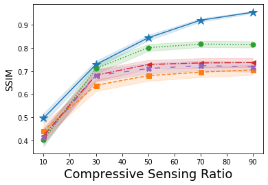
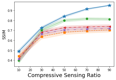
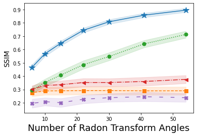
Shown in Fig. 1 is the average SSIM – larger values denote a reconstruction more closely matching the original image – over the reconstructions of one hundred $32\times 32$ images from A-CG-GAN and each of the four comparison methods. Each plot in Fig. 1 gives both the average SSIM and 99% confidence interval – visualized by the background shading – as the dimension of $\bm{y}$ is varied in both CS and CT problems. The underlying DCGAN generator, $\overline{G}$, used for each of these IPs has been trained on 50000 CIFAR10 images. Through a grid search, we set the hyperparameters of A-CG-GAN to be $(\lambda,\mu,\rho)=(0.1,10^{-3},1)$ and $(\lambda,\mu,\rho)=(1,10^{-2},1)$ for CT reconstructions from 60dB and 40dB, respectively. Furthermore, we set $(\lambda,\mu,\rho)=(10^{-6},10^{-6},10^{-4})$ as the hyperparameters of A-CG-GAN for CS reconstructions. Additionally, we use $\widetilde{\Phi}=\Phi=$ discrete cosine transformation and $\widetilde{\Phi}=\Phi=I$ for CS and CT problems, respectively.

In Figs. 1(a), 1(b) and Figs. 1(c), 1(d), CIFAR10 images are reconstructed from CS and CT measurements with an SNR of 60dB and 40dB, respectively. Instead, in Figs. 1(e), 1(f), 1(g), and 1(h), we show the generalizability of our method by reconstructing CalTech101 images, that have been downsampled to size $32\times 32$, while using the same CIFAR10 trained $\overline{G}$.

We observe, from Fig. 1, that A-CG-GAN outperforms, or performs comparably to, each of the four prior art methods in all scenarios. In particular, we highlight that the performance of A-CG-GAN does not saturate as the dimension of $\bm{y}$ increases – i.e., the sampling from the forward measurement mapping increases – while the performance of the comparisons in general does. Additionally, A-CG-GAN is able to generalize well to image distributions outside of the GAN training distribution as shown in Figs. 1(e), 1(f), 1(g), and 1(h).

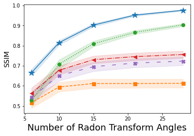
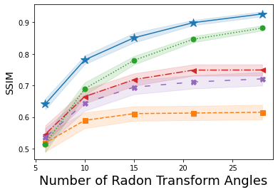
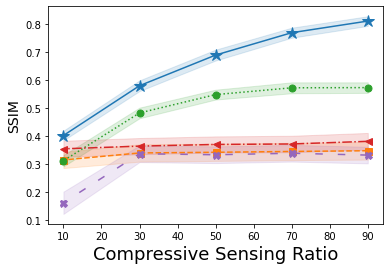
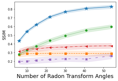
Next, shown in Fig. 2 is the average SSIM over the reconstructions of one hundred $64\times 64$ images from A-CG-GAN and each of the four comparison methods. Each plot in Fig. 2 gives both the average SSIM and 99% confidence interval – visualized by the background shading – as the amount of sampling from the forward measurement mapping – i.e., the dimension of $\bm{y}$ – is varied in both CS and CT problems. The underlying DCGAN generator, $\overline{G}$, used for each of these IPs has been trained on a minimal dataset of roughly 9000 CalTech101 images of size $64\times 64$. Empirically, we choose $(\lambda,\mu,\rho)=0.25\times(10^{-6},10^{-6},10^{-4})$ in A-CG-GAN for CS reconstructions, $(\lambda,\mu,\rho)=(10,0.1,10)$ for 40dB CT reconstructions, and otherwise use the same setup as in the $32\times 32$ image reconstruction cases.

We observe from Fig. 2, that A-CG-GAN outperforms each of the four prior art methods in all scenarios. We highlight, in particular, that while a sub-optimal generator, due to a small training dataset, severely diminished the performance of each of the four comparison methods, A-CG-GAN still provides relatively high-quality reconstructed images as measured by SSIM. This is perhaps anticipated given the dual prior basis our method implements, which alleviates a complete dependence on the generative NN prior as in Bora, Shah, and Latorre [21, 23, 25]. Additionally, we again observe, from Fig. 2, that A-CG-GAN eliminates the performance saturation with increasing sampling from the forward measurement mapping.

Lastly, we remark that Dhar [24] is, in general, the best comparison method to ours as seen in Fig. 1 and Fig. 2. This provides further credence to the benefit of using dual prior information in addition to the GAN prior as Dhar, similar to our dual CG-GAN prior, incorporates a dual sparsity-GAN prior.

Utilizing a dual-structured prior that consists of the powerful CG class of densities and a generative NN, we developed a novel iterative estimate algorithm for linear IPs. Specifically, we proposed an algorithm, called A-CG-GAN, that finds an IP solution satisfying the CG structure of (3) where the scale variable portion of the CG prior is constrained onto the range of a generative NN. Hence, within the informative CG class of distributions, the generative NN captures a rich scale variable statistical representation, which provides a wide, but informative, IP regularization.

We conducted a theoretical analysis on the convergence of A-CG-GAN and showed that, under mild assumptions on the generative NN, a linear rate of convergence is guaranteed up to a neighborhood about a constrained minimizer solution. Subsequently, thorough numerical validation of A-CG-GAN in tomographic imaging and CS IPs was presented. Across multiple datasets and a wide array of forward measurement mappings, we empirically demonstrated that A-CG-GAN outperforms competitive state-of-the-art techniques to IPs that use a GAN prior. Specifically, A-CG-GAN displays three key properties missing from previous techniques using GAN priors for IPs:

1. 1.

   Performance does not saturate with less undersampling from the forward measurement mapping

2. 2.

   Generalization to alternative dataset distributions other than the GAN training distributions is possible

3. 3.

   A sub-optimal generative NN, possibly due to a lack of training data or inadequate training, still provides relatively high-quality reconstructions

Building upon the new foundations established in this paper, we illuminate numerous opportunities for future exploration including: analyzing the performance of A-CG-GAN on larger image reconstructions and on data corrupted by different noise models. Studying each of these objectives can provide greater insight into the practical, real-world applicability of our method.

Another intriguing line of work would be to use a generative NN in A-CG-GAN that has been trained to produce scale variables directly rather than sparsifying an image-generating NN as is done in this paper. We could anticipate a possible improvement in reconstruction performance over the numerical results presented in this paper as the generative NN would directly capture the statistics of the scale variables rather than implicitly capturing these statistics from the overall images.

A last point of future work is to empirically study A-CG-GAN, and each of the four comparisons methods, when the generative NN has been trained on a single category of images. In particular, analyzing image reconstruction performance when the test images are from versus distinct from the training category. The datasets employed in this paper contain images from multiple categories – e.g., CIFAR10 has 10 categories and CalTech101 has 101 categories – creating a significant statistical variability in the datasets, which can result in lower quality images from a generative NN. Instead, when a generative NN is trained on a single category, it is often able to produce higher quality images from this single category. Accordingly, we conjecture that A-CG-GAN would handle the reconstructions of test images distinct from the training category significantly better than the four comparison methods, in much of the same manner that we observed in the $64\times 64$ CalTech101 reconstructions. Furthermore, we conjecture that A-CG-GAN (with $\bm{\mu}_{u}=\bm{1}$) may have minimal improvement, or be matched by, the four comparison methods when test images are sampled from the training category.

In this appendix, we provide mathematical proof details for the main theoretical results of A-CG-GAN, presented in Section III-B, by extending the proof ideas in [25] from ADMM with a single GAN-prior constraint to our case of ADMM with dual-structured CG-GAN-prior constraints.

References

• [1] I. Daubechies, M. Defrise, and C. De Mol, “An Iterative Thresholding Algorithm for Linear Inverse Problems with a Sparsity Constraint,” Commun. Pure Appl. Math, vol. 57, no. 11, pp. 1413–1457, Nov 2004.
• [2] A. Beck and M. Teboulle, “A Fast Iterative Shrinkage-Thresholding Algorithm for Linear Inverse Problems,” SIAM Journal on Imaging Sciences, vol. 2, no. 1, pp. 183–202, Jan 2009.
• [3] S. Ji, Y. Xue, and L. Carin, “Bayesian Compressive Sensing,” IEEE Transactions on Signal Processing, vol. 56, no. 6, pp. 2346–2356, 2008.
• [4] S. Foucart and H. Rauhut, A Mathematical Introduction to Compressive Sensing.   Springer New York, 2013.
• [5] D. Needell and J. A. Tropp, “CoSaMP: Iterative signal recovery from incomplete and inaccurate samples,” Applied and Computational Harmonic Analysis, vol. 26, no. 3, pp. 301–321, May 2009.
• [6] M. J. Wainwright and E. P. Simoncelli, “Scale Mixtures of Gaussians and the Statistics of Natural Images.” in Advances in Neural Information Processing Systems, vol. 12.   MIT Press, 1999, pp. 855–861.
• [7] M. J. Wainwright, E. P. Simoncelli, and A. S. Willsky, “Random Cascades on Wavelet Trees and Their Use in Analyzing and Modeling Natural Images,” Applied and Computational Harmonic Analysis, vol. 11, no. 1, pp. 89–123, 2001.
• [8] C. Lyons, R. G. Raj, and M. Cheney, “A Compound Gaussian Least Squares Algorithm and Unrolled Network for Linear Inverse Problems,” IEEE Transactions on Signal Processing, vol. 71, pp. 4303–4316, 2023.
• [9] C. Lyons, R. G. Raj, and M. Cheney, “Deep Regularized Compound Gaussian Network for Solving Linear Inverse Problems,” IEEE Transactions on Computational Imaging, vol. 10, pp. 399–414, 2024.
• [10] Z. Chance, R. G. Raj, and D. J. Love, “Information-theoretic structure of multistatic radar imaging,” in IEEE RadarCon (RADAR), 2011, pp. 853–858.
• [11] Z. Idriss, R. G. Raj, and R. M. Narayanan, “Waveform Optimization for Multistatic Radar Imaging Using Mutual Information,” IEEE Transactions on Aerospace and Electronics Systems, vol. 57, no. 4, pp. 2410–2425, Aug 2021.
• [12] C. Lyons, R. G. Raj, and M. Cheney, “CG-Net: A Compound Gaussian Prior Based Unrolled Imaging Network,” in 2022 IEEE Asia-Pacific Signal and Information Processing Association Annual Summit and Conference, 2022, pp. 623–629.
• [13] R. G. Raj, “A hierarchical Bayesian-MAP approach to inverse problems in imaging,” Inverse Problems, vol. 32, no. 7, p. 075003, Jul 2016.
• [14] C. Lyons, R. G. Raj, and M. Cheney, “A Deep Compound Gaussian Regularized Unfoled Imaging Network,” in 2022 56th Asilomar Conference on Signals, Systems, and Computers, 2022, pp. 940–947.
• [15] C. Lyons, R. G. Raj, and M. Cheney, “On Generalization Bounds for Deep Compound Gaussian Neural Networks,” arXiv preprint arXiv:2402.13106, 2024, in review by IEEE Transactions on Information Theory.
• [16] K. Gregor and Y. LeCun, “Learning fast approximations of sparse coding,” in Proceedings of the 27th International Conference on Machine Learning, 2010, pp. 399–406.
• [17] J. Song, B. Chen, and J. Zhang, “Deep Memory-Augmented Proximal Unrolling Network for Compressive Sensing,” International Journal of Computer Vision, vol. 131, no. 6, pp. 1477–1496, Jun 2023.
• [18] Y. Su and Q. Lian, “iPiano-Net: Nonconvex optimization inspired multi-scale reconstruction network for compressed sensing,” Signal Processing: Image Communication, vol. 89, p. 115989, 2020.
• [19] J. Adler and O. Öktem, “Learned Primal-Dual Reconstruction,” IEEE Transactions on Medical Imaging, vol. 37, no. 6, pp. 1322–1332, 2018.
• [20] T. Meinhardt, M. Moller, C. Hazirbas, and D. Cremers, “Learning Proximal Operators: Using Denoising Networks for Regularizing Inverse Imaging Problems,” in Proceedings of the IEEE International Conference on Computer Vision, 2017, pp. 1781–1790.
• [21] A. Bora, A. Jalal, E. Price, and A. G. Dimakis, “Compressed Sensing using Generative Models,” in Proceedings of the International Conference on Machine Learning, vol. 70, 2017, pp. 537–546.
• [22] I. Goodfellow, J. Pouget-Abadie, M. Mirza, B. Xu, D. Warde-Farley, S. Ozair, A. Courville, and Y. Bengio, “Generative Adversarial Nets,” in Advances in Neural Information Processing Systems 27 (NIPS 2014), vol. 27, 2014.
• [23] V. Shah and C. Hegde, “Solving Linear Inverse Problems Using GAN Priors: An Algorithm with Provable Guarantees,” in 2018 IEEE International Conference on Acoustics, Speech and Signal Processing (ICASSP), 2018, pp. 4609–4613.
• [24] M. Dhar, A. Grover, and S. Ermon, “Modeling Sparse Deviations for Compressed Sensing using Generative Models,” in Proceedings of the 35th International Conference on Machine Learning, ser. Proceedings of Machine Learning Research, vol. 80.   PMLR, 10–15 Jul 2018, pp. 1214–1223.
• [25] F. Latorre, A. Eftekhari, and V. Cevher, “Fast and Provable ADMM for Learning with Generative Priors,” in Advances in Neural Information Processing Systems (NeurlIPS), vol. 32, 2019.
• [26] G. Song, Z. Fan, and J. Lafferty, “Surfing: Iterative Optimization Over Incrementally Trained Deep Networks,” in Advances in Neural Information Processing Systems (NeurlIPS), vol. 32, 2019.
• [27] A. Jalal, L. Liu, A. G. Dimakis, and C. Caramanis, “Robust Compressed Sensing using Generative Models,” in Advances in Neural Information Processing Systems (NeurlIPS), H. Larochelle, M. Ranzato, R. Hadsell, M. Balcan, and H. Lin, Eds., vol. 33, 2020, pp. 713–727.
• [28] M. Asim, M. Daniels, O. Leong, A. Ahmed, and P. Hand, “Invertible generative models for inverse problems: mitigating representation error and dataset bias,” in International Conference on Machine Learning.   PMLR, 2020, pp. 399–409.
• [29] M. Asim, F. Shamshad, and A. Ahmed, “Blind Image Deconvolution Using Deep Generative Priors,” IEEE Transactions on Computational Imaging, vol. 6, pp. 1493–1506, 2020.
• [30] M. Asim, F. Shamshad, and A. Ahmed, “Solving Bilinear Inverse Problems using Deep Generative Priors,” CoRR, 2018.
• [31] B. Aubin, B. Loureiro, A. Baker, F. Krzakala, and L. Zdeborová, “Exact asymptotics for phase retrieval and compressed sensing with random generative priors,” in Proceedings of The First Mathematical and Scientific Machine Learning Conference, ser. Proceedings of Machine Learning Research, J. Lu and R. Ward, Eds., vol. 107.   PMLR, 20–24 Jul 2020, pp. 55–73.
• [32] P. Hand and B. Joshi, “Global Guarantees for Blind Demodulation with Generative Priors,” Advances in Neural Information Processing Systems (NeurlIPS), vol. 32, 2019.
• [33] P. Hand, O. Leong, and V. Voroninski, “Phase Retrieval Under a Generative Prior,” in Advances in Neural Information Processing Systems (NeurlIPS), S. Bengio, H. Wallach, H. Larochelle, K. Grauman, N. Cesa-Bianchi, and R. Garnett, Eds., vol. 31, 2018.
• [34] G. Jagatap and C. Hegde, “Phase Retrieval using Untrained Neural Network Priors,” in NeurIPS 2019 Workshop on Solving Inverse Problems with Deep Networks, 2019.
• [35] M. Kabkab, P. Samangouei, and R. Chellappa, “Task-Aware Compressed Sensing with Generative Adversarial Networks,” in Proceedings of the AAAI Conference on Artificial Intelligence, vol. 32, 2018.
• [36] D. Ulyanov, A. Vedaldi, and V. Lempitsky, “Deep Image Prior,” in Proceedings of the IEEE Conference on Computer Vision and Pattern Recognition (CVPR), June 2018.
• [37] M. Mardani, E. Gong, J. Y. Cheng, S. S. Vasanawala, G. Zaharchuk, L. Xing, and J. M. Pauly, “Deep Generative Adversarial Neural Networks for Compressive Sensing MRI,” IEEE Transactions on Medical Imaging, vol. 38, no. 1, pp. 167–179, 2019.
• [38] S. Boyd, N. Parikh, E. Chu, B. Peleato, and J. Eckstein, “Distributed Optimization and Statistical Learning via the Alternating Direction Method of Multipliers,” Foundations and Trends® in Machine learning, vol. 3, no. 1, pp. 1–122, 2011.
• [39] D. P. Bertsekas, “On Penalty and Multiplier Methods for Constrained Minimization,” SIAM Journal on Control and Optimization, vol. 14, no. 2, pp. 216–235, 1976.
• [40] S. Boyd and L. Vandenberghe, Convex Optimization.   Cambridge University Press, Mar 2004.
• [41] J. McKay, R. G. Raj, and V. Monga, “Fast stochastic hierarchical Bayesian map for tomographic imaging,” in 51st Asilomar Conference on Signals, Systems, and Computers.   IEEE, Oct 2017, pp. 223–227.
• [42] M. Bertero, C. De Mol, and E. R. Pike, “Linear inverse problems with discrete data: II. Stability and regularisation,” Inverse Problems, vol. 4, no. 3, pp. 573–594, Aug 1988.
• [43] J. Portilla, V. Strela, M. J. Wainwright, and E. P. Simoncelli, “Image Denoising Using Scale Mixtures of Gaussians in the Wavelet Domain,” IEEE Transactions on Image Processing, vol. 12, no. 11, pp. 1338–1351, Nov 2003.
• [44] T. Huang, W. Dong, X. Yuan, J. Wu, and G. Shi, “Deep Gaussian Scale Mixture Prior for Spectral Compressive Imaging,” in Proceedings of the IEEE/CVF Conference on Computer Vision and Pattern Recognition, 2021, pp. 16 216–16 225.
• [45] S. J. Wright, “Coordinate descent algorithms,” Mathematical Programming, vol. 151, no. 1, pp. 3–34, Jun 2015.
• [46] D. P. Kingma and J. L. Ba, “Adam: A Method for Stochastic Optimization,” International Conference on Learning Representations, 2015.
• [47] A. G. Baydin, B. A. Pearlmutter, A. A. Radul, and J. M. Siskind, “Automatic Differentiation in Machine Learning: a Survey,” Journal of Machine Learning Research, vol. 18, 2018.
• [48] M. Abadi, P. Barham, J. Chen, Z. Chen, A. Davis, J. Dean, M. Devin, S. Ghemawat, G. Irving et al., “TensorFlow: A System for Large-Scale Machine Learning,” in 12th USENIX Symposium on Operating Systems Design and Implementation, vol. 16, 2016, pp. 265–283.
• [49] A. Krizhevsky, “Learning Multiple Layers of Features from Tiny Images,” University of Toronto, Tech. Rep., 2009.
• [50] L. Fei-Fei, R. Fergus, and P. Perona, “Learning Generative Visual Models from Few Training Examples: An Incremental Bayesian Approach Tested on 101 Object Categories,” in Conference on Computer Vision and Pattern Recognition Workshop, 2004, pp. 178–178.
• [51] A. Radford, L. Metz, and S. Chintala, “Unsupervised representation learning with deep convolutional generative adversarial networks,” arXiv preprint arXiv:1511.06434, 2015.