eurm10 \checkfontmsam10
Linear stability of slip pipe flow
Abstract
We investigated the linear stability of pipe flow with anisotropic slip length at the wall by considering streamwise and azimuthal slip separately as the limiting cases. Our numerical analysis shows that streamwise slip renders the flow less stable but does not cause instability. The exponential decay rate of the least stable mode appears to be when the Reynolds number is sufficiently large. Azimuthal slip can cause linear instability if the slip length is sufficiently large. The critical Reynolds number can be reduced to a few hundred given large slip lengths. Besides numerical calculations, we present a mathematical proof of the linear stability of the flow to three-dimensional yet streamwise-independent disturbances for arbitrary Reynolds number and slip length, as an alternative to the usual energy analysis. Meanwhile we derived analytical solutions to the eigenvalue and eigenvector, and explained the structure of the spectrum and the dependence of the leading eigenvalue on the slip length. The scaling of the exponential decay rate of streamwise independent modes is shown to be rigorously . Our non-modal analysis shows that overall streamwise slip reduces the non-modal growth and azimuthal slip has the opposite effect. Nevertheless, both slip cases still give the -scaling of the maximum non-modal growth and the most amplified disturbances are still streamwise rolls, which are qualitatively the same as in the no-slip case.
keywords:
1 Introduction
The classic pipe flow with no-slip boundary condition has been proved linearly stable to axisymmetric perturbations (Herron, 1991, 2017), and numerical studies suggest that the flow is linearly stable to any perturbations at arbitrary Reynolds numbers (Meseguer & Trefethen, 2003). The recent work of Chen et al. (2019) presented a rigorous proof of the linear stability of the flow to general perturbations at high Reynolds number regime. Therefore, transition to turbulence in pipe flow is subcritical via finite-amplitude perturbations (see e.g. Eckhardt et al. (2007); Avila et al. (2011)).
However, velocity slip of viscous fluid can occur on super-hydrophobic surfaces (Voronov et al., 2008; Rothstein, 2010), for which slip boundary condition instead of the classic no-slip condition should be adopted for the momentum equations, and the slip boundary condition can potentially influence the stability of the flow. A simplified and widely used slip boundary condition is the Navier slip boundary condition, which has been shown to apply to many flow problems and frequently adopted for linear stability studies (Vinogradova, 1999; Lauga & Cossu, 2005; Min & Kim, 2005; Gan & Wu, 2006; Ren et al., 2008; Ghosh et al., 2014; Seo & Mani, 2016; Chattopadhyay et al., 2017, to list a few). For pipe geometry, although many studies have investigated the linear stability of immiscible and miscible multi-fluid flows with either no-slip or Navier slip boundary condition (Hu & Joseph, 1989; Joseph, 1997; Li & Renardy, 1999; Selvam et al., 2007; Sahu, 2016; Chattopadhyay et al., 2017, etc.), much fewer studies were dedicated to the linear stability of single-phase pipe flow with slip boundary condition. Průša (2009) investigated this problem and showed that, subject to Navier slip boundary condition, pipe flow becomes less stable compared to the no-slip case, however, the destabilization effect is constrained to small Reynolds numbers and is not sufficient to render the flow linearly unstable. Their results indicated that the stability property of pipe flow is not qualitatively affected by the slip boundary condition, regardless of the slip length. For its counterpart in plane geometry, i.e. channel flow, on the contrary, Min & Kim (2005); Lauga & Cossu (2005) reported a stabilizing effect of velocity slip on the linear stability.
Usually, slip length is assumed homogeneous and isotropic, i.e. independent of position and direction at the wall in stability analysis. However, anisotropy in the effective slip length can be incurred by anisotropy in the texture pattern on superhydrophobic surfaces, such as parallel periodic slats, grooves and grates (Lecoq et al., 2004; Bazant & Vinogradova, 2008; Ng & Wang, 2009; Belyaev & Vinogradova, 2010; Asmolov & Vinogradova, 2012; Pralits et al., 2017). For example, Ng & Wang (2009) reported a ratio of down to about 0.25 between the transverse slip length (in the direction perpendicular to the slats) and longitudinal slip length (parallel to the slats). The linear stability of channel flow with anisotropic slip caused by parallel micro-graves was analyzed by Pralits et al. (2017) using the the tensorial formulation of slip boundary condition proposed by Bazant & Vinogradova (2008). Their results showed possibilities of linear instability using special alignment of the micro-graves. Recently, Chai & Song (2019) studied the linear stability of single-phase channel flow subject to anisotropy in slip length by considering streamwise and azimuthal slip separately as the limiting cases, which can potentially be realized or approximated by using specially designed surface texture, e.g. specially aligned micro-grates/graves, according to Bazant & Vinogradova (2008). Their results showed that streamwise slip mainly stabilizes the flow (with increased critical Reynolds number), although it surprisingly destabilizes the flow slightly in a small Reynolds number range, and that azimuthal slip can greatly destabilize the flow and reduce the critical Reynolds number given sufficiently large slip length. The critical Reynolds number can be reduced to a few hundred with a dimensionless azimuthal slip length of , in contrast to for the no-slip case. Their study also indicated that Squire’s theorem (Squire, 1933) ceases to apply when the wall normal velocity and vorticity are coupled via the slip boundary condition, such that the leading instability becomes three dimensional (3-D) rather than two dimensional (2-D) when slip length is sufficiently large, in agreement with Pralits et al. (2017). The stability of 3-D perturbations was not considered by Min & Kim (2005); Lauga & Cossu (2005) in which Squire’s theorem was seemingly assumed.
Differing from channel flow, linear instability is absent at arbitrary Reynolds numbers in classic pipe flow. This raises the question of whether the anisotropy in slip length can also cause linear instability in pipe flow. To our knowledge, this problem has not been studied in pipe geometry. The pseudospectrum analysis of classic pipe flow of Schmid & Henningson (1994); Meseguer & Trefethen (2003) suggests that, despite the linear stability, at sufficiently large Reynolds numbers, a small perturbation to the linear operator associated with the governing equation can possibly change the stability of the system. The slip boundary condition can be thought of as a perturbation to the linear operator with no-slip boundary condition. However, Průša (2009) showed that homogeneous and isotropic slip does not change the spectrum qualitatively no matter how large the slip length (i.e. operator perturbation) is. Following Chai & Song (2019), in this work, we still consider anisotropic slip length in the limiting cases and explore the possibility of linear instability for pipe flow. Aside from the critical Reynolds number as focused on by Chai & Song (2019), here we also investigate the effects of the slip on the spectrum and on the scaling of the leading eigenvalues with Reynolds number. Besides numerical calculations, we also perform analytical studies on the eigenvalues and eigenvectors of the 3-D yet streamwise-independent modes, and discuss about their structure as well as their dependence on the slip length on a theoretical basis, which to our knowledge have not been reported in the literature.
2 Numerical methods
The nondimensional incompressible Navier-Stokes equations read
| (1) |
where denotes velocity and denotes pressure. For pipe geometry, cylindrical coordinates are considered, where , and denote the radial, azimuthal, and streamwise coordinates, respectively. Velocity components , and are normalized by where is the bulk speed (the average of the streamwise velocity on the pipe cross-section), length by pipe radius and time by . The Reynolds number is defined as where is the kinematic viscosity of the fluid. In order to eliminate the pressure and impose the incompressibility condition, we adopt the velocity-vorticity formulation of Schmid & Henningson (1994), with which the governing equations of disturbances reduce to only two equations about the wall normal velocity and wall normal vorticity . With a Fourier-Fourier-Chebyshev collocation discretization, considering perturbations of the form of , the governing equations in the Fourier spectral space read
| (2) |
where
| (3) |
| (4) |
is the scaled time, and unknowns are
| (5) |
The real number is the axial wave number and , which is an integer, is the azimuthal wavenumber. The base flow is denoted as , , and the prime denotes the derivative with respect to . The operators and are defined as and . The other two velocity components and can be calculated as
| (6) |
We use the Robin-type Navier slip boundary condition at the pipe wall for streamwise and azimuthal velocities separately, i.e.
| (7) |
where and are streamwise and azimuthal slip lengths, respectively, and are independent of each other. In spectral space, these boundary conditions apply identically to and given the homogeneity of the slip length. We use the no-penetration condition for the wall-normal velocity component at the wall, i.e. . Lauga & Cossu (2005); Chai & Song (2019) considered the same boundary conditions for slip channel flow. Note that in the isotropic slip case considered by Průša (2009), and are related as , which gives for small slip lengths. With boundary condition (7), given that we impose the same volume flux as in the no-slip case, i.e.
| (8) |
the velocity profile of the constant-volume-flux base flow reads
| (9) |
where represents the unit vector in the streamwise direction. Note that the base flow is independent of . Converting to the system, the boundary condition (7) reads
| (10) |
and
| (11) |
It can be seen that and , i.e. and , are coupled via the slip boundary condition.
In order to avoid the singularity at the pipe center, i.e. , the domain [0, 1] is extended to [-1, 1] and an even number of Chebyshev grid points over [-1, 1] are used such that there is no grid point at . This extension also allows us to use the Chebyshev collocation method for the discretization in the radial direction and the resulted redundancy is circumvented by setting proper parity conditions on and with respect to (Trefethen, 2000; Meseguer & Trefethen, 2003). In this way, no explicit boundary condition is imposed at the pipe center.
To determine whether a mode is linearly stable or not, one only needs to calculate the eigenvalues of the operator and check if any eigenvalue has a positive real part, , which determines the asymptotic growth/decay rate of the corresponding eigenvector as .
3 Streamwise slip
We consider the case of and as the limiting case of streamwise slip being significant and azimuthal slip being negligible.
The effect of the slip on the spectrum is investigated for and is shown in Figure 1 for the modes and . Firstly, panel (a) shows that the eigenvalues of the mode visually all fall on the line ( denotes the imaginary part of the eigenvalue) and in the left half-plane, which suggests that the eigenvalues are all real and negative. Meseguer & Trefethen (2003) reported the same finding for the no-slip case in a large Reynolds number range up to . In fact, the eigenvalues being real and negative can be rigorously proved, see our proof in Section 5.1. Secondly, as increases, it can be observed that there are two groups of eigenvalue, one of which stays constant and the other of which shifts to the right, see the two insets in panel (a). Specifically, as is increased to 0.5, the left eigenvalue in the left inset has moved from the circle to the triangle and finally to the square while the right eigenvalue stays constant. Nontheless, the rightmost eigenvalue increases as increases (see the right inset) which indicates that the flow becomes less stable. In Section 5.2, we will show that the former group corresponds to disturbances with , i.e. and the latter group, on the contrary, is associated with disturbances with , i.e. and, the rightmost eigenvalue belongs to the latter group (see Figure 13).
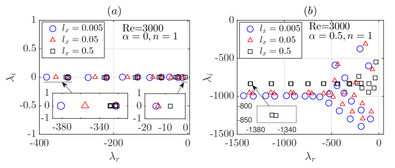
Panel (b) shows the case for the mode . The slip does not qualitatively change the shape of the spectrum. As increases, the eigenvalues overall move to the right. Besides a horizontal shift, there is a shift in the vertical direction either, and meanwhile the spectrum is compressed in the vertical direction, see the comparison between the and the other two cases. Using the term of Schmid & Henningson (1994); Meseguer & Trefethen (2003), the horizontal branch of the spectrum (the part with ) corresponds to mean modes, the upper branch corresponds to wall modes and the lower branch to center modes. Note that the speed of a wave is given by in our formulation. It has been known that the wave speed of the mean modes follows the mean velocity of the ‘two-dimensional’ axial base flow, i.e. in pipe flow (see e.g. Drazin & Reid (1981)), which gives in the no-slip case (Schmid & Henningson, 1994). In our case, the wave speed of the mean modes is decreased by the slip, reducing to 0.5559 for (, see the eigenvalue in Table 1) which is very close to given by with the base flow shown in (9). The wall modes, which are located close to the wall, move at lower speed than the center modes, which are located close to the pipe center and move at speeds close to the centerline velocity. Since we fix the volume flux of the flow while the slip length is varied, the speed of the base flow close to the wall increases as increases, whereas the speed near the pipe center decreases, i.e. the velocity profile becomes flatter, see the base flow given by (9). Therefore, it can be expected that as increases, the speed of the wall-modes increases and that of the center modes decreases, and all three types of modes move at closer speeds. This is exactly what the compression in the vertical direction of the spectrum reveals. The other noticeable effect is that the slip brings the adjacent eigenvalues associated with the mean modes closer as the slip length increases, causing a seemingly degeneracy of the spectrum, see Figure 1(b).
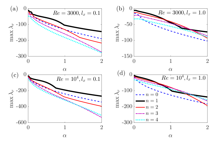
Figure 2 shows the maximum of the real part of the eigenvalue, , as a function of the streamwise wavenumber, , for and . For each , slip lengths and 1.0, and azimuthal wavenumbers , 1, 2, 3 and 4 are considered. The trend shown in the figure suggests that, for both Reynolds numbers, is nearly the least stable mode, i.e. the slowest decaying mode given that all ’s are negative, regardless of the slip length. At small , where is largest, the results suggest that is always the least stable one. At larger , however, is still the least stable when is small, see the case of in panel (a, c), but is not in a range of around , see the case of in panel (b, d). Nevertheless, in this range, is much smaller than that in the small regime. Therefore, as we are most interested in the least stable mode, in the following, we will focus on the modes. In fact, for the modes, we can rigorously prove that is the least stable azimuthal wavenumber, see Appendix B.
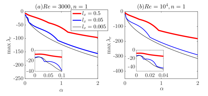
Figure 3 shows as a function of of the modes for (a) and (b). For each , overall increases as increases, i.e. the modes decay more slowly as increases. The insets show the close-up of the small region, in which the dependence of on is not monotonic, with the maximum appears at some small but finite instead of . Nevertheless, the difference between the peak value and the value for is very small, i.e. is nearly the least stable mode, as aforementioned. In fact, the dependence on is not fully monotonic either, see the very small region around for the (the thin black line) and (the blue line) cases as shown in the inset in (a) and around in the inset in (b). However, for and in most range of , our results show a monotonic increase of as increases.
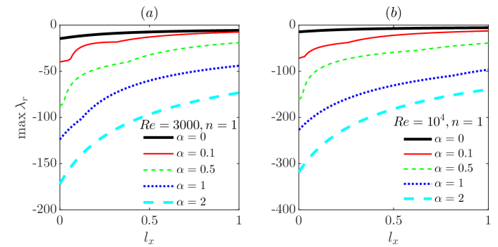
Figure 4 illustrates the dependence of of the modes on in a broader range of . For each , , 0.1, 0.5, 1 and 2 are shown. The trend shows that as keeps increasing, seems to asymptotically approach a plateau with a negative value, i.e. all the modes shown in the figure appear to be linearly stable, for both Reynolds numbers.
The above results suggest that, with streamwise slip, the flow is linearly stable to any perturbations, regardless of the slip length. In order to show evidences in a broader parameter regime, we numerically searched for the global maximum of over and and explored a wider range of up to 10 and of up to . Practically, based on our analysis, we only need to search in a small range of immediately above zero (see the insets in Figure 3) while setting . Specifically, the range of [0, 1.2] is searched at , and the range is decreased as for higher Reynolds numbers. Then we plotted the global maximum of , still denoted as , as a function of , for a few Reynolds numbers ranging from to in Figure 5(a).
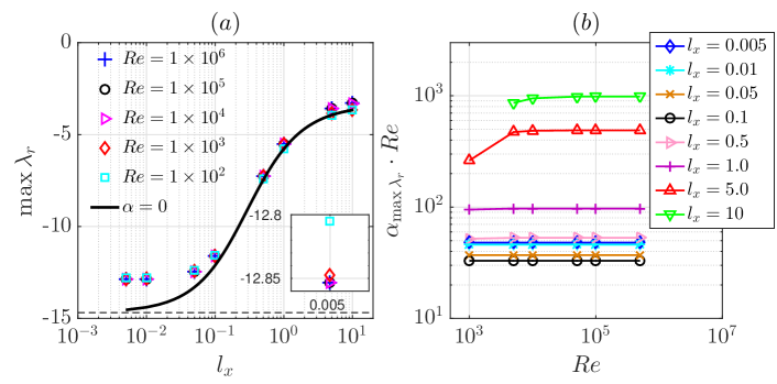
It is interesting to note that our data for high Reynolds numbers all collapse over the whole range investigated, see the cases with above in Figure 5, suggesting that the maximum eigenvalue of the system is independent of . At lower Reynolds numbers, e.g. and in the figure, there is almost a collapse for small () but a small deviation from the high Reynolds number cases can be seen, see the inset that shows the zoom-in at . As increases further, the maximum eigenvalue for and approaches to that of modes, which is strictly -independent (see the proof in Section 5.1). Besides, the figure also shows that the global maximum of is slightly larger than the maximum of the modes over the whole range and the difference is most significant at small . We did not explore further larger considering that the range we investigated is already much larger than the slip length that can be encountered in applications ( in set-ups with characteristic length of one millimeter or larger, because so far the maximum slip length achieved in experiments is micron, see Voronov et al. (2008); Lee et al. (2008); Lee & Jim (2009)). Nevertheless, the -shaped trend as increases suggests that the flow stays stable no matter how large the slip length is. In fact, as , full slip boundary condition is recovered, and the velocity profile of the base flow will be completely flat and no mean shear exists, in which case linear stability can be expected for any perturbations. Panel (b) shows the product of and the at which maximizes globally, denoted as . Interestingly, it seems that this product is a constant when is small () for all the ’s investigated and approaches a constant as is sufficiently high () if . This indicates that scales as for either not very large or in high Reynolds number regime. It should be noted that we observed a non-monotonic dependence of on the slip length, which minimizes at around .
That the global is -independent, as our results suggest, indicates that the slowest exponential decay rate (referred to as decay rate for simplicity hereafter) of perturbations scales as given that the scaled time is used in our formulation, see Eqs. (2). The same scaling was observed by the calculation of Meseguer & Trefethen (2003) for the mode of the classic pipe flow. Therefore, our results suggest that, as , the decay rate of perturbations asymptotically approaches zero and stays negative, i.e. the flow is linearly stable at arbitrary Reynolds number. The -scaling of the slowest decay rate can be rigorously proved for the modes, see Section 5.1.
In a word, in the pure streamwise slip case, we did not observe any linear instability in the large ranges of and that we considered, and based on the data shown in Figure 5, we propose that streamwise slip destabilizes the flow but does not cause linear instability, regardless of the slip length and Reynolds number. A similar destabilizing effect was reported by Průša (2009) for the isotropic slip case.
4 Azimuthal slip
We consider the case of and as the limiting case of azimuthal slip being significant and streamwise slip being negligible.
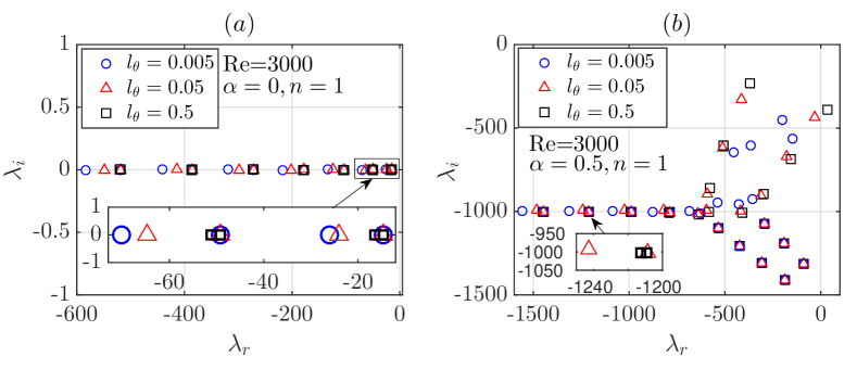
The effect of azimuthal slip on the spectrum is investigated for and is shown in Figure 6 for the modes and . Similar to the streamwise slip case, the eigenvalues of the mode also fall on the line and in the left half-plane, see panel (a). This suggests that the eigenvalues of streamwise-independent modes are all real and negative. We will show a rigorous proof of this observation in Section 5.1. As increases, similar to the streamwise slip case, we also observed two groups of eigenvalues. One group stays constant as the azimuthal slip length changes and the other shifts to the right, see the inset in panel (a). As we will theoretically show in Section 5.2 and 5.3, the former group is associated with the disturbances with and is independent of , and the latter group is associated with the disturbances with . The rightmost eigenvalue belongs to the former group for and can only be overtaken by the latter group if (the two groups precisely overlap when ), i.e. the rightmost eigenvalue can only increase with if . For the and mode, the mean-mode branch overall does not show either a vertical or horizontal shift, but adjacent eigenvalues are brought closer by the increasing slip length, and for there is almost an eigenvalue degeneracy (see the inset in panel (b)). The center-mode branch is nearly unchanged as increases. However, the wall-mode branch is significantly affected. As increases, the wall mode overtakes the center mode and becomes the least stable perturbation, and as is sufficiently large, the rightmost eigenvalue appears in the right half-plane, indicating the onset of a linear instability. In contrast to the streamwise slip case, the wave speed of the mean modes does not change because the speed follows as aforementioned and the base flow is not affected by the azimuthal slip. The speed of the center modes is also not affected, whereas the wave speed of the wall modes is considerably decreased by the slip. This is reasonable because the slip boundary condition should mostly affect the flow close to the wall and should not affect significantly the flow far from the wall.
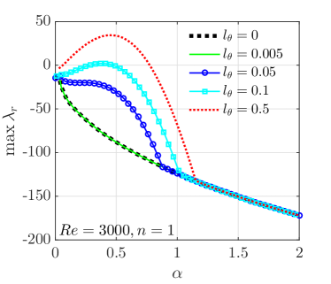
Figure 7 shows maximized over (over [0, 2] in practice), still denoted as , as a function of for , 1, 2, 3 and 4 at . Overall, increases monotonically as increases, while the case seems to stay constant until it starts to increase at around . In the small regime, all modes are linearly stable. As is increased to around 0.1, of the mode becomes positive, indicating a linear instability. As increases further, and 3 also become unstable. In the whole range of investigated, is the least stable/most unstable one, which is also the case for other Reynolds numbers we investigated. Therefore, in the following, we mainly discuss about modes.
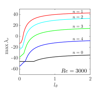
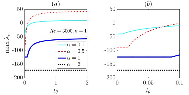
Figure 8 shows of modes , 0.5, 1.0 and 2.0 for and as a function of . The results show that when is small, overall decreases as increases. As is increased, some moderate turns to be the least stable/most unstable mode, see the crossover of (cyan thin line) and 0.5 (red dashed line) cases in the figure. Panel (b) shows the small range, in which it appears that first stays nearly unchanged and then starts to increase, and the trend shows that the larger , the later starts to increase as is increased. The same behavior is also observed for modes and we will show a rigorous proof of this behavior in Section 5.3. Interestingly, the case of seems to stay unchanged up to .
The dependence of on is more comprehensively shown in Figure 9. The smallest shows a monotonic decrease with increasing , which completely collapses onto the curve for , i.e. the classic no-slip case. However, as increases, significantly increases in the region of such that a bump appears in the curves, see those for , 0.1 and 0.5. At certain point, the bump reaches and the flow starts to become linearly unstable if increases further, see the cases of and 0.5. As observed in Figure 8 for the case, the results suggest that of sufficiently large seems unaffected by azimuthal slip in the range investigated, see the collapse of all curves above in Figure 9. It should be noted that as becomes larger, the bump widens up, i.e. is affected by the slip in a wider range of .
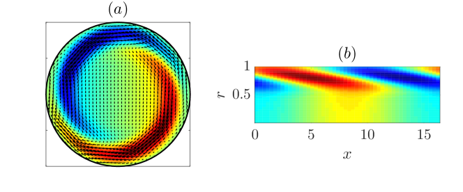
Figure 10 shows the velocity field of the most unstable perturbation of mode for with . Panel (a) shows the in-plane velocity field in the pipe cross-section and (b) shows the pattern of the streamwise velocity in the cross-section. The patterns shown suggest that the flow manifests with a pair of helical waves. The flow structures are mostly located near the wall (), indicating that the most unstable mode is a wall-mode, which can also been seen in Figure 6(b).
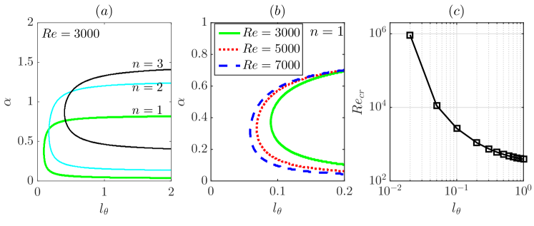
Obviously, azimuthal slip can cause linear instability given sufficiently large slip length. We can search in the - plane to obtain the neutral stability curve for given and . Figure 11(a) shows the neutral stability curves for and , 2 and 3 ( and higher are all stable, see Figure 7). It can be seen that, as increases, the unstable region shifts to the right and upward. However, as the results in Figure 7 show, is the most unstable based on the eigenvalue maximized over and therefore, we only investigate the case in the following. Panel (b) shows the neutral stability curves for and , 5000 and 7000. As increases, the neutral stability curve moves towards the smaller region, indicating that, for a given , the flow becomes more unstable as increases, as expected. The data show that the wavelength of the unstable modes is comparable or significantly larger than the pipe diameter, whereas very long waves () and short waves () are generally stable. That the flow is always stable to perturbations with , regardless of the value of and , can be rigorously proved (see Section 5.1).
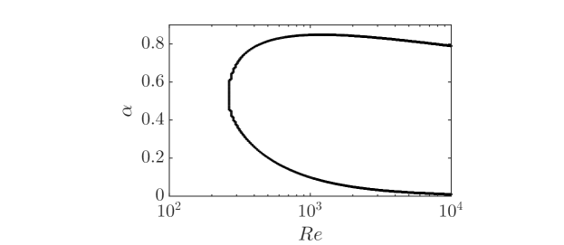
Further, for each , a critical Reynolds number can be determined by searching the first appearance of a positive in the - plane by varying . Figure 11(c) shows as a function of . As shown, is a few hundred if is large (), but the trend suggests that it does not reduce to zero if . Since the classic pipe flow is linearly stable for arbitrary Reynolds number, there is an explosive increase in as decreases, which can be expected because the classic pipe flow will be recovered if . We also explored the limit of , in which case the boundary condition for the azimuthal velocity becomes the full slip condition of
| (12) |
The neutral stability curve for in the plane is shown in Figure 12, which shows that the unstable modes are still long waves with approximately between 0 and 0.8. The critical Reynolds number (the nose of the curve) appears approximately at .
5 Eigenvalues and eigenvectors of streamwise independent modes
We can rigorously prove the linear stability of the base flow to perturbations with . In the following, we do not consider the mode, which should be strictly stable as it is purely dissipative and there can be no energy production mechanism associated with it. In fact, the stability of the classic pipe flow to streamwise independent perturbations has already been proved by Joseph & Hung (1971) using an energy analysis. Nevertheless, here we also account for the effect of the velocity slip and perform analytical studies on the eigenvalues and eigenvectors of modes.
5.1 Proof of linear stability to modes
For , the eigenvalue of the operator satisfies
| (13) |
and
| (14) |
where and compose the eigenvector associated with (see the definition of in (5)). The boundary conditions (10) and (2) reduce to
| (15) |
and
| (16) |
It can be seen that for modes, and are decoupled in the boundary conditions (15) and (16).
We define a space and an inner product associated with this space
| (17) |
where the over-bar represents complex conjugate. Then the operator has the following two properties.
Firstly, for the case of (i.e. the wall normal velocity component ) and , Eqs. (14) becomes
| (24) |
and the operators and are related as . Therefore, Eqs. (24) becomes
| (25) |
Taking the inner product of Eqs. (25) with , we have
| (26) |
According to property (21), given (without streamwise slip) or (with streamwise slip), which leads to , i.e. the eigenvalue is real and negative.
Secondly, we discuss about the case, i.e. the wall normal velocity component . From Eqs. (13), by denoting , we have , i.e.
| (27) |
from which it can be obtained that
| (28) |
where and are constants. Note that for , has to vanish at , because vanishes, and and are finite at . The same applies to . If , , which also vanishes when (using L’Hopital rule). Therefore, and , i.e.
| (29) |
5.1.1 The case without azimuthal slip, i.e.
In case of , the boundary condition (2) or (16) becomes . Taking the inner product (17) of Eqs. (29) and , we have
| (30) |
The second equality in Eqs. (30) holds in spite of that and thus, property (18) cannot be applied directly. Nevertheless, as at in case of , property (18) still holds (this can been seen by taking as and as in Proof 5.1). What follows is that the eigenvalue is real and because and .
5.1.2 The case with azimuthal slip, i.e.
In case of , Eqs. (30) does not hold, except for , because at does not necessarily hold and therefore the second equality in Eqs. (30) does not hold either. For , consider the special case of (if , a rescaling of can easily convert to this special case), Eqs. (29) can be written as
| (31) |
As , Eqs. (31) turns to
| (32) |
Further, the azimuthal slip requires
| (33) |
It follows that, for , has to be zero, otherwise Eqs. (32) and (33) would conflict with each other. That leads to , see Eqs. (30). For , one can solve for from Eqs. (32) and (33) as
| (34) |
which indicates that is real and .
It can be verified that Eqs. (31) has a special solution
| (35) |
and its corresponding homogeneous differential equation is
| (36) |
From the theory of ordinary differential equation, this equation has two linearly independent solutions in . One of the two solutions can be represented as a generalized power series
| (37) |
in which it can be obtained that , and using the standard undetermined coefficient method. Denoting , Eqs. (37) can be written as
| (38) |
The other solution of Eqs. (36) has the following form
| (39) |
However, by L’Hopital rule,
| (40) |
which is unphysical, and therefore should not appear in the general solution of Eqs. (31), i.e. the general solution of Eqs. (31) can be solved as
| (41) |
For simplicity, denoting and using the boundary condition , one can solve for as
| (42) |
consequently,
| (43) |
i.e. satisfies
| (44) |
In the following, we prove that has to be real and given Eqs. (44). For simplicity, let and define as
| (45) |
where is complex. Then, Eqs. (44) states that is a root of the equation . Note that
| (46) |
Then, defining , it can be verified that
| (47) |
in which the prime denotes the derivative with respect to . Further, note that is also a root of Eqs. (44), because the coefficients are all real. That is to say,
| (48) |
where . Then, the difference between Eqs (47) multiplied by and Eqs. (48) multiplied by , integrated along the real axis from 0 to 1 gives that
where the condition is used to derive and . Then we have
| (49) |
Similarly, the sum of Eqs (47) multiplied by and Eqs. (48) multiplied by , integrated along the real axis from 0 to 1 gives that
| (50) |
which indicates because the right hand side is non-zero. Consequently, Eqs. (49) indicates that , i.e. is real.
Subsequently, we can deduce that if because the term in the parentheses and the integral on the right hand side of Eqs. (50) are all positive. In case of , if were positive, one would obtain
| (51) |
and consequently , which would conflict with . Therefore, . Finally, we obtain that for , i.e. for any value of . Since we have shown before that for and for , now we reach the conclusion that is real and for any , regardless of , i.e. the flow is rigorously linearly stable to perturbations with with or without velocity slip.
5.2 Analytical solution of the eigenvalue and eigenvector for modes
We consider the general case with both streamwise and azimuthal slip. For , if , we obtain from Eqs. (44) that satisfies
| (52) |
where Eqs. (34) is used. The Bessel functions of integer order and read
| (53) |
| (54) |
Denoting , i.e. the eigenvalue , it can be observed that is a root of the equation
| (55) |
Next, we show that if . Assuming and , and the boundary condition would give . Recall that the solution to the homogeneous equation Eqs. (36) is
| (56) |
where is a constant. Using the notation of (45), results from (note that if ), which would indicate that the corresponding satisfies . Further, gives
| (57) |
In combination with , we would obtain that
| (58) |
which means that would also be a zero of , i.e. would be a zero of both and . This would conflict with the fact that there exists no comment zero of and . Therefore, and is a root of Eqs. (55) if .
We have proved before that if , which gives . Consequently, gives , which means is a root of , i.e. is also a root of Eqs. (55) (note that the first term disappears if ). Therefore, is a root of Eqs. (55) for any .
For the case of , Eqs. (25) and the corresponding boundary condition (see Eqs. (2) and (15)) imply that the eigenvector has the same form as the solution , and we can deduce that , in which is a root of
| (59) |
For an eigenvalue , the corresponding eigenvector can be solved as
| (60) |
| (61) |
where is a constant and should be determined by the boundary condition Eqs. (15). For an eigenvalue , the eigenvector can be solved as
| (62) |
To sum up, there are always two groups of eigenvalues, corresponding to (given by Eqs. 59) and (given by Eqs. 55), respectively. Particularly, for the no-slip case, Eqs. (55) reduces to and Eqs. (59) reduces to , and it is known that the zeros of and distribute alternately. Therefore, in the no-slip case, these two groups of eigenvalues distribute alternately either. For the streamwise slip case, Eqs. (55) still reduces to , i.e. the eigenvalues do not change with , whereas the eigenvalues will change with . However, there cannot be common roots between and Eqs. 59, otherwise there would be common zeros between and , which conflicts with the fact that there are none common zero between the two. Therefore, as changes, the two groups of eigenvalues distribute in the same alternating pattern as in the no-slip case and there is no over-taking between the two groups, see Figure 1(a) and Figure 13(a). However, this behavior is not guaranteed in the azimuthal slip case as there can be common roots between Eqs. (55) and (59)) given and , i.e. the roots of . Nonetheless, it should be noted that the common roots can only exist at . This implies that, when eigenvalues change with , an over-taking between the two groups may occur at precisely .
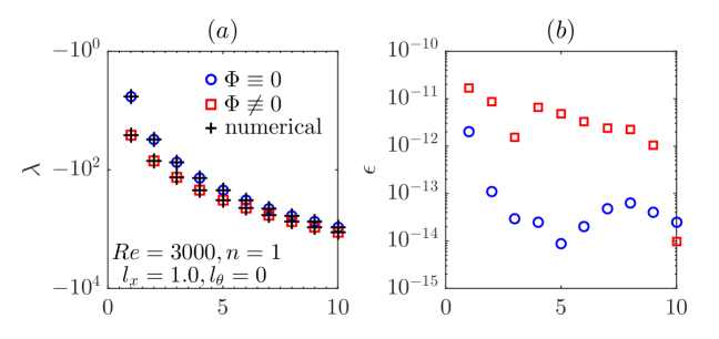
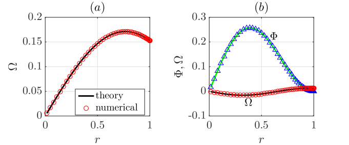
Figure 13 shows the comparison between our analytical solution of the two groups of eigenvalues and numerical calculation for the streamwise slip case of , , and . In panel (a), blue circles are analytical solutions of the first 10 largest eigenvalues given by Eqs. (59), i.e. the corresponding eigenvectors all have , and red squares represent the first 10 largest eigenvalues given by Eqs. (55), i.e. the corresponding eigenvectors all have . Clearly, the leading eigenvalue is and will always be associated with disturbances because no over-taking between the two groups of eigenvalues can occur as varies, as we concluded in Section 5.2. These analytical solutions agree very well with the numerical calculations (the crosses) with relative errors of or lower, see panel (b). The eigenvector associated with the leading eigenvalue (the leftmost circle in Figure 13(a)) is plotted in Figure 14(a). The black line shows the analytical solution given by (62) and the circles show the numerical calculation. The part of the eigenvector is not shown because . Figure 14(b) shows the eigenvector associated with the second largest eigenvalue (the leftmost red square in Figure 13(a)), which has a non-zero part. The figure shows that, for both and , our analytical solutions (lines) agree very well with the numerical calculations (symbols). This comparison validates our theory about the eigenvalue and eigenvector.
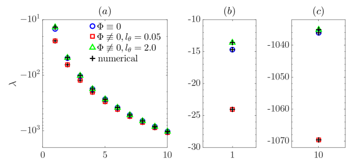
The two groups of eigenvalues of the azimuthal slip cases of and 2.0 for , and are also shown in Figure 15. Again, perfect agreement between the analytical and numerical ones is observed. We can see that, for , the group is entirely below the group, which is independent of , whereas is entirely above the group for , indicating that an over-taking indeed occurs between the two groups as increases. Therefore, for , the leading eigenvalue is associated with disturbances and does not change with (see also Figure 6(a)), whereas it is associated with disturbances and increases with for .
5.3 The dependence of the leading eigenvalue on slip length for modes
Denoting , it can be obtained that, as ,
| (63) |
It can be seen that for , therefore, is positive for sufficiently small . Let be the minimum root of and be the minimum root of . If , it can be derived that
| (64) |
In (5.3), follows from that, at the minimum positive zero of , denoted as , we have because . We showed before that at sufficiently small , therefore, the minimum positive zero of , , should be smaller than given that is continuous with respect to , i.e. , and therefore . Consequently, given , there must be a zero in , i.e. because the function is continuous with respect to . This states that, for the case of , the maximum eigenvalue , denoted as in the following, increases as increases and is independent of . Similarly, one can deduce that the minimum root of Eqs. (59) decreases as increases, consequently, the maximum eigenvalue for the case, denoted as , increases as increases and is independent of .
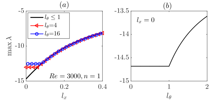
For the special case of , Eqs. (59) becomes and for the case of , Eqs. (55) turns into . Clearly, these two cases share the non-zero roots, i.e. . Therefore, the minimum root of Eqs. (59) is always greater than that of Eqs. (55), i.e. , when . This explains why, for a given , increases monotonically as increases from zero, whereas for a given , first stays constant and only starts to increase until is increased above a threshold, see Figure 16(a). If only azimuthal slip is present, i.e. , firstly stays constant and only starts to increase precisely at , see Figure 16(b). The data shown in the inset of Figure 6(a) also support this conclusion, see that for , 0.05 and 0.5 are identical. It can also be inferred that, given a fixed and that increases with , can only start to increase as increases at some .
In summary, the maximum eigenvalue of modes is an increasing function of or (may not be strictly increasing, depending on the slip length setting, as Figure 16 shows) and is independent of the Reynolds number, which is obvious as does not appear in Eqs. (55) and (59). Nevertheless, the eigenvalues remain negative.
6 Non-modal stability
It has been known that in many shear flows (e.g., pipe, channel and plane-Couette flows), small disturbances can be transiently amplified due to the non-normality of the linearized equations, despite their asymptotic linear stability (Schmid & Henningson, 1994; Meseguer & Trefethen, 2003; Schmid, 2007). This transient amplification is believed to play an important role in the subcritical transition in shear flows. Here, we also investigated the effects of the anisotropic slip on the non-modal stability of the flow. The same method for calculating the transient growth described by Schmid & Henningson (1994) is adopted. The transient growth at time for a mode is defined as
| (65) |
where is the kinetic energy of the perturbation integrated in the whole flow domain at time . For linearly stable flow, will reach the maximum, , at certain time and monotonically decay at larger times. For linearly unstable flow, can be either non-monotonic or monotonic at early stages, depending on the competition between the modal and non-modal growth, and will be dominated by the exponential growth of the most unstable disturbance at large times.
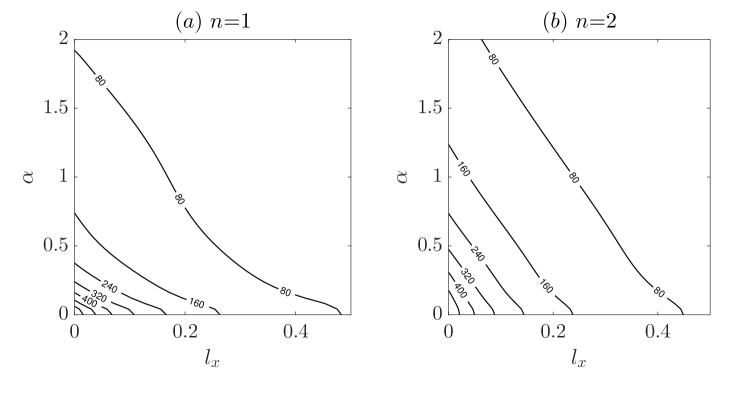
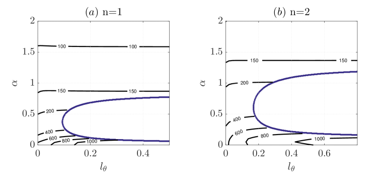
Figure 17 shows at in the - plane () for and (low azimuthal wavenumbers are generally most amplified by non-normality). From the contour lines we can see that steamwise slip reduces and the decrease is monotonic as increases. Intuitively, streamwise slip reduces the background shear such that the lift-up mechanism (Brandt, 2014) is subdued. Therefore, the transient growth should be reduced as our results show. The most amplified mode is still the mode (streamwise rolls) as in the no-slip case (Schmid & Henningson, 1994; Meseguer & Trefethen, 2003).
Figure 18 shows for the azimuthal slip case at in the - plane. Azimuthal wavenumbers and are considered. From the orientation of the contour lines we can see that azimuthal slip increases . Presumably, azimuthal slip can enhance streamwise vortices because it reduces wall friction and allows finite azimuthal velocity at the wall, and therefore, the lift-up mechanism can be enhanced exhibiting increased transient growth as our results show. For , in the range investigated, the most amplified mode is still the mode as in the no-slip case. However, for , as increases, the most amplified mode is no longer the streamwise independent one but one with a small finite streamwise wavenumber (long wavelength), see panel (b). For example, the most amplified mode is approximately for above about 0.1. Similar behavior has also been reported for channel flow (Chai & Song, 2019). The two bold lines in the figure enclose the linearly unstable regions in which is theoretically infinite, therefore, the linearly unstable region is left blank. Unlike the streamwise slip case where the slip length significantly reduces the transient growth throughout the and ranges investigated (see Figure 17), azimuthal slip only significantly affects the transient growth for small and nearly does not affect that of larger , see the nearly horizontal contour lines for relatively large . Besides, even for small , quickly saturates as increases. To sum up, azimuthal slip only affects the transient growth of the modes with small streamwise wavenumbers and the effect saturates as the slip length increases.
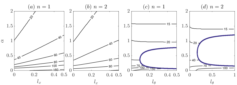
Figure 19 shows the time instant when is reached, , for the cases shown in Figure 17 and 18. In the streamwise slip case (panel (a,b)), for both and 2, the slip increases and the effect is more significant for larger . In the azimuthal slip case (panel (c,d)), for small (), is also slightly increased by the slip, whereas for larger , is slightly decreased by the slip, in contrast to the streamwise slip case. Overall, for the modes with small , i.e. most amplified modes due to non-normality, both streamwise and azimuthal slip only mildly increase .
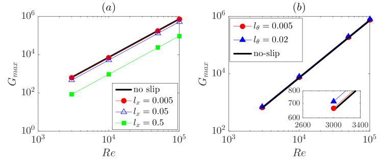
In the no-slip case, the global (maximized over and ) is known to scale as when is large (Meseguer & Trefethen, 2003). In the presence of streamwise and azimuthal slip, the scaling is also investigated and shown in Figure 20. In the streamwise slip case (panel (a)), the lines for , 0.05 and 0.5 appear to be parallel to the no-slip case with a downward vertical shift, suggesting a -scaling for any streamwise slip length. Similarly, for azimuthal slip, the scaling also seem to be . For this case, we only investigated and 0.02 in the linearly stable regime because larger will cause linear instability.
7 Conclusions and discussions
It has been well established that the classic pipe flow is (asymptotically) linearly stable. In this paper, we studied the effect of velocity slip on the linear stability of pipe flow. Our results show that the leading eigenvalue increases with streamwise slip length but remains negative, i.e. streamwise slip renders the flow less stable but does not cause linear instability, similar to the effect of isotropic slip length on the flow (Průša, 2009). Interestingly, our results suggest that the leading eigenvalue is independent of , or equivalently, the slowest decay rate of disturbances scales as (note that time is scaled by in our formulation). It should be pointed out that this scaling holds at sufficiently high Reynolds numbers (). For relatively low Reynolds numbers (100 and 1000 in our study), there is a very slight deviation from the scaling for and the deviation is substantial at larger . The -scaling of the decay rate is the same as what was observed for the mode of the classic pipe flow by Meseguer & Trefethen (2003). Besides, our results show that the streamwise wavenumber at which the eigenvalue maximizes is not but also scales as . However, if is very large (, and note that in applications the slip length is generally much smaller), the eigenvalue maximizes at at relatively low Reynolds numbers (100 and 1000 in our study) and this scaling also only holds at high Reynolds numbers ().
This destabilizing effect appears to be opposite to the stabilizing effect of streamwise slip reported for channel flow (the stabilizing effect is mainly observed for 2-D perturbations) (Lauga & Cossu, 2005; Min & Kim, 2005; Chai & Song, 2019). Here, we only provide a possible explanation for the least stable/most unstable perturbation (referred to as the leading perturbation for simplicity) of the two flows. We speculate that the different flow structures of the leading perturbations of the two flows are responsible. For pipe flow, we proved that the component of the leading perturbation for modes vanishes. The globally leading perturbation has very small (), which indicates that should be nearly vanishing. Therefore, the production rate of kinetic energy () should be also very small and the decay rate of disturbances should be dominated by the dissipation rate. Intuitively, velocity slip reduces the dissipation rate due to the reduced wall friction, therefore, the decay rate of the least stable perturbation decreases, i.e. the flow appears to be destabilized. In contrast, for channel flow, the leading perturbations are 2-D Tollmien-Schlichting waves for small slip length, which have a substantial wall-normal velocity component (comparable to the streamwise component). Therefore, the kinetic energy production is significant and even dominant in the variation of the kinetic energy. Streamwise slip reduces the base shear () and therefore subdues the production. If the reduction in the production rate outweighs the decrease in the energy dissipation rate due to the reduced wall friction, the flow will be stabilized. This is probably why stabilizing effect of the streamwise slip on channel flow was observed.
On the contrary, azimuthal slip, given sufficiently large slip length, causes linear instability, similar to the finding of Chai & Song (2019) for channel flow. Our results show that azimuthal slip destabilizes helical waves with wavelengths considerably larger than the pipe diameter, whereas it does not affect the stability of waves with much shorter wavelengths and in the long wavelength limit, i.e. . The critical Reynolds number decreases sharply as increases and gradually levels off at around a few hundred as and at approximately 260 as . Similar destabilizing effect was reported for channel flow (Chai & Song, 2019). Azimuthal slip serves as an example for a perturbation to the linear operator associated with the linearized Navier-Stokes equations with no-slip boundary condition that destabilizes the originally stable system.
Regarding the stability of the classic pipe flow to streamwise independent perturbations, using an energy analysis, Joseph & Hung (1971) concluded the absolute and global stability of the flow, i.e. the flow is asymptotically (as ) stable to such perturbations with arbitrary amplitude. Here, for the linear case and from a mathematical point of view, we rigorously proved that the eigenvalues of streamwise independent modes () are real and negative, for arbitrary slip length and arbitrary Reynolds number. Besides, the eigenvalue of the modes is proved to be strictly independent of Reynolds number in our formulation, in agreement with the numerical calculation by Meseguer & Trefethen (2003). We derived analytical solutions to the eigenvalue and eigenvector for modes and verified our theory by numerical calculations. We also proved that, the eigenvalues of modes consist of two groups: One group is associated with disturbances with , i.e. , and the other is associated with disturbances with , i.e. (see Fig 13 and Figure 15). The two groups distribute alternately. For the streamwise slip case, the latter group stays constant while the former group changes with . It is the other way round for the azimuthal slip case. Interestingly, for the streamwise slip case, the leading eigenvalue belongs to the group and does not switch group as changes, whereas for the azimuthal slip case, it switches from the group to the group as crosses 1.0 from below (see Figure 15). When both and are non-zero, dominates the leading eigenvalue if . If , the leading eigenvalue first stays constant and can only start to increase at a threshold as increases (see Figure 16). Such analytical solutions might inspire asymptotic analysis in the limit of small streamwise wavenumber.
Non-modal analysis shows that streamwise slip greatly reduces the transient growth, whereas azimuthal slip significantly increases the transient growth for disturbances with very small steamwise wavenumbers but nearly does not affect that for disturbances with larger streamwise wavenumbers, aside from the linear instability caused by the slip. Both streamwise slip and azimuthal slip give the -scaling of the maximum transient growth, the same as in the no-slip case (Schmid & Henningson, 1994; Meseguer & Trefethen, 2003). Similar effects were observed for channel flow (Chai & Song, 2019).
Linear instability caused by anisotropic slip at low Reynolds numbers is of interest for small flow systems, such as microfluidics, in which the Reynolds number is usually low but the non-dimensional slip length can be significantly large using advanced surface texturing techniques. The instability can be exploited to enhance mixing or heat transfer in applications involving small flow systems. Larger non-modal growth caused by azimuthal slip can potentially cause earlier subcritical transition to turbulence. Besides, introducing modal instability into originally sub-critical flows may also help to better understand the transition mechanism in such flows.
8 Acknowledgements
The authors acknowledge financial support from the National Natural Science Foundation of China under grant number 91852105 and 91752113 and from Tianjin University under grant number 2018XRX-0027. The comments from the reviewers are also highly appreciated.
9 Declaration of interests
The authors report no conflict of interest.
Appendix A Numerics
Firstly, we briefly explain the implementation of the boundary condition (10) and (2) in the eigenvalue problem for the linear system (2).
The eigenvalue equation reads
| (66) |
where is the unknown vector composed of and , see (5). Boundary conditions (10) and (2) couple and , unlike in the no-slip case. In our Fourier-Fourier-Chebyshev collocation discretization, is a vector and the operator is discretized as a matrix, where is the number of collocation grid point on the radius. Adopting the Chebyshev differentiation matrix of Trefethen (2000) which is of spectral accuracy, the matrix is dense and the radial differentiation of at a single grid point is calculated using the value of at all collocation points on the radius. Given that is known at , i.e. at , the size of the system can be reduced by one. The boundary conditions (10) and (2) give two linear algebraic equations about and at the collocation points, from which we can further eliminate two unknowns. By doing so, the system size is reduced by 3, i.e. to , from which the eigenvalue problem can be solved with the boundary conditions being taken accounted for.
Secondly, we show the convergence test of our numerical calculation. We consider the case of , and , as presented in Figure 1(b) and Figure 6(b). We change the number of Chebyshev points and check the convergence of the mean-mode, wall-mode and center-mode separately. Table 1, 2 and 3 shows the resolutions and the eigenvalue of an arbitrarily selected mean mode and the rightmost eigenvalues corresponding to the wall- and center-mode. It can be seen that grid numbers , 64 and 128 give very close values of the eigenvalues, which differ only after about 7 digits after the decimal point (the relative difference is ), for all the slip length of 0.005, 0.05, 0.5 and the case of . The convergence test show that, for the calculation of the rightmost eigenvalues and for calculating the mean mode at , 32 points are sufficient. Solely for calculating the rightmost eigenvalue, we used 32 points for , 1000 and 10000, and 64 points for and . We checked the convergence by doubling the number of grid points and found these numbers sufficient. It should be noted that, although 32 points are sufficient for calculating both of the rightmost eigenvalue and the spectrum at , more grid points may be needed for accurately calculating the spectrum than for calculating the rightmost eigenvalue at higher Reynolds numbers (Trefethen, 2000; Meseguer & Trefethen, 2003).
, , , and mean-mode wall-mode 32 -622.180970763082-1006.803438258427 -106.901701568167-600.000309196652 64 -622.180970617437-1006.803438460110 -106.901701568129-600.000309195248 128 -622.180970549502-1006.803438403115 -106.901701574121-600.000309193566 center-mode 32 -87.144443682906-1299.140360156589 64 -87.144443682943-1299.140360156482 128 -87.144443681739-1299.140360155874 , , , and mean-mode wall-mode 32 -530.922788817816-953.518793751342 -68.522846170133-646.557599422173 64 -530.922788815748-953.518793737632 -68.522846166147-646.557599425783 128 -530.922788808102-953.518793754673 -68.522846166147-646.557599425783i center-mode 32 -80.309678415026-1203.366029301252 64 -80.309678415070-1203.366029301237 128 -80.309678413737-1203.366029300673
, , , and mean-mode wall-mode 32 -582.2041335894776-833.8681859837275 -32.3669400581618-546.6565442837639 64 -582.2041335893674-833.8681859850334 -32.3669400570418-546.6565442835596 128 -582.2041336044291-833.8681859835294 -32.3669400643051-546.6565442852506 center-mode 32 -36.8382964038017-757.7599724649968 64 -36.8382964035955-757.7599724652722 128 -36.8382963977050-757.7599724664044
, , , and mean-mode wall-mode 32 -878.143428857252-1000.225260064803 -147.212095816072-565.187041064729 64 -878.143429638119-1000.225258436485 -147.212095816866-565.187041057138 128 -878.143429646590-1000.225258451813 -147.212095817673-565.187041057973 center-mode 32 -88.016026669448-1311.995868654545 64 -88.016026669520-1311.995868654469 128 -88.016026668333-1311.995868653794 , , , and mean-mode wall-mode 32 -818.018362966476-992.813175584590 -30.701258513947-434.347551571943 64 -818.018361688704-992.813172416195 -30.701258511491-434.347551570607 128 -818.018361708603-992.813172372158 -30.701258513706-434.347551572422 center-mode 32 -88.015855528115-1312.001178576785 64 -88.015855528186-1312.001178576701 128 -88.015855526922-1312.001178575825
, , , and mean-mode wall-mode 32 -794.161410360041-1006.311883474201 33.866513836957-391.619593748286 64 -794.161408826090-1006.311880389063 33.866513839707-391.619593747032 128 -794.161408715927-1006.311880293383 33.866513840046-391.619593749138 center-mode 32 -88.013747237500-1312.003625793072 64 -88.013747237549-1312.003625792987 128 -88.013747236338-1312.003625792171
, , , and mean-mode wall-mode 32 -637.771735030362-1019.911762553870 45.558397965700-383.081240915272 64 -637.771735090255-1019.911762536828 45.558397968779-383.081240913500 128 -637.771735157437-1019.911762419706 45.558397965363-383.081240919212 center-mode 32 -88.013312066798-1312.003902287461 64 -88.013312066887-1312.003902287400 128 -88.013312039270-1312.003902226469
Appendix B The dependence of the leading eigenvalue on the azimuthal wavenumber for
Our numerical calculations in Section 3 and 4 showed that modes are the least stable/most unstable modes. Here we show the dependence of of modes on the azimuthal wavenumber and prove that is indeed the least stable azimuthal mode. For this purpose, we only need to prove that the minimum non-zero roots of Eqs. (55) and (59) all increase with .
Note that the root of Eqs. (55) is independent of . Because the zeros of and distribute alternately, it can be easily seen that, if , the minimum positive root of Eqs. (55) is located between the minimum positive zeros of and . Therefore, the minimum positive root of Eqs. (55) increases with because the positive zeros of and all increase with , i.e., decreases as increases if .
If , we need to prove that the minimum positive root of
| (67) |
is smaller than that of , i.e. Eqs. (55). We already showed in Eqs. (63) that at sufficiently small , i.e. for sufficiently small . Denoting the minimum positive root of Eqs. (55) as , we only need to show that . Using the property of Bessel function of
| (68) |
and Eqs. (55), can be rewritten as
| (69) |
It is easily seen that , therefore, we need to show that
| (70) |
or equivalently,
| (71) |
in order to prove that , given . Noticing that if , we can prove if we can show that .
In Section 5.3 we proved that the minimum positive root of Eqs. (55) decreases as increases, therefore, is minimized at . To prove that for any , we only need to show that holds for , with which Eqs. (55) reduces to . That at sufficiently small indicates that at sufficiently small given . Therefore, requires that , i.e. for any . In fact, we can show that if such that has to satisfy . Using the series form of Bessel function, means
| (72) |
Because of the absolute convergence of the two infinite series in Eqs. (72), we only need to show that for any positive even number ,
| (73) |
if . Rearranging Eqs. (B), we have
| (74) |
which obviously holds because . To sum up, we have proved that if , therefore, , which satisfies , must satisfy . Consequently, Eqs. (71) and hold, and thusly the minimum positive root of Eqs. (67) is smaller than , which indicates that the minimum positive root of Eqs. (55) increases with , i.e. decreases with .
Next, we prove that the minimum positive root of Eqs. (59) also increases with . The equation
| (75) |
share the non-zero roots with Eqs. (59), therefore, we only need to prove the same statement for Eqs. (75). Denoting the minimum positive zero of as , we next show that monotonically increases in such that there is no positive root of Eqs. (75) in , i.e. the minimum positive root of Eqs. (75) increases with . Using the property of Bessel function of , where ‘′’ denotes the derivative with respect to , we take the derivative of with respect to and obtain
| (76) |
It is easy to see that is positive at sufficiently small (the derivation is similar to that of being positive at sufficiently small , see Eqs. (63)), consequently, in . As is smaller than the minimum positive zero of , we have in . Therefore, in , i.e. monotonically increases and there is no positive root of Eqs. (75) in . In other words, the minimum positive root of is always larger than that of , i.e. the minimum positive root of Eqs. (59) increases with , and therefore decreases with . Now, we reach the conclusion that decreases with for modes because and both decrease with .
References
- Asmolov & Vinogradova (2012) Asmolov, E. S. & Vinogradova, O. I. 2012 Effective slip boundary conditions for arbitrary one-dimensional surfaces. J. Fluid Mech. 706, 108–117.
- Avila et al. (2011) Avila, K., Moxey, D., De Lozar, A., Avila, M., Barkley, D. & Hof, B. 2011 The onset of turbulence in pipe flow. Science 333, 192–196.
- Bazant & Vinogradova (2008) Bazant, M. Z. & Vinogradova, O. I. 2008 Tensorial hydrodynamic slip. J. Fluid Mech. 613, 125–134.
- Belyaev & Vinogradova (2010) Belyaev, A. V. & Vinogradova, O. I. 2010 Effective slip in pressure-driven flow past super-hydrophobic stripes. J. Fluid Mech. 652, 489–499.
- Brandt (2014) Brandt, L. 2014 The lift-up effect: the linear mechanism behind transition and turbulence in shear flows. Eur. J. Mech. B/Fluids 47, 80–96.
- Chai & Song (2019) Chai, C. & Song, B. 2019 Stability of slip channel flow revisited. Phys. Fluids 31, 084105.
- Chattopadhyay et al. (2017) Chattopadhyay, G., Usha, R. & Sahu, K. C. 2017 Core-annular miscible two-fluid flow in a slippery pipe: A stability analysis. Phys. Fluids 29, 097106.
- Chen et al. (2019) Chen, Q., Wei, D. & Zhang, Z. 2019 Linear stability of pipe Poiseuille flow at high Reynolds number regime. arXiv:1910.14245v1 [math.AP] .
- Drazin & Reid (1981) Drazin, P. G. A. & Reid, W. H. 1981 Hydrodynamic Stability. Cambridge University Press.
- Eckhardt et al. (2007) Eckhardt, B., Schneider, T. M., Hof, B. & Westerweel, J. 2007 Turbulence transition in pipe flow. Annu. Rev. Fluid Mech. 39, 447–68.
- Gan & Wu (2006) Gan, C.-J. & Wu, Z.-N. 2006 Short-wave instability due to wall slip and numerical observation of wall-slip instability for microchannel flows. J. Fluid Mech. 550, 289–306.
- Ghosh et al. (2014) Ghosh, S., Usha, R. & Sahu, K. C. 2014 Linear stability analysis of miscible two-fluid flow in a channel with velocity slip at the walls. Phys. Fluids 26, 014107.
- Herron (1991) Herron, I. H. 1991 Observations on the role of vorticity in the stability theory of wall bounded flows. STUDIES IN APPLIED MATHEMATICS 85, 269–286.
- Herron (2017) Herron, I. H. 2017 A unified solution of several classical hydrodynamic stability problems. QUARTERLY OF APPLIED MATHEMATICS LXXVI, 1–17.
- Hu & Joseph (1989) Hu, H. H. & Joseph, D. D. 1989 Lubricated pipelining : stability of core-annular flow. part 2. J. Fluid Mech. 205, 359–396.
- Joseph (1997) Joseph, D. D. 1997 Core-annular flows. Annu. Rev. Fluid Mech. 29, 65–90.
- Joseph & Hung (1971) Joseph, D. D. & Hung, W. 1971 Contributions to the nonlinear theory of stability of viscous flow in pipes and between rotating cylinders. Arch. Rational Mech. Anal. 44, 1–22.
- Lauga & Cossu (2005) Lauga, E. & Cossu, C. 2005 A note on the stability of slip channel flows. Phys. Fluids 17, 088106.
- Lecoq et al. (2004) Lecoq, N., Anthore, R., Cichocki, B., Szymczak, P. & Feuillebois, F. 2004 Drag force on a sphere moving towards a corrugated wall. J. Fluid Mech. 513, 247–264.
- Lee et al. (2008) Lee, C., Choi, C.-H. & Jim, C.-J 2008 Structured surfaces for a giant liquid slip. Phys. Rev. Lett. 101, 064501.
- Lee & Jim (2009) Lee, C. & Jim, C.-J 2009 Maximizing the giant liquid slip on superhydrophobic microstructures by nanostructuring their sidewalls. Langmuir 25, 12812.
- Li & Renardy (1999) Li, Jie & Renardy, Yuriko 1999 Direct simulation of unsteady axisymmetric core–annular flow with high viscosity ratio. J. Fluid Mech. 391, 123–149.
- Meseguer & Trefethen (2003) Meseguer, A. & Trefethen, L.N. 2003 Linearized pipe flow to Reynolds number . J. Comput. Phys. 186, 178–197.
- Min & Kim (2005) Min, T. & Kim, J. 2005 Effects of hydrophobic surface on stability and transition. Phys. Fluids 17, 108106.
- Ng & Wang (2009) Ng, C.-O. & Wang, C. Y. 2009 Stokes shear flow over a grating: Implications for superhydrophobic slip. Phys. Fluids 21, 013602.
- Pralits et al. (2017) Pralits, J. O., Alinovi, E. & Bottaro, A. 2017 Stability of the flow in a plane microchannel with one or two superhydrophobic walls. PHYSICAL REVIEW FLUIDS 2, 013901.
- Průša (2009) Průša, V. 2009 On the influence of boundary condition on stability of Hagen-Poiseuille flow. Computers and Mathematics with Applications 57, 763–771.
- Ren et al. (2008) Ren, L., Chen, J.-G. & Zhu, K.-Q. 2008 Dule role of wall slip on linear stability of plane Poiseuille flow. Chin. Phys. Lett. 26, 601–603.
- Rothstein (2010) Rothstein, J. P. 2010 Slip on superhydrophobic surfaces. Annu. Rev. Fluid Mech. 42, 89–109.
- Sahu (2016) Sahu, K. C. 2016 Double-diffusive instability in core–annular pipe flow. J. Fluid Mech. 789, 830–855.
- Schmid (2007) Schmid, P. J 2007 Nonmodal stability theory. Ann. Rev. Fluid Mech. 39, 129–162.
- Schmid & Henningson (1994) Schmid, P. J & Henningson, D. S. 1994 Optimal energy density growth in hagen-poiseuille flow. J. Fluid Mech. 277, 197–225.
- Selvam et al. (2007) Selvam, B., Merk, S., Govindarajan, R. & Meiburg, E. 2007 Stability of miscible core-annular flows with viscoisity stratification. J. Fluid Mech. 592, 23–49.
- Seo & Mani (2016) Seo, J. & Mani, A. 2016 On the scaling of the slip velocity in turbulent flows over superhydrophobic surfaces. Phys. Fluids 28, 025110.
- Squire (1933) Squire, H. B. 1933 On the stability of three dimensional disturbances of viscous flow between parallel walls. Proc. Roy. Soc. A 142, 621–638.
- Trefethen (2000) Trefethen, L. N. 2000 Spectral methods in Matlab. SIAM.
- Vinogradova (1999) Vinogradova, O. I. 1999 Slippage of water over hydrophobic surfaces. Int. J. Min. Process 56, 31–60.
- Voronov et al. (2008) Voronov, R. S., Papavassiliou, D. V. & Lee, L. L. 2008 Review of fluid slip over superhy-drophobic surfaces and its dependence on the contact angle. Industr. Eng. Chem. Res. 47, 2455–2477.