Local condensation of charge-$4e$ superconductivity at a nematic domain wall

Shortly after the development of the BCS model for superconductivity, it was recognized that a gas of bosons could also form a coherent state of pairs of bosons before the Bose-Einstein condensation of individual particles, provided that strong enough attractive interactions are present [1, 2]. In condensed matter systems, pair condensation of bosonic quasiparticles has been studied in various settings, from biexcitons in semiconductors [3, 4] to two-magnon bound states in frustrated magnets [5, 6]. A fascinating possibility is the emergence, in superconducting materials, of a coherent state of pairs of Cooper pairs, dubbed quartets [7, 8, 9, 10, 11, 12]. Theoretically, a charge-$4e$ superconducting state is expected to display gapless excitations [13, 14] and half flux-quantum vortices [10]. Experimentally, charge-$4e$ bound states have been recently invoked to explain puzzling magneto-transport data in kagome superconductors [15, 16].

In the case of bosonic particles, the state with paired bosons is thermodynamically stable only when there is more than one bosonic “flavor” available for condensation (e.g. spin-1 bosons) [17]. This suggests that “multi-flavor” superconductors are a promising setting to search for charge-$4e$ superconductivity. Indeed, theoretical proposals for quartet formation have included spin-3/2 systems [18], spinor condensates [19], multi-band superconductors [20], pair-density waves [10, 21, 22, 23, 24, 25, 26, 27], and multi-component superconductors [28, 29, 30, 31, 32, 33]. In the latter case, the superconductor is described by multiple gap functions related by lattice symmetries, $\boldsymbol{\Delta}=\left(\Delta_{1},\,\Delta_{2},\cdots\right)$; in group-theory jargon, $\boldsymbol{\Delta}$ transforms as a multi-dimensional irreducible representation (IR) of the point group. A broad range of pairing states belong to this category, including several versions of $p$-wave and $d$-wave states in tetragonal, hexagonal, and cubic lattices [34, 35]. More importantly, there is experimental evidence for the realization of multi-component pairing in various systems of interest, from heavy-fermions [36, 37, 38] to moiré superlattices [39] to doped topological insulators [40, 41, 42].

Charge-$4e$ order emerges in multi-component superconductors via the condensation of a complex-valued composite order parameter $\left\langle\boldsymbol{\Delta}\cdot\boldsymbol{\Delta}\right\rangle\neq 0$ (distinct from the real-valued composite $\left\langle\boldsymbol{\Delta}^{\dagger}\cdot\boldsymbol{\Delta}\right\rangle$), while the superconducting order parameter itself remains zero, $\left\langle\boldsymbol{\Delta}\right\rangle=0$, such that the transition temperature of the composite order, $T_{4e}$, is larger than the superconducting one, $T_{c}$ [28, 43]. This spontaneous symmetry-breaking, which is driven by fluctuations and thus not captured by mean-field approaches, lowers the $U(1)$ gauge symmetry to $Z_{2}$; the latter is further broken if $\left\langle\boldsymbol{\Delta}\right\rangle$ becomes non-zero. It is said then that the charge-$4e$ and charge-$2e$ superconducting states are intertwined, and that the former is a vestigial order of the latter [44, 45].

The main obstacle for the stabilization of charge-$4e$ vestigial order is the competition with other vestigial phases, most notably nematic and ferromagnetic. Indeed, besides $U(1)$ symmetry, the ground state of a multi-component superconductor also breaks either time-reversal (chiral superconductor) or rotational symmetry (nematic superconductor) [46]. These additional symmetries can be broken before the onset of superconductivity via the condensation of real-valued composite order parameters. Large-$N$ and variational calculations found that the corresponding vestigial nematic and ferromagnetic orders generally preempt the onset of charge-$4e$ order [47, 48] – except for the special case of a hexagonal nematic superconductor [28].

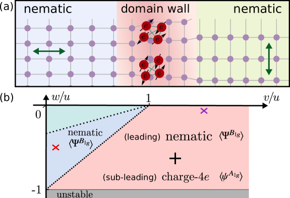
In this work, we investigate whether the local suppression of the leading nematic or ferromagnetic vestigial order enables the local condensation of charge-$4e$ order. As a motivation, we first discuss a 2D triplet superconductor without spin-orbit coupling (SOC), whose multi-component gap function has a continuous SU(2) symmetry. In this case, the continuous symmetry globally forbids quasi-long-range order of any composite order parameter, except for charge-$4e$. We then study the more realistic situation of discrete multi-component superconductors in tetragonal and hexagonal systems. While long-range order in the competing vestigial channel is unavoidable, it is locally suppressed due to the formation of domains. Focusing on a nematic superconductor on the tetragonal lattice, we employ a real-space variational approach that treats all composite orders on an equal footing. We find a wide range of parameters for which charge-$4e$ order is condensed at the nematic domain walls while the superconducting order parameter remains uncondensed, as illustrated schematically in Fig. 1(a). We finish by discussing the experimental manifestations of this local condensation and candidate materials.

To set the stage, we discuss a special case in which, for symmetry reasons alone, the only order that can be stabilized is charge-$4e$. Consider a 2D system in which the electrons experience negligible SOC (e.g. graphene) and, in addition to spin, have another pseudospin degree of freedom (e.g. sublattice or valley). Enforcing the pairing state to be momentum-independent and pseudospin-singlet, the gap function must be spin-triplet and represented by an order parameter $\boldsymbol{\Delta}=(\Delta_{1},\,\Delta_{2},\,\Delta_{3})^{T}$ that transforms as a vector in SU(2) spin space. This is nothing but the $\boldsymbol{d}$-vector of a triplet superconductor [34, 35], albeit even in momentum. While there is no indication of valley-singlet spin-triplet superconductivity in graphene, this type of state has been studied in twisted moiré systems [49, 50, 51, 52] and Bernal bilayer graphene [32, 53]. The superconducting action is given by

with (bare) superconducting susceptibility $\chi_{\mathsf{q}}^{-1}$ and $\mathsf{q}=\left(\mathbf{q},\omega_{n}\right)$ denoting momentum and Matsubara frequency. The interaction part has Landau coefficients $u$ and $v$, where $\mathsf{x}=\left(\mathbf{x},\tau\right)$ denotes position and imaginary time. The mean-field phase diagram of this model is well-established [54, 55], displaying different types of unitary and non-unitary pairing depending on the sign of $v$.

To describe the vestigial orders, however, it is necessary to go beyond mean-field [45]; for our purposes, a group-theoretical analysis is sufficient. There are four symmetry-breaking bilinear combinations of $\boldsymbol{\Delta}$: two real-valued composites $\boldsymbol{\Psi}^{(l=1)}=\mathsf{i}\boldsymbol{\Delta}\times\bar{\boldsymbol{\Delta}}$ and $\Psi_{\mu\nu}^{(l=2)}=\frac{1}{2}\left(\Delta_{\mu}\bar{\Delta}_{\nu}+\Delta_{\nu}\bar{\Delta}_{\mu}\right)-\frac{1}{3}\,\delta_{\mu\nu}\left|\boldsymbol{\Delta}\right|^{2}$ and two complex-valued ones, $\psi^{(l=0)}=\boldsymbol{\Delta}\cdot\boldsymbol{\Delta}$ and $\psi_{\mu\nu}^{(l=2)}=\Delta_{\mu}\Delta_{\nu}-\frac{1}{3}\,\delta_{\mu\nu}\left(\boldsymbol{\Delta}\cdot\boldsymbol{\Delta}\right)$, where $\bar{z}\equiv z^{*}$. The superscript indicates the transformation properties in SU(2) spin-space, corresponding to a scalar ($l=0$), a vector ($l=1$), or a tensor ($l=2$). Each composite has a clear physical interpretation: $\boldsymbol{\Psi}^{(l=1)}$ corresponds to time-reversal symmetry-breaking and, thus, vestigial ferromagnetic order. $\Psi_{\mu\nu}^{(l=2)}$ is associated with rotational symmetry-breaking in spin-space, and therefore denotes (spin-)nematic vestigial order [56, 57, 31]. Finally, $\psi^{(l=0)}$ and $\psi_{\mu\nu}^{(l=2)}$ correspond to $s$-wave and $d$-wave charge-$4e$ vestigial orders, respectively.

Because $\boldsymbol{\Psi}^{(l=1)}$, $\Psi_{\mu\nu}^{(l=2)}$, $\psi_{\mu\nu}^{(l=2)}$, and $\boldsymbol{\Delta}\equiv\boldsymbol{\Delta}^{(l=1)}$ itself transform non-trivially in SU(2) spin-space (i.e. they are at least Heisenberg-type order parameters), none of them can sustain (quasi-)long-range order at non-zero temperatures in 2D. On the other hand, because $\psi^{(l=0)}$ is a complex scalar (i.e. XY-type), it can establish quasi-long-range order through a BKT transition. Therefore, the only state allowed to develop quasi-long-range order in this model is the vestigial charge-$4e$ phase. We note that similar 2D and 1D models for triplet superconductors [31, 32, 33] and spinor condensates [19] have been previously studied and shown to support charge-$4e$ order.

Despite illuminating, the simple model above is not representative of realistic multi-component superconductors, where either SOC is not negligible or singlet states are realized. Yet, it highlights an efficient strategy to realize charge-$4e$ order: suppression of the other, leading, vestigial phases. While this generally cannot be accomplished globally via Mermin-Wagner’s theorem, vestigial nematic or ferromagnetic states tend to form domains to minimize the elastic or magnetic dipolar energies. To explore this idea, we consider a generic two-component superconducting order parameter $\boldsymbol{\Delta}=(\Delta_{1},\Delta_{2})$, which could describe $(p_{x},p_{y})$-wave or $(d_{xz},d_{yz})$-wave states in tetragonal and hexagonal lattices [34, 35], or $(d_{x^{2}-y^{2}},d_{xy})$-wave pairing in hexagonal systems and $45^{\circ}$-twisted bilayer tetragonal $d$-wave superconductors [58]. In contrast to the previous example, $\boldsymbol{\Delta}$ now transforms as a two-dimensional IR of a discrete point group. While we will focus on tetragonal ($\mathrm{D_{4h}}$) superconductors, where $\boldsymbol{\Delta}$ transforms as the IR $E_{g}$ or $E_{u}$, the conclusions apply to all other cases.

We start by classifying all possible composite order parameters. As shown in [43], seven different bilinear combinations can be formed. Apart from the symmetry-preserving bilinear $\Psi^{A_{1g}}=\boldsymbol{\Delta}^{\dagger}\tau^{0}\boldsymbol{\Delta}$, with Pauli matrices $\tau^{i}$ acting on the $\boldsymbol{\Delta}$ subspace, there are three additional real-valued bilinears:

Here, $\Psi^{A_{2g}}$ breaks time-reversal-symmetry and causes ferromagnetism, while $\Psi^{B_{1g}}$ and $\Psi^{B_{2g}}$ break tetragonal symmetry and cause nematicity. The three complex-valued bilinears are given by

and describe, respectively, $s$-wave, $d_{x^{2}-y^{2}}$-wave, and $d_{xy}$-wave charge-$4e$ superconductivity. In our notation, $\Psi^{n}$ ($\psi^{n}$) denotes real-valued (complex-valued) bilinears, whereas the superscript $n$ indicates the IR according to which the composite transforms. The superconducting action is $\mathcal{S}=\int_{\mathsf{x}}r_{0}\left|\boldsymbol{\Delta}_{\mathsf{x}}\right|^{2}+\;\mathcal{S}^{\mathrm{grad}}\;+\;\mathcal{S}^{\mathrm{int}}\,,$ where $r_{0}=a_{0}(T-T_{0})$ denotes the bare SC transition ($a_{0},T_{0}>0$) and $\mathcal{S}^{\mathrm{grad}}$ contains the symmetry-allowed gradient terms [35]. The interaction part is given by [43]

and contains three independent interaction parameters $u>0$ and $v,w>-u$. The mean-field phase diagram in the $\left(\frac{v}{u},\,\frac{w}{u}\right)$ parameter space is well-established, displaying chiral and two types of nematic superconductivity [35, 10, 46].

The vestigial orders associated with each mean-field ground state were analyzed in Ref. [43] via a variational approach. The leading vestigial instability is always that of a real-valued composite (nematic or ferromagnetic) whereas the vestigial charge-$4e$ orders are always subleading. While our conclusions hold across the entire phase diagram, hereafter we focus on the $v>0>w$ region [Fig. 1(b)], where the superconducting ground state is nematic and the competing vestigial phases are $d_{x^{2}-y^{2}}$ nematic ($\Psi^{B_{1g}}$) and $s$-wave charge-$4e$ ($\psi^{A_{1g}}$). In bulk, the only vestigial order realized is the nematic one [43]. However, because the effective interaction in the charge-$4e$ channel is attractive, the system could gain energy by condensing this mode in regions where nematic order is suppressed. Due to its Ising-like character, $\Psi^{B_{1g}}$ can sustain long-range order at non-zero temperatures. However, because of the linear coupling between $\Psi^{B_{1g}}$ and strain, nematic domains must form to minimize the elastic energy and accommodate long-range lattice deformations. This opens up the possibility of $\psi^{A_{1g}}$ condensation at nematic domain walls.

To proceed, we employ a real-space Gaussian variational approach, which treats all vestigial channels equally, on a 1D grid of length $L$ and $i=1,\dots,N$ sites. The variational ansatz consists of a trial action $\mathcal{S}_{0}$ [59, 60, 61, 43], which in our case is $\mathcal{S}_{0}=\frac{1}{2}\frac{L}{T}\sum_{i}\hat{\boldsymbol{\Delta}}_{i}^{\dagger}\,G_{i}^{-1}\,\hat{\boldsymbol{\Delta}}_{i}+\mathcal{S}^{\mathrm{grad}}$. Represented in the Nambu basis $\hat{\boldsymbol{\Delta}}_{i}=(\boldsymbol{\Delta}_{i},\bar{\boldsymbol{\Delta}}_{i})$, the local inverse Green’s function

contains the real-valued ($\Phi_{i}^{n}$) and complex-valued $(\phi_{i}^{n},\bar{\phi}_{i}^{n})$ variational parameters, and the mass renormalization parameter $R_{i}=r_{0}+\Phi_{i}^{A_{1g}}$. Because $\mathcal{S}_{0}$ is Gaussian, it is straightforward to compute the variational free energy

where $Z_{0}=\int D(\boldsymbol{\Delta},\bar{\boldsymbol{\Delta}})\,e^{-\mathcal{S}_{0}}$ is the partition function of the trial action. The detailed evaluation of Eq. (6) is shown in the Supplementary Material (SM). Importantly, the original Landau coefficients $u$, $v$, and $w$ appear in $F_{v}$ as different combinations in each symmetry channel, corresponding to effective interactions $U_{A_{1g}}=3u+v+w$, $U_{A_{2g}}=u+3v-w,$ $U_{B_{1g}}=u-v+3w$, $U_{B_{2g}}=u-v-w$, $u_{A_{1g}}=u-v+w$, $u_{B_{1g}}=u+v+w$, and $u_{B_{2g}}=u+v-w$ [43]. An attractive interaction ($U_{n},u_{n}<0$) indicates a potential instability, signaled by the condensation of the corresponding variational order parameter ($\Phi_{i}^{n},\,\phi_{i}^{n}$). Importantly, a vestigial phase only emerges if superconductivity is not immediately triggered by $\Phi_{i}^{n},\,\phi_{i}^{n}\neq 0$. In the variational approach, this condition can be verified by confirming that the variational superconducting susceptibility $\chi$, which is given by a combination of $R_{i}$, $\Phi_{i}^{n}$, and $\phi_{i}^{n}$ (see SM for details), remains finite.

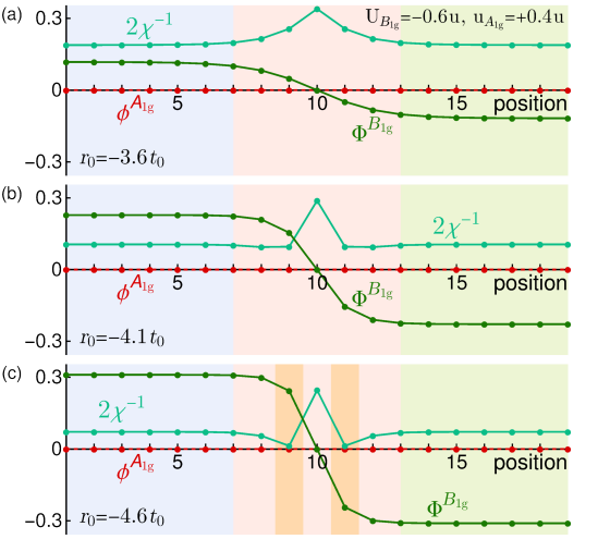
In bulk, for most of the $\left(\frac{v}{u},\,\frac{w}{u}\right)$ phase diagram, there are two competing attractive vestigial-order channels, corresponding to a real-valued composite (nematic/ferromagnetic) and a complex-valued one ($s$-wave/$d$-wave charge-$4e$). As demonstrated in Ref. [43], the nematic/ferromagnetic instability is always the leading one in bulk [Fig. 1(b)]. Our goal is to determine the fate of these phases along a nematic domain wall. We therefore numerically minimize the free energy (6) for the $N$-site 1D grid with domain-wall boundary conditions $\Phi_{1}^{B_{1g}}=-\Phi_{N}^{B_{1g}}=\Phi_{0}^{B_{1g}}$, where $\Phi_{0}^{B_{1g}}$ is the (self-consistently obtained) bulk value of the nematic order parameter (see SM for additional details). Consider first the phase diagram region where the only attractive vestigial-order channel is the nematic, i.e. $U_{B_{1g}}<0$ but $u_{A_{1g}}>0$ [red cross in Fig. 1(b)]. The results are shown in Fig. 2. As the control parameter $r_{0}\propto T-T_{0}$ is decreased, a nematic domain emerges below a temperature that coincides with the bulk nematic critical temperature. As expected, the domain wall becomes sharper as the temperature is lowered, since the wall width scales as $t_{0}/|\Phi_{0}^{B_{1g}}|$ where $t_{0}$ is the gradient-term stiffness. At the domain-wall center, the superconducting susceptibility $\chi$ is suppressed, consistent with the fact that vestigial order enhances the superconducting transition. Interestingly, $\chi^{-1}$ has a non-monotonic spatial dependence, displaying a dip at the domain-wall boundaries, which can lead to local condensation of superconductivity [yellow region of Fig. 2(c)]. No sign of charge-$4e$ order is observed, consistent with a repulsive effective interaction in this channel.

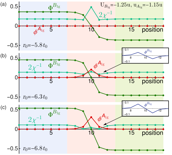
Consider now the phase-diagram region where the charge-$4e$ vestigial channel is attractive, but subleading to the nematic, $U_{B_{1g}}<u_{A_{1g}}<0$ [purple cross in Fig. 1(b)] . As shown in Fig. 3, upon decreasing $r_{0}$, nematic order emerges first, in two domains. However, in contrast to Fig. 2, the charge-$4e$ order parameter $\phi^{A_{1g}}$ condenses inside the domain wall while the superconducting susceptibility $\chi$ remains finite. This is the main result of the paper. Because the domain wall is one-dimensional, this should be understood as a local condensation, since phase slips will destroy long-range order along the wall. Note, even though the $d$-wave charge-$4e$ channel is repulsive in this phase-diagram region, the order parameter $\phi^{B_{1g}}$ condenses due to the trilinear coupling between $\Phi^{B_{1g}}$, $\phi^{A_{1g}}$, and $\bar{\phi}^{B_{1g}}$ (see the inset) [43]. We verified that this behavior is not particular to this set of parameters, but occurs in any region of the $\left(\frac{v}{u},\,\frac{w}{u}\right)$ phase diagram where $s$-wave/$d$-wave vestigial charge-$4e$ order is sufficiently attractive but subleading to nematic/ferromagnetic vestigial order.

In this work, we employed a variational approach to demonstrate that charge-$4e$ order locally condenses at nematic domain walls that emerge in the normal-state of nematic superconductors upon approaching the superconducting transition. Before the onset of superconductivity, the system is unstable towards the formation of vestigial nematic and charge-$4e$ orders arising from the fluctuation-induced condensation of composite superconducting order parameters. Because nematic order generally wins over charge-$4e$ order, the suppression of nematic order along the domain wall enables the system to further minimize the free energy by condensing charge-$4e$ order. Since an analogous mechanism also applies for chiral superconductors, our results point to a wide class of systems – multi-component superconductors – where local charge-$4e$ order can potentially emerge. Among the materials for which there is strong experimental evidence for nematic superconductivity, doped $\mathrm{Bi_{2}Se_{3}}$ [62, 40, 42, 41] and twisted bilayer graphene (TBG) [39, 63, 64] are the most promising candidates to display this effect. Indeed, a vestigial nematic phase exists in doped $\mathrm{Bi_{2}Se_{3}}$ [65, 66], whereas in TBG, normal-state nematic order appears close to the superconducting dome [39]. There are also several chiral-superconductor candidates [67], including the widely studied heavy-fermion UPt₃ [36, 37, 38].

An important question is how to experimentally detect this effect. Since charge-$4e$ order emerges at nematic domain walls, local probes such as scanning tunneling microscopy (STM) and scanning near-field optical microscopy (SNOM) are ideal. Because the charge-$4e$ state is expected to be gapless [13, 14], its density-of-states (DOS) profile, which can be accessed in a standard STM measurement, will likely differ from the normal-state DOS only in subtle ways. On the other hand, Josephson-STM, in which a superconducting tip is used [68, 69], could provide more direct evidence for quartets. The SNOM technique has the unique capability of probing the local optical response with a few nanometers resolution, from which the properties of the local optical conductivity $\sigma(\omega,\boldsymbol{r})$ can be inferred [70, 71]. Because the charge-$4e$ state has a non-zero superfluid density [14], $\mathrm{Im}\,\sigma(\omega,\boldsymbol{r})\sim 1/\omega$ is expected to emerge at low frequencies near nematic domain walls. While this behavior could also be due to a charge-$2e$ superconducting filament, only in the charge-$4e$ case this behavior would be accompanied by a gapless DOS, which can be probed via STM. These results also reveal the tantalizing possibility of using uniaxial strain to control the charge-$4e$ phase, since beyond a critical strain value, the sample becomes mono-nematic-domain and local charge-$4e$ order disappears.