Local Element Operations for Curved Simplex Meshes
Abstract
Mesh optimization procedures are generally a combination of node smoothing and discrete operations which affect a small number of elements to improve the quality of the overall mesh. These procedures are useful as a post-processing step in mesh generation procedures and in applications such as fluid simulations with severely deforming domains. In order to perform high-order mesh optimization, these ingredients must also be extended to high-order (curved) meshes. In this work, we present a method to perform local element operations on curved meshes. The mesh operations discussed in this work are edge/face swaps, edge collapses, and edge splitting (more generally refinement) for triangular and tetrahedral meshes. These local operations are performed by first identifying the patch of elements which contain the edge/face being acted on, performing the operation as a “straight-sided one” by placing the high-order nodes via an isoparametric mapping from the master element, and smoothing the high-order nodes on the elements in the patch by minimizing a Jacobian-based high-order mesh distortion measure. Since the initial “straight-sided guess” from the placement of the nodes via the isoparametric mapping frequently results in invalid elements, the distortion measure must be regularized which allows for mesh untangling for the optimization to succeed. We present several examples in 2D and 3D to demonstrate these local operations and how they can be combined with a high-order node smoothing procedure to maintain mesh quality when faced with severe deformations.
keywords:
high-order; curved mesh; mesh optimization; edge flip; edge collapse; deforming domains120XX4023
A. Shi and P.-O PerssonLocal Element Operations for Curved Simplex Meshes
A. Shi, Department of Mathematics, University of California, Berkeley, Berkeley, CA 94720-3840, U.S.A. (andrewshi@math.berkeley.edu)
… \norevised \noaccepted
1 INTRODUCTION
High-order methods have received considerable interest in the computational science community in the last two decades. This is due to their potential to deliver highly accurate solutions at a comparable cost to traditional low-order methods. In fact, for certain classes of problems — such as turbulent flow — it is widely believed that high-order methods will be required for accurate and grid-converged solutions [1]. Much of the great promise of high-order methods is due their ability to handle complex geometries with unstructured meshes. These methods require high-order (curved) meshes to ensure the curved geometry is represented with sufficient accuracy to enable the high-order convergence rate of these methods. However, the existence (or rather, lack thereof) of robust and automated high-order mesh generation procedures is still one of the main bottlenecks in the widespread adoption of these methods in the design process. To this end, the high-order community has identified high-order mesh generation as a topic deserving of considerable research attention and as one of the top pacing items in high-order method research [2, 3]. One might say curved meshing first distinguished itself as a distinct research topic within mesh generation in 2015, the first year it had its own dedicated session at the International Meshing Roundtable [4]. In terms of available software, Gmsh is a widely used free software with the capability to generate and display curved meshes for elements of arbitrarily high-order [5]. Up until fairly recently, there were no commercial high-order mesh generators available before Pointwise released support for this in 2019 [6]. We refer the reader to the introduction of [7] for a recent survey of the current state of affairs of high-order meshing research and additional references.
Most straight sided mesh generation procedures proceed in two steps: 1) the initial creation of a mesh from geometry through a method like advancing front, Delaunay or octree, and 2) a mesh optimization post-processing step to improve element quality. There is a large body of literature on these mesh quality improvement procedures. While those works may differ in their notions of optimality and specific techniques used, they largely agree mesh optimization via node movement and discrete, localized element operations are the best way to perform mesh quality improvement. Freitag and Ollivier-Gooch [8] consider various node smoothing procedures and face and edge swapping operations, and show that each mechanism fails to significantly improve the mesh quality when used individually but result in very high quality meshes when combined. They offer a variety of empirical recommendations on how to do so and demonstrate the effectiveness of their schedules on a variety of tetrahedral mesh geometries. De Cougny and Shephard [9] combine edge collapses and splitting operations for the purpose of mesh adaptation. Klinger and Shewchuk [10] consider a richer set of operations in an effort to take these ideas to an extreme to find the highest quality mesh, assuming that speed is not the highest priority. We refer the reader to Section 3 of their paper where they survey many of the commonly (as well as lesser used) discrete mesh operations. These are some of the “classic” papers in the field for mesh quality improvement for linear meshes, and while the focus of this paper is on curved meshes, the field of linear mesh quality improvement is still highly active. Some more recent contributions include, but are certainly not limited to directions like new discrete operations to reach better local minima [11, 12], and the inclusion of parallelization [13, 14, 15].
Now the question is how to extend these ideas to curved meshes. Existing work [16, 17, 18, 19] on high-order node smoothing primarily takes the approach of optimization-based minimization of some energy functional or objective function that quantifies high-order mesh distortion. The key issues here are the need for mesh distortion metrics for high-order elements [20, 21] and a procedure for high-order untangling [19, 22, 23]. In principle, some of the approaches to curved mesh generation such as the solution of a linear/nonlinear elasticity analogy [24, 25, 26, 27] or a PDE-based approach [28] could also be adapted for the purpose of high-order mesh smoothing. There is practically no literature on the use of local element operations for curved meshes. To the best of the authors’ knowledge, the only existing work on high-order mesh operations [29] considers face and edge swaps for tetrahedral meshes with second-order () elements.
It is clear that further developments in these areas will be required to advance the current state of curved mesh generation and adaptivity. The difficulty of directly acting on high-order meshes is one possible explanation for why nearly all curved mesh generation approaches are of the a priori variety rather than direct methods [30] which proceed in the same two phases as most straight-sided mesh generators do. In the context of finite element solutions, solution quality is frequently dictated by the mesh element of the worst quality. Local mesh operations for curved meshes could be an inexpensive and direct way to deal with this and other applications such as the repair of deforming high-order domains occurring in time-dependent fluid simulations.

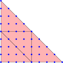
The main goal of this paper is to answer the question, “How we can extend local element operations for straight-sided meshes (Figure 1) to high-order triangular and tetrahedral meshes?” One key difference from the low-order case is that there are many valid ways to perform these operations due to the additional degrees of freedom afforded by the high-order nodes (Figure 2). So there is now an optimal way to perform these local operations by placing these additional nodes in a way to minimize a high-order Jacobian-based mesh distortion measure. In particular, this paper will discuss high-order face and edge swaps, edge collapses and edge splitting for triangular and tetrahedral meshes. The remainder of this article is organized as follows. In Section 2, we introduce the high-order Jacobian based distortion measure and its untangling capabilities. In Section 3, we describe the process of performing these operations, and discuss some practical details related to their implementation. In Section 4, we present multiple examples illustrating how these operations can be combined with high-order node smoothing to repair curved meshes that undergo severe deformations. Finally, in Section 5, we offer concluding remarks and directions for future research.

2 DISTORTION MEASURE AND UNTANGLING
We describe the construction of the high-order distortion measure used in this work for node smoothing from a standard linear distortion measure, which is then regularized to allow for simultaneous smoothing and untangling [31, 32]. We also offer some comments on how this measure is used in our setting for optimization.
2.1 High-order distortion measure
We introduce the distortion measure for linear elements (2). This measure – known as the inverse mean-ratio shape measure – was first introduced in [33, 34]. This measure is widely used in the meshing community as a shape distortion metric due to its many desirable properties such as the standard invariance to translation, rotation, and scaling, but is also special as a geometric shape measure that also enjoys many of the desirable properties of an algebraic mesh quality metric [35]. In particular, this measure is shown to be convex [36] and well-suited for optimization.
As an aside, we note the metric we are about to introduce is geometric in nature, as are most metrics in use today, as opposed to being PDE or solution based. In the course of using mesh generation and adaptation in the numerical solution of PDEs, we point out that using a metric that is geometric in nature may not perfectly align with the ultimate goal of solving the PDE since the metric employed was not based on the PDE solution. This is addressed in [37] where the author discusses the notion of “bridging the gap between a priori quality metrics and solution-dependent metrics”.


Consider a linear element having the desired shape and size (the ideal element) and a corresponding element in physical space . From these we can define a unique affine mapping . It is frequently convenient to introduce the notion of the master element and define two additional mappings (Figure 3a) that map from the master element to the ideal and physical element, respectively. We can define in terms of the these mappings as follows
| (1) |
The element shape distortion metric is defined as
| (2) |
where is the spatial dimension, is the Frobenius norm, and . Note that for linear elements, since is affine, its Jacobian is constant. This distortion measure quantifies the deviation of the shape of the physical element with respect to the ideal element . This distortion measure is 1 for the ideal element and tends to infinity as the physical element degenerates. It is often convenient to define a corresponding quality measure as
| (3) |
For high-order elements, we can no longer apply (2) directly because the mapping is no longer affine, so is no longer constant. Roca et al. describes an extension of the linear distortion measure to high order triangular [20] and tetrahedral [21] elements. The idea is that since the linear measure quantifies the local deviation between the ideal and physical elements, we can obtain a high-order element-wise distortion measure by integrating the linear measure on the physical high order element
| (4) |
where is the area of the physical element and in this work. Explicit expressions for the isoparametric mappings for the high-order case (Figure 3b) in terms of shape functions are given in [20].
2.2 Regularization and untangling
The distortion measure needs to be modified to eliminate the singularity so an optimization procedure can recover from an invalid initial configuration. We use the regularization procedure introduced independently by [31, 32] around the same time, but follow the notation [32] which replaces in the denominator of (2) by
| (5) |
where is a positive element-wise parameter. This regularized Jacobian is a monotonically increasing function of such that , which tends to 0 when tends to , which allows us to overcome the vertical asymptote at in the original measure. This parameter is only set for a non-zero value if there exists an invalid element in the mesh under consideration, otherwise it is set to zero for a mesh with all valid elements. Using the regularized Jacobian, we can now modify (2) to obtain a linear distortion measure capable of simultaneous smoothing and untangling
| (6) |
and use this to define a high-order regularized measure analogous to (4). Figures 5 and 6 of [19] provide a useful illustration of how this regularized distortion metric compares to the original for a simple example.
What remains is the issue of how to pick this positive elementwise regularization parameter . We certainly require the original () and regularized () distortion measures to have nearby minima, so needs to be sufficiently small. On the other hand, has to be large enough to ensure that is significant compared to in the expression for . When this idea was originally introduced in [32], this parameter was chosen in a fairly ad hoc manner by testing a few values for a given initial tangled mesh. In [19], a heuristic was developed to choose a constant value of for each element. Their setting deals with high-order mesh generation by curving the boundaries of a well-shaped straight-sided mesh and minimizing the regularized distortion metric. For them, in the mapping , each physical element in the curved mesh has the ideal element as the corresponding element in the original straight-sided mesh. They propose to choose this parameter solely based off information from the straight-sided ideal element. Defining and imposing
| (7) |
for some given tolerance implies
| (8) |
They argue that should be small compared to and select , giving the final value for as
The value is observed to work well in practice and accomplish the tradeoff required on the value of (Figure 4). Our setting deals with high-order mesh smoothing, so we choose the ideal element to always be the equilateral triangle/tetrahedron. For the unregularized distortion measure, the actual size of is irrelevant since the measure is invariant to scaling. This is no longer true for the regularized distortion measure. So in order to maintain the assumption from their setting that each and are roughly of the same size, we need to scale the ideal element to have the same volume as each corresponding physical element and choose accordingly.

2.3 Optimization
We need to aggregate the distortion measures for individual elements into a single quantity for a group of elements for optimization purposes. What we really want is to optimize for the worst element, since the distortion of the worst element in a mesh is often what drives the solution quality in the context of numerical simulation. But since minimizing the maximum distortion is difficult optimization-wise, we consider the normalized sum of squares of the elementwise distortion of each element in a group of elements
| (9) |
where is the regularized high-order distortion measure obtained by combining (4) and (6)
| (10) |
For smoothing over the entire mesh, we largely follow the localized approach given in Appendix A of [19], which considers a “Gauss-Seidel” like method which iteratively updates each node by a Newton step with backtracking line search until either the objective function or the amount of node movement satisfies some stopping criteria. Instead of looping over nodes, we loop over patches (Figure 5), which seems to help mitigate some of the “back and forth” the optimization procedure can empirically observed to become stuck in, which is also observed in [18] for a different high-order mesh smoothing procedure. We note this solver offers no guarantees for especially tangled or pathological meshes due to the issues with the regularization method which many authors have pointed out fails quite often in practice such as if the boundary of the mesh is also tangled [38], or the possible failure of the high-order Gauss quadrature rule to detect inversion at the corners of our high-order elements.


3 ELEMENT OPERATIONS
We describe how to perform the local element operations of edge/face swaps, edge collapses, and edge splitting for curved, simplex elements in 2D and 3D. The operations roughly proceed by freezing the boundary of the patch of affected elements, performing the operation as a “straight-sided one”, and then simultaneously untangling and smoothing the result. We note some practical issues along with differences in the high-order setting.
3.1 Edge/face swaps
Once a group of elements is identified to perform edge/face swaps on, we first perform the straight-sided initial guess. This is done by freezing the boundary, discarding all the interior nodes and replacing them in the flipped configuration by the straight-sided information. This initial flip is extremely prone to tangling even when starting out with fairly well-shaped elements, which is more severe for the 3D case. By the high-order distortion measure (4), many high-order elements which seem valid by visual inspection with all interior nodes contained within the boundary may very well be invalid. Finally, we apply the simultaneous untangling and smoothing procedure described in the previous section to arrive at the curved flip (Figures 9 and 9). We decide to accept the resulting flip if it results in a lower aggregate distortion from the original configuration. The normalization by the number of elements in the group in the definition is to allow comparison of the original and flipped configuration, since in 3D there are many topological changes which in general may alter the number of elements.


3.2 Edge Collapses
Once an edge is identified to collapse, we first do the straight-sided initial guess. This is done by identifying the patch of elements that contains either endpoint of the edge being collapsed, freezing its boundary, discarding all the interior nodes, and replacing them by the straight-sided edge collapse to the midpoint of the original curved edge. Then we apply the simultaneous untangling and smoothing procedure to arrive the final curved collapse (Figures 9 and 9). If the edge identified for collapse is on the boundary of the domain, information will inevitably be lost but can be mitigated in the high-order case by performing projection based interpolation on the patch boundary by standard techniques encountered in -FEM methods [39].
3.3 Edge Splitting
Depending on the setting, the edges to be split could either be directly identified or implied by choosing elements. Either way, once an element is identified to be split and the straight sided guess is performed according to one of the templates in 2D (Figure 13) or 3D (Figure 13), its neighbors must also be split by a straight-sided guess with the corresponding template to prevent hanging nodes. Then, we apply simultaneous untangling and smoothing on this group of elements to arrive at the final curved split (Figures 13 and 13). There are many more possible subdivision templates in 3D depending on the number of marked edges (Figure 11 of [9]), and that for any of these templates to determine how to split the edge(s), the amount of “smoothing” required after the edge splits applied to the straight sided guess can differ quite greatly and alter the overall efficiency of the method, but this is outside of the scope of this work.


4 NUMERICAL EXPERIMENTS
We demonstrate how local element operations for curved meshes can be combined
with high-order mesh smoothing to maintain element quality and sizing
for high-order meshes subject to severe deformations in both 2D and 3D.
All the meshes used for the numerical experiments are generated
by Gmsh [5] and are of polynomial degree four.
All the results have been obtained on a MacBook Pro with one dual-core Intel Core i7 CPU (Apple Inc., Cupertino, California, US), with a clock frequency of 3.0 GHz, and total memory of 16 GBytes. As a proof of concept, this code has been fully developed in MATLAB without using any additional toolbox. The code is not optimized, not parallel, and not compiled and the results are provided as an illustration of this concept.
4.1 Rotation
We first demonstrate how node smoothing combined with edge flips can maintain element quality under rotation. The 2D mesh is a circle-in-square mesh of 116 elements, where the circle is centered at the origin with radius 0.5 inside the square (Figure 14 left). The analogous 3D mesh is a sphere-in-cube mesh of 3395 elements, where the sphere is centered at the origin with radius 0.5 inside the cube (Figure 15 left). At each step, we rotate the nodes on the circle/sphere, perform high-order node smoothing while keeping the nodes on the circle/sphere fixed, apply curved flips according to Algorithm 1, and smooth again. Algorithm 1 constructs a priority queue of elements with higher distortion than a floating threshold value and considers all topologically possible flips for each element, accepting the one (if any) that results in the greatest improvement. It performs sweeps over all the elements with a reset floating threshold for each sweep until no further improvement is possible.
Rotation cannot exceed much more than a quarter turn with only node smoothing (Figures 14 and 15 middle). A straight sided mesh cannot rotate this far with smoothing alone; the presence of high order nodes grant us the flexibility to maintain valid (albeit highly stretched) elements for more severe deformations. It is well known in the straight-sided case that such greedy flip algorithms like the one used here converge to an optimal triangulation (in the sense of Delaunay) in the 2D case, but offers no such guarantees in higher dimensions [40]. 2D rotation can continue indefinitely, and we can reasonably attain a good aggregate quality under rotation for the 3D case, but some poorly shaped elements emerge as evidenced by the growing maximum element distortion (Table 1); this issue is no doubt magnified by our use of very coarse meshes. We also report the aggregate mesh quality (9), and the numerical results also illustrate a fundamental issue of mesh smoothing discussed at the beginning of Section 2.3. It turns out even if the aggregate distortion of the mesh is very low, this can obscure the fact that there are elements of very low quality present as well. This can also be remedied with more sophisticated mesh cleanup procedures featuring more specialized element operations such as compound operations [41] and sliver exudation [42], but such issues are not the focus of this work. Also note that here we do not nodes on the boundary or the circle/sphere. Allowing these nodes to slide on the fixed boundaries while smoothing the entire mesh would certainly be an improvement to the procedure.
![[Uncaptioned image]](https://cdn.awesomepapers.org/papers/8087a5bc-87e7-4ffb-be49-ef7887a71f1d/flip2dorig.png)
![[Uncaptioned image]](https://cdn.awesomepapers.org/papers/8087a5bc-87e7-4ffb-be49-ef7887a71f1d/flip2dsmoothonly.png)
![[Uncaptioned image]](https://cdn.awesomepapers.org/papers/8087a5bc-87e7-4ffb-be49-ef7887a71f1d/flip2dwithflip.png)
![[Uncaptioned image]](https://cdn.awesomepapers.org/papers/8087a5bc-87e7-4ffb-be49-ef7887a71f1d/x29.png)
![[Uncaptioned image]](https://cdn.awesomepapers.org/papers/8087a5bc-87e7-4ffb-be49-ef7887a71f1d/x30.png)
![[Uncaptioned image]](https://cdn.awesomepapers.org/papers/8087a5bc-87e7-4ffb-be49-ef7887a71f1d/x31.png)
| 2D | 3D | |||
|---|---|---|---|---|
| max | agg | max | agg | |
| Original mesh | 1.167 | 1.141 | 2.499 | 1.669 |
| Smoothing only | 7.876 | 5.327 | 15.531 | 8.490 |
| With flips | 1.197 | 1.179 | 4.086 | 1.826 |
4.2 Coarsening
Though this example does not deal with mesh deformation, we demonstrate how curved collapses can be combined with high-order node smoothing to coarsen a mesh (Figure 16). We begin with a rather fine 2D mesh with 690 elements of the square with a circular hole at the origin with radius 0.5 (Figure 16, top left). We apply multiple passes of curved edge collapses to coarsen the mesh until convergence according to a chosen uniform size function (Algorithm 2). In this case we choose the ideal edge length as a parameter far enough from the original edge length just to illustrate the procedure to induce collapses. We also coarsen elements on the interior boundary with projection by interpolation in the error minimizing sense to maintain an accurate representation of the circular boundary with fewer elements.


4.3 Translation
We demonstrate the combination of all three curved element operations with mesh smoothing to maintain both element quality and uniform sizing. The 2D mesh is a circle-in-rectangle mesh of 314 elements, where the circle is centered at and has radius 0.5 inside the rectangle . The analogous 3D mesh is a sphere-in-prism mesh of 3395 elements, where the sphere is centered at with radius 0.5 inside the prism . At each step, we translate the nodes on the circle/sphere, perform high-order node smoothing while keeping the nodes on the circle/sphere fixed, apply all three types of local mesh operations according to Algorithm 4, and smooth again. Algorithm 4 applies sweeps of splits (Algorithm 3) and collapses (Algorithm 2) until convergence, and then applies sweeps of flips (Algorithm 1) until convergence. In terms of the parameters for both Algorithms 2 and 3, the ideal edge length is set to be , where is the list of computed original edge lengths. This choice is made simply because after the translation, we want the final mesh to resemble our original mesh, which was roughly uniform and with the same element sizes. As an aside, one could imagine introducing anisotropy to the mesh through these local element operations through a specified size function which would specify the ideal lengths at any point in space, but this is beyond the scope of the work.
Translation cannot make it more than halfway across the prism with only node smoothing (Figures 17 and 18). With the addition of flips, we can make it across the entire domain, but this results in elements of highly variable size. This can be remedied with the addition of collapses and splitting to maintain a uniform size, which allows us to practically maintain the original element sizes and qualities after translation across the entire domain (Table 2).


![[Uncaptioned image]](https://cdn.awesomepapers.org/papers/8087a5bc-87e7-4ffb-be49-ef7887a71f1d/x32.png)
![[Uncaptioned image]](https://cdn.awesomepapers.org/papers/8087a5bc-87e7-4ffb-be49-ef7887a71f1d/x33.png)
![[Uncaptioned image]](https://cdn.awesomepapers.org/papers/8087a5bc-87e7-4ffb-be49-ef7887a71f1d/x34.png)
![[Uncaptioned image]](https://cdn.awesomepapers.org/papers/8087a5bc-87e7-4ffb-be49-ef7887a71f1d/x35.png)
| 2D | 3D | |||
|---|---|---|---|---|
| max | agg | max | agg | |
| Original mesh | 1.1821 | 1.0473 | 2.2466 | 1.7481 |
| Smoothing only | 2.8378 | 2.3771 | 7.3829 | 3.8409 |
| With flips | 2.0643 | 1.2075 | 3.8427 | 2.1742 |
| Flips, collapses, and splitting | 1.1821 | 1.0498 | 3.0003 | 1.9666 |
5 CONCLUSION AND FUTURE WORK
We extend the local element operations of edge flips, edge collapses and edge splitting to the case of curved meshes. Our numerical examples demonstrate how these local operations can be combined with node smoothing to successfully perform mesh adaptation directly on curved meshes to maintain high element quality and desired sizing. Curved meshes can naturally deal with more severe deformations than straight sided ones on much coarser meshes due to the higher number of degrees of freedom, and mesh adaptation can be applied to take advantage of this fact to deal with more severe deformations. These operations are more expensive to perform in the curved setting; for straight-sided meshes they amount to a simple permutation of the existing data and require no node smoothing. However, in the big picture this is a small price to pay, since in any practical setting these local operations deal with a relatively small number of elements when used as an alternative to a far more costly procedure such as remeshing.
We see two avenues of future work to fully unlock the utility of these operations towards mesh adaptation for curved meshes. More efficient mesh optimization procedures combining these ingredients need to be developed; in this work, we use fairly naive and greedy algorithms which are straightforward, but far from optimal. As noted in [5], mesh optimization procedures currently are based on “black magic: even if the ingredients required to construct a mesh optimization procedure are well known … there is no known best recipe, i.e., no known optimal way of combining these.” In the 15 years since this statement was made, there have certainly been many improvements in the “ingredients”, but there doesn’t seem to have much work focused solely on the “recipes”. The large body of existing work on these mesh optimization procedures is mainly concerned with achieving the best possible mesh quality without much concern for speed. This is a significant limitation in the curved setting, since node smoothing is the main bottleneck in these procedures and is much more expensive in the high-order case. As Klinger and Shewchuk note in [10], mesh optimization procedures have been shown to attain results as good as those from any mesh generation procedure, and “if the barrier of speed can be overcome, the need to write separate programs for mesh generation and mesh improvement might someday disappear.” This is particularly relevant for the issue of high-order mesh generation, since the limited number of procedures currently in use are nearly all of the a priori variety rather than direct methods. Surely, this is in no small part due to our limited ability to currently perform mesh adaptation directly on curved meshes.
The real challenge in the high-order setting is the ability to perform smoothing quickly and untangling robustly. It is worth emphasizing just how much of the cost comes from the smoothing procedure. In this work we prescribe the mesh motion, which must be followed by a smoothing of the entire mesh, a pass of local mesh operations, and and then another smoothing of the entire mesh. The two contributions to the cost of each local mesh operation is a simple permutation of indices in the mesh data structure for the straight sided guess followed by smoothing. Since the cost of the former is practically negligible, virtually all of the cost comes from the mesh smoothing procedure, made even more expensive in a high-order mesh. While the approach for untangling considered in this work of the regularization of a mesh distortion metric has the advantage that it is relatively simple, it is very dependent on a heuristically chosen parameter and many authors have pointed out that it fails quite often in practice for various reasons, such as if the boundary of the mesh is also tangled or if the inversion primarily occurs at the corners of the elements [19, 38]. Another limitation of these optimization-based approaches is that they are largely based on the special choice or modification of some objective function and lack specialized solvers. A promising idea is the extension of some of the ideas in [28, 43, 44] towards a fully unstructured, high-order Winslow-based smoothing and untangling procedure. Winslow-based methods have been shown to be very robust in practice and do not require the choice of any empirical parameters. Each iteration of these methods essentially requires an elliptic solve, for which there exists highly robust and efficient solvers (i.e. multigrid) and would make a huge difference in efficiency for the high-order setting.
From here, we can revisit the vast amount of literature
on mesh optimization procedures almost exclusively for the
straight-sided case to better understand the differences
and limitations in the curved setting,
which we know very little about.
Further developments in this area would also remove
one of the constraints on the use of
high-order elements for the so called
arbitrary Lagrangian-Eulerian (ALE) simulation framework
for moving meshes with large deformations [45].
Data Availability Statement: Research data are not shared.
References
- [1] Deville MO, Fischer PF, Mund EH. High-order Methods for Incompressible Fluid Flow. Cambridge University Press, 2002. URL https://doi.org/10.1017/cbo9780511546792.
- [2] Wang ZJ, Fidkowski K, Abgrall R, Bassi F, Caraeni D, Cary A, Deconinck H, Hartmann R, Hillewaert K, Huynh HT. High-order CFD methods: Current status and perspective. International Journal for Numerical Methods in Fluids 2013; 72(8):811–845. URL https://doi.org/10.1002/fld.3767.
- [3] Wang ZJ. A perspective on high-order methods in computational fluid dynamics. Science China Physics, Mechanics & Astronomy 2016; 59(1):614–701. URL https://doi.org/10.1007/s11433-015-5706-3.
- [4] Ledoux F, Lewis K. Proceedings of the 24th International Meshing Roundtable, vol. 124. Elsevier, 2015.
- [5] Geuzaine C, Remacle JF. Gmsh: A 3-D finite element mesh generator with built-in pre-and post-processing facilities. International Journal for Numerical Methods in Engineering 2009; 79(11):1309–1331. URL https://doi.org/10.1002/nme.2579.
- [6] https://blog.pointwise.com/2019/08/22/high-order-curved-meshes-for-more-accurate-cfd-solutions/. Accessed: 2020-09-16.
- [7] Turner M. High-order mesh generation for CFD solvers. PhD Thesis, Imperial College London 2017. URL https://doi.org/10.25560/57956.
- [8] Freitag LA, Ollivier-Gooch C. Tetrahedral mesh improvement using swapping and smoothing. International Journal for Numerical Methods in Engineering 1997; 40(21):3979–4002. URL https://doi.org/10.1002/(sici)1097-0207(19971115)40:21<3979::aid-nme251>3.0.co;2-9.
- [9] De Cougny HL, Shephard MS. Parallel refinement and coarsening of tetrahedral meshes. International Journal for Numerical Methods in Engineering 1999; 46(7):1101–1125. URL https://doi.org/10.1002/(sici)1097-0207(19991110)46:7<1101::aid-nme741>3.0.co;2-e.
- [10] Klingner BM, Shewchuk JR. Aggressive tetrahedral mesh improvement. Proceedings of the 16th International Meshing Roundtable. Springer Berlin Heidelberg, 2008; 3–23. URL https://doi.org/10.1007/978-3-540-75103-8_1.
- [11] Dassi F, Kamenski L, Si H. Tetrahedral mesh improvement using moving mesh smoothing and lazy searching flips. Procedia Engineering 2016; URL https://doi.org/10.1016/j.proeng.2016.11.065.
- [12] Chen J, Zheng J, Zheng Y, Xiao Z, Si S, Yao Y. Tetrahedral mesh improvement by shell transformation. Engineering with Computers 2016; URL https://doi.org/10.1007/s00366-016-0480-z.
- [13] Freitag L, Jones M, Plassmann P. A parallel algorithm for mesh smoothing. SIAM Journal on Scientific Computing 1999; URL https://doi.org/10.1137/s1064827597323208.
- [14] Sastry S, Shontz S. A parallel log-barrier method for mesh quality improvement and untangling. Engineering with Computers 2014; URL https://doi.org/10.1007/s00366-014-0362-1.
- [15] Lopez M, Shontz SM, Huang W. A parallel variational mesh quality improvement method for tetrahedral meshes based on the MMPDE method. Computer-Aided Design 2022; URL https://doi.org/10.1016/j.cad.2022.103242.
- [16] Remacle JF, Lambrechts J, Geuzaine C, Toulorge T. Optimizing the geometrical accuracy of 2d curvilinear meshes. Procedia Engineering 2014; 82:228–239. URL https://doi.org/10.1016/j.proeng.2014.10.386.
- [17] Karman SL, Erwin JT, Glasby RS, Stefanski D. High-order mesh curving using WCN mesh optimization. 46th AIAA Fluid Dynamics Conference, 2016; 3178. URL https://doi.org/10.2514/6.2016-3178.
- [18] Dobrev V, Knupp PM, Kolev T, Mittal K, Tomov V. The target-matrix optimization paradigm for high-order meshes. SIAM Journal on Scientific Computing 2019; 41(1):B50–B68. URL https://doi.org/10.1137/18m1167206.
- [19] Gargallo-Peiró A, Roca X, Peraire J, Sarrate J. Optimization of a regularized distortion measure to generate curved high-order unstructured tetrahedral meshes. International Journal for Numerical Methods in Engineering 2015; 103(5):342–363. URL https://doi.org/10.1002/nme.4888.
- [20] Roca X, Gargallo-Peiró A, Sarrate J. Defining quality measures for high-order planar triangles and curved mesh generation. Proceedings of the 20th International Meshing Roundtable. Springer Berlin Heidelberg, 2011; 365–383. URL https://doi.org/10.1007/978-3-642-24734-7_20.
- [21] Gargallo-Peiró A, Roca X, Peraire J, Sarrate J. Defining quality measures for validation and generation of high-order tetrahedral meshes. Proceedings of the 22nd International Meshing Roundtable. Springer International Publishing, 2014; 109–126. URL https://doi.org/10.1007/978-3-319-02335-9_7.
- [22] Toulorge T, Geuzaine C, Remacle JF, Lambrechts J. Robust untangling of curvilinear meshes. Journal of Computational Physics 2013; 254:8–26. URL https://doi.org/10.1016/j.jcp.2013.07.022.
- [23] Stees M, Dotzel M, Shontz SM. Untangling high-order meshes based on signed angles. Proceedings of the 28th International Meshing Roundtable 2020; URL https://doi.org/10.5281/zenodo.3653412.
- [24] Persson PO, Peraire J. Curved mesh generation and mesh refinement using Lagrangian solid mechanics. 47th AIAA Aerospace Sciences Meeting including The New Horizons Forum and Aerospace Exposition, 2009; 949. URL https://doi.org/10.2514/6.2009-949.
- [25] Xie ZQ, Sevilla R, Hassan O, Morgan K. The generation of arbitrary order curved meshes for 3d finite element analysis. Computational Mechanics 2013; 51(3):361–374. URL https://doi.org/10.1007/s00466-012-0736-4.
- [26] Nielsen EJ, Anderson WK. Recent improvements in aerodynamic design optimization on unstructured meshes. AIAA Journal 2002; 40(6):1155–1163. URL https://doi.org/10.2514/2.1765.
- [27] Moxey D, Ekelschot D, Keskin Ü, Sherwin SJ, Peiró J. A thermo-elastic analogy for high-order curvilinear meshing with control of mesh validity and quality. Procedia Engineering 2014; 82:127–135. URL https://doi.org/10.1016/j.proeng.2014.10.378.
- [28] Fortunato M, Persson PO. High-order unstructured curved mesh generation using the Winslow equations. Journal of Computational Physics 2016; 307:1–14. URL https://doi.org/10.1016/j.jcp.2015.11.020.
- [29] Feuillet R, Loseille A, Alauzet F. P2 mesh optimization operators. Lecture Notes in Computational Science and Engineering. Springer International Publishing, 2018; 3–21. URL https://doi.org/10.1007/978-3-030-13992-6_1.
- [30] Mohammadi F, Shontz SM. A direct method for generating quadratic curvilinear tetrahedral meshes using an advancing front approach. Proceedings of the 29th International Meshing Roundtable 2021; URL https://doi.org/10.5281/zenodo.5559211.
- [31] Branets LV, Garanzha VA. Distortion measure of trilinear mapping. application to 3-d grid generation. Numerical Linear Algebra with Applications 2002; 9(6-7):511–526. URL https://doi.org/10.1002/nla.302.
- [32] Escobar JM, Rodrıguez E, Montenegro R, Montero G, González-Yuste JM. Simultaneous untangling and smoothing of tetrahedral meshes. Computer Methods in Applied Mechanics and Engineering 2003; 192(25):2775–2787. URL https://doi.org/10.1016/s0045-7825(03)00299-8.
- [33] Liu A, Joe B. On the shape of tetrahedra from bisection. Mathematics of Computation 1994; 63(207):141–154. URL https://doi.org/10.1090/s0025-5718-1994-1240660-4.
- [34] Liu A, Joe B. Relationship between tetrahedron shape measures. BIT Numerical Mathematics 1994; 34(2):268–287. URL https://doi.org/10.1007/BF01955874.
- [35] Knupp PM. Algebraic mesh quality metrics. SIAM Journal on Scientific Computing 2001; 23(1):193–218. URL https://doi.org/10.1137/s1064827500371499.
- [36] Munson T. Mesh shape-quality optimization using the inverse mean-ratio metric. Mathematical Programming 2007; 110(3):561–590. URL https://doi.org/10.1007/s10107-006-0014-3.
- [37] Knupp PM. Remarks on mesh quality. 45th AIAA Aerospace Sciences Meeting and Exhibit, 2009. URL https://www.osti.gov/servlets/purl/1146104.
- [38] Irving G, Teran J, Fedkiw R. Invertible finite elements for robust simulation of large deformation. Proceedings of the 2004 ACM SIGGRAPH/Eurographics symposium on Computer animation, 2004; 131–140. URL https://doi.org/10.1145/1028523.1028541.
- [39] Demkowicz L. Computing with hp-ADAPTIVE FINITE ELEMENTS. Chapman and Hall/CRC, 2006. URL https://doi.org/10.1201/9781420011685.
- [40] De Loera JA, Rambau J, Santos F. Triangulations: Structures for Algorithms and Applications. Springer Berlin Heidelberg, 2010. URL https://doi.org/10.1007/978-3-642-12971-1.
- [41] Joe B. Construction of three-dimensional improved-quality triangulations using local transformations. SIAM Journal on Scientific Computing 1995; 16(6):1292–1307. URL https://doi.org/10.1137/0916075.
- [42] Cheng SW, Dey TK, Edelsbrunner H, Facello MA, Teng SH. Silver exudation. Journal of the ACM (JACM) 2000; 47(5):883–904. URL https://doi.org/10.1145/355483.355487.
- [43] Knupp PM. Winslow smoothing on two-dimensional unstructured meshes. Engineering with Computers 1999; 15(3):263–268. URL https://doi.org/10.1007/s003660050021.
- [44] Karman Jr SL, Anderson WK, Sahasrabudhe M. Mesh generation using unstructured computational meshes and elliptic partial differential equation smoothing. AIAA Journal 2006; 44(6):1277–1286. URL https://doi.org/10.2514/1.15929.
- [45] Wang L, Persson PO. A high-order discontinuous Galerkin method with unstructured space–time meshes for two-dimensional compressible flows on domains with large deformations. Computers & Fluids 2015; 118:53–68. URL https://doi.org/10.1016/j.compfluid.2015.05.026.