Local self-interaction correction method with a simple scaling factor
Abstract
A recently proposed local self-interaction correction (LSIC) method [Zope et al. J. Chem. Phys., 2019,151, 214108] when applied to the simplest local density approximation provides significant improvement over standard Perdew-Zunger SIC (PZSIC) for both equilibrium properties such as total or atomization energies as well as properties involving stretched bond such as barrier heights. The method uses an iso-orbital indicator to identify the single-electron regions. To demonstrate the LSIC method, Zope et al. used the ratio of von Weizsäcker and total kinetic energy densities , () as a scaling factor to scale the self-interaction correction. The present work further explores the LSIC method using a simpler scaling factor as a ratio of orbital and spin densities in place of the ratio of kinetic energy densities. We compute a wide array of both, equilibrium and non-equilibrium properties using the LSIC and orbital scaling methods using this simple scaling factor and compare them with previously reported results. Our study shows that the present results with simple scaling factor are comparable to those obtained by LSIC() for most properties but have slightly larger errors. We furthermore study the binding energies of small water clusters using both the scaling factors. Our results show that LSIC with has limitation in predicting the binding energies of weakly bonded system due to the inability of to distinguish weakly bonded region from slowly varying density region. LSIC when used with density ratio as a scaling factor, on the other hand, provides good description of water cluster binding energies, thus highlighting the appropriate choice of iso-orbital indicator.
I Introduction
Kohn-Sham (KS) formulation of density functional theory (DFT)Kohn and Sham (1965); Jones (2015); Jones and Gunnarsson (1989) is widely used to study electronic structures of atoms, molecules, and solids because of its low computational cost and availability of easy to use software packages. The practical application of DFT requires an approximation to the exchange-correlation (XC) functional. The simplest form of the XC functional is the local spin density approximation (LSDA)Kohn and Sham (1965); Perdew and Zunger (1981) which belongs to the lowest rung of ladder of the XC functionalsPerdew and Schmidt (2001). The higher rungs of the ladder contains more complex and more accurate functionals- generalized gradient approximation (GGA), meta-GGA, hybrid, and functionals that include the virtual orbitals. Practically all efforts in the functional design have been focused on improving the energetics or equilibrium properties such as atomization energies, bond distances, etc. The majority of the density functional approximations suffer from self-interaction errors (SIE) though the magnitude of error can vary from one class of functionals to another or from one parameterization to another in a given class of functional. The SIE occurs as a result of incomplete cancellation of self-Coulomb energy by the self-exchange energy of the approximate XC functional.
Many failures of density functional approximations (DFAs) have been attributed to the SIE. The SIE causes the potential to decay asymptotically as instead of the correct decay for finite neutral systems. As a result the DFAs produce errors such as too shallow eigenvalues of valence orbitals, inaccurate chemical reaction barriers, electron delocalization errors, incorrect charges on dissociated fragments, incorrect binding energies for anions, etc.Perdew and Zunger (1981); Johnson et al. (2008, 2013); Gräfenstein et al. (2004) The asymptotic behavior is also important for the computation of electronic properties that are sensitive to virtual orbitals and long-range density such as excited states for example.
A number of approaches to remove the SIEs have been proposed.Lindgren (1971); Gopinathan (1977); Perdew et al. (1982); Lundin and Eriksson (2001); Mori-Sánchez et al. (2006); Gidopoulos and Lathiotakis (2012); Tsuneda et al. (2003); Vydrov and Scuseria (2006); Zope et al. (2019); Mori-Sánchez et al. (2006); Seo (2007); Tsuneda and Hirao (2014) Early approachesLindgren (1971); Gopinathan (1977) used orbitalwise schemes to eliminate the SIE but used functionals related to Slater’s X method Slater (1951). The most widely used approach to remove SIE is the one proposed by Perdew and Zunger (PZ)Perdew and Zunger (1981). Their approach is commonly referred to as PZ self-interaction correction (PZSIC) where the one-electron SIE due to both exchange and correlation are removed from a DFA calculation on an orbital by orbital basis. PZSIC provides the exact cancellation for one- and two-electron self-interaction (SI), but not necessarily for many-electron SIRuzsinszky et al. (2007). It has been applied to study properties of atoms, molecules, clusters, and solids.Garza et al. (2000, 2001); Patchkovskii et al. (2001); Harbola (1996); Patchkovskii and Ziegler (2002, 2002); Goedecker and Umrigar (1997); Polo et al. (2002, 2003); Gräfenstein et al. (2004, 2004); Vydrov and Scuseria (2004, 2005); Vydrov et al. (2006); Zope et al. (1999); Zope (2000); Fois et al. (1993); Vydrov and Scuseria (2006); Tsuneda et al. (2003); Krieger et al. (1992, 1992); Lundin and Eriksson (2001); Li et al. (1993); Lehtola et al. (2016); Csonka and Johnson (1998); Petit et al. (2014); Kümmel and Kronik (2008); Schmidt et al. (2014); Kao et al. (2017); Schwalbe et al. (2018); Jónsson et al. (2007); Rieger and Vogl (1995); Temmerman et al. (1999); Daene et al. (2009); Szotek et al. (1991); Messud et al. (2008, 2008); Lundberg and Siegbahn (2005); Körzdörfer et al. (2008, 2008); Ciofini et al. (2005); Baruah et al. (1994); Johnson et al. (2019); Vargas et al. (2020); Trepte et al. (2019); Withanage et al. (2018); Pederson et al. (2016); Schwalbe et al. (2019); Kao et al. (2017); Joshi et al. (2018); Sharkas et al. (2018); Jackson et al. (2019); Sharkas et al. (2020)
The PZSIC is an orbital dependent theory and when used with the KS orbitals results in size-extensivity problem. In PZSIC, local orbitals are used to keep the corrections size-extensive. Traditionally, PZSIC requires solving the so called Pederson or localization equations (LE)Pederson et al. (1984, 1985) to find the set of local orbitals that minimizes the total energy. Solving the LE and finding the optimal orbitals compliant with the condition is computationally expensive since it requires solving the LE for each pair of orbitals. Pederson et al. in 2014 used Fermi-Löwdin orbitalsLuken and Beratan (1982); Luken and Culberson (1984) (FLOs) to solve the PZSIC equations. This approach is known as FLO-SICPederson et al. (2014); Pederson and Baruah (2015). FLOs are Löwdin orthogonalized set of Fermi orbitals (FOs) that can be obtained from the KS orbitals. The FOs depend on the density matrix and spin density. The FLOs are the local orbitals that make PZSIC total energy unitarily invariant. For construction of FLOs, Fermi orbital descriptor (FOD) positions are used as parameters in space that can be optimized in analogous manner to the optimization of atomic positions in molecular structure optimization. FLOSIC method has computational advantage over traditional PZSIC since it requires optimizing only parameters instead of parameters for the transformation to the local orbitals.
Earlier applications of FLO-SIC with LSDA showed significant improvements in atomic and molecular properties over SI-uncorrected LSDA performanceJoshi et al. (2016); Kao et al. (2017, 2017); Zope et al. . Naturally, FLOSIC was later also applied to more sophisticated XC functionals than LSDA, such as Perdew–Burke-Ernzerhof (PBE) and Strongly Constrained and Appropriately Normed (SCAN), to see whether SIC improves the performance of those functionals in the higher rungsJohnson et al. (2019); Vargas et al. (2020); Trepte et al. (2019); Joshi et al. (2018); Jackson et al. (2019); Withanage et al. (2019); Sharkas et al. (2018); Johnson et al. (2019); Shahi et al. (2019); Zope et al. (2019); Withanage et al. (2018); Sharkas et al. (2020); Yamamoto et al. (2019); Pederson and Baruah ; Yamamoto et al. (2020); Schwalbe et al. (2018, 2019). PZSIC when applied to semi-local functional such as PBE GGA and SCAN meta-GGA provides good descriptions in stretched bond situation and provides bound atomic anions but this improvement occurs at the expense of worseningVydrov and Scuseria (2004); Klüpfel et al. (2012); Shahi et al. (2019); Yamamoto et al. (2019); Klüpfel et al. (2011); Jónsson et al. (2015) the performance for properties where SI-uncorrected DFA performs well. Shahi et al.Shahi et al. (2019) recently attributed the poor performance of PZSIC with GGAs and higher rung functionals to the nodality of the local orbital densities. The use of complex localized orbitals with nodeless densities in PZSIC calculations by Klüpfel, Klüpfel and JónssonKlüpfel et al. (2011) show that the complex orbital densities alleviate the worsening of atomization energies when used with PBE functional. This conflicting performance of PZSIC is called the paradox of SIC by Perdew and coworkersPerdew et al. (2015). The worsening of energetics pertaining to equilibrium region primarily is a result of the overcorrecting tendency of PZSIC. A few methods have been proposed to mitigate the overcorrecting tendency of PZSIC by scaling down the SIC contribution. Jónsson’s group simply scaled the SIC by a constant scaling factorKlüpfel et al. (2012). In a similar spirit, Vydrov et al. proposed a method to scale down the SIC according to an orbital dependent scaling factor (OSIC)Vydrov et al. (2006). This method however does not provide significant improvement over all properties. It improved over PZSIC atomization energies but worsened barrier heights. Moreover, the scaling approach by Vydrov et al. results in worsening the asymptotic description of the effective potential causing atomic anions to be unbound. Ruzsinszky et al.Ruzsinszky et al. (2006) found that many-electron SIE and fractional-charge dissociation behavior of positively charged dimers reappear in the OSIC of Vydrov et al.. A new selective OSIC method, called SOSIC, by Yamamoto and coworkersYamamoto et al. (2020) that selectively scales down the SIC in many electron regions overcomes the deficiencies of the OSIC method and gives stable atomic anions as well as improved total atomic energies. It also improves the barrier heights over the OSIC method. Very recently, Zope et al.Zope et al. (2019) proposed a new SIC method which identifies the single-electron region using iso-orbital indicators and corrects for SIE in a pointwise fashion by scaling down the SIC. The iso-orbital indicator serves as a weight in numerical integration and identifies both the single-orbital regions where full correction is needed and the uniform density regions where the DFAs are already exact and correction is not needed. They called the new SIC method local-SIC (LSIC)Zope et al. (2019) and assesed its performance for a wide array of properties using LSDA. Unlike the PZSIC, the LSIC provided remarkable performance for both equilibrium properties like atomization energies and stretched bond situations that occur in barrier height calculation.
The LSIC method makes use of iso-orbital indicator to identify one-electron region. It offers additional degree of freedom in that suitable iso-orbital can be used or designed to identify one-electron region or tune the SIC contribution in a pointwise manner. In the original LSIC work, Zope et al. used a ratio of von Weiszäcker and total kinetic energy densities as a choice for the local scaling factor. This iso-orbital indicator has been used in construction of self-correlation free meta-GGAs, in the regional SICTsuneda et al. (2003) and also in local hybrid functionalsJaramillo et al. (2003); Schmidt et al. (2014). Several different choices for the local scaling factors are already available in literature. Alternatively, new iso-orbital indicators particularly suitable for LSIC can be constructed. In this work, we explore the performance of the LSIC method using a simple ratio of the orbital density and spin density as weight of SIC correction at a given point in space. This is the same scaling factor used by Slater to average the Hartree-Fock exchange potential in his classic work that introduced Hartree-Fock-Slater methodSlater (1951). We refer to this choice of scaling factor as LSIC() for the remainder of this manuscript and use LSIC() to refer to the first LSIC application where the scaling factor is the ratio of von Weiszäcker kinetic energy and kinetic energy densities. We investigate the performance of LSIC() for a few atomic properties: total energy, ionization potentials, and electron affinities. For molecules, we calculated the total energies, atomization energies, and the dissociation energies of a few selected systems. We find that LSIC() provides comparable results to LSIC(). We also show a case where LSIC() performs better than the original LSIC(). Additionaly, we examine the performance of the scaling factor based on the density ratio with the OSIC scheme.
In the following section, brief descriptions of the PZSIC, OSIC, and LSIC methods are presented. These methods are implemented using the FLOs. Therefore, very brief definitions pertaining to FLOs are also presented. The results and discussion are presented in the next sections.
II Theory and computational method
II.1 Perdew-Zunger and Fermi-Lowdin Self-Interaction Correction
In the PZSIC methodPerdew and Zunger (1981), SIE is removed on an orbital by orbital basis from the DFA energy as
| (1) |
where is the orbital index, is the spin index, () is the electron density (local orbital density), is the exact self-Coulomb energy, and is the self-exchange-correlation energy for a given DFA XC functional. Perdew and Zunger applied this scheme to atoms using the Kohn-Sham orbitals. For larger systems the Kohn-Sham orbitals can be delocalized which would result in the violation of size extensivity. Therefore local orbitals are required. This was recognized long ago by Slater and WoodSlater and Wood (1970) in 1971 and was also emphasized by GopinathanGopinathan (1977) in the context of self-interaction-correction of Hartree-Slater method and later by Perdew and Zunger in the context of approximate Kohn-Sham calculations. Subsequent PZSIC calculations by Wisconsin groupHeaton et al. (1983); Harrison et al. (1983); Pederson et al. (1984, 1985); Harrison et al. (1983) used local orbitals in variational implementation. It was shown by Pederson and coworkers that local orbitals used in the Eq. (1) must satisfy the localization equations (LE) for variational minimization of energy. The LE for the orbitals is a pairwise condition and is given as
| (2) |
In the FLOSIC approach, FLOs are used in stead of directly solving the Eq. (2). First, FOs are constructed with the density matrix and spin density at special positions in space called Fermi orbital descriptor (FOD) positions as
| (3) |
Here, and are the orbital indexes, and is the KS orbital, is the electron spin density, and is the FOD position. The FOs are then orthogonalized with the Löwdin’s scheme to form the FLOs. The FLOs are used for the calculation of the SIC energy and potential. In this method, the optimal set of FLOs are found by finding the FODs that minimizes total energy. This optimization process is similar to that for geometry optimization. We note that FLOs can be used in all three SIC (PZSIC, OSIC, and LSIC) methods.
II.2 Orbitalwise scaling of SIC
As mentioned in Sec. I, PZSIC tends to overcorrect the DFA energies and several modifications to PZISC were proposed to scale down the PZSIC correction. In the OSIC method of Vydrov et alVydrov et al. (2006) mentioned in Introduction Eq. (1) is modified to
| (4) |
where each local orbitalwise scaling factor is defined as
| (5) |
Here, indicates the orbital index, is the spin index, is the iso-orbital indicator, and is an integer. The quantity is used to interpolate the single-electron regions () and uniform density region (). In their original work, Vydrov et al. used to study the performance of OSIC with various XC functionals where is the von Weiszäcker kinetic energy density and is the non-interacting kinetic energy density. Satisfying the gradient expansion in requires for LSDA, for GGAs, and for meta-GGA. Vydrov et al., however, used various values of to study its effect on the OSIC performance.
In their subsequent work, Vydrov et al.Vydrov and Scuseria (2006) used
| (6) |
the weight used by Slater in averaging Hartree-Fock potential, as a scaling factor instead of kinetic energy ratio. They repeated the OSIC calculations using in place of in Eq. (5). Notice that Eq. (6) contains a local orbital index, this weight is thus an orbital dependent quantity. approaches unity at single orbital regions since at this limit. Similarly, approaches zero at many-electron region since at this condition. It was reported that the OSIC with Eq. (6) showed comparable performance as despite of its simpler form.
II.3 LSIC
Though OSIC had some success in improving the performance with SIC, the approach leads to parameter dependent performance. Also, it gives asymptotic potential instead of for finite neutral systems and it results in inaccurate description of dissociation behaviorRuzsinszky et al. (2007). In addition, many-electron SIE and fractional-charge dissociation behavior of positively charged dimers reemerge with the OSICRuzsinszky et al. (2006). The recent LSIC method by Zope et al. applies the SIC in a different way than OSIC and retains desirable beneficial features of PZSIC. In LSIC, the SIC energy density is scaled down locally as follows,
| (7) |
where
| (8) |
| (9) |
LSIC uses an iso-orbital indicator to apply SIC pointwise in space. An ideal choice of iso-orbital indicator should be such that LSIC reduces to DFA in uniform gas limit and reduces to PZSIC in the pure one-electron limit. To demonstrate the LSIC concept Zope et al. used as an iso-orbital indicator. In this study, however, we use in place for in Eqs. (8) and (9). We refer to the LSIC with as LSIC() and LSIC with as LSIC() to differentiate the two cases.
II.4 Computational details
All of the calculations were performed using the developmental version of FLOSIC codeZope et al. ; Yamamoto et al. , a software based on the UTEP-NRLMOL code. PZSIC, OSIC, and LSIC methods using FLOs are implemented in this code. FLOSIC/NRLMOL code uses Gaussian type orbitalsPorezag and Pederson (1999) whose default basis sets are in similar quality as quadruple zeta basis sets. We used the NRLMOL default basis sets throughout our calculations. For calculations of atomic anions, long range s, p, and d single Gaussian orbitals are added to give a better description of the extended nature of anions. The exponents of these added single Gaussians were obtained using the relation, , where is the -th exponent. FLOSIC code uses a variational integration meshPederson and Jackson (1990) that provides accurate numerical integration.
In this work, our focus is on the LSDA functional because LSIC applied to LSDA is free from the gauge problemBhattarai et al. (2020) unlike GGAs and meta-GGAs where a gauge transformation is needed since their XC potentials are not in the Hartree gauge. We used an SCF energy convergence criteria of Ha for the total energy and an FOD force tolerance of Ha/bohr for FOD optimizations in FLOSIC calculations. For OSIC and LSIC calculations, we used respective FLOSIC densities and FODs as a starting point and performed a non-self-consistent calculation of energy on the FLOSIC densities. Several values for the scaling power are used in the LSIC() and OSIC() calculations. The additional computational cost of the scaling factor in OSIC and LSIC is very small compared to a regular FLO-PZSIC calculation.
III Results and discussion
The LSIC method was assessed for a wide array of electronic structure properties to obtain a good understanding of how the new methodology performs. Here, we asses the performance of LSIC() vis-a-vis LSIC() and OSIC() using the same array of electronic properties. We considered total energies, ionization potentials, and electron affinities for atoms and atomization energies, reaction barrier heights, and dissociation energies for molecules.
III.1 Atoms
In this section, we present our results on total energies, ionization potentials, and electron affinities for atoms.
III.1.1 Total energy of atoms
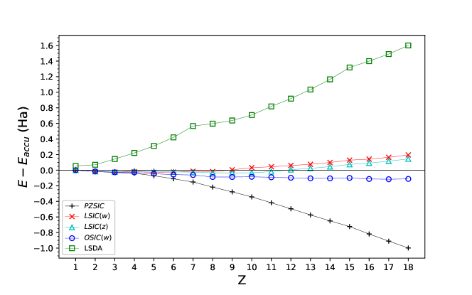
We compared the total atomic energies of the atoms against accurate non-relativistic values reported by Chakravorty et al.Chakravorty et al. (1993). Various integer values of were used for LSIC() and OSIC(). The differences between our calculated total energies with and the reference values are plotted in Fig. 1. The plot clearly shows the effect of scaling on the total energies of atoms. Consistent with reported results, the LSDA total energies are too high compared to accurate reference valuesChakravorty et al. (1993) whereas PZSIC consistently underestimates the total energies due to its over correcting tendency. The LSIC method, where both scaling factors performs similarly, provides the total energies closer to the reference values than LSDA and PZSIC-LSDA. Likewise, OSIC method also reduces the overcorrection bringing the total energies to close agreement with the reference values. The mean absolute errors (MAEs) in total energy with respect to the reference for various values are shown in Table 1. The MAE of PZSIC is Ha whereas LSIC() and OSIC() show MAEs of and Ha, respectively, with . LSIC() shows a better performance than OSIC() and LSIC(). The LSIC() MAE is in the same order of magnitude as the earlier reported MAE of LSIC() of 0.041 HaZope et al. (2019). As the value of increases, the magnitude of SI-correction is reduced. This result in MAEs become larger for eventually approaching the LSDA numbers.
For the scaled methods correctly produce the PZSIC results. The scaling is optimal for which results in optimal magnitude of SI-correction for LSIC() and almost right magnitude for OSIC(). The magnitude of SIC energy of each orbitals when compared among different methods, it is found that the SIC correction in LSIC() is larger (i.e. less scaling down) for the core orbitals than in the LSIC(). This trend is reversed for the valence orbitals (cf. Table 2). It can be seem from Table 2 that total SIC energy in both methods is essentially similar in magnitude. However the way scaling factors behave affects the orbitalwise contribution to the total SIC energy. This changes the SIC potentials and results in two methods performing differently for cations and anions. For OSIC(), we find the smallest MAE for of Ha, a value slightly smaller than that for .
| Method | MAE |
|---|---|
| PZSIC | 0.381 |
| LSIC() | 0.041 |
| LSIC() | 0.061 |
| LSIC() | 0.196 |
| LSIC() | 0.277 |
| LSIC() | 0.332 |
| OSIC() | 0.074 |
| OSIC() | 0.070 |
| OSIC() | 0.135 |
| Orbital | PZSIC | LSIC() | LSIC() | OSIC() |
|---|---|---|---|---|
| 1s | -0.741 | -0.387 | -0.490 | -0.584 |
| 2sp3 | -0.126 | -0.070 | -0.050 | -0.062 |
| 3sp3 | -0.016 | -0.017 | -0.006 | -0.008 |
| Total SIC | -2.616 | -1.473 | -1.421 | -1.729 |
III.1.2 Ionization potential
The ionization potential (IP) is the energy required to remove an electron from the outermost orbital. Since electron removal energy is related to the asymptotic shape of the potential, one can expect SIC plays an important role in determining IPs. We calculated the IPs using the SCF method defined as
| (10) |
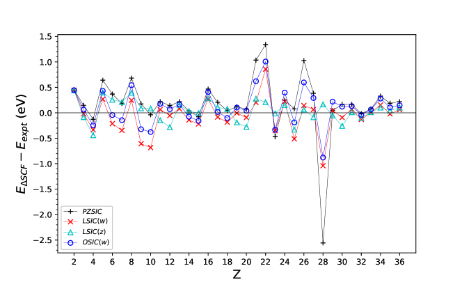
where is the total energy in the cationic state and is the total energy at the neutral state. The calculations were performed for atoms from helium to krypton, and we compared the computed IPs against the experimental ionization energies Kramida et al. (2018). FODs were relaxed both for neutral atoms and for their cations. Fig. 2 shows the difference of calculated IPs with respect to the reference values. MAEs with different methods are shown in Table 3 for a subset as well as for the entire set to facilitate a comparison against literature. For the smaller subset, , the MAEs are and eV for PZSIC and LSIC(), respectively. The MAE for OSIC(, ) is eV showing an improvement over PZSIC. LSIC(, ) shows MAE of eV, a comparable error with PZSIC. MAEs increase for LSIC(, ) and OSIC(, ) in comparison to their respective MAEs. Interestingly, however, when we considered the entire set of atoms (), LSIC() has MAEs of and eV for and respectively showing smaller errors than PZSIC (MAE, eV) but LSIC() falls short of LSIC() which has the smallest error (MAE, 0.170 eV). For this case, OSIC(, ) shows better performance than PZSIC but not as well as LSIC() for a given . LSIC() performs better than both LSIC() and OSIC(). The difference in performance between LSIC() and LSIC() implies that scaling of SIC for the cationic states is more sensitive to the choice of local scaling factor than for the neutral atoms.
| Method | Z=2-18 (17-IPs) | Z=2-36 (35-IPs) |
|---|---|---|
| PZSIC | 0.248 | 0.364 |
| LSIC() | 0.206 | 0.170 |
| LSIC() | 0.251 | 0.238 |
| LSIC() | 0.271 | 0.216 |
| LSIC() | 0.297 | 0.247 |
| LSIC() | 0.324 | 0.284 |
| OSIC() | 0.223 | 0.267 |
| OSIC() | 0.247 | 0.247 |
| OSIC() | 0.255 | 0.259 |
III.1.3 Electron affinity
The electron affinity (EA) is the energy released when an electron is added to the system. We studied EAs for 20 atoms that are experimentally found to bind an electronNational Institute of Standards and Technology . They are H, Li, B, C, O, F, Na, Al, Si, P, S, Cl, K, Ti, Cu, Ga, Ge, As, Se, and Br atoms. The EAs were calculated using the SCF method and values were compared against the experimental EAsNational Institute of Standards and Technology .
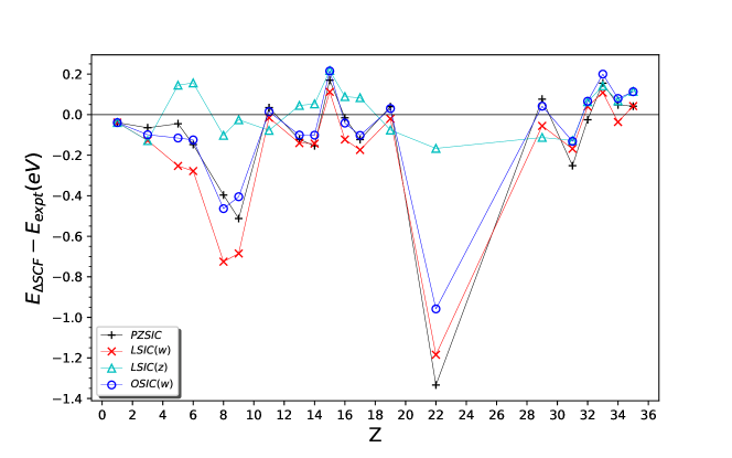
Fig. 3 shows deviation of EA from reference experimental values for various methods. The MAEs are summarized in Table 4. We have presented the MAEs in two sets, the smaller subset which contains hydrogen through chlorine (12 EAs) and for the complete set, hydrogen to bromine (20 EAs).
For 12 EAs, MAEs for PZSIC and LSIC() are and eV, respectively. OSIC() shows MAE of eV for , the same performance as PZSIC. LSIC(), however, does not perform as well as PZSIC, giving the MAEs of eV for . In both case, the error decrease slightly for but there is no significant impact on their performance.
For 20 EAs, the similar trend persists. PZSIC and LSIC() have MAEs of and eV, respectively. The MAEs of LSIC() are in the range eV for and those of OSIC() are between eV for . Again, decrease in error is observed as the value in increases. In particular, larger discrepancy between LSIC(,) and experiment is seen for O, F, and Ti atoms. This is due to LSIC() raising the anion energies more than their neutral state energies.
| Method | (12 EAs) MAE | (20 EAs) MAE |
|---|---|---|
| PZSIC | 0.152 | 0.190 |
| LSIC() | 0.097 | 0.102 |
| LSIC() | 0.235 | 0.224 |
| LSIC() | 0.229 | 0.205 |
| LSIC() | 0.215 | 0.189 |
| LSIC() | 0.202 | 0.176 |
| OSIC() | 0.152 | 0.172 |
| OSIC() | 0.150 | 0.164 |
| OSIC() | 0.145 | 0.155 |
III.2 Atomization energy
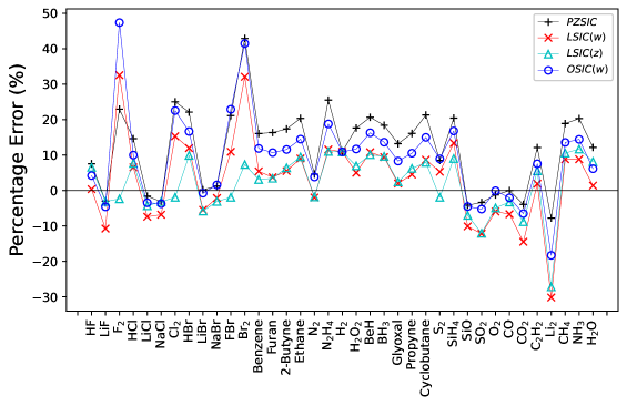
To study the performance of LSIC() for molecules, first, we calculated the atomization energies (AEs) of 37 selected molecules. Many of these molecules are subset of the G2/97 test setCurtiss et al. (1991). The 37 molecules set includes systems from the AE6 setLynch and Truhlar (2003), small but a good representative of the main group atomization energy (MGAE109) setPeverati and Truhlar (2011). The AEs were calculated by taking the energy difference of fragment atoms and the complex, that is, is the total energy of an atom, is the total energy of the molecule, and is the number of atoms in the molecule. The calculated AEs were compared to the non-spin-orbit coupling reference valuesPeverati and Truhlar (2011) for AE6 set and to the experimental valuesNational Institute of Standards and Technology for the entire set of 37 molecules. The percentage errors obtained through various methods are shown in Fig. 4. The overestimation of AEs with PZSIC-LSDA due to overcorrection is rectified in LSIC(). We have summarized MAEs and mean absolute percentage errors (MAPEs) of AE6 and 37 molecules from G2 set in Table 5. For AE6 set, MAEs for PZSIC, LSIC(), LSIC(), and OSIC() are , , , and kcal/mol respectively. The MAE in LSIC() is about 4 kcal/mol larger than LSIC() but substantially better than the PZSICs or OSIC(). For the larger in LSIC(), however, the performance starts to degrade with consistent increase in the MAE of kcal/mol for . This is in contrast to OSIC where the performance improves for and compared to . The scaling thus affect differently in the two methods. OSIC() tends to slightly underestimate total energies. By increasing , total energies shift toward the LSDA total energies and improves performance for moderate increase in . On the contrary, total energies are slightly overestimated for LSIC(), and increasing makes the energies deviate away from the accurate estimates. OSIC() and LSIC() have a similar core orbital SIC energy. In their study of OSIC(), Vydrov and ScuseriaVydrov and Scuseria (2006) used values of up to 5 and found the smallest error of (MAE, kcal/mol). But we expect the OSIC performance to degrade eventually for large since increase in results in increase in quenching of the SIC correction thus the results will eventually approach to those of DFA, in this case LSDA. For the full set of 37 molecules, PZSIC, LSIC(), LSIC(), and OSIC() show the MAPEs of , , and %, respectively. OSIC() shows a slight improvement in MAPE for and . For the larger set, LSIC() consistently shows smaller MAPEs than OSIC() for . All four values of with the LSIC() in this study showed better performance than PZSIC for the 37 molecules set.
| AE6 MAE | AE6 | 37 molecules | |
| Method | (kcal/mol) | MAPE (%) | MAPE (%) |
| PZSIC | 57.9 | 9.4 | 13.4 |
| LSIC( | 9.9 | 3.2 | 6.9 |
| LSIC() | 13.8 | 4.4 | 9.5 |
| LSIC() | 18.6 | 5.3 | 9.1 |
| LSIC() | 26.9 | 5.8 | 9.2 |
| LSIC() | 33.5 | 6.7 | 9.7 |
| OSIC() | 33.7 | 6.3 | 11.9 |
| OSIC() | 24.1 | 5.1 | 11.3 |
| OSIC() | 17.8 | 4.3 | 10.9 |
III.3 Barrier heights
Accurate description of chemical reaction barrier is challenging for DFAs since it involves calculation of energies in non-equilibrium situations. In most of the cases, the saddle point energies are underestimated since DFAs do not perform well for a non-equilibrium state that involves a stretched bond. This shortcoming of DFAs in a stretched bond case arises from SIE; when an electron is shared and stretched out, SIE incorrectly lowers the energy of transition state. SIC handles the stretched bond states accurately and provides a correct picture in chemical reaction paths. We studied the reaction barriers using the BH6Lynch and Truhlar (2003) set of molecules for LSIC() method. BH6 is a representative subset of the larger BH24Zheng et al. (2007) set consisting of three reactions OH + CH4 CH3 + H2O, H + OH H2 + O, and H + H2S H2 + HS. We calculated the total energies of left- and right-hand side and at the saddle point of these chemical reactions. The barrier heights for the forward (f) and reverse (r) reactions were obtained by taking the energy differences of their corresponding reaction states.
The mean errors (MEs) and MAEs of computed barrier heights against the reference valuesLynch and Truhlar (2003) are compared in Table 6. MAEs for PZSIC, LSIC(), LSIC(), and OSIC() are , , , and kcal/mol, respectively. PZSIC significantly improves MAE compared to LSDA (MAE, 17.6 kcal/mol), LSIC() further reduces the error from PZSIC. Its ME and MAE indicate that there is no systematic underestimation or overestimation. LSIC() also further improves the PZSIC numbers but not to the same level as LSIC(). For , MAEs increases systematically for LSIC() though small MEs are seen for LSIC(). The performance deteriorates for beyond that of PZSIC. OSIC() shows marginally better performance than PZSIC. Vydrov and ScuseriaVydrov and Scuseria (2006) showed that the best performance is achieved with (MAE, kcal/mol). The performance improvement with OSIC is not as dramatic as LSICs in terms of MEs and MAEs where the rather large MEs are seen i Overall LSIC() performs better than OSIC() for barrier heights.
| Method | ME (kcal/mol) | MAE (kcal/mol) |
|---|---|---|
| PZSIC | -4.8 | 4.8 |
| LSIC() | 0.7 | 1.3 |
| LSIC() | -1.0 | 3.6 |
| LSIC() | -0.1 | 4.6 |
| LSIC() | 0.3 | 5.0 |
| LSIC() | 0.6 | 5.5 |
| OSIC() | -3.4 | 3.6 |
| OSIC() | -3.1 | 4.1 |
| OSIC() | -3.0 | 4.6 |
III.4 Dissociation and reaction energies
A pronounced manifestation of SIE is seen in dissociation of positively charged dimers . SIE causes the system to dissociate into two fractionally charges cations instead of and . Here we use the SIE4x4Goerigk et al. (2017) and SIE11Goerigk and Grimme (2010) sets to study the performance of LSIC() and OSIC() in correcting the SIEs. The SIE4x4 set consists of dissociation energy calculations of four positively charged dimers at varying bond distances from their equilibrium distance such that = 1.0, 1.25, 1.5 and 1.75. The dissociation energy is calculated as
| (11) |
The SIE11 set consists of eleven reaction energy calculations: five cationic reactions and six neutral reactions. These two sets are commonly used for studying the SIE related problems. The calculated dissociation and reaction energies are compared against the CCSD(T) reference valuesGoerigk et al. (2017); Goerigk and Grimme (2010), and MAEs are summarized in Table 7. For the SIE4x4 set, PZSIC, LSIC(), LSIC(), and OSIC() show MAEs of , , and kcal/mol. LSIC() provides small improvement in equilibrium energies while keeping accurate behavior of PZSIC at the dissociation limit resulting in marginally better performance. LSIC() shows errors a few kcal/mol larger than PZSIC. This increase in error arises because LSIC() alters the (NH3) and (H2O) dissociation curves. In LSIC() the scaling of SIC occurs mostly for the core orbitals (Cf. Table 2) whereas LSIC() also includes some noticeable scaling down effect from valence orbitals. This different scaling behavior seems to contribute to different dissociation curves. Lastly, OSIC() has a slightly larger error than LSIC().
For the SIE11 set, MAEs are , , , and kcal/mol for PZSIC, LSIC(), LSIC(), and OSIC(), respectively. All scaled-down approaches we considered, LSIC() and LSIC(), and OSIC() showed performance improvement over PZSIC. LSIC() shows the largest error reduction by 60%, while LSIC() shows 28% decrease in error with respect to PZSIC. OSIC() with has slightly smaller MAEs within 1 kcal/mol of PZSIC. LSIC() method improves cationic reactions more than neutral reactions with respect to PZSIC. Increase in beyond 2 results in too much suppression of SIC and leads to increase in error for LSIC(). LSIC() yielded consistently smaller MAEs than OSIC() but larger than LSIC() over the whole SIE11 reactions.
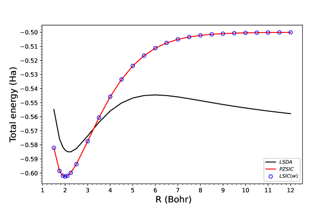
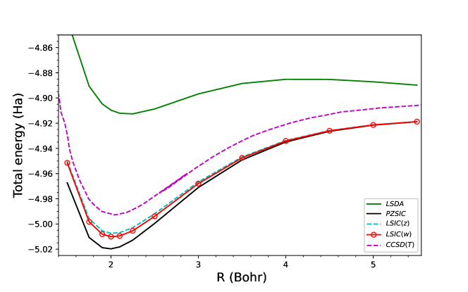
Finally, we show the ground-state dissociation curves for H and He in Fig. 5. As previously discussed in literature Ruzsinszky et al. (2005), DFAs at large separation cause the complexes to dissociate into two fragments atoms. PZSIC restores the correct dissociation behavior at the large separation distance. When LSIC is applied, the behavior of PZSIC at the dissociation limit is preserved in both LSIC() and present LSIC(). For H, a one-electron system, LSIC reproduces the identical behavior as PZSIC [Fig. 5 (a)]. For He, a three-electron system, LSIC applies the correction to PZSIC only near equilibrium regime [Fig. 5 (b)]. LSIC brings the equilibrium energy closer to the CCSD energy compared to PZSIC energy. The implication of Fig. 5 is that the present scaling factor performs well in differentiating the single-orbital like regions and many-electron like regions.
| Reaction | SIE4x4 | SIE11 | SIE11 | SIE11 |
|---|---|---|---|---|
| 5 cationic | 6 neutral | |||
| PZSIC | 3.0 | 11.5 | 14.9 | 8.7 |
| LSIC() | 2.6 | 4.5 | 2.3 | 6.3 |
| LSIC() (k=1) | 4.7 | 8.3 | 8.6 | 8.0 |
| LSIC() (k=2) | 5.5 | 8.3 | 8.3 | 8.3 |
| LSIC() (k=3) | 5.8 | 8.8 | 8.2 | 9.3 |
| LSIC() (k=4) | 5.9 | 9.3 | 8.2 | 10.2 |
| OSIC() (k=1) | 5.2 | 11.1 | 13.7 | 9.0 |
| OSIC() (k=2) | 6.0 | 11.0 | 13.5 | 9.0 |
| OSIC() (k=3) | 6.4 | 10.9 | 13.3 | 8.8 |
III.5 Water binding energies: a case where LSIC() performs poorly
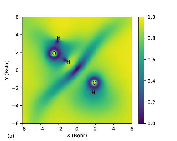
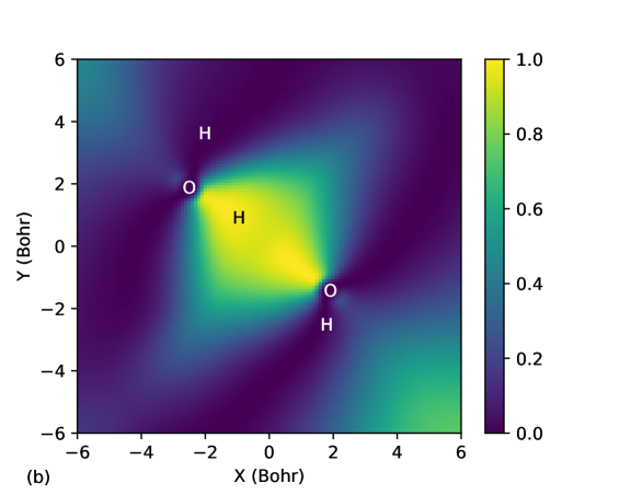
Kamal et al.Sharkas et al. (2020) recently studied binding energies of small water clusters using the PZSIC method in conjunction with FLOs to examine the effect of SIC on binding energies of these systems. Water clusters are bonded by weaker hydrogen bonds and provide a different class of systems to test the performance of the LSIC method. Earlier studies using LSIC() on the polarizabilities and ionization have shown that LSIC() provides an excellent descriptions of these properties when compared to the CCSD(T) resultsVargas et al. (2020); Akter et al. . Here, we study the binding energies of the water clusters. We find that the choice of iso-orbital indicator plays crucial role in water cluster binding energies. The structures considered in this work are (H2O)n () whose geometries are from the WATER27 setBryantsev et al. (2009) optimized at the B3LYP/6-311++G(2d,2p) theory. The hexamer structure has a few known isomers, and we considered the book (b), cage (c), prism (p), and ring (r) isomers. The results are compared against the CCSD(T)-F12b values from Ref. [Manna et al., 2017] in Table 8. We obtained the MAEs of 118.9, 172.1, and 46.9 meV/H2O for PZSIC, LSIC(), and LSIC(), respectively. Thus, LSIC() underestimates binding energies of water cluster by roughly similar magnitude as LSDA (MAE, 183.4 meV/H2O). This is one case where LSIC() does not improve over PZSIC. A simple explanation for this behavior of LSIC() is that although used in LSIC() can detect the weak bond regions, it () cannot differentiate the slow-varying density regions from weak bond regions. The in the both situations causing the weak regions to be improperly treated. Fig. 6 (a) shows for water dimer where both slow-varying density and weak interaction regions are detected but not differentiated. As a result, the total energies of the complex shift too much in comparison to the individual water molecules. Thus, the underestimation of water cluster binding energies is due to the choice of and not the LSIC method. Indeed by choosing the as a scaling parameter, the binding energies are much improved. Fig. 6 (b) shows there is no discontinuity of between the two water molecules (’s of two FLOs along the hydrogen bond are plotted together in the figure). Hence unlike in LSIC(), weak interacting region is not improperly scaled down with LSIC(). LSIC() shows MAE of 46.9 meV/H2O comparable to SCAN (MAE, 35.2 meV/H2O). This result is interesting as SCAN uses a function that can identify weak bond interaction. So LSIC()-LSDA may be behaving qualitatively similar to the detection function in SCAN in weak bond regions. The study of water binding energies is so far a unique case where the original LSIC() performed poorly. But LSIC can be improved by simply using a different iso-orbital indicator. This case serves as a motivation in identifying appropriate iso-orbital indicator that would work for all bonding regions in LSIC.
| PZSIC | LSIC() | LSIC() | CCSD(T) | |
| 2 | -153.7 | -34.9 | -82.7 | -108.6 |
| 3 | -321.6 | -73.9 | -183.0 | -228.4 |
| 4 | -425.2 | -125.0 | -248.6 | -297.0 |
| 5 | -446.9 | -142.7 | -264.8 | -311.4 |
| 6b | -467.1 | -133.6 | -275.0 | -327.3 |
| 6c | -466.8 | -113.9 | -274.8 | -330.5 |
| 6p | -467.7 | -104.8 | -276.2 | -332.4 |
| 6r | -458.1 | -150.5 | -275.5 | -320.1 |
| MAE | 118.9 | 172.1 | 46.9 | |
| Reference [Manna et al., 2017] | ||||
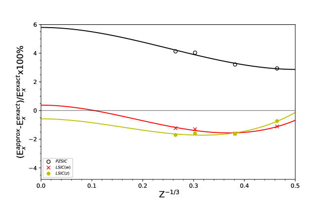
We now provide a qualitative explanation of why LSIC() gives improved results over PZSIC. This reasoning is along the same line as offered by Zope et al. Zope et al. (2019). As mentioned in Sec. I, when the self-interaction-errors are removed using PZSIC, improved description of barrier heights which involve stretch bonds is obtained but the equilibrium properties like total energies, atomization energies etc. are usually deteriorated compared to the uncorrected functional. This is especially so for the functionals that go beyond the simple LSDA. Typically this is because of over correcting tendency of PZSIC. The non-empirical semilocal DFA functionals are designed to be exact in the uniform electron gas limit, this exact condition is no longer satisfied when PZSIC is applied to the functionalsSantra and Perdew (2019). This can be seen from the exchange energies of noble gas atoms and the extrapolation using the large- expansion of as shown in Fig. 7. Following Ref. [Santra and Perdew, 2019] we plot atomic exchange energies as a function of . Thus, the region near origin corresponds to the uniform gas limit. The plot was obtained by fitting the exchange exchange energies () of Ne, Ar, Kr, and Xe atoms (within LSIC()-LSDA, LSIC()-LSDA, and LSDA) for Ne, Ar, Kr, and Xe atoms to the curve using the following fitting functionSantra and Perdew (2019).
| (12) |
where and a, b, and c are the fitting parameters. The LSDA is exact in the uniform gas limit. So also is LSIC() since the scaling factor approaches zero as the gradient of electron density vanishes while the kinetic energy density in the denominator remains finite. The small deviation from zero seen near origin (in Fig. 7) for LSIC() is due to the fitting error (due to limited data point). This error is for LSIC(). Thus correcting LSDA using PZSIC introduces large error in the uniform gas limit. The scaling factor used here identifies single-electron region since the density ratio approaches one in this limit. Fig. 7 shows that present LSIC() approach also recovers the lost uniform limit gas. This partly explains the success of LSIC(). Though performance of LSIC () is substantially better than PZSIC-LSDA it falls short of LSIC(). On the other hand, unlike LSIC() it provides good description of weak hydrogen bonds highlighting the need of identifying suitable iso-orbital indicators or scaling factor(s) to apply pointwise SIC using LSIC method. One possible choice may be scaling factor that are functions of used in construction of SCAN meta-GGA and recently proposedFurness and Sun (2019) parameter. A scaling factor containing recently used by Yamamoto and coworkers with OSIC scheme showed improved resultsYamamoto et al. (2020). Future work would involve designing suitable scaling factors involving for use in LSIC method.
IV Conclusions
To recapitulate, we investigated the performance of LSIC with a simple scaling factor, , that depends only on orbital and spin densities. Performance assessment has been carried out on atomic energies, atomization energies, ionization potentials, electron affinities, barrier heights, dissociation energies etc on standard data sets of molecules. The results show that LSIC() performs better than PZSIC for all properties with exception of electron affinity and a SIE4x4 subset of dissociation energies. We also compared the performance of for LSIC against OSIC of Vydrov et al. Results indicate that although OSIC overall performs better than PZSIC, the improvement over PZSIC is somewhat limited. On the other hand, LSIC() is consistently better than OSIC(). We have also studied the binding energies of small water clusters which are bonded by weak hydrogen bonds. Here, the LSIC() performs very well compared to both the PZSIC and LSIC() with performance comparable to SCAN. The present work shows the promise of LSIC method and also demonstrates its limitation in describing weak hydrogen bonds if used with kinetic energy ratio, as an iso-orbital indicator. This limitation is due to inability of to distinguish weak bonding regions from slowly varying density regions. The scaling factor works differently than the scaling factor , hence LSIC() provides good description of weak hydrogen bonds in water clusters. The work thus highlights importance of designing suitable iso-orbital indicator for use with LSIC that can detect weak bonding regions.
Data Availability Statement
The data that supports the findings of this study are available within the article and the supplementary information.
Conflicts of interest
There are no conflicts of interest to declare.
Acknowledgement
Authors acknowledge Drs. Luis Basurto, Carlos Diaz, and Po-Hao Chang for discussions and technical supports. This work was supported by the US Department of Energy, Office of Science, Office of Basic Energy Sciences, as part of the Computational Chemical Sciences Program under Award No. DE-SC0018331. Support for computational time at the Texas Advanced Computing Center through NSF Grant No. TG-DMR090071, and at NERSC is gratefully acknowledged.
References
- Kohn and Sham (1965) W. Kohn and L. Sham, Phys. Rev., 1965, 140, A1133–A1138.
- Jones (2015) R. O. Jones, Rev. Mod. Phys., 2015, 87, 897.
- Jones and Gunnarsson (1989) R. O. Jones and O. Gunnarsson, Rev. Mod. Phys., 1989, 61, 689–746.
- Perdew and Zunger (1981) J. P. Perdew and A. Zunger, Phys. Rev. B, 1981, 23, 5048–5079.
- Perdew and Schmidt (2001) J. P. Perdew and K. Schmidt, AIP Conference Proceedings, 2001, 577, 1–20.
- Johnson et al. (2008) E. R. Johnson, P. Mori-Sánchez, A. J. Cohen and W. Yang, The Journal of Chemical Physics, 2008, 129, 204112.
- Johnson et al. (2013) E. R. Johnson, A. Otero-de-la Roza and S. G. Dale, The Journal of Chemical Physics, 2013, 139, 184116.
- Gräfenstein et al. (2004) J. Gräfenstein, E. Kraka and D. Cremer, J. Chem. Phys., 2004, 120, 524–539.
- Lindgren (1971) I. Lindgren, Int. J. Quantum Chem., 1971, 5, 411–420.
- Gopinathan (1977) M. S. Gopinathan, Phys. Rev. A, 1977, 15, 2135–2142.
- Perdew et al. (1982) J. P. Perdew, R. G. Parr, M. Levy and J. L. Balduz Jr, Physical Review Letters, 1982, 49, 1691.
- Lundin and Eriksson (2001) U. Lundin and O. Eriksson, Int. J. Quantum Chem., 2001, 81, 247–252.
- Mori-Sánchez et al. (2006) P. Mori-Sánchez, A. J. Cohen and W. Yang, The Journal of Chemical Physics, 2006, 125, 201102.
- Gidopoulos and Lathiotakis (2012) N. I. Gidopoulos and N. N. Lathiotakis, The Journal of Chemical Physics, 2012, 136, 224109.
- Tsuneda et al. (2003) T. Tsuneda, M. Kamiya and K. Hirao, J. Comput. Chem., 2003, 24, 1592–1598.
- Vydrov and Scuseria (2006) O. A. Vydrov and G. E. Scuseria, J. Chem. Phys., 2006, 124, 191101.
- Zope et al. (2019) R. R. Zope, Y. Yamamoto, C. M. Diaz, T. Baruah, J. E. Peralta, K. A. Jackson, B. Santra and J. P. Perdew, J. Chem. Phys., 2019, 151, 214108.
- Seo (2007) D.-K. Seo, Phys. Rev. B, 2007, 76, 033102.
- Tsuneda and Hirao (2014) T. Tsuneda and K. Hirao, The Journal of Chemical Physics, 2014, 140, 18A513.
- Slater (1951) J. C. Slater, Physical review, 1951, 81, 385.
- Ruzsinszky et al. (2007) A. Ruzsinszky, J. P. Perdew, G. I. Csonka, O. A. Vydrov and G. E. Scuseria, J. Chem. Phys., 2007, 126, 104102.
- Garza et al. (2000) J. Garza, J. A. Nichols and D. A. Dixon, J. Chem. Phys., 2000, 112, 7880–7890.
- Garza et al. (2001) J. Garza, R. Vargas, J. A. Nichols and D. A. Dixon, J. Chem. Phys., 2001, 114, 639–651.
- Patchkovskii et al. (2001) S. Patchkovskii, J. Autschbach and T. Ziegler, J. Chem. Phys., 2001, 115, 26–42.
- Harbola (1996) M. K. Harbola, Solid State Commun., 1996, 98, 629–632.
- Patchkovskii and Ziegler (2002) S. Patchkovskii and T. Ziegler, J. Chem. Phys., 2002, 116, 7806–7813.
- Patchkovskii and Ziegler (2002) S. Patchkovskii and T. Ziegler, J. Phys. Chem. A, 2002, 106, 1088–1099.
- Goedecker and Umrigar (1997) S. Goedecker and C. J. Umrigar, Phys. Rev. A, 1997, 55, 1765–1771.
- Polo et al. (2002) V. Polo, E. Kraka and D. Cremer, Molecular Physics, 2002, 100, 1771–1790.
- Polo et al. (2003) V. Polo, J. Gräfenstein, E. Kraka and D. Cremer, Theor. Chem. Acc., 2003, 109, 22–35.
- Gräfenstein et al. (2004) J. Gräfenstein, E. Kraka and D. Cremer, Phys. Chem. Chem. Phys., 2004, 6, 1096–1112.
- Vydrov and Scuseria (2004) O. A. Vydrov and G. E. Scuseria, J. Chem. Phys., 2004, 121, 8187–8193.
- Vydrov and Scuseria (2005) O. A. Vydrov and G. E. Scuseria, J. Chem. Phys., 2005, 122, 184107.
- Vydrov et al. (2006) O. A. Vydrov, G. E. Scuseria, J. P. Perdew, A. Ruzsinszky and G. I. Csonka, J. Chem. Phys., 2006, 124, 094108.
- Zope et al. (1999) R. R. Zope, M. K. Harbola and R. K. Pathak, The European Physical Journal D-Atomic, Molecular, Optical and Plasma Physics, 1999, 7, 151–155.
- Zope (2000) R. R. Zope, Physical Review A, 2000, 62, 064501.
- Fois et al. (1993) E. S. Fois, J. I. Penman and P. A. Madden, The Journal of chemical physics, 1993, 98, 6352–6360.
- Krieger et al. (1992) J. B. Krieger, Y. Li and G. J. Iafrate, Phys. Rev. A, 1992, 45, 101–126.
- Krieger et al. (1992) J. B. Krieger, Y. Li and G. J. Iafrate, Phys. Rev. A, 1992, 46, 5453–5458.
- Li et al. (1993) Y. Li, J. B. Krieger and G. J. Iafrate, Phys. Rev. A, 1993, 47, 165–181.
- Lehtola et al. (2016) S. Lehtola, M. Head-Gordon and H. Jónsson, J. Chem. Theory Comput., 2016, 12, 3195–3207.
- Csonka and Johnson (1998) G. I. Csonka and B. G. Johnson, Theor. Chim. Acta, 1998, 99, 158–165.
- Petit et al. (2014) L. Petit, A. Svane, M. Lüders, Z. Szotek, G. Vaitheeswaran, V. Kanchana and W. Temmerman, J. Phys. Cond. Matter, 2014, 26, 274213.
- Kümmel and Kronik (2008) S. Kümmel and L. Kronik, Rev. Mod. Phys., 2008, 80, 3.
- Schmidt et al. (2014) T. Schmidt, E. Kraisler, L. Kronik and S. Kümmel, Phys. Chem. Chem. Phys., 2014, 16, 14357–14367.
- Kao et al. (2017) D.-y. Kao, M. Pederson, T. Hahn, T. Baruah, S. Liebing and J. Kortus, Magnetochemistry, 2017, 3, 31.
- Schwalbe et al. (2018) S. Schwalbe, T. Hahn, S. Liebing, K. Trepte and J. Kortus, J. Comput. Chem., 2018, 39, 2463–2471.
- Jónsson et al. (2007) H. Jónsson, K. Tsemekhman and E. J. Bylaska, Abstracts of Papers of the American Chemical Society, 2007, pp. 120–120.
- Rieger and Vogl (1995) M. M. Rieger and P. Vogl, Phys. Rev. B, 1995, 52, 16567.
- Temmerman et al. (1999) W. Temmerman, A. Svane, Z. Szotek, H. Winter and S. Beiden, Electronic Structure and Physical Properies of Solids, Springer, 1999, pp. 286–312.
- Daene et al. (2009) M. Daene, M. Lueders, A. Ernst, D. Ködderitzsch, W. M. Temmerman, Z. Szotek and W. Hergert, J. Phys. Cond. Matter, 2009, 21, 045604.
- Szotek et al. (1991) Z. Szotek, W. Temmerman and H. Winter, Physica B: Condensed Matter, 1991, 172, 19–25.
- Messud et al. (2008) J. Messud, P. M. Dinh, P.-G. Reinhard and E. Suraud, Phys. Rev. Lett., 2008, 101, 096404.
- Messud et al. (2008) J. Messud, P. M. Dinh, P.-G. Reinhard and E. Suraud, Chem. Phys. Lett., 2008, 461, 316–320.
- Lundberg and Siegbahn (2005) M. Lundberg and P. E. M. Siegbahn, J. Chem. Phys., 2005, 122, 224103.
- Körzdörfer et al. (2008) T. Körzdörfer, M. Mundt and S. Kümmel, Phys. Rev. Lett., 2008, 100, 133004.
- Körzdörfer et al. (2008) T. Körzdörfer, S. Kümmel and M. Mundt, J. Chem. Phys., 2008, 129, 014110.
- Ciofini et al. (2005) I. Ciofini, C. Adamo and H. Chermette, Chem. Phys., 2005, 309, 67–76.
- Baruah et al. (1994) T. Baruah, R. R. Zope, A. Kshirsagar and R. K. Pathak, Phys. Rev. A, 1994, 50, 2191–2196.
- Johnson et al. (2019) A. I. Johnson, K. P. K. Withanage, K. Sharkas, Y. Yamamoto, T. Baruah, R. R. Zope, J. E. Peralta and K. A. Jackson, J. Chem. Phys., 2019, 151, 174106.
- Vargas et al. (2020) J. Vargas, P. Ufondu, T. Baruah, Y. Yamamoto, K. A. Jackson and R. R. Zope, Phys. Chem. Chem. Phys., 2020, 22, 3789–3799.
- Trepte et al. (2019) K. Trepte, S. Schwalbe, T. Hahn, J. Kortus, D.-Y. Kao, Y. Yamamoto, T. Baruah, R. R. Zope, K. P. K. Withanage, J. E. Peralta and K. A. Jackson, J. Comput. Chem., 2019, 40, 820–825.
- Withanage et al. (2018) K. P. K. Withanage, K. Trepte, J. E. Peralta, T. Baruah, R. Zope and K. A. Jackson, J. Chem. Theory Comput., 2018, 14, 4122–4128.
- Pederson et al. (2016) M. R. Pederson, T. Baruah, D.-y. Kao and L. Basurto, J. Chem. Phys., 2016, 144, 164117.
- Schwalbe et al. (2019) S. Schwalbe, L. Fiedler, T. Hahn, K. Trepte, J. Kraus and J. Kortus, PyFLOSIC - Python based Fermi-Löwdin orbital self-interaction correction, 2019.
- Kao et al. (2017) D.-y. Kao, K. Withanage, T. Hahn, J. Batool, J. Kortus and K. Jackson, J. Chem. Phys., 2017, 147, 164107.
- Joshi et al. (2018) R. P. Joshi, K. Trepte, K. P. K. Withanage, K. Sharkas, Y. Yamamoto, L. Basurto, R. R. Zope, T. Baruah, K. A. Jackson and J. E. Peralta, J. Chem. Phys., 2018, 149, 164101.
- Sharkas et al. (2018) K. Sharkas, L. Li, K. Trepte, K. P. K. Withanage, R. P. Joshi, R. R. Zope, T. Baruah, J. K. Johnson, K. A. Jackson and J. E. Peralta, J. Phys. Chem. A, 2018, 122, 9307–9315.
- Jackson et al. (2019) K. A. Jackson, J. E. Peralta, R. P. Joshi, K. P. Withanage, K. Trepte, K. Sharkas and A. I. Johnson, J. Phys. Conf. Ser., 2019, 1290, 012002.
- Sharkas et al. (2020) K. Sharkas, K. Wagle, B. Santra, S. Akter, R. R. Zope, T. Baruah, K. A. Jackson, J. P. Perdew and J. E. Peralta, Proceedings of the National Academy of Sciences, 2020, 117, 11283–11288.
- Pederson et al. (1984) M. R. Pederson, R. A. Heaton and C. C. Lin, J. Chem. Phys., 1984, 80, 1972–1975.
- Pederson et al. (1985) M. R. Pederson, R. A. Heaton and C. C. Lin, J. Chem. Phys., 1985, 82, 2688–2699.
- Luken and Beratan (1982) W. L. Luken and D. N. Beratan, Theor. Chem. Acc., 1982, 61, 265–281.
- Luken and Culberson (1984) W. L. Luken and J. C. Culberson, Theor. Chem. Acc., 1984, 66, 279–293.
- Pederson et al. (2014) M. R. Pederson, A. Ruzsinszky and J. P. Perdew, J. Chem. Phys., 2014, 140, 121103.
- Pederson and Baruah (2015) M. R. Pederson and T. Baruah, Advances In Atomic, Molecular, and Optical Physics, Academic Press, 2015, vol. 64, pp. 153–180.
- Joshi et al. (2016) R. P. Joshi, J. J. Phillips and J. E. Peralta, Journal of Chemical Theory and Computation, 2016, 12, 1728–1734.
- (78) R. R. Zope, T. Baruah and K. A. Jackson, FLOSIC 0.2, https://http://flosic.org/, based on the NRLMOL code of M. R. Pederson.
- Withanage et al. (2019) K. P. K. Withanage, S. Akter, C. Shahi, R. P. Joshi, C. Diaz, Y. Yamamoto, R. Zope, T. Baruah, J. P. Perdew, J. E. Peralta and K. A. Jackson, Phys. Rev. A, 2019, 100, 012505.
- Shahi et al. (2019) C. Shahi, P. Bhattarai, K. Wagle, B. Santra, S. Schwalbe, T. Hahn, J. Kortus, K. A. Jackson, J. E. Peralta, K. Trepte, S. Lehtola, N. K. Nepal, H. Myneni, B. Neupane, S. Adhikari, A. Ruzsinszky, Y. Yamamoto, T. Baruah, R. R. Zope and J. P. Perdew, J. Chem. Phys., 2019, 150, 174102.
- Yamamoto et al. (2019) Y. Yamamoto, C. M. Diaz, L. Basurto, K. A. Jackson, T. Baruah and R. R. Zope, J. Chem. Phys., 2019, 151, 154105.
- (82) M. R. Pederson and T. Baruah, unpublished.
- Yamamoto et al. (2020) Y. Yamamoto, S. Romero, T. Baruah and R. R. Zope, The Journal of Chemical Physics, 2020, 152, 174112.
- Klüpfel et al. (2012) S. Klüpfel, P. Klüpfel and H. Jónsson, J. Chem. Phys., 2012, 137, 124102.
- Klüpfel et al. (2011) S. Klüpfel, P. Klüpfel and H. Jónsson, Phys. Rev. A, 2011, 84, 050501.
- Jónsson et al. (2015) E. Ö. Jónsson, S. Lehtola and H. Jónsson, Procedia Computer Science, 2015, 51, 1858–1864.
- Perdew et al. (2015) J. P. Perdew, A. Ruzsinszky, J. Sun and M. R. Pederson, Advances In Atomic, Molecular, and Optical Physics, Academic Press, 2015, vol. 64, pp. 1–14.
- Ruzsinszky et al. (2006) A. Ruzsinszky, J. P. Perdew, G. I. Csonka, O. A. Vydrov and G. E. Scuseria, J. Chem. Phys., 2006, 125, 194112.
- Jaramillo et al. (2003) J. Jaramillo, G. E. Scuseria and M. Ernzerhof, J. Chem. Phys., 2003, 118, 1068–1073.
- Schmidt et al. (2014) T. Schmidt, E. Kraisler, A. Makmal, L. Kronik and S. K ummel, The Journal of Chemical Physics, 2014, 140, 18A510.
- Slater and Wood (1970) J. C. Slater and J. H. Wood, International Journal of Quantum Chemistry, 1970, 5, 3–34.
- Heaton et al. (1983) R. A. Heaton, J. G. Harrison and C. C. Lin, Phys. Rev. B, 1983, 28, 5992–6007.
- Harrison et al. (1983) J. G. Harrison, R. A. Heaton and C. C. Lin, Journal of Physics B: Atomic and Molecular Physics, 1983, 16, 2079–2091.
- (94) Y. Yamamoto, L. Basurto, C. M. Diaz, R. R. Zope and T. Baruah, Self-interaction correction to density functional approximations using Fermi-Löwdin orbitals: methodology and parallelization, Unpublished.
- Porezag and Pederson (1999) D. Porezag and M. R. Pederson, Phys. Rev. A, 1999, 60, 2840–2847.
- Pederson and Jackson (1990) M. R. Pederson and K. A. Jackson, Phys. Rev. B, 1990, 41, 7453–7461.
- Bhattarai et al. (2020) P. Bhattarai, K. Wagle, C. Shahi, Y. Yamamoto, S. Romero, B. Santra, R. R. Zope, J. E. Peralta, K. A. Jackson and J. P. Perdew, The Journal of Chemical Physics, 2020, 152, 214109.
- Chakravorty et al. (1993) S. J. Chakravorty, S. R. Gwaltney, E. R. Davidson, F. A. Parpia and C. F. p Fischer, Phys. Rev. A, 1993, 47, 3649–3670.
- Kramida et al. (2018) A. Kramida, Yu. Ralchenko, J. Reader and NIST ASD Team, NIST Atomic Spectra Database (ver. 5.6.1), [Online]. Available: https://physics.nist.gov/asd [2018, July 25]. National Institute of Standards and Technology, Gaithersburg, MD., 2018.
- (100) National Institute of Standards and Technology, NIST Computational Chemistry Comparison and Benchmark Database NIST Standard Reference Database Number 101 Release 19, April 2018, Editor: Russell D. Johnson III http://cccbdb.nist.gov/ DOI:10.18434/T47C7Z.
- Curtiss et al. (1991) L. A. Curtiss, K. Raghavachari, G. W. Trucks and J. A. Pople, J. Chem. Phys., 1991, 94, 7221–7230.
- Lynch and Truhlar (2003) B. J. Lynch and D. G. Truhlar, J. Phys. Chem. A, 2003, 107, 8996–8999.
- Peverati and Truhlar (2011) R. Peverati and D. G. Truhlar, J. Chem. Phys., 2011, 135, 191102.
- Zheng et al. (2007) J. Zheng, Y. Zhao and D. G. Truhlar, J. Chem. Theory Comput., 2007, 3, 569–582.
- Goerigk et al. (2017) L. Goerigk, A. Hansen, C. Bauer, S. Ehrlich, A. Najibi and S. Grimme, Phys. Chem. Chem. Phys., 2017, 19, 32184–32215.
- Goerigk and Grimme (2010) L. Goerigk and S. Grimme, J. Chem. Theory Comput., 2010, 6, 107–126.
- Ruzsinszky et al. (2005) A. Ruzsinszky, J. P. Perdew and G. I. Csonka, The Journal of Physical Chemistry A, 2005, 109, 11006–11014.
- (108) S. Akter, Y. Yamamoto, C. M. Diaz, K. A. Jackson, R. R. Zope and T. Baruah.
- Bryantsev et al. (2009) V. S. Bryantsev, M. S. Diallo, A. C. T. van Duin and W. A. Goddard, Journal of Chemical Theory and Computation, 2009, 5, 1016–1026.
- Manna et al. (2017) D. Manna, M. K. Kesharwani, N. Sylvetsky and J. M. L. Martin, J. Chem. Theory Comput., 2017, 13, 3136–3152.
- Santra and Perdew (2019) B. Santra and J. P. Perdew, J. Chem. Phys., 2019, 150, 174106.
- Furness and Sun (2019) J. W. Furness and J. Sun, Phys. Rev. B, 2019, 99, 041119.