Local Structure-aware Graph Contrastive Representation Learning
Abstract
Traditional Graph Neural Network (GNN), as a graph representation learning method, is constrained by label information. However, Graph Contrastive Learning (GCL) methods, which tackle the label problem effectively, mainly focus on the feature information of the global graph or small subgraph structure (e.g., the first-order neighborhood). In the paper, we propose a Local Structure-aware Graph Contrastive representation Learning method (LSGCL) to model the structural information of nodes from multiple views. Specifically, we construct the semantic subgraphs that are not limited to the first-order neighbors. For the local view, the semantic subgraph of each target node is input into a shared GNN encoder to obtain the target node embeddings at the subgraph-level. Then, we use a pooling function to generate the subgraph-level graph embeddings. For the global view, considering the original graph preserves indispensable semantic information of nodes, we leverage the shared GNN encoder to learn the target node embeddings at the global graph-level. The proposed LS-GCL model is optimized to maximize the common information among similar instances at three various perspectives through a multi-level contrastive loss function. Experimental results on five datasets illustrate that our method outperforms state-of-the-art graph representation learning approaches for both node classification and link prediction tasks.
keywords:
Graph representation learning , Graph neural network , Self-supervised learning , Graph contrastive learning[inst1]organization=College of Information Engineering, Yangzhou University,city=Yangzhou, postcode=225127, country=China
[inst2]organization=Business School, University of Shanghai for Science and Technology,city=Shanghai, postcode=200093, country=China
1 Introduction
Graph neural network (GNN)[1, 2, 3] has made noteworthy progress in processing the graph-structured data. The core idea of GNN models, such as the graph convolutional network (GCN) [4] and graph attention network (GAT) [5], is to extract the structural information of nodes by transmitting and aggregating the attribute information of neighbors, and generate the embedding representations of nodes in the low-dimensional embedding space. The GNNs have widespread applications in real life, including the recommendation system [6], intelligent transportation system [7] and drug development in the biomedical field [8], etc. However, traditional GNN methods, belonging to (semi-)supervised learning [9, 10], are constrained by the label information, which is difficult to acquire in practical applications due to the privacy protection [11]. The uneven distribution of labels or the false labels also affect the realistic performance of the GNN models [12].
The unlabeled graph data (e.g., the adjacency matrix) is accessible compared with manual label information in real world. Graph contrastive learning (GCL) [13], as a popular self-supervised learning technique which utilizes known graph data to mine feature information of nodes or graphs, has attracted extensive researches. The core idea of GCL is to set the positive and negative sample objects according to the original graph information, and maximize the feature information between the target nodes and positive samples, minimize the common feature information between the target nodes and negative samples in the training process[14]. Nodes with similar properties in the graph will generate close embedding representations in the embedding space. Recent GCL works have achieved excellent results in various downstream tasks, such as node classification [15], graph classification [16] and link prediction [17]. According to the contrastive objectives, existing GCL models can be summarized into three categories. The first is the Node-Graph level contrastive learning framework, which maximizes the common information between the target node embeddings (local graph structure) and the graph embedding of the global graph (global graph structure), such as the DGI[18]. The second is the Node-Node level contrastive learning framework, which maximizes the consistency of feature information between the target node embeddings (local graph structure) and the positive sample node embeddings (local graph structure), such as the GRACE[19], GCA[20], GMI[21]. The third is the Node-Subgraph level contrastive learning framework, which maximizes the common information between the target node embeddings (local graph structure) and the subgraph-level graph embedding (local graph structure), such as MVGRL[22], SUBG-CON[23]. Among the three frameworks mentioned above, existing GCL models mainly focus on the global graph or small subgraph structure (e.g., the first-order neighborhood).
How to maximize the local feature information of nodes while preserving the global features of the original graph is a challenge. In the paper, we propose a novel graph contrastive learning framework named Local Structure-aware Graph Contrastive representation Learning (LS-GCL) to model the feature information of nodes from multiple views. In the local perspective, the proposed LS-GCL constructs semantic subgraphs through selecting the relevant nodes of target nodes, and uses an encoder (GNN) to capture the structural information of semantic subgraphs for obtaining target node embeddings at the subgraph-level. Moreover, to extract the local structural features of nodes more comprehensively, we apply the mean-pooling function to generate the subgraph-level graph embeddings for each subgraph, which contain distinct local semantic information. Considering the original graph preserves indispensable global information of target nodes, the LS-GCL leverages the shared GNN encoder to obtain the target node embeddings at global graph-level. Finally, to integrate the local and global feature information, the LS-GCL proposes a multi-level contrastive loss function to maximize the common information among similar instances at three levels via a multi-level contrastive loss function. We conduct the node classification and link prediction experiments on five real-world datasets to validate the performance of the proposed LS-GCL. The experimental results demonstrate that the proposed LS-GCL achieves state-of-the-art results compared to classical GNN models and GCL methods. The source code of LS-GCL is available in https://github.com/LibertyAL/LS-GCL.
The principle contributions of the paper are as follows:
-
We propose a novel contrastive learning framework named LS-GCL which utilizes the semantic subgraphs to extract particular local structural information at multiple perspectives.
-
A multi-level contrastive loss function is provided to maximize common information among similar instances from three perspectives including the node embeddings at the global graph-level and subgraph-level, subgraph-level graph embeddings corresponding to target nodes.
-
Experimental results on five real-world datasets illustrate that the proposed LS-GCL model outperforms state-of-the-art graph representation learning approaches for both node classification and link prediction tasks.
2 Materials and Models
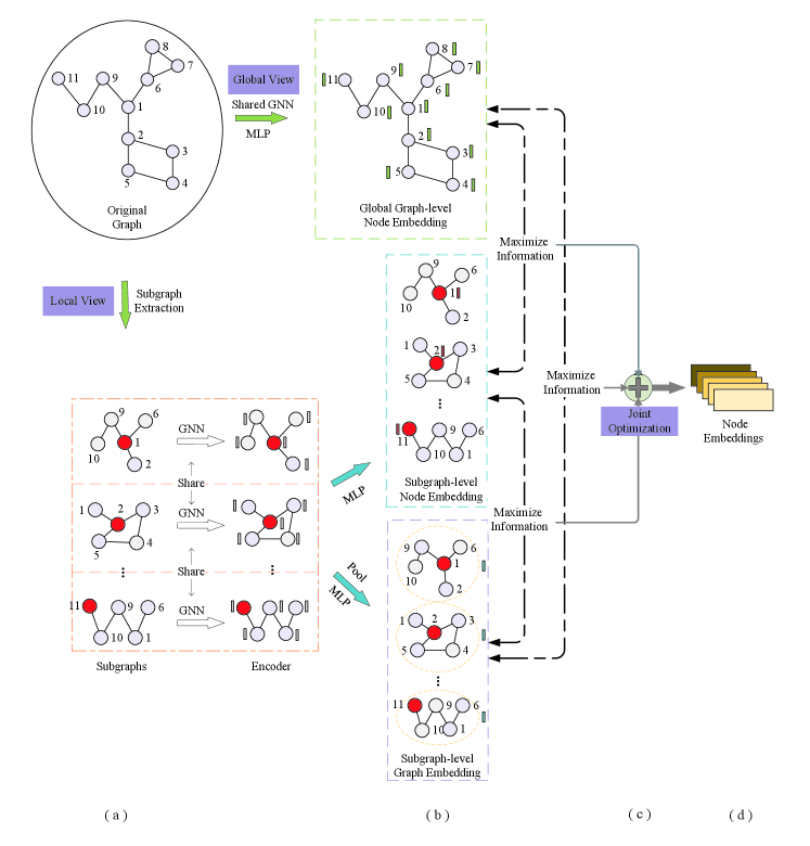
In the section, we introduce the Local Structure-aware Graph Contrastive representation Learning method (LS-GCL). The architecture of our LS-GCL is shown in the Fig.1.
2.1 Notations
Let indicates an undirected attributed graph, where and denote the set of nodes and edges, respectively. We denote the adjacency matrix of the graph and the initial feature matrix of the nodes as and , where N and F represent the number of nodes in the graph and the dimension of the initial attribute feature, respectively. if (, ) . denotes the initial feature of node .
2.2 Data Augmentation with Semantic Subgraph
In the GCL framework, the positive and negative samples for graph-structured data are constructed in terms of the graph structure or the attribute features of nodes, which affect the learning ability of the encoder[24]. The DGI obtains the corrupted graph by shuffling the node order of the feature matrix and utilizes the corrupted graph embedding and original graph embedding as negative sample and positive sample separately [18]. The GGD[25] obtains the corrupted graph by the edge and feature dropout, and assigns different manual labels to the nodes in the original graph and corrupted graph to train the GNN encoder[25]. However, global graph embedding, which compresses too much structural information into a simple fixed-length vector, approximates the constant vector[25], and the edge dropout methods ignore the information of the substructure.
In this paper, to explore the local graph structural information, we apply the semantic subgraph for data augmentation. Considering the structural information of nodes mainly depends on local neighbors, we introduce the personalized pagerank algorithm (PPR) [26], which searches for the top related nodes to target nodes, to construct the semantic subgraphs.
Given the adjacency matrix A of original graph , we firstly obtain the importance score matrix M, which is calculated as shown in Eq.1:
| (1) |
where is an optional parameter which is set as 0.15 and I denotes the identity matrix. represents the column-normalized adjacency matrix, where D indicates the diagonal matrix with . And denotes the importance score vector of node , where each value represents the relative importance between node and another node.
For the target node , we obtain the top important node set via the importance score vector of node . The calculation process is shown below:
| (2) |
where indicates the count of nodes in the semantic subgraph and is a function that returns the index of the top related nodes. We construct semantic subgraphs via the obtained nodes and the relationships between them:
| (3) |
where and denote the attribute information and structural information of the semantic subgraph for target node , respectively. The process of generating subgraphs can be achieved as a pre-task to reduce memory usage and running time compared to the online subgraph generation methods.
2.3 The contrastive objective
In the LS-GCL, each contrastive objective represents the local structural and semantic information of the target nodes in different levels. In this paper, we use a single GCN layer as the encoder to learn the node embeddings, and add a shared MLP layer for enhancing the expressiveness of the GNN encoder. The calculation process is as follows:
| (4) |
where and denotes the identity matrix. and W represents the weight matrix to be trained in the GNN encoder. denotes the activation function (PReLU). In our LS-GCL framework, the GNN encoder can be changed, such as the GAT, GraphSAGE and SGC which have different message aggregation methods.
For the semantic subgraph of target node , we employ the GNN-based encoder to learn the target node embeddings. The calculation process is as follows:
| (5) |
where represents the embedding of target node at the subgraph-level. The purpose of constructing semantic subgraph is to maximize the local structural information of nodes. Therefore, we apply a pooling function to generate the subgraph-level graph embedding for target node :
| (6) |
where is the pooling function and represents the embedding representation of the semantic subgraph for target node . In our experiments, we apply the mean-pooling function to learn the subgraph embeddings, which averages the feature vectors of nodes in the subgraph .
Furthermore, we add the target node embeddings from the global-graph view as the contrastive objective.
| (7) |
where represents the embedding representation of target node at global graph-level.
Finally, we obtain the structural information of target nodes from multiple perspectives, including the node embedding at the global graph-level, the node embedding at the subgraph-level and the corresponding subgraph-level graph embedding, which can explain the semantic information of nodes from different levels.
2.4 Multi-level Contrastive Learning Framework
In the paper, the process of LS-GCL is to define a pre-task that constructs positive and negative samples for training the GNN encoder without using label information. For the target node , the LS-GCL combines the node embedding at the global graph-level and the node embedding at subgraph-level as well as the subgraph-level graph embedding . The LS-GCL then adopts the margin triplet loss function[27] to train the GNN encoder. To reduce the training time of the LS-GCL model, we conduct contrastive learning for any two perspectives in parallel. The contrastive loss function between the node embeddings at subgraph-level and the subgraph-level graph embeddings for target node is as follows:
| (8) |
where denotes the sigmoid function. is the margin value. is the negative sample embedding where is one of the other nodes.
The contrastive loss function between the node embeddings at subgraph-level and the node embeddings at global graph-level for target node is as follows:
| (9) |
The contrastive loss function between the node embeddings at the global graph-level and subgraph-level graph embeddings for target node is as follows:
| (10) |
To capture the comprehensive structural and semantic information, the overall contrastive loss function of the proposed LS-GCL can be defined as follows:
| (11) |
We adopt the Adam optimizer to adjust the parameters of the GNN encoder through the back propagation mechanism for maximizing the common information of node embeddings at three levels. The pseudocode of the LS-GCL model is summarized in Algorithm 1.
3 Experiments and Results
In this section, we evaluate the effectiveness and robustness of the proposed LS-GCL model by the performances of node classification and link prediction experiments on five real-world datasets, and analyse the different components of the LS-GCL framework to identify their necessity.
3.1 Datasets
In the experiments, we utilize five public datasets, such as Cora[28], Citeseer[29], Pubmed[30], Cora_ML[31] and DBLP[32] datasets. The five datasets are the citation graphs, where nodes represent scientific papers and edges represent the citation relationships between papers. Each node in the datasets has the initial features and a unique category label. The statistical information of the five datasets is shown in Table 1.
| Datasets | Nodes | Edges | Features | Classes |
|---|---|---|---|---|
| Cora | 2708 | 5429 | 1433 | 7 |
| Cora_ML | 2995 | 8158 | 2876 | 7 |
| Citeseer | 3327 | 4732 | 3703 | 6 |
| DBLP | 17716 | 52867 | 1639 | 4 |
| Pubmed | 19717 | 44338 | 500 | 3 |
3.2 Baselines
For the tasks of node classification and link prediction, we use two classical semi-supervised learning algorithms and four state-of-art graph contrastive learning algorithms as baseline algorithms. For the baseline methods, we report their experimental results on downstream tasks based on their open codes.
-
1.
GCN: The graph convolutional network (GCN) is a classical graph neural network algorithm that captures the structural information of target nodes by aggregating the feature information of neighbors to learn the node embeddings. The training process requires the participation of label information.
-
2.
GAT: The graph attention network (GAT) is one of the classical graph neural network algorithms. It introduces the attention mechanism to aggregate the feature information of neighbors to extract the structural information of nodes. The training process of the GAT requires label information.
-
3.
DGI: The deep graph infomax (DGI) is an unsupervised learning model that maximizes the common information between the target nodes and the global graph by establishing a contrastive perspective between the node level and the global graph level to generate the node embedding representations.
-
4.
GMI: The graphical mutual information (GMI) is an unsupervised method that maximizes the mutual information of both features and edges between input graph and output graph of the encoder to learn node embeddings.
-
5.
SUBG-CON: The sub-graph contrast (SUBG-CON) is a self-supervised learning paradigm, which maximizes the common information at the node-level and subgraph-level by constructing the subgraphs for nodes. The SUBG-CON method alleviates the memory problem of the GCL paradigm.
-
6.
GGD: The graph group discrimination (GGD) is a self-supervised learning model, which trains the model by assigning different artificial labels to positive and negative samples to achieve the consistency of feature information between similar samples and then obtains the embedding representations of nodes.
3.3 Experimental Settings
In the experiments, for the graph , we employ the personalized pagerank (PPR) algorithm to obtain the top important node sets of target nodes for constructing the semantic subgraphs. We set on five datasets in the experiments. For the parameter in the margin triplet loss function, we set on the four datasets except that the value of in the Pubmed dataset is 0.35. In the GNN encoder, the input dimension is the initial feature dimension of the nodes, and the output dimension is 1000, except for 450 in the Pubmed dataset. We use the Adam optimizer with an initial learning rate of 0.001 to adjust the parameters of the encoder. The experiments are conducted on an eight-core Intel i7 2.50 GHz processor and 16 GB of RAM and a NVIDIA RTX 3090 24G GPUs.
3.4 Node Classification
Compared to supervised learning methods, the proposed LS-GCL model exploits structural feature information of nodes using known graph structures (e.g. adjacency matrices), without the node labels, to learn the node embeddings. We then use a small number of labels, such as 20 labels for each category of nodes, to fine-tune[33] the node embeddings for specific node classification task.
Experimental results of node classification in terms of accuracy on five real-world datasets are shown in Table 2. All experimental results are the mean and standard deviation of ten repeated node classification experiments. We can find that the proposed LS-GCL model obtains optimal node classification accuracy on all five datasets. Our LS-GCL model mines the semantic information of nodes from both local and global perspectives. Nodes with similar structural features in the graph generate similar node embeddings, which helps to predict the unknown labels of nodes. In addition, the node classification accuracy of the GCL models is higher than that of the semi-supervised learning methods on five datasets, demonstrating that the GCL methods are useful for capturing latent structural features of nodes.
| Methods | Available data | Cora | Citeseer | Pubmed | Cora_ML | DBLP |
|---|---|---|---|---|---|---|
| GCN | X, A, Y | 81.5±0.3 | 70.3±0.5 | 78.8±0.2 | 82.4±0.8 | 75.4±0.5 |
| GAT | X, A, Y | 82.9±0.7 | 71.8±0.7 | 79.2±0.3 | 84.6±0.7 | 74.2±0.4 |
| DGI | X, A | 81.3±0.5 | 71.6±0.5 | 77.7±0.5 | 80.6±0.2 | 78.3±0.3 |
| GMI | X, A | 82.6±0.2 | 69.2±0.4 | 78.2±0.6 | 81.7±0.4 | 78.6±0.6 |
| SUBG-CON | X, A | 83.5±0.5 | 72.7±0.6 | 79.9±0.4 | 84.3±0.1 | 80.3±0.5 |
| GGD | X, A | 83.8±0.4 | 72.8±0.8 | 80.9±0.5 | 83.1±0.9 | 80.8±0.3 |
| LS-GCL | X, A | 84.4±0.4 | 73.0±0.3 | 81.5±0.6 | 86.9±0.5 | 80.9±0.4 |
3.5 Link Prediction
The task of link prediction is to predict potential node-pair relationships according to the structural features between nodes in the graph. Traditional GNN models, which are the supervised learning methods, require a large number of labels to train the parameters of the model for capturing the relationships between node pairs for link prediction experiments[34]. The LS-GCL learns target node embeddings in the link prediction task is similar with the node classification experiments. Our model migrates the node embeddings obtained from pre-training process to the downstream tasks by fine-tuning. The link embeddings are generated by concatenating the embedding vectors of the node pairs. The training and test sets containing positive and negative samples as well as the corresponding link labels are fed into a classifier (e.g. random forest[35]) to evaluate the effectiveness of the node embeddings generated by the LS-GCL model. In the five datasets, the proportion of test set is 40%.
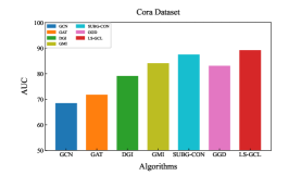
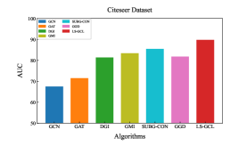
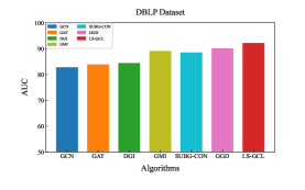
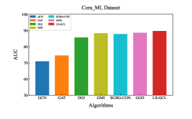
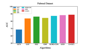
Experimental results of link prediction for the AUC index on five real-world datasets are shown in the Fig. 2. To illustrate the robustness of the proposed LS-GCL, we use three other metrics, namely Recall, Precision and F1-score(F1)[36], which are shown in Table 3 and Table 4. All experimental results are the mean and standard deviation of ten repeated link prediction experiments. We can see that our LS-GCL model achieves outstanding and stable experimental results on four evaluation indices for all five datasets compared to current GCL and semi-supervised learning models. The node embeddings obtained by the GCL method with fine-tuning achieve an improvement in the link prediction task compared to the traditional GNN model.
| Methods | Cora | Citeseer | Pubmed | ||||||
|---|---|---|---|---|---|---|---|---|---|
| Recall | Precision | F1 | Recall | Precision | F1 | Recall | Precision | F1 | |
| GCN | 56.9±0.2 | 74.2±0.4 | 65.7±0.3 | 52.8±0.3 | 75.6±0.2 | 61.4±0.4 | 64.4±0.3 | 70.3±0.1 | 67.2±0.1 |
| GAT | 50.4±0.2 | 88.7±0.3 | 64.1±0.5 | 51.9±0.5 | 87.2±0.6 | 67.4±0.4 | 72.5±0.4 | 85.3±0.5 | 81.4±0.3 |
| DGI | 73.0±0.6 | 83.1±0.8 | 77.7±0.3 | 69.6±0.5 | 91.1±0.3 | 78.9±0.4 | 84.0±0.9 | 88.1±0.9 | 85.9±0.6 |
| GMI | 74.1±0.3 | 92.6±0.3 | 82.3±0.2 | 69.9±0.5 | 95.8±0.1 | 80.9±0.4 | 80.6±0.2 | 87.3±0.7 | 83.8±0.6 |
| SUBG-CON | 86.3±0.5 | 88.4±0.5 | 87.3±0.4 | 82.7±0.6 | 87.6±0.4 | 85.1±0.4 | 87.6±0.6 | 86.8±0.1 | 87.2±0.6 |
| GGD | 73.4±0.8 | 91.1±0.4 | 81.3±0.6 | 70.9±0.9 | 90.8±0.6 | 79.6±0.5 | 85.0±0.7 | 90.2±0.9 | 87.8±0.5 |
| LS-GCL | 88.7±0.2 | 91.6±0.4 | 88.9±0.3 | 90.4±0.1 | 90.2±0.2 | 88.8±0.4 | 90.7±0.3 | 88.2±0.1 | 88.3±0.4 |
| Methods | Cora_ML | DBLP | ||||
|---|---|---|---|---|---|---|
| Recall | Precision | F1 | Recall | Precision | F1 | |
| GCN | 68.5±0.5 | 72.5±0.4 | 69.1±0.2 | 73.2±0.1 | 88.7±0.6 | 81.5±0.3 |
| GAT | 69.6±0.5 | 79.1±0.3 | 72.8±0.5 | 75.5±0.3 | 91.7±0.2 | 82.6±0.4 |
| DGI | 81.1±0.4 | 89.4±0.4 | 85.0±0.3 | 82.3±0.2 | 86.0±0.7 | 84.1±0.1 |
| GMI | 83.2±0.3 | 92.6±0.2 | 87.7±0.1 | 86.2±0.5 | 91.4±0.2 | 88.7±0.4 |
| SUBG-CON | 84.4±0.4 | 90.5±0.3 | 87.3±0.2 | 89.6±0.1 | 87.7±0.9 | 88.6±0.9 |
| GGD | 84.5±0.3 | 92.1±0.3 | 88.1±0.2 | 87.9±0.1 | 93.0±0.6 | 90.9±0.1 |
| LS-GCL | 86.7±0.2 | 94.5±0.5 | 89.4±0.3 | 93.1±0.2 | 93.4±0.1 | 92.2±0.5 |
4 Ablation Study
4.1 Analysis of Subgraph Extraction Methods
The LS-GCL model has achieved better results in both node classification and link prediction tasks. In this section, we discuss three different ways of constructing subgraphs to evaluate the effectiveness of semantic subgraphs and the robustness of our LS-GCL framework. -hop subgraph[37] represents that the subgraphs are constructed by the neighboring nodes which are hop away from the target nodes. We construct the 1-hop subgraphs to capture the local structural features of target nodes. -RW subgraph denotes that the local subgraphs are constructed by the path generated through the random walk algorithm with length for the target nodes. We set the length of the random walk as 20 to obtain the same size subgraph. -rank subgraph denotes the semantic subgraph which contains top related nodes.
Node classification results of three methods for extracting subgraphs are shown in Table 5. Our LS-GCL method with semantic subgraphs has higher accuracy than the LS-GCL model based on -hop subgraphs and -RW subgraphs, which indicates that the semantic subgraphs are capable for capturing potential structural information of nodes. The semantic subgraphs not only focus on the first-order neighboring nodes of target nodes, but also consider the higher-order related nodes, which enriches the semantic information of nodes.
| Cora | Citeseer | Pubmed | Cora_ML | DBLP | |
|---|---|---|---|---|---|
| K-hop | 79.4±0.5 | 71.2±0.3 | 78.5±0.6 | 82.6±0.3 | 77.3±0.4 |
| K-RW | 79.1±0.6 | 71.1±0.4 | 80.2±0.5 | 81.6±0.7 | 76.1±0.8 |
| K-rank | 84.4±0.4 | 73.0±0.3 | 81.5±0.6 | 86.9±0.5 | 80.9±0.4 |
4.2 Analysis of Subgraph Size
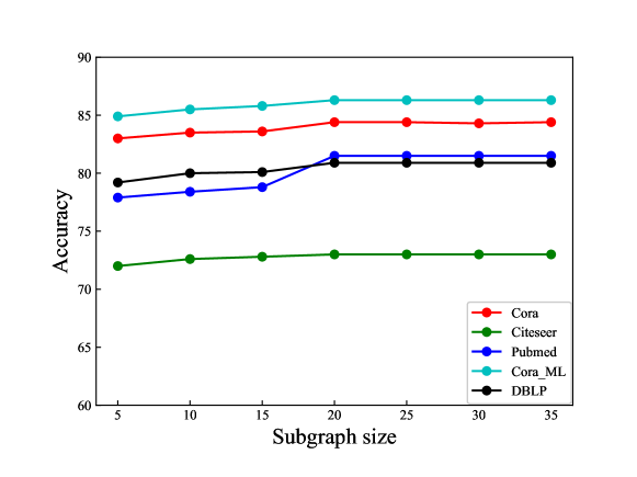
The semantic subgraphs of our LS-GCL model are constructed with the top relevant nodes. We investigate how subgraph size affects the actual performance of our model on node classification task, which is shown in the Fig.3. It has been shown that the node classification accuracy of the LS-GCL model steadily improves as the subgraph size increases. For the five datasets, the accuracy gradually improves as the subgraph size increases from 0 to 20, indicating that GNN can extract more structural information from semantic subgraphs with more nodes. The node classification accuracy of the LS-GCL model reaches a plateau when the number of nodes exceeds 20. Compared to traditional GCL methods such as the SUBG-CON, the LS-GCL model considers the global graph structure, which improves the robustness of our model in downstream tasks.
4.3 Analysis of Encoder
In this paper, the proposed LS-GCL uses the GNN model as an encoder to learn node embeddings. We perform node classification experiments with different GNN models as feature encoders to test the impact of the encoders on our LS-GCL framework. For the GAT, the GraphSAGE[38], the SGC model[39], we apply a single GNN layer as the encoders. The experimental results are shown in Table 6. Our LS-GCL framework using a GCN-based encoder achieves higher accuracy on four datasets except the DBLP dataset. The node classification accuracy of the GNN-based encoders varies slightly between the five datasets, which demonstrates that our LS-GCL framework is robust. We can adapt the different GNN encoders to the actual situation and design a specific LS-GCL model for the downstream tasks.
| Cora | Citeseer | pubmed | Cora_ML | DBLP | |
|---|---|---|---|---|---|
| GCN | 84.4±0.4 | 73.0±0.3 | 81.5±0.6 | 86.9±0.5 | 80.9±0.4 |
| GAT | 82.6±0.5 | 72.6±0.9 | 80.3±0.7 | 86.5±0.6 | 81.3±0.9 |
| GraphSAGE | 84.0±0.5 | 72.1±0.7 | 79.4±0.2 | 86.1±0.4 | 79.1±0.2 |
| SGC | 84.1±0.4 | 72.6±0.6 | 80.5±0.9 | 86.8±0.6 | 79.7±0.3 |
4.4 Analysis of Contrastive Loss Function
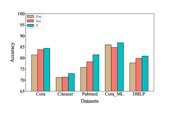
In the paper, we propose a new multi-level contrastive loss function . To reflect the semantic information of nodes at different levels, we set the node embeddings at the global graph-level, the node embeddings at the subgraph-level and the subgraph-level graph embeddings corresponding to target nodes as the contrastive objectives. To evaluate the effectiveness of the multi-level contrastive loss function, we use and as the contrastive loss functions to learn the target node embeddings and perform node classification experiments, respectively. denotes that the contrastive objectives are node embeddings at subgraph-level and global graph-level. denotes that the contrastive objectives are node embeddings at subgraph-level and subgraph-level graph embeddings corresponding to target nodes. Experimental results of node classification experiments corresponding to different contrastive loss functions on five datasets are shown in Fig.4. The LS-GCL model using the multi-level contrastive loss function achieves better results than and . Compared with the models using and as the contrastive loss functions, the LS-GCL model captures different semantic information at three levels and each contrastive object has an essential role in the maximisation of the feature information for target nodes.
5 Conclusion and Discussions
In the paper, we propose a novel GCL framework named LS-GCL that pays attention to local structural information of nodes at multiple levels. To capture more local structural information, we construct semantic subgraphs for nodes by the PPR algorithm. A shared GNN-based encoder is employed to mine the structural information of the local semantic subgraphs for target nodes. We obtain the target node embeddings at the subgraph-level and subgraph embeddings corresponding to target nodes to capture local structural features at different levels. To preserve the potential semantic information of the original graph, we learn the target node embedding at the global graph-level. Finally, we construct a multi-level contrastive loss function to maximize the common information of target nodes at different levels and obtain the final node embeddings. We conduct node classification and link prediction experiments on various real-world datasets and achieve superior performance comparing with classical GNN and GCL models.
The proposed LS-GCL model requires numerous iterations to learn the parameters of encoder, which uses more running memory than traditional GNN models. How to alleviate the memory and time limitations of LS-GCL model is a public problem. In addition, we aim to extend the LS-GCL framework to the heterogeneous information graphs that contain multiple types of nodes or relations[40]. The semantic subgraph proposed in our model will contribute to the mining of potential semantic information in heterogeneous graphs. In the future, the LS-GCL framework will be proposed to apply on the homogeneous graphs and heterogeneous graphs.
6 Acknowledgments
This work is supported in part by the Natural Science Foundation of the Jiangsu Higher Education Institutions of China(No.22KJD120002).
References
- [1] W. Fan, Y. Ma, Q. Li, Y. He, E. Zhao, J. Tang, D. Yin, Graph neural networks for social recommendation, in: The World Wide Web Conference, 2019, pp. 417–426.
- [2] N. A. Asif, Y. Sarker, R. K. Chakrabortty, M. J. Ryan, M. H. Ahamed, D. K. Saha, F. R. Badal, S. K. Das, M. F. Ali, S. I. Moyeen, M. R. Islam, Z. Tasneem, Graph neural network: A comprehensive review on non-euclidean space, IEEE Access 9 (2021) 60588–60606.
- [3] Z. Wu, S. Pan, F. Chen, G. Long, C. Zhang, S. Y. Philip, A comprehensive survey on graph neural networks, IEEE Transactions on Neural Networks and Learning Systems 32 (1) (2020) 4–24.
- [4] T. N. Kipf, M. Welling, Semi-supervised classification with graph convolutional networks, arXiv preprint arXiv:1609.02907 (2016).
- [5] P. Veličković, G. Cucurull, A. Casanova, A. Romero, P. Lio, Y. Bengio, Graph attention networks, arXiv preprint arXiv:1710.10903 (2017).
- [6] S. Wu, F. Sun, W. Zhang, X. Xie, B. Cui, Graph neural networks in recommender systems: a survey, ACM Computing Surveys 55 (5) (2022) 1–37.
- [7] F. Zhou, Q. Yang, T. Zhong, D. Chen, N. Zhang, Variational graph neural networks for road traffic prediction in intelligent transportation systems, IEEE Transactions on Industrial Informatics 17 (4) (2020) 2802–2812.
- [8] T. Nguyen, H. Le, T. P. Quinn, T. Nguyen, T. D. Le, S. Venkatesh, Graphdta: predicting drug–target binding affinity with graph neural networks, Bioinformatics 37 (8) (2021) 1140–1147.
- [9] T. Chen, X. Zhang, M. You, G. Zheng, S. Lambotharan, A gnn-based supervised learning framework for resource allocation in wireless iot networks, IEEE Internet of Things Journal 9 (3) (2021) 1712–1724.
- [10] Z. Song, X. Yang, Z. Xu, I. King, Graph-based semi-supervised learning: A comprehensive review, IEEE Transactions on Neural Networks and Learning Systems (2022) 1–21.
- [11] B. Wu, Y. Bian, H. Zhang, J. Li, J. Yu, L. Chen, C. Chen, J. Huang, Trustworthy graph learning: Reliability, explainability, and privacy protection, in: Proceedings of the 28th ACM SIGKDD Conference on Knowledge Discovery and Data Mining, 2022, pp. 4838–4839.
- [12] N. Yin, Z. Luo, Generic structure extraction with bi-level optimization for graph structure learning, Entropy 24 (9) (2022) 1228.
- [13] C. Tao, H. Wang, X. Zhu, J. Dong, S. Song, G. Huang, J. Dai, Exploring the equivalence of siamese self-supervised learning via a unified gradient framework, in: Proceedings of the IEEE/CVF Conference on Computer Vision and Pattern Recognition, 2022, pp. 14431–14440.
- [14] W. Jin, T. Derr, H. Liu, Y. Wang, S. Wang, Z. Liu, J. Tang, Self-supervised learning on graphs: Deep insights and new direction, arXiv preprint arXiv:2006.10141 (2020).
- [15] S. Xiao, S. Wang, Y. Dai, W. Guo, Graph neural networks in node classification: survey and evaluation, Machine Vision and Applications 33 (2022) 1–19.
- [16] Egc2: Enhanced graph classification with easy graph compression, Information Sciences 629 (2023) 376–397.
- [17] A. Rossi, D. Barbosa, D. Firmani, A. Matinata, P. Merialdo, Knowledge graph embedding for link prediction: A comparative analysis, ACM Transactions on Knowledge Discovery from Data (TKDD) 15 (2) (2021) 1–49.
- [18] P. Veličković, W. Fedus, W. L. Hamilton, P. Liò, Y. Bengio, R. D. Hjelm, Deep graph infomax, arXiv preprint arXiv:1809.10341 (2018).
- [19] Y. Zhu, Y. Xu, F. Yu, Q. Liu, S. Wu, L. Wang, Deep graph contrastive representation learning, arXiv preprint arXiv:2006.04131 (2020).
- [20] Y. Zhu, Y. Xu, F. Yu, Q. Liu, S. Wu, L. Wang, Graph contrastive learning with adaptive augmentation, in: Proceedings of the Web Conference, 2021, pp. 2069–2080.
- [21] Z. Peng, W. Huang, M. Luo, Q. Zheng, Y. Rong, T. Xu, J. Huang, Graph representation learning via graphical mutual information maximization, in: Proceedings of The Web Conference, 2020, pp. 259–270.
- [22] K. Hassani, A. H. Khasahmadi, Contrastive multi-view representation learning on graphs, in: International Conference on Machine Learning, 2020, pp. 4116–4126.
- [23] Y. Jiao, Y. Xiong, J. Zhang, Y. Zhang, T. Zhang, Y. Zhu, Sub-graph contrast for scalable self-supervised graph representation learning, in: IEEE International Conference on Data Mining (ICDM), 2020, pp. 222–231.
- [24] S. Feng, B. Jing, Y. Zhu, H. Tong, Adversarial graph contrastive learning with information regularization, in: Proceedings of the ACM Web Conference 2022, 2022, pp. 1362–1371.
- [25] Y. Zheng, S. Pan, V. C. Lee, Y. Zheng, P. S. Yu, Rethinking and scaling up graph contrastive learning: An extremely efficient approach with group discrimination, arXiv preprint arXiv:2206.01535 (2022).
- [26] H. Wang, Z. Wei, J. Gan, S. Wang, Z. Huang, Personalized pagerank to a target node, revisited, in: Proceedings of the 26th ACM SIGKDD International Conference on Knowledge Discovery & Data Mining, 2020, pp. 657–667.
- [27] M. L. Ha, V. Blanz, Deep ranking with adaptive margin triplet loss, arXiv preprint arXiv:2107.06187 (2021).
- [28] Y. Chen, J. You, J. He, Y. Lin, Y. Peng, C. Wu, Y. Zhu, Sp-gnn: Learning structure and position information from graphs, Neural Networks 161 (2023) 505–514.
- [29] T. Tian, L. Zhao, X. Wang, Q. Wu, W. Yuan, X. Jin, Fp-gnn: Adaptive fpga accelerator for graph neural networks, Future Generation Computer Systems 136 (2022) 294–310.
- [30] Z. Zhou, J. Shi, S. Zhang, Z. Huang, Q. Li, Effective stabilized self-training on few-labeled graph data, Information Sciences (2023).
- [31] S. Geisler, D. Zügner, S. Günnemann, Reliable graph neural networks via robust aggregation, Advances in Neural Information Processing Systems 33 (2020) 13272–13284.
- [32] Z. Tong, Y. Liang, C. Sun, D. S. Rosenblum, A. Lim, Directed graph convolutional network, arXiv preprint arXiv:2004.13970 (2020).
- [33] P. Wang, K. Agarwal, C. Ham, S. Choudhury, C. K. Reddy, Self-supervised learning of contextual embeddings for link prediction in heterogeneous networks, in: Proceedings of the Web Conference, 2021, pp. 2946–2957.
- [34] K. Yang, Y. Liu, Z. Zhao, X. Zhou, P. Ding, Graph attention network via node similarity for link prediction, The European Physical Journal B 96 (3) (2023) 27.
- [35] S. J. Rigatti, Random forest, Journal of Insurance Medicine 47 (1) (2017) 31–39.
- [36] R. Yacouby, D. Axman, Probabilistic extension of precision, recall, and f1 score for more thorough evaluation of classification models, in: Proceedings of the First Workshop on Evaluation and Comparison of NLP Systems, 2020, pp. 79–91.
- [37] Y. Duan, J. Wang, H. Ma, Y. Sun, Residual convolutional graph neural network with subgraph attention pooling, Tsinghua Science and Technology 27 (4) (2021) 653–663.
- [38] W. Hamilton, Z. Ying, J. Leskovec, Inductive representation learning on large graphs, Advances in neural information processing systems 30 (2017).
- [39] F. Wu, A. Souza, T. Zhang, C. Fifty, T. Yu, K. Weinberger, Simplifying graph convolutional networks, in: International Conference on Machine Learning, PMLR, 2019, pp. 6861–6871.
- [40] S. Zhu, C. Zhou, A. Cheng, S. Pan, S. Wang, D. Yin, B. Wang, Geometry contrastive learning on heterogeneous graphs, arXiv preprint arXiv:2206.12547 (2022).