Localized active learning of Gaussian process state space models
Abstract
While most dynamic system exploration techniques aim to achieve a globally accurate model, this is generally unsuited for systems with unbounded state spaces. Furthermore, many applications do not require a globally accurate model, e.g., local stabilization tasks. In this paper, we propose an active learning strategy for Gaussian process state space models that aims to obtain an accurate model on a bounded subset of the state-action space. Our approach aims to maximize the mutual information of the exploration trajectories with respect to a discretization of the region of interest. By employing model predictive control, the proposed technique integrates information collected during exploration and adaptively improves its exploration strategy. To enable computational tractability, we decouple the choice of most informative data points from the model predictive control optimization step. This yields two optimization problems that can be solved in parallel. We apply the proposed method to explore the state space of various dynamical systems and compare our approach to a commonly used entropy-based exploration strategy. In all experiments, our method yields a better model within the region of interest than the entropy-based method.
keywords:
exploration, Bayesian inference, data-driven control, model predictive control1 Introduction
Autonomous systems often need to operate in complex environments, of which a model is difficult or even impossible to derive from first principles. Learning-based techniques have become a promising paradigm to address these issues (Pillonetto et al., 2014). In particular, Gaussian processes (GPs) have been increasingly employed for system identification and control (Umlauft et al., 2018; Capone and Hirche, 2019; Berkenkamp and Schoellig, 2015; Deisenroth et al., 2015). GPs possess very good generalization properties (Rasmussen and Williams, 2006), which can be leveraged to obtain data-efficient learning-based approaches (Deisenroth et al., 2015; Kamthe and Deisenroth, 2018). By employing a Bayesian framework, GPs provide an automatic trade-off between model smoothness and data fitness. Moreover, GPs provide an explicit estimate of the model uncertainty that is used to derive probabilistic bounds in control settings (Capone and Hirche, 2019; Beckers et al., 2019; Umlauft and Hirche, 2020).
A performance-determining factor of data-driven techniques is the quality of the available data. In settings where data is insufficient to achieve accurate predictions, new data needs to be gathered via exploration (Umlauft and Hirche, 2020). In classical reinforcement learning settings, exploration is often enforced by randomly selecting a control action with a predetermined probability that tends to zero over time (Dayan and Sejnowski, 1996). However, this is generally inefficient, as regions of low uncertainty are potentially revisited in multiple iterations. These issues have been addressed by techniques that choose the most informative exploration trajectories (Alpcan and Shames, 2015; Ay et al., 2008; Burgard et al., 2005; Schreiter et al., 2015). The goal of these methods is to obtain a globally accurate model. While this is reasonable for systems with a bounded state-action space, it is unsuited for systems with unbounded ones, particularly if a non-parametric model is used. This is because a potentially infinite number of points is required to achieve a globally accurate model. Furthermore, in practice a model often only needs to be accurate locally, e.g., for stabilization tasks.
In this paper, we propose a model predictive control-based exploration approach that steers the system towards the most informative points within a bounded subset of the state-action space. By modeling the system with a Gaussian process, we are able to quantify the information inherent in each data point. Our approach chooses actions by approximating the mutual information of the system trajectory with respect to a discretization of the region of interest. This is achieved by first selecting the single most informative data point within the region of interest, then steering the system towards that point using model predictive control. Through this approximation, the solution approach is rendered computationally tractable.
2 Problem Statement
We consider the problem of exploring the state and control space of a discrete-time nonlinear system with Markovian dynamics of the form
| (1) |
where , and are the system’s state vector and control vector at the -th time step, respectively. The system is disturbed by multivariate Gaussian process noise with , . The concatenation , where is employed for simplicity of exposition. The nonlinear function represents the known component of the system dynamics, e.g., a model obtained using first principles, while corresponds to the unknown component of the system dynamics.
We aim to obtain an approximation of the function , denoted , which provides an accurate estimate of on a predefined bounded subset of the augmented state space . This is often required in practice, e.g., for local stabilization tasks.
3 Gaussian Processes
In order to faithfully capture the stochastic behavior of (1), we model the system as a Gaussian process (GP), where we employ measurements of the augmented state vector as training inputs, and the differences as training targets.
A GP is a collection of dependent random variables variables, for which any finite subset is jointly normally distributed (Rasmussen and Williams, 2006). It is specified by a mean function and a positive definite covariance function , also known as kernel. In this paper, we set without loss of generality, as all prior knowledge is already encoded in . The kernel is a similarity measure for evaluations of , and encodes function properties such as smoothness and periodicity.
In the case where the state is a scalar, i.e., , given training input samples and training outputs , the posterior mean and variance of the GP corresponds to a one-step transition model. Starting at a point , the difference between the subsequent state and the known component is normally distributed, i.e.,
| (2) |
with mean and variance given by
respectively, where , and the entries of the covariance matrix are computed as , .
In the case where the state is multidimensional, we model dimension of the state transition function using a separate GP. This corresponds to the assumption that the state transition function entries are conditionally independent. For simplicity of exposition, unless stated otherwise, we henceforth assume . However, the methods presented in this paper extend straightforwardly to the multivariate case.
3.1 Performing multi-step ahead predictions
The GP model presented in the previous section serves as a one-step predictor given a known test input . However, if only a distribution is available, the successor states’ distribution generally cannot be computed analytically. Hence, the distributions of future states cannot be computed exactly, but only approximated, e.g., using Monte Carlo methods (Candela et al., 2003). Alternatively, approximate computations exist that enable to propagate the GP uncertainty over multiple time steps, such as moment-matching and GP linearization (Deisenroth et al., 2015). In this paper, we employ the GP mean to perform multi-step ahead predictions, without propagating uncertainty, i.e., , . However, the proposed method is also applicable using models that propagate uncertainty, e.g., moment-matching (Deisenroth et al., 2015).
3.2 Quantifying utility of data
In order to steer the system along informative trajectories, we need to quantify the utility of data points in the augmented state space . To this end, we consider the mutual information between observations at training inputs and evaluations at reference points . Here is a discretization of the bounded subset . Formally, the mutual information between and is given by
| (3) |
respectively denote the differential entropy of and the conditional differential entropy of given . In practice, computing (3) for a multi-step GP prediction is intractable. However, we can obtain the single most informative data point with respect to by computing the unconstrained minimum of
| (4) |
where denotes the determinant of a square matrix. In settings with unconstrained decision spaces, sequentially computing a minimizer of (4) has been shown to yield a solution that corresponds to at least of the optimal value (Krause et al., 2008).
4 The LocAL algorithm
| s.t. |
The system dynamics (1) considerably limit the decision space at every time step . Furthermore, after a data point is collected, both the GP model and mutual information change. Hence, we employ a model predictive control (MPC)-based approach to steer the system towards areas of high information. Ideally, at every MPC-step , we would like to minimize (3) with respect to a series of inputs . However, this is generally infeasible, limiting its applicability in an MPC setting. Hence, we consider an approximate solution approach that sequentially computes the most informative data point by minimizing (4) separately from the MPC optimization. This is achieved as follows. At every time step , an unconstrained minimizer of (4) is computed. Afterwards, the MPC computes the approximate optimal inputs by minimizing a constrained optimization problem that penalizes the weighted distance to the reference point using a positive semi-definite weight matrix . The ensuing state is then measured, the GP model is updated, and the procedure is repeated. These steps yield the Localized Active Learning (LocAL) algorithm, which is presented in Algorithm 1.
The square weight matrix should be chosen such that the MPC steers the system as close to as possible. This represents a system-dependent task. Alternatively, can be chosen such that the MPC cost function corresponds to a quadratic approximation of the mutual information, e.g., such that holds for .
4.1 Sensitivity analysis
We now provide a sensitivity analysis of (4). Specifically, we show that the difference in mutual information at and is lower bounded. To this end, we require the following assumption.
Assumption 1
The kernel is Lipschitz continuous and upper bounded by .
This assumption holds for many commonly used kernels, e.g., the squared exponential kernel.
Using 1, we are able to bound the difference in mutual information at and an arbitrary state , as detailed in the following.
Theorem 4.1.
Let be the difference between the augmented state and the most informative data point at time step . Moreover, let denote the corresponding difference in mutual information, and let 1 hold. Then, there exists a constant , such that holds, where .
To prove Theorem 4.1, we require the following preliminary results.
Lemma 4.10.
For any , let denote the subset containing the first elements of . Then
| (5) | ||||
where denotes the posterior GP variance evaluated at conditioned on training data observed at .
Proof 4.14.
Hence, we employ the objective function
| (8) | ||||
with
| (9) |
Proof 4.15.
This follows directly from the property and Lemma 4.10.
Lemma 4.16.
Let be the covariance matrix used to compute , and let denote the matrix of partial derivatives of with respect to the -th entry of the -th data point . Then holds, where denotes the maximal eigenvalue.
Proof 4.21.
The matrix of partial derivatives has a single nonzero column and a single nonzero row. Its entries are
| (10) |
and its eigenvalues are given by
Corollary 4.26.
Let 1 hold. Then for a fixed set of data points the posterior covariance is Lipschitz continuous with respect to the data, with Lipschitz constant given by .
Proof 4.27.
For an arbitrary , data point , and corresponding entry ,
Here we employ the identities
| (11) |
and
| (12) |
where the latter identity follows from the positivity of .
We can now prove Theorem 4.1
Proof of Theorem 1
In particular, Theorem 4.1 implies that the mutual information with respect to can be approximated arbitrarily accurately by reducing the difference . In many control applications, this can be achieved in spite of the model error, e.g., by increasing control gains Capone and Hirche (2019); Umlauft and Hirche (2020). Hence, Theorem 4.1 can be potentially employed to guarantee a gradual improvement in model accuracy, or even to derive the worst-case number of iterations required to learn the system.
5 Numerical Experiments
In this section, we apply the proposed algorithm to four different dynamical systems. We begin with a toy example, with which we can easily illustrate the explored portions of the state space. Afterwards, we apply the proposed approach to a pendulum, a cart-pole, and a synthetic model that generalizes the mountain car problem. The exploration is repeated times for each system using different starting points sampled from a normal distribution. To quantify the performance of each approach, we compute the root mean square model error (RMSE) on points sampled from a uniform distribution on the region of interest .
We employ a squared-exponential kernel in all examples, and train the hyperparemters online using gradient-based log likelihood maximization (Rasmussen and Williams, 2006). We employ an MPC horizon of , and choose weight matrix for the MPC optimization step as
where denotes the standard deviation of the GP kernel corresponding to the -th dimension, and denote the corresponding lengthscales. In order to ease the computational burden, we apply the first inputs computed by the LocAL algorithm before computing a new solution.
We additionally explore each system using a greedy entropy-based cost function, as suggested in Koller et al. (2018) and Schreiter et al. (2015), and compare the results. In all three cases, the LocAL algorithm yields a better model in the regions of interest than the entropy-based algorithm.
5.1 Toy Problem
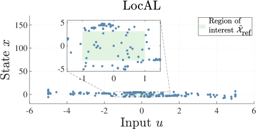
Consider the continuous-time nonlinear dynamical system
| (14) |
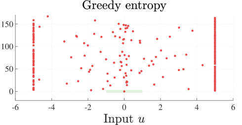
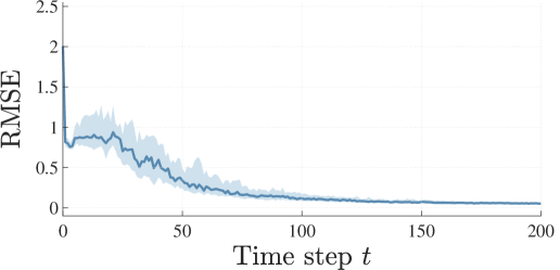
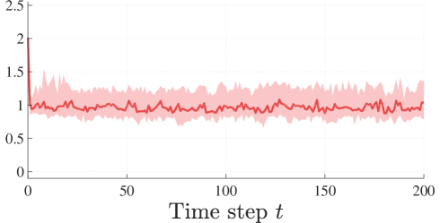
with state space and input space . We are interested in obtaining an accurate dynamical model within the region . To obtain a discrete-time system in the form of (1), we discretize (14) with a discretization step of and set the prior model to . The results are displayed in Figure 1.
The LocAL algorithm yields a substantial improvement in model accuracy in every run. This is because the system stays close to the region of interest during the whole simulation. By contrast, the greedy entropy-based method covers a considerably more extensive portion of the state space. This comes at the cost of a poorer model on , as indicated by the respective RMSE.
5.2 Surface exploration
We apply the LocAL algorithm to the dynamical system given by
| (15) |
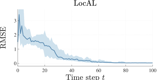
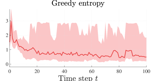
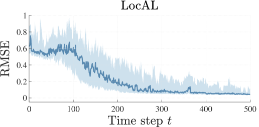
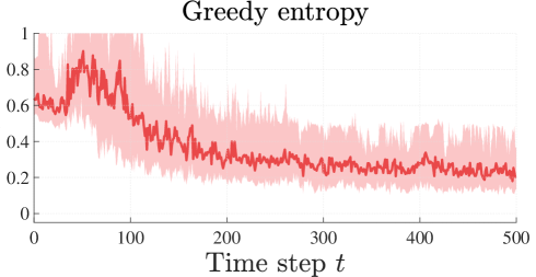
This setting can be seen as a surface exploration problem, i.e., an agent navigates a surface to learn its curvature. We aim to obtain an accurate model of the dynamics within the region given by . To run the LocAL algorithm, we employ a discretization step of and set the prior model to . The results are shown in Figure 2.
The LocAL algorithm manages to significantly improve its model after time steps, while the entropy-based strategy does not yield any improvement. This is because every variable of the state space is unbounded, i.e., the state space can be explored for a potentially infinite amount of time without ever reaching the region of interest .
5.3 Pendulum
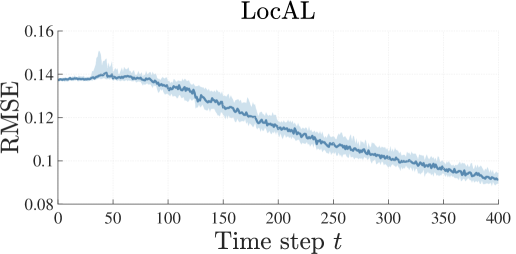
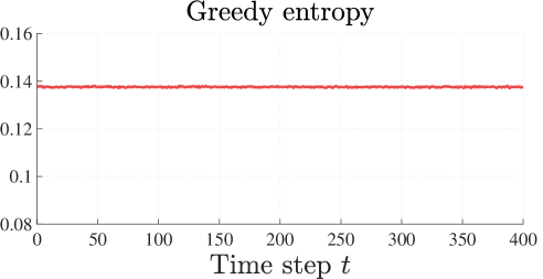
We now consider a two-dimensional pendulum, whose state is given by the angle and angular velocity . The input torque is constrained to the interval . Our goal is to obtain a suitable model within . Obtaining a precise model around this region is particularly useful for the commonly considered task of stabilizing the pendulum around the upward position . The results are depicted in Figure 3.
The RMSE indicates that the LocAL algorithm yields a similar model improvement every run. The model obtained with the entropy-based strategy, by contrast, exhibits higher errors.
5.4 Cart-pole
We apply the LocAL algorithm to the cart-pole system (Barto et al., 1983). The state space is given by , where is the cart velocity, is the pendulum angle, and is its angular velocity. Here we ignore the cart position, as it has no influence on the system dynamics. The region of interest is given by Similarly to the pendulum case, obtaining an accurate model on this region is useful to address the balancing task. The discretization step is set to , the prior model is . The results are shown in Figure 4.
Similarly to the pendulum case, the model obtained with the LocAL algorithm exhibits low standard deviation compared to the one obtained with the entropy-based approach. This is because the region of interest is explored more thoroughly with our approach.
6 Conclusion
A technique for efficiently exploring bounded subsets of the state-action space of a system has been presented. The proposed technique aims to minimize the mutual information of the system trajectories with respect to a discretization of the region of interest. It employs Gaussian processes both to model the unknown system dynamics and to quantify the informativeness of potentially collected data points. In numerical simulations of four different dynamical systems, we have demonstrated that the proposed approach yields a better model after a limited amount of time steps than a greedy entropy-based approach.
Acknowledgements
This work was supported by the European Research Council (ERC) Consolidator Grant ”Safe data-driven control for human-centric systems (CO-MAN)” under grant agreement number 864686 .
References
- Alpcan and Shames (2015) T. Alpcan and I. Shames. An information-based learning approach to dual control. IEEE transactions on neural networks and learning systems, 26(11):2736–2748, 2015.
- Ay et al. (2008) N. Ay, N. Bertschinger, R. Der, F. Güttler, and E. Olbrich. Predictive information and explorative behavior of autonomous robots. The European Physical Journal B, 63(3):329–339, 2008.
- Barto et al. (1983) A. G. Barto, R. S. Sutton, and C. W. Anderson. Neuronlike adaptive elements that can solve difficult learning control problems. IEEE Transactions on Systems, Man, and Cybernetics, SMC-13(5):834–846, 1983.
- Beckers et al. (2019) T. Beckers, D. Kulić, and S. Hirche. Stable Gaussian process based tracking control of euler-lagrange systems. Automatica, (103):390–397, 2019.
- Berkenkamp and Schoellig (2015) F. Berkenkamp and A. P. Schoellig. Safe and robust learning control with Gaussian processes. In Control Conference (ECC), 2015 European, pages 2496–2501. IEEE, 2015.
- Burgard et al. (2005) W. Burgard, D. Fox, and S. Thrun. Probabilistic robotics. The MIT Press, 2005.
- Candela et al. (2003) J. Q. Candela, A. Girard, J. Larsen, and C. E. Rasmussen. Propagation of uncertainty in Bayesian kernel models - application to multiple-step ahead forecasting. In 2003 IEEE International Conference on Acoustics, Speech, and Signal Processing, 2003. Proceedings. (ICASSP ’03)., volume 2, pages II–701, April 2003.
- Capone and Hirche (2019) A. Capone and S. Hirche. Backstepping for partially unknown nonlinear systems using Gaussian processes. IEEE Control Systems Letters, 3:416–421, 2019.
- Dayan and Sejnowski (1996) P. Dayan and T. J. Sejnowski. Exploration bonuses and dual control. Machine Learning, 25(1):5–22, 1996.
- Deisenroth et al. (2015) M. P. Deisenroth, D. Fox, and C. E. Rasmussen. Gaussian processes for data-efficient learning in robotics and control. IEEE Transactions on Pattern Analysis and Machine Intelligence, 37(2):408–423, 2015.
- Kamthe and Deisenroth (2018) S. Kamthe and M. P. Deisenroth. Data-efficient reinforcement learning with probabilistic model predictive control. In AISTATS, volume 84, pages 1701–1710. Proceedings of Machine Learning (PMLR), 2018.
- Koller et al. (2018) T. Koller, F. Berkenkamp, M. Turchetta, and A. Krause. Learning-based model predictive control for safe exploration. In 2018 IEEE Conference on Decision and Control (CDC), pages 6059–6066, 2018.
- Krause et al. (2008) A. Krause, A. Singh, and C. Guestrin. Near-optimal sensor placements in Gaussian processes: Theory, efficient algorithms and empirical studies. Journal of Machine Learning Research, 9(Feb):235–284, 2008.
- Pillonetto et al. (2014) G. Pillonetto, F. Dinuzzo, T. Chen, G. De Nicolao, and L. Ljung. Kernel methods in system identification, machine learning and function estimation: A survey. Automatica, 50(3):657–682, 2014.
- Rasmussen and Williams (2006) C. E. Rasmussen and C. K. Williams. Gaussian processes for machine learning. 2006. The MIT Press, Cambridge, MA, USA, 38:715–719, 2006.
- Schreiter et al. (2015) F. Schreiter, D. Nguyen-Tuong, M. Eberts, B. Bischoff, H. Markert, and M. Toussaint. Safe exploration for active learning with Gaussian processes. In Machine Learning and Knowledge Discovery in Databases, pages 133–149, Cham, 2015. Springer International Publishing.
- Srinivas et al. (2012) N. Srinivas, A. Krause, S. M. Kakade, and M. W. Seeger. Information-theoretic regret bounds for Gaussian process optimization in the bandit setting. IEEE Transactions on Information Theory, 58(5):3250–3265, 2012.
- Umlauft and Hirche (2020) J. Umlauft and S. Hirche. Feedback linearization based on Gaussian processes with event-triggered online learning. IEEE Transactions on Automatic Control, 2020.
- Umlauft et al. (2018) J. Umlauft, L. Pöhler, and S. Hirche. An uncertainty-based control Lyapunov approach for control-affine systems modeled by Gaussian process. IEEE Control Systems Letters, 2018.