Localized spherical deconvolution

Gérard Kerkyacharianlabel=e1]kerk@math.jussieu.fr [ Thanh Mai Pham Ngoclabel=e2]thanh.pham_ngoc@math.u-psud.fr [ Dominique Picardlabel=e3]picard@math.jussieu.fr [ CNRS and LPMA, Université Paris Sud and Université Paris VII G. Kerkyacharian
CNRS, LPMA
175 rue du Chevaleret
75013 Paris
France
T. M. Pham Ngoc
Laboratoire de Mathématiques,
UMR CNRS 8628
Université Paris Sud
91405 Orsay Cedex
France
D. Picard
Université Paris VII
175 rue du Chevaleret
75013 Paris
France

(2011; 1 2010; 9 2010)

Abstract

We provide a new algorithm for the treatment of the deconvolution problem on the sphere which combines the traditional SVD inversion with an appropriate thresholding technique in a well chosen new basis. We establish upper bounds for the behavior of our procedure for any $\mathbb{L}_{p}$ loss. It is important to emphasize the adaptation properties of our procedures with respect to the regularity (sparsity) of the object to recover as well as to inhomogeneous smoothness. We also perform a numerical study which proves that the procedure shows very promising properties in practice as well.

62G05,

62G08,

62G20,

62G10,

Statistical inverse problems,

minimax estimation,

second generation wavelets,

doi:

10.1214/10-AOS858

keywords:

[class=AMS] .

keywords:

^†^†volume: 39^†^†issue: 2

, and

1 Introduction

The spherical deconvolution problem was first proposed by Rooij and Ruymgaart vanRooijRuymgaart and subsequently solved in Healy, Hendriks and Kim HealyHendriksKim . Kim and Koo Kimoptimalspherical established minimaxity for the $\mathbb{L}_{2}$ -rate of convergence. The optimal procedures obtained there are using orthogonal series methods associated with spherical harmonics. One important problem arising with these procedures is their poor local performances due to the fact that spherical harmonics are spread all over the sphere. This explains for instance the fact that although they are optimal in the $\mathbb{L}_{2}$ sense, they cease to be optimal for other losses, such as $\mathbb{L}_{p}$ losses for instance.

In our approach, we focus on two important points. We aim at a procedure of estimation which is efficient from a $\mathbb{L}_{2}$ point of view, as well as it performs satisfactorily from a local point of view (for other $\mathbb{L}_{p}$ losses for instance).

Deconvolution is an inverse problem and in such there is a notable conflict between the inversion part which in presence of noise creates an instability reasonably handled by a Singular Value Decomposition (SVD) approach and the fact that the SVD basis is very rarely localized and capable of representing local features of images, which are especially important to recover. Our strategy is to follow the approach started in Kerkyacharian et al. KerkPetruPicaWiller for the Wicksell case, Kerkyacharian et al. 5authors for the Radon transform, which utilizes the construction borrowed from Narcowich, Petrushev and Wald NarcoPetruWard , NPW of a tight frame (i.e., a redundant family) staying sufficiently close to the SVD decomposition but which enjoys at the same time enough localization properties to be successfully used for statistical estimation (see, for instance, Baldi et al. BaldiKerkMariPica , subsampling , Pietrobon et al. notice for other types of applications). The construction NPW produces a family of functions which very much resemble wavelets, the needlets.

To achieve the goals presented above, and especially adaptation to different regularities and local inhomogeneous smoothness, we essentially use a projection method on the needlets (which enables a stable inversion of the deconvolution, due to the closeness to the SVD basis) with a subsequent fine tuning thresholding process.

This provides a reasonably simple algorithm with very good performances, both from a theoretical point of view and a numerical point of view. In effect, this new algorithm provides a much better spatial adaptation, as well as adaptation to wider classes of regularity. We give here upper bounds obtained by the procedure over a large class of Besov spaces and any $\mathbb{L}_{p}$ losses as well as $\mathbb{L}_{\infty}$ . We find back these results in the simulation study where the effect of the localization are highlighted for instance by a comparison of the performances, on a bell-density example between the procedure provided here and the SVD methods (detailed below) proving that our quality of reconstruction of the peak is notably better.

It is important to notice that especially because we consider different $\mathbb{L}_{p}$ losses, we provide rates of convergence of new types attained by our procedure, which, of course, coincide with the usual ones for $\mathbb{L}_{2}$ losses.

Again, the problem of choosing appropriated spaces of regularity on the sphere in a serious question, and we decided to consider the spaces which may be the closest to our natural intuition: those which generalize to the sphere case the classical approximation properties of usual regularity spaces such as Hölder spaces and include at the same time the Sobolev regularity spaces used in Kim and Koo Kimoptimalspherical .

Sphere deconvolution has a vast domain of application such as medical imaging (see Tournier et al. TournierCalamanteGadianConnelly ) and astrophysics. Indeed, our results are especially motivated by many recent developments in the area of observational astrophysics.

It is a common problem in astrophysics to analyze data sets consisting of a number of objects (such as galaxies of a particular type) or of events (such as cosmic rays or gamma ray bursts) distributed on the celestial sphere. In many cases, such objects trace an underlying probability distribution $f$ on the sphere, which itself depends on the physics which governs the production of the objects and events.

The case for instance of ultra high energy cosmic rays (UHECR) illustrates well the type of applications covered by our results. Ultra high energy cosmic rays are particles of unknown nature which arrive at the earth from apparently random directions of the sky. They could originate from long-lived relic particles from the Big Bang, about 13 billion years old. Alternatively, they could be generated by the acceleration of standard particles, such as protons, in extremely violent astrophysical phenomena, such as cluster shocks. They could also originate from Active Galactic Nuclei (AGN), or from neutron stars surrounded by extremely high magnetic fields.

Hence, in some hypotheses, the underlying probability distribution for the directions of incidences of observed UHECRs would be a finite sum of point-like sources—or near point like, taking into account the deflection of the cosmic rays by magnetic fields. In other hypotheses, the distribution could be uniform, or smooth and correlated with the local distribution of matter in the universe. The distribution could also be a superposition of the above. Identifying between these hypotheses is of primordial importance for understanding the origin and mechanism of production of UHECRs.

Of course, the observations of these events ( $X_{i}$ ’s in the sequel) are always most often perturbated by a secondary noise ( $\varepsilon_{i}$ ) which leads to the deconvolution problem described below. Following Healy, Hendriks and Kim HealyHendriksKim , Kim and Koo Kimoptimalspherical , the spherical deconvolution problem can be described as follows. Consider the situation where we observe $Z_{1},\ldots,Z_{N},$ $N$ i.i.d. observations with

Z_{i}=\varepsilon_{i}X_{i},

(1)

where the $\varepsilon_{i}$ ’s are i.i.d. random elements in $\mathit{SO}(3)$ (the group of $3\times 3$ rotation matrices), and the $Z_{i}$ ’s and $X_{i}$ ’s are i.i.d. random elements of $\mathbb{S}^{2}$ (two-dimensional unit sphere of $\mathbb{R}^{3}$ ) random elements, with $\varepsilon_{i}$ and $X_{i}$ assumed to be independent. We suppose that the distributions of $X$ and $Z$ are absolutely continuous with respect to the uniform probability measure on $\mathbb{S}^{2}$ , and that the distribution of $\varepsilon$ is absolutely continuous with respect to the Haar measure of $\mathit{SO}(3)$ . We will denote the densities of resp. $Z,X$ and $\varepsilon$ resp. $f_{Z},f_{X},f_{\varepsilon}$ .

Then

f_{Z}=f_{\varepsilon}*f_{X},

(2)

where $*$ denotes convolution and is defined below. In the sequel, $f_{X}$ will be denoted by $f$ to emphasize the fact that it is the object to recover.

The following paragraph recalls the necessary definitions. It is largely inspired by Kim and Koo Kimoptimalspherical and Healy, Hendriks and Kim HealyHendriksKim .

2 Some preliminaries about harmonic analysis on $\mathit{SO}(3)$ and $\mathbb{S}^{2}$

We will provide a brief overview of Fourier analysis on $\mathit{SO}(3)$ and $\mathbb{S}^{2}$ . Most of the material can be found in an expanded form in Vilenkin Vilenkin , Talman Talman , Terras Terras , Kim and Koo Kimoptimalspherical , and Healy, Hendriks and Kim HealyHendriksKim . Let

u(\phi)=\pmatrix{\cos\phi&-\sin\phi&0\cr\sin\phi&\cos\phi&0\cr 0&0&1},\qquad a(\theta)=\pmatrix{\cos\theta&0&\sin\theta\cr 0&1&0\cr-\sin\theta&0&\cos\theta},

where, $\phi\in[0,2\pi),\theta\in[0,\pi)$ . It is well known that any rotation matrix can be decomposed as a product of three elemental rotations, one about the $z$ -axis first by an angle $\psi$ , followed by a rotation about the $y$ -axis by an angle $\theta$ , and finally by another rotation again about the $z$ -axis by an angle $\phi$ . Indeed, the well-known Euler–Angle decomposition says that any $g\in\mathit{SO}(3)$ can almost surely be uniquely represented by three angles $(\phi,\theta,\psi)$ , with the following formula (see Healy, Hendriks and Kim HealyHendriksKim for details):

g=u(\phi)a(\theta)u(\psi),

(3)

where $\phi\in[0,2\pi),\theta\in[0,\pi),\psi\in[0,2\pi)$ . Consider the functions, known as the rotational harmonics,

D^{l}_{mn}(\phi,\theta,\psi)=e^{-i(m\phi+n\psi)}P^{l}_{mn}(\cos\theta),

(4)

where the associated Legendre functions $P^{l}_{mn}$ for $-l\leq m,n\leq l,l=0,1,\ldots,$ are fully described in Vilenkin Vilenkin . The functions $D^{l}_{mn}$ for $-l\leq m,n\leq l,l=0,1,\ldots,$ are the eigenfunctions of the Laplace Beltrami operator on $\mathit{SO}(3)$ , hence, $\sqrt{2l+1}D^{l}_{mn},-l\leq m,n\leq l,l=0,1,\ldots$ is a complete orthonormal basis for $\mathbb{L}_{2}(\mathit{SO}(3))$ with respect to the probability Haar measure. In addition, if we define the $(2l+1)\times(2l+1)$ matrices by

D^{l}(g)=[D^{l}_{mn}(g)],

(5)

where for $-l\leq m,n\leq l,l=0,1,\ldots,$ and $g\in\mathit{SO}(3)$ , they constitute the collection of inequivalent irreducible representations of $\mathit{SO}(3)$ (for further details, see Vilenkin Vilenkin ).

Hence, for $f\in\mathbb{L}_{2}(\mathit{SO}(3))$ , we define the rotational Fourier transform on $\mathit{SO}(3)$ by

\hat{f}_{mn}^{l}=\int_{\mathit{SO}(3)}f(g)D^{l}_{mn}(g)\,dg,

(6)

where $dg$ is the probability Haar measure on $\mathit{SO}(3)$ and we define the following matrix of dimension $(2l+1)\times(2l+1)$

\hat{f}^{l}=[\hat{f}_{mn}^{l}]_{-l\leq m,n\leq l},\qquad l=0,1,\ldots.

The rotational inversion can be obtained by

	$\displaystyle f(g)$	$\displaystyle=$	$\displaystyle\sum_{l}\sum_{-l\leq m,n\leq l}\hat{f}_{mn}^{l}{\overline{D^{l}_{mn}(g)}}$
		$\displaystyle=$	$\displaystyle\sum_{l}\sum_{-l\leq m,n\leq l}\hat{f}_{mn}^{l}{D^{l}_{mn}(g^{-1})},$

(2) is to be understood in $\mathbb{L}_{2}$ -sense although with additional smoothness conditions, it can hold pointwise.

A parallel spherical Fourier analysis is available on $\mathbb{S}^{2}$ . Any point on $\mathbb{S}^{2}$ can be represented by

\omega=(\cos\phi\sin\theta,\sin\phi\sin\theta,\cos\theta)^{t},

with, $\phi\in[0,2\pi),\theta\in[0,\pi)$ . We also define the functions

Y^{l}_{m}(\omega)=Y^{l}_{m}(\theta,\phi)=(-1)^{m}\sqrt{\frac{(2l+1)}{4\pi}\frac{(l-m)!}{(l+m)!}}P^{l}_{m}(\cos\theta)e^{im\phi}

(8)

for $-l\leq m\leq l,l=0,1,\ldots,$ $\phi\in[0,2\pi),\theta\in[0,\pi)$ and where $P^{l}_{m}(\cos\theta)$ are the Legendre functions.

The functions $Y^{l}_{m}$ obey

Y^{l}_{-m}(\theta,\phi)={(-1)}^{m}\overline{{Y}^{l}_{m}(\theta,\phi)}.

(9)

The set $\{Y^{l}_{m},-l\leq m\leq l,l=0,1,\ldots\}$ is forming an orthonormal basis of $\mathbb{L}_{2}(\mathbb{S}^{2})$ , generally referred to as the spherical harmonic basis.

Again, as above, for $f\in\mathbb{L}_{2}(\mathbb{S}^{2})$ , we define the spherical Fourier transform on $\mathbb{S}^{2}$ by

\hat{f}_{m}^{l}=\int_{\mathbb{S}^{2}}f(\omega){\overline{Y^{l}_{m}(\omega)}}\,d\omega,

(10)

where $d\omega$ is the uniform probability measure on the sphere $\mathbb{S}^{2}$ . The spherical inversion can be obtained by

f(\omega)=\sum_{l}\sum_{-l\leq m\leq l}\hat{f}_{m}^{l}{Y^{l}_{m}(\omega)}.

(11)

The bases detailed above are important because they realize a singular value decomposition of the convolution operator created by our model. In effect, we define for $f_{\varepsilon}\in\mathbb{L}_{2}(\mathit{SO}(3)),f\in\mathbb{L}_{2}(\mathbb{S}^{2})$ the convolution by the following formula:

f_{\varepsilon}*f(\omega)=\int_{\mathit{SO}(3)}f_{\varepsilon}(u)f(u^{-1}\omega)\,du,

and we have for all $-l\leq m\leq l,l=0,1,\ldots,$

(\widehat{f_{\varepsilon}*f})_{m}^{l}=\sum_{n=-l}^{l}\hat{f}^{l}_{\varepsilon,mn}\hat{f}^{l}_{n}:=(\hat{f}_{\varepsilon}^{l}\hat{f}^{l})_{m}.

(12)

2.1 The SVD method

The singular value method (see Healy, Hendriks and Kim HealyHendriksKim and Kim and Koo Kimoptimalspherical ) consists in expanding $f$ in the spherical harmonics basis $Y^{l}_{m}$ and estimating the spherical Fourier coefficients using the formula above (12). We get the following estimator of the spherical Fourier transform of $f$ :

	$\displaystyle\hat{f}^{l,N}_{m}$	$\displaystyle:=$	$\displaystyle\frac{1}{N}\sum_{j=1}^{N}\sum_{n=-l}^{l}\hat{f}^{l}_{\varepsilon^{-1},mn}\bar{Y}^{l}_{n}(Z_{j}),$
	$\displaystyle\hat{f}^{l}_{\varepsilon^{-1}}$	$\displaystyle:=$	$\displaystyle(\hat{f}^{l}_{\varepsilon})^{-1},$

provided, of course, that these inverse matrices exist, and then the estimator of the distribution $f$ is

f^{N}(\omega)=\sum_{l=0}^{\tilde{N}}\sum_{m=-l}^{l}\hat{f}^{l,N}_{m}Y^{l}_{m}(\omega),

(14)

where $\tilde{N}$ is depending on the number of observations and has to be properly selected.

3 Needlet construction

This construction is due to Narcowich et al. NarcoPetruWard . Its aim is essentially to build a very well localized tight frame constructed using spherical harmonics, as discussed below. It was recently extended to more general Euclidean settings with fruitful statistical applications (see Kerkyacharian et al. KerkPetruPicaWiller , Baldi et al. BaldiKerkMariPica , subsampling , Pietrobon et al. notice ). As described above, we have the following decomposition:

\mathbb{L}_{2}(\mathbb{S}^{2})=\bigoplus_{l=0}^{\infty}\mathbb{H}_{l},

(15)

where $\mathbb{H}_{l}$ is the space spanned by $\{Y^{l}_{m},-l\leq m\leq l\}$ of spherical harmonics of $\mathbb{S}^{2}$ , of degree $l$ (which dimension is $2l+1$ ).

The orthogonal projector on $\mathbb{H}_{l}$ can be written using the following kernel operator:

\forall\!f\in\mathbb{L}_{2}(\mathbb{S}^{2})\qquad P_{\mathbb{H}_{l}}f(x)=\int_{\mathbb{S}^{2}}L_{l}(\langle x,y\rangle)f(y)\,dy,

(16)

where,

L_{l}(x,y)=\sum_{m=-l}^{l}Y^{l}_{m}(x)\overline{Y^{l}_{m}(y)}=L_{l}(\langle x,y\rangle),

and where $\langle x,y\rangle$ is the standard scalar product of $\mathbb{R}^{3}$ , and $L_{l}$ is the Legendre polynomial of degree $l$ , defined on $[-1,+1]$ and verifying

\int_{-1}^{1}L_{l}(t)L_{k}(t)=\frac{2l+1}{8\pi}\delta_{l,k},

(17)

where $\delta_{l,k}$ is the Kronecker symbol.

Let us point out the following reproducing property of the projection operator:

\int_{\mathbb{S}^{2}}L_{l}(\langle x,y\rangle)L_{k}(\langle y,z\rangle)\,dy=\delta_{l,k}L_{l}(\langle x,z\rangle).

(18)

The following construction is based on two fundamental steps: Littlewood–Paley decomposition and discretization, which are summarized in the two following subsections.

3.1 Littlewood–Paley decomposition

Let $\phi$ be a $C^{\infty}$ function on $\mathbb{R}$ , symmetric and decreasing on $\mathbb{R}^{+}$ supported in $|\xi|\leq 1,$ such that $1\geq\phi(\xi)\geq 0$ and $\phi(\xi)=1$ if $|\xi|\leq\frac{1}{2}$ .

b^{2}(\xi)=\phi\biggl{(}\frac{\xi}{2}\biggr{)}-\phi(\xi)\geq 0,

so that

\forall|\xi|\geq 1\qquad\sum_{j\geq 0}b^{2}\biggl{(}\frac{\xi}{2^{j}}\biggr{)}=1.

(19)

Remark that $b(\xi)\not=0$ only if $\tfrac 12\leq|\xi|\leq 2$ . Let us now define the operator $\Lambda_{j}=\sum_{l\geq 0}b^{2}(\tfrac{l}{2^{j}})L_{l}$ and the associated kernel

\Lambda_{j}(x,y)=\sum_{l\geq 0}b^{2}\biggl{(}\frac{l}{2^{j}}\biggr{)}L_{l}(\langle x,y\rangle)=\sum_{2^{j-1}<l<2^{j+1}}b^{2}\biggl{(}\frac{l}{2^{j}}\biggr{)}L_{l}(\langle x,y\rangle).

We obviously have

\forall\!f\in{\mathbb{L}_{2}(\mathbb{S}^{2})}\qquad f=\lim_{J\rightarrow\infty}L_{0}(f)+\sum_{j=0}^{J}\Lambda_{j}(f)

(20)

and if $M_{j}(x,y)=\sum_{l\geq 0}b(\frac{l}{2^{j}})L_{l}(\langle x,y\rangle)$ , then

\Lambda_{j}(x,y)=\int M_{j}(x,z)M_{j}(z,y)\,dz.

(21)

3.2 Discretization and localization properties

Let us define

\mathscr{P}_{l}=\bigoplus_{m=0}^{l}\mathbb{H}_{m},

the space spanned by the spherical harmonics of of degree less than $l$ .

The following quadrature formula is true: for all $l\in\mathbb{N}$ there exists a finite subset $\mathscr{X}_{l}$ of $S^{2}$ and positive real numbers $\lambda_{\eta}>0$ , indexed by the elements $\eta$ of ${}\mathscr{X}_{l},$ such that

\forall\!f\in\mathscr{P}_{l}\qquad\int_{\mathbb{S}^{2}}f(x)\,dx=\sum_{\eta\in\mathscr{X}_{l}}\lambda_{\eta}f(\eta).

(22)

Then the operator $M_{j}$ defined in the subsection above is such that

z\mapsto M_{j}(x,z)\in\mathscr{P}_{[2^{j+1}]},

so that

z\mapsto M_{j}(x,z)M_{j}(z,y)\in\mathscr{P}_{[2^{j+2}]}

and we can write

\Lambda_{j}(x,y)=\int M_{j}(x,z)M_{j}(z,y)\,dz=\sum_{\eta\in\mathscr{X}_{[2^{j+2}]}}\lambda_{\eta}M_{j}(x,\eta)M_{j}(\eta,y).

This implies

	$\displaystyle\Lambda_{j}f(x)$	$\displaystyle=$	$\displaystyle\int\Lambda_{j}(x,y)f(y)\,dy=\int\sum_{\eta\in\mathscr{X}_{[2^{j+2}]}}\lambda_{\eta}M_{j}(x,\eta)M_{j}(\eta,y)f(y)\,dy$
		$\displaystyle=$	$\displaystyle\sum_{\eta\in\mathscr{X}_{[2^{j+2}]}}\sqrt{\lambda_{\eta}}M_{j}(x,\eta)\int{\sqrt{\lambda_{\eta}}M_{j}(y,\eta)}f(y)\,dy.$

We denote

\mathscr{X}_{[2^{j+2}]}=\mathscr{Z}_{j},\qquad\psi_{j,\eta}(x):=\sqrt{\lambda_{\eta}}M_{j}(x,\eta)\qquad\mbox{for }\eta\in\mathscr{Z}_{j}.

It can also be proved that the set of cubature points $\mathscr{X}_{l}$ can be chosen so that

\frac{1}{c}2^{2j}\leq\#\mathscr{Z}_{j}\leq c2^{2j},\qquad\frac{1}{c}2^{2j}\leq\lambda_{\eta}\leq c2^{2j}

(23)

for some $c>0$ . It holds, using (20):

f=L_{0}(f)+\sum_{j}\sum_{\eta\in\mathscr{Z}_{j}}\langle f,\psi_{j,\eta}\rangle_{\mathbb{L}_{2}(\mathbb{S}^{2})}\psi_{j,\eta}.

The main result of Narcowich et al. NarcoPetruWard is the following localization property of the $\psi_{j,\eta}$ , called needlets: for any $k\in\mathbb{N}$ there exists a constant $c_{k}$ such that, for every $\xi\in{\mathbb{S}}^{2}$ ,

|\psi_{j,\eta}(\xi)|\leq\frac{c_{k}2^{j}}{(1+2^{j}d(\eta,\xi))^{k}},

(24)

where $d$ is the natural geodesic distance on the sphere ( $d(\xi,\eta)=\arccos\langle\eta,\xi\rangle$ ). In other words, needlets are almost exponentially localized around their associated cubature point, which motivates their name.

A major consequence of this localization property can be summarized in the following properties which will play an essential role in the sequel. Their proof can be found in NarcoPetruWard , NPW , also in kyoto .

For any $1\leq p<\infty$ , there exist positive constants $c_{p}$ , $C_{p}$ , $c$ , $C$ and $D_{p}$ such that

$\displaystyle c_{p}2^{2j(p/2-1)}$	$\displaystyle\leq$	$\displaystyle\\|\psi_{j\eta}\\|_{p}^{p}\leq C_{p}2^{2j(p/2-1)},$	(25)
$\displaystyle c2^{j}$	$\displaystyle\leq$	$\displaystyle\\|\psi_{j\eta}\\|_{\infty}\leq C2^{j},$	(26)
$\displaystyle\biggl{\\|}\sum_{\eta\in\mathscr{Z}_{j}}\lambda_{\eta}\psi_{j,\eta}\biggr{\\|}_{\pi}$	$\displaystyle\leq$	$\displaystyle c2^{2j(1/2-1/\pi)}\Biggl{(}\sum_{\eta\in\mathscr{Z}_{j}}\|\lambda_{\eta}\|^{\pi}\Biggr{)}^{1/\pi},$	(27)
$\displaystyle\biggl{\\|}\sum_{\eta\in\mathscr{Z}_{j}}\lambda_{\eta}\psi_{j\eta}\biggr{\\|}_{p}^{p}$	$\displaystyle\leq$	$\displaystyle D_{p}\sum_{\eta\in\mathscr{Z}_{j}}\|\lambda_{\eta}\|^{p}\\|\psi_{j\eta}\\|_{p}^{p},$	(28)
$\displaystyle\biggl{\\|}\sum_{\eta\in\mathscr{Z}_{j}}u_{\eta}\psi_{j\eta}\biggr{\\|}_{\infty}$	$\displaystyle\leq$	$\displaystyle C\sup_{\eta\in\mathscr{Z}_{j}}\|u_{\eta}\|2^{{j}}.$	(29)

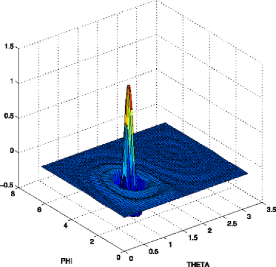
To conclude this section, let us give a graphic representation of a spherical needlet in the spherical coordinates in order to illustrate the above theory. In the following graphic, we chose $j=3$ and $\eta=250$ .

3.3 Besov spaces on the sphere

The problem of choosing appropriated spaces of regularity on the sphere in a serious question, and we decided to consider the spaces which may be the closest to our natural intuition: those which generalize to the sphere case the classical approximation properties used to define for instance Sobolev spaces. In this section, we summarize the main properties of Besov spaces which will be used in the sequel, as established in NarcoPetruWard .

Let $f\dvtx\mathbb{S}^{2}\to\mathbb{R}$ be a measurable function. We define

E_{k}(f,\pi)=\inf_{P\in\mathscr{P}_{k}}\|f-P\|_{\pi},

the $\mathbb{L}_{\pi}$ distance between $f$ and the space $\mathscr{P}_{k}$ of spherical harmonics of degree less than $k$ . The Besov space $B^{s}_{\pi,r}$ is defined as the space of functions such that

f\in\mathbb{L}_{\pi}\quad\mbox{and}\quad\Biggl{(}\sum_{k=0}^{\infty}(k^{s}E_{k}(f,\pi))^{r}\frac{1}{k}\Biggr{)}^{1/r}<+\infty.

Remarking that $k\to E_{k}(f,\pi)$ is decreasing, by a standard condensation argument this is equivalent to

f\in\mathbb{L}_{\pi}\quad\mbox{and}\quad\Biggl{(}\sum_{j=0}^{\infty}(2^{js}E_{2^{j}}(f,\pi))^{r}\Biggr{)}^{1/r}<+\infty,

and the following theorem states that as it is the case for Besov spaces in $\mathbb{R}^{d}$ , the needlet coefficients are good indicators of the regularity and in fact Besov spaces of $\mathbb{S}^{2}$ are Besov bodies, when expressed using needlet expansion. We provide in Figure 1 a graphical representation of a needlet which shows its localization around the associated cubature point.

Theorem 1

Let $1\leq\pi\leq+\infty$ , $s>0$ , $0\leq r\leq+\infty$ . Let $f$ be a measurable function and define

\langle f,\psi_{j,\eta}\rangle=\int_{\mathbb{S}^{2}}f(x)\psi_{j,\eta}(x)\,dx\stackrel{{\scriptstyle\mathit{def}.}}{{=}}\beta_{j,\eta},

provided the integrals exist. Then $f$ belongs to $B^{s}_{\pi,r}$ if and only if, for every $j=1,2,\ldots,$

\biggl{(}\sum_{\eta\in\mathscr{X}_{j}}(|\beta_{j,\eta}|\|\psi_{j,\eta}\|_{\pi})^{\pi}\biggr{)}^{1/\pi}=2^{-js}\delta_{j},

where $(\delta_{j})_{j}\in\ell_{r}$ .

Refer to caption — Figure 1: A spherical needlet.

As has been shown above,

c2^{2j(1/2-1/\pi)}\leq\|\psi_{j,\eta}\|_{\pi}\leq C2^{2j(1/2-1/\pi)}

for some positive constants $c,C$ , the Besov space $B^{s}_{\pi,r}$ turns out to be a Banach space associated to the norm

\|f\|_{B^{s}_{\pi,r}}:=\bigl{\|}\bigl{(}2^{j[s+2(1/2-1/\pi)]}\|(\beta_{j\eta})_{\eta\in\mathscr{Z}_{j}}\|_{\ell_{\pi}}\bigr{)}_{j\geq 0}\bigr{\|}_{\ell_{r}}<\infty,

(30)

and using standard arguments (reducing to comparisons of $l_{q}$ norms), it is easy to prove the following embeddings:

	$\displaystyle B^{s}_{\pi,r}$	$\displaystyle\subset$	$\displaystyle B^{s}_{p,r}\qquad\mbox{for }p\leq\pi,$
	$\displaystyle B^{s}_{\pi,r}$	$\displaystyle\subset$	$\displaystyle B^{s-2(1/\pi-1/p)}_{p,r}\qquad\mbox{for }\pi\leq p\mbox{ and }s>2\biggl{(}\frac{1}{\pi}-\frac{1}{p}\biggr{)}.$

Moreover, it is also true that for $s>\frac{2}{\pi}$ , if $f$ belongs to $B^{s}_{\pi,r}$ , then it is continuous, and as a consequence bounded.

In the sequel, we shall denote by $B^{s}_{\pi,r}(M)$ the ball of radius $M$ of the Besov space $B^{s}_{\pi,r}$ .

4 Needlet algorithm: Thresholding the needlet coefficients

The first step is to construct a needlet system (frame) $\{\psi_{j\eta}\dvtx\eta\in\mathscr{Z}_{j},j\geq-1\}$ as described in Section 3.

The needlet decomposition of any $f\in\mathbb{L}_{2}(\mathbb{S}^{2})$ takes the form

f=\sum_{j}\sum_{\eta\in\mathscr{Z}_{j}}(f,\psi_{j\eta})_{\mathbb{L}_{2}(\mathbb{S}^{2})}\psi_{j\eta}.

Using Parseval’s identity, we have $\beta_{j\eta}=(f,\psi_{j\eta})_{\mathbb{L}_{2}(\mathbb{S}^{2})}=\sum_{lm}\hat{f}^{l}_{m}\psi_{j\eta}^{lm}$ with $\hat{f}^{l}_{m}=(f,Y^{l}_{m})$ and $\psi_{j\eta}^{lm}=(\psi_{j\eta},Y^{l}_{m})$ .

Thus,

\hat{\beta}_{j\eta}=\sum_{lm}\hat{f}^{l,N}_{m}\psi_{j\eta}^{lm},

(32)

is an unbiased estimate of $\beta_{j\eta}$ . We recall that $\hat{f}^{l,N}_{m}$ has been defined in (2.1). It is worthwhile pointing out that the SVD-estimate of the Fourier coefficient $\hat{f}^{l,N}_{m}$ appears in the expression of the estimate $\hat{\beta}_{j\eta}$ . This underlines that the Needlet dictionary does not depart too much from the Fourier basis and hence benefits from the inversion property while being very well localized.

Notice that from the needlet construction (see the previous section) it follows that the sum above is finite. More precisely, $\psi_{j\eta}^{lm}\not=0$ only for $2^{j-1}<l<2^{j+1}$ .

Let us consider the following estimate of $f$ :

\hat{f}=\sum_{j=-1}^{{J}}\sum_{\eta\in\mathscr{Z}_{j}}t(\hat{\beta}_{j\eta})\psi_{j\eta},

(33)

where $t$ is a thresholding operator defined by

$\displaystyle t(\hat{\beta}_{j\eta})$	$\displaystyle=$	$\displaystyle\hat{\beta}_{j\eta}I\{\|\hat{\beta}_{j\eta}\|\geq{\kappa}t_{N}{\|\sigma_{j}\|}\}\qquad\mbox{with}$	(34)
$\displaystyle t_{N}$	$\displaystyle=$	$\displaystyle\sqrt{\frac{\log N}{N}},$	(35)
$\displaystyle\sigma_{j}^{2}$	$\displaystyle=$	$\displaystyle A\sum_{ln}\biggl{\|}\sum_{m}\psi_{j\eta}^{lm}\hat{f}^{l}_{\varepsilon^{-1}mn}\biggr{\|}^{2}.$	(36)

Here $\kappa$ is a tuning parameter of the method which will be properly selected later on. $A$ is chosen such that $\|f_{Z}\|_{\infty}\leq A$ . The choice of these parameters will be discussed later. Notice that the thresholding depends on the resolution level $j$ through the constant $\sigma_{j}$ . As usual in inverse problems, the upper level of details $J$ will be chosen depending of the degree of ill-posedness. It is precisely defined in Theorem 2.

4.1 Performances of the procedure

The following theorem considers the case of a $\mathbb{L}_{p}$ loss with $1\leq p<\infty$ . The case $p=\infty$ is studied in Theorem 3.

Theorem 2

Let $1\leq p<\infty$ , $\nu>0$ , and let us assume that

\sigma_{j}^{2}:=A\sum_{ln}\biggl{|}\sum_{m}\psi_{j\eta}^{lm}\hat{f}^{l}_{\varepsilon^{-1}mn}\biggr{|}^{2}\leq C2^{2j\nu}\qquad\forall j\geq 0.

(37)

$A$ is chosen such that $\|f_{Z}\|_{\infty}\leq A$ . Let us choose $\kappa$ such that $\kappa\geq\sqrt{3\pi}A$ and $\sqrt{3\pi}A\kappa>\max\{8p,2p+1\}$ . Let us also take $2^{J}=\tau[t_{N}]^{-1/(\nu+1)}$ with $t_{N}$ as in $(\ref{tn})$ and $\tau$ is a positive constant. Then if $\pi\geq 1,$ $s>2/\pi$ , $r\geq 1$ $($ with the restriction $r\leq\pi$ if $s=(\nu+1)(\frac{p}{\pi}-1))$ , there exists a constant $T$ such that

\sup_{f\in B^{s}_{\pi,r}(M)}\mathbb{E}\|\hat{f}-f\|_{p}^{p}\leq T(\log(N))^{p-1}\bigl{[}N^{-1/2}\sqrt{\log(N)}\bigr{]}^{\mu p},

(38)

where

	$\displaystyle\mu$	$\displaystyle=$	$\displaystyle\frac{s}{s+\nu+1},\qquad\mbox{if }s\geq(\nu+1)\biggl{(}\frac{p}{\pi}-1\biggr{)},$
	$\displaystyle mu$	$\displaystyle=$	$\displaystyle\frac{s-2/\pi+2/p}{s+\nu-2/\pi+1},\qquad\mbox{if }\frac{2}{\pi}<s<(\nu+1)\biggl{(}\frac{p}{\pi}-1\biggr{)}.$

The following theorem considers the case of $L_{\infty}$ norm loss.

Theorem 3

For $\nu>0$ , let us assume that there exist two constants $C$ , $C^{\prime}$ such that

C^{\prime}2^{2j\nu}\leq\sigma_{j}^{2}:=A\sum_{ln}\biggl{|}\sum_{m}\psi_{j\eta}^{lm}\hat{f}^{l}_{\varepsilon^{-1}mn}\biggr{|}^{2}\leq C2^{2j\nu}\qquad\forall j\geq 0.

(39)

$A$ is chosen such that $\|f_{Z}\|_{\infty}\leq A$ . Let us choose $\kappa$ such that $\kappa\geq\sqrt{3\pi}A$ and $\sqrt{3\pi}A\kappa>16$ . Let us also take $2^{J}=\tau[t_{N}]^{-1/(\nu+1)}$ with $t_{N}$ as in $(\ref{tn})$ and $\tau$ is a positive constant. Then if $\pi\geq 1,$ $s>2/\pi$ , $r\geq 1$ , there exists a constant $T$ such that

\sup_{f\in B^{s}_{\pi,r}(M)}\mathbb{E}\|\hat{f}-f\|_{\infty}\leq T\log(N)[t_{N}]^{\mu^{\prime}},

(40)

where

\mu^{\prime}=\frac{s-2/\pi}{s+\nu-2/\pi+1}.

The proof of these theorems is given in Section 6.

{rem*}

1.

In Theorem 2, the rates of convergence obtained for larger $s$ are usually referred to as the dense case, whereas the other case is referred to as the sparse case.
2.

The parameter $\nu$ appearing here is often called degree of ill-posedness of the problem (DIP). It appears here through conditions (37) and (39) which are essential in this problem. In Kimoptimalspherical , for instance, and very often in diverse inverse problems, this DIP parameter is introduced with the help of the eigenvalues of the operator (i.e., here the discrepancy of the coefficients of $f_{\varepsilon}$ in its expansion along the rotational harmonics). In the following subsection, we prove that (37) and (39) are in fact a consequence of (and even equivalent to) the standard “ordinary smooth” condition.
3.

The rates of convergence found here are standard in inverse problems. They can be related to rates found in Kim and Koo Kimoptimalspherical in the same deconvolution problem, with a $\mathbb{L}_{2}$ loss and constraints on the spaces comparable to $B^{s}_{22}(M)$ . In the deconvolution problem on the interval, similar rates are found even for $\mathbb{L}_{p}$ losses (with standard modifications since the dimension here is 2 instead of 1): see, for instance, Johnstone et al. jkpr . These results are proved to be minimax (see Kim and Koo Kimoptimalspherical ) up to logarithmic factors, for the case $p=2$ with a $B^{s}_{22}(M)$ constraint on the object to estimate. With methods comparatively similar to those in Willer Thomas , it could be proved that our rates are also minimax in the general case (again up to logarithmic factors) if we assume condition (39) (or, in other terms, that the DIP is exactly of the order $\nu$ ).
4.

It is interesting to notice that Theorem 3 proves that the same algorithm is also working for the $\mathbb{L}_{\infty}$ norm, with a slightly more sophisticated proof. It is often the most useful loss function in practice. The proof requires (39) instead of (37). We do not know if this condition is necessary.
5.

It is worthwhile noticing that the procedure is adaptive, meaning that it does not require a priori knowledge on the regularity (or sparsity) of the function. It also adapts to nonhomogeneous smoothness of the function. The logarithmic factor is a standard price to pay for adaptation.
6.

The procedure requires the knowledge of the constant $A$ which is corresponding to the $\mathbb{L}_{\infty}$ norm of the density $f_{Z}$ . It is obvious (because of the convolution) that $A\leq M$ . However, it should be better to obtain a procedure not depending on $M$ either. For that, we advocate that $\|f_{Z}\|_{\infty}$ can be replaced by $\|\hat{f}_{Z}(j_{N}))\|_{\infty}$ in practice where $\hat{f}_{Z}(j_{N}))$ is an undersmoothed needlet estimator of the density $f_{Z}$ close to those introduced in Baldi et al. BaldiKerkMariPica but with no thresholding and with the level $j_{N}$ chosen so that $2^{2j_{N}}\simeq N/(\log N)^{2}$ . Standard arguments similar as in Giné and Nickl GineNickl10b ) imply that this random quantity exponentially concentrates around $\|f_{Z}\|_{\infty}$ . We can also adopt a more straightforward strategy as detailed in Section 5.

4.2 Conditions (37), (39) and the smoothness of $f_{\varepsilon}$

Following Kim and Koo (Kimoptimalspherical , condition (3.6)), we can define the smoothness of $f_{\varepsilon}$ spectrally. We place ourselves in the “ordinary smooth” case

\|(\hat{f}^{l}_{\varepsilon})^{-1}\|_{\mathrm{op}}\leq d_{0}l^{\nu}\quad\mbox{and}\quad\|\hat{f}^{l}_{\varepsilon}\|_{\mathrm{op}}\leq d_{1}l^{-\nu}\qquad\mbox{as }l\rightarrow\infty

(41)

for some positive constants $d_{0}$ , $d_{1}$ and nonnegative constant $\nu$ , and where the operator norm of the rotational Fourier transform $\hat{f}^{l}_{\varepsilon}$ is defined as

\|\hat{f}^{l}_{\varepsilon}\|_{\mathrm{op}}=\sup_{h\neq 0,h\in\mathbb{H}_{l}}\frac{\|\hat{f}^{l}_{\varepsilon}h\|_{2}}{\|h\|_{2}},

$\mathbb{H}_{l}$ being the $(2l+1)$ -dimensional vector space spanned by $\{Y^{l}_{m}\dvtx-l\leq m\leq l\}$ .

The following proposition states that condition (37) [resp. (39)] is verified in the ordinary smooth case by the needlets system.

Proposition 1

If $\|(\hat{f}^{l}_{\varepsilon})^{-1}\|_{\mathrm{op}}\leq d_{0}l^{\nu}$ , then there exists a constant $C$ such that

|\sigma_{j}|^{2}:=A\sum_{ln}\biggl{|}\sum_{m}\psi_{j\eta}^{lm}\hat{f}^{l}_{\varepsilon^{-1}mn}\biggr{|}^{2}\leq C2^{2j\nu}\qquad\forall j\geq 0.

If $\|\hat{f}^{l}_{\varepsilon}\|_{op}\leq d_{0}l^{-\nu}$ , then there exists a constant $C^{\prime}$ such that

|\sigma_{j}|^{2}:=A\sum_{ln}\biggl{|}\sum_{m}\psi_{j\eta}^{lm}\hat{f}^{l}_{\varepsilon^{-1}mn}\biggr{|}^{2}\geq C^{\prime}2^{2j\nu}\qquad\forall j\geq 0.

The proof of this proposition is given in the supplement article (Kerkyacharian et al. KerkPhamPicardA ).

Notice also that the super smooth case (corresponding to exponential spectral decreasing) is also considered in Kim and Koo Kimoptimalspherical . We will not consider this case here, although this could be done, basically because this case corresponds to very poor rates of convergence (logarithmic in $N$ ). As well, this case does not require a thresholding since the adaptation is obtained almost for free.

We now give a brief review of some examples of smooth distributions which are discussed in depth in Healy, Hendriks and Kim HealyHendriksKim and Kim and Koo Kimoptimalspherical .

4.2.1 Rotational Laplace distribution

This distribution can be viewed as an exact analogy on $\mathit{SO}(3)$ of the Laplace distribution on $\mathbb{R}$ . Spectrally, for some $\rho^{2}>0$ , this distribution is characterized by

\hat{f}^{l}_{\varepsilon,mn}=\bigl{(}1+\rho^{2}l(l+1)\bigr{)}^{-1}\delta_{mn}

(42)

for $-l\leq m,n\leq l$ and $l=0,1,\ldots,$ and where $\delta_{mn}=1$ if $m=n$ and $0$ otherwise.

4.2.2 The Rosenthal distribution

This distribution has its origin in random walks in groups (for details, see Rosenthal Rosenthal ).

If one considers the situation where $f_{\varepsilon}$ is a $p$ -fold convolution product of conjugate invariant random for a fixed axis, then Rosenthal (Rosenthal , page 407) showed that

\hat{f}^{l}_{\varepsilon,mn}=\biggl{(}\frac{\sin(l+1/2)\theta}{(2l+1)\sin\theta/2}\biggr{)}^{p}\delta_{mn}

for $-l\leq m,n\leq l$ and $l=0,1,\ldots,$ and where $0<\theta\leq\pi$ and $p>0$ .

5 Practical performances

In this section, we produce the results of numerical experiments on the sphere $\mathbb{S}^{2}$ . Numerical work has been conducted using the spherical pixelization HEALPix software package. HEALPix provides an approximate quadrature of the sphere with a number of data points of order $C2^{2J}$ and a number of quadrature weights of order $\frac{1}{C2^{2J}}$ , for some positive constant $C$ . This approximation is considered as reliable enough and commonly used in astrophysics.

In the two examples below, we considered samples of cardinality $N=1500$ . The maximal resolution level $J$ is taken such that $J=(1/2)\log_{2}(\frac{N}{\log N})$ . In order not to have more cubature points than observations, we set $J=3$ for $N=1500$ . We recall the expression of the estimate of the needlets coefficients of the density of interest:

\hat{\beta}_{j\eta}=\frac{1}{N}\sqrt{\lambda_{j\eta}}\sum_{l=2^{j-1}}^{2^{j+1}}b(l/2^{j})\sum_{m=-l}^{l}\overline{Y^{l}_{m}(\xi_{j\eta})}\sum_{n=-l}^{l}\hat{f}^{l}_{\varepsilon^{-1},mn}\sum_{u=1}^{N}{Y}^{l}_{n}(Z_{u}),

(43)

where the quadrature weight are approximately uniform, $\lambda_{j\eta}\simeq 4\pi/(12.2^{2j})$ . We replace the rotational Fourier transform $(\hat{f}^{l}_{\varepsilon})_{mn}:=\hat{f}^{l}_{\varepsilon,mn}$ [defined in (6)] by its empirical version, more tractable in our simulation study. Note also that this situation is very likely to occur for instance in the context of astrophysics.

We precise again that $\hat{f}^{l}_{\varepsilon^{-1},mn}$ denotes the $(m,n)$ element of the matrix $(\hat{f}^{l}_{\varepsilon})^{-1}:=\hat{f}^{l}_{\varepsilon^{-1}}$ which is the inverse of the $(2l+1)\times(2l+1)$ matrix $(\hat{f}^{l}_{\varepsilon})$ . In order to get the empirical version $\hat{f}^{l,N}_{\varepsilon^{-1},mn}$ of $\hat{f}^{l}_{\varepsilon^{-1},mn}$ , we have first to compute the empirical matrix $(\hat{f}^{l,N}_{\varepsilon})$ then to inverse it to get the matrix $(\hat{f}^{l,N}_{\varepsilon})^{-1}:=\hat{f}^{l,N}_{\varepsilon^{-1}}$ . The $(m,n)$ entry of the matrix $(\hat{f}^{l,N}_{\varepsilon})$ is given by the formula

\hat{f}^{l,N}_{\varepsilon,mn}=\frac{1}{N}\sum_{j=1}^{N}D^{l}_{m,n}(\varepsilon_{j}),

where the rotational harmonics $D^{l}_{m,n}$ have been defined in (4). The $\varepsilon_{j}$ ’s are i.i.d. realizations of the variable $\varepsilon\in\mathit{SO}(3)$ .

For the generation of the random variable $\varepsilon\in\mathit{SO}(3)$ , we chose Oz as the rotation axis and an angle $\phi$ following a uniform law with different supports such as $[0,\pi/8]$ , $[0,\pi/4]$ , $[0,\pi/2]$ . The larger the support of distribution is, the more intense the effect of the noise will be.

This particular choice of rotation matrix entails that in the decomposition of an element of $\mathit{SO}(3)$ [see formula (3)] the angles $\psi$ and $\theta$ are both equal to zero. For this specific setting of perturbation, we deduce the following form for the rotational harmonics:

D^{l}_{m,n}(\varepsilon_{j})=P^{l}_{mn}(1)e^{-ni\phi_{j}}=\delta_{mn}e^{-in\phi_{j}},

where $\phi_{j}\sim U[0,a]$ and $a$ is a positive constant which will be specified later.

Choosing $\sigma_{j}$ . As one may notice, the estimator $\hat{f}$ [see (33)] relies on the knowledge of $A$ which controls the sup norm of the density $f_{Z}$ and appears in the formula of $\sigma^{2}_{j}$ , see (36). Different ways to circumvent this difficulty can be used, for instance, estimating it as explained above. However, we have adopted in this section a different approach. The quantity $\sigma_{j}^{2}$ constitutes a control of the variance of the estimated coefficients $\hat{\beta}_{j\eta}$ as it is shown by inequality (5) in the supplementary material (see Kerkyacharian et al. KerkPhamPicardA ). Using this remark, instead of using an upper bound of the variance of $\hat{\beta}_{j\eta}$ , we will directly plug in an estimation of this variance. Hence, $\sigma_{j}^{2}$ in (34) is replaced by

v_{j\eta}^{2}=\frac{1}{(N-1)}\sum_{i=1}^{N}|G_{j\eta}(Z_{i})-\widetilde{G_{j\eta}}(Z)|^{2},

where

G_{j\eta}(x)=\sum_{lm}\psi^{lm}_{j\eta}\sum_{n}\hat{f}^{l}_{\varepsilon^{-1},mn}Y^{l}_{n}(x)

and

\widetilde{G_{j\eta}}(Z)=\frac{1}{N}\sum_{i=1}^{N}G_{j\eta}(Z_{i}).

Remark that $\hat{\beta}_{j\eta}=\frac{1}{N}\sum_{i=1}^{N}G_{j\eta}(Z_{i})$ .

Hence, for the reconstruction of the density $f$ , we have the following Needlet estimator:

\hat{f}:=\frac{1}{|\mathbb{S}^{2}|}+\sum_{j=0}^{J}\sum_{\eta=1}^{12.2^{2j}}\hat{\beta}_{j\eta}\psi_{j\eta}I_{\{|\hat{\beta}_{j\eta}|\geq\kappa t_{N}|v_{j\eta}|\}}.

Choosing the tuning parameter $\kappa$ . Before entering into the details of the numerical results, we will dwell on the methodology used in this part to calibrate the tuning paramater $\kappa$ in practice. In a first time, we focus on the uniform density. Indeed, we make an upstream study with the uniform density $f=\frac{1}{4\pi}\mathbf{1}_{\mathbb{S}^{2}}$ which will allow us to determine a reasonable value for $\kappa$ which will be kept in the sequel for other types of densities. On the one hand, the choice of the uniform density is not fortuitous because we know that in theory the needlet coefficient $\langle f,\psi_{j\eta}\rangle=0$ for all $j$ and $\eta$ . On the other hand, for an upstream study, a prerequisite is to deal with a simple density, which is the case. Hence, we test various values of $\kappa$ and see how many coefficients survive thresholding. Then we look at the smallest value of $\kappa$ for which all the estimated coefficients are killed. It turns out that $\kappa=0.5$ . Consequently for $\kappa=0.5,$ we have noise-free reconstructions of the uniform density. Accordingly, this particular value of $\kappa$ plays a benchmark value for the other types of density that we highlight. In other words, in the Example 2, which concerns the unimodal density we set $\kappa=0.5$ .

We can form a parallel to what happens on the real line. Indeed, in a certain way, this strategy for choosing $\kappa$ in practise meets up with the universal threshold $\sqrt{2\log n}$ put forward by Donoho and Johnstone DonohoJohnstone in the context of fixed design regression on $\mathbb{R}$ in order to “kill” asymptotically all the coefficients when estimating the zero function. Then, we compute the $\mathbb{L}_{2}$ and $\mathbb{L}_{\infty}$ losses and give the graphic reconstructions. This choice of $\kappa$ turns out to be very reasonable and fruitful as the results prove to be good enough.

\tablewidth

=265pt $\bolds{j=0}$ $\bolds{j=1}$ $\bolds{j=2}$ $\bolds{j=3}$ $\kappa=0.2$ 0 7 30 110 $\kappa=0.3$ 0 0 2 6 $\kappa=0.4$ 0 0 0 3

Table 1: Number of coefficients surviving thresholdingfor various values of

\kappa

\phi\sim U[0,\pi/8]

\tablewidth

=265pt $\bolds{j=0}$ $\bolds{j=1}$ $\bolds{j=2}$ $\bolds{j=3}$ $\kappa=0.2$ 2 3 77 350 $\kappa=0.3$ 0 0 4 10 $\kappa=0.4$ 0 0 0 6

Table 2: Number of coefficients surviving thresholding for various values of

\kappa

\phi\sim U[0,\pi]

Example 1.

In this first example, we consider the case of the uniform density $f=\frac{1}{4\pi}\mathbf{1}_{\mathbb{S}^{2}}$ . It is easy to verify that $\beta_{j\eta}=\langle f,\psi_{j\eta}\rangle_{\mathbb{L}_{2}}=0$ for every $j$ and every $\eta$ . Following Baldi et al. BaldiKerkMariPica , a simple way of assessing the performance of the Needlet procedure is to count the number of coefficients surviving thresholding.

We precise that both in the cases of an angle following a law $U[0,\pi/8]$ or $U[0,\pi]$ , all the coefficients are killed for $\kappa=0.5$ (see Tables 1 and 2). Accordingly, we can conclude that the thresholding procedure based on spherical needlets is very efficient.

Example 2.

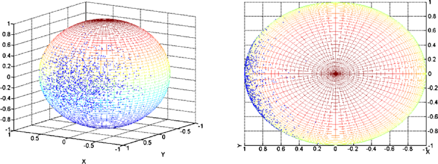
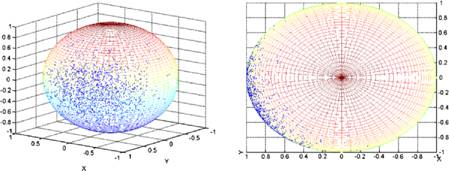
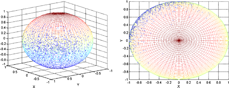
We will now deal with the example of a density of the form $f(\omega)=ce^{-4|\omega-\omega_{1}|^{2}}$ , with $\omega_{1}=(0,1,0)$ and $c=1/0.7854$ . The graph of $f$ in the spherical coordinates $(\Phi,\Theta)$ ( $\Phi={}$ longitude, $0\leq\Phi\leq 2\pi$ , $\Theta={}$ colatitude, $0\leq\Theta\leq\pi$ ) is given in Figure 2. We also plot the noisy observations for different cases of perturbations. For big rotation angles such that $\phi\sim U[0,\pi/4]$ or $\phi\sim U[0,\pi/2]$ , the observations tend to be spread over a large region on the sphere and not to be concentrated in a specific region any more. Consequently, denoising might prove to be difficult. In the context of the deconvolution on the sphere, a large amount of noise corresponds to a rotation about the Oz axis by a large angle.

As motivated above, in the sequel, the tuning parameter $\kappa$ for the Needlet procedure is set to $0.5$ both for computing the quadratic loss, the $L_{\infty}$ loss and the graphic reconstructions.

\tablewidth

=265pt $\bolds{\phi\sim U[0,\pi/8]}$ $\bolds{\phi\sim U[0,\pi/4]}$ $\bolds{\phi\sim U[0,\pi/2]}$ $\mathbb{L}_{2}$ 0.3335 0.5523 0.7830 $\mathbb{L}_{\infty}$ 0.1019 0.1677 0.1928

Table 3:

\mathbb{L}_{2}

and

\mathbb{L}_{\infty}

estimated losses

First of all, we have computed an estimate of the $\mathbb{L}_{2}$ and the $\mathbb{L}_{\infty}$ norms of the difference between $\hat{f}$ our Needlet estimator and $f$ (see Table 3). For the quadratic loss, we took the square root of the sum of the squares of the coefficients. As for the $\mathbb{L}_{\infty}$ distance, we chose an almost uniform grid of the sphere $\mathbb{S}^{2}$ given by the HEALPix pixelization program. We recall that

\|\hat{f}-f\|_{\infty}=\sup_{i=1,\ldots,L}|\hat{f}(\alpha_{i})-f(\alpha_{i})|,

where the $\alpha_{i}$ are the points of a uniform grid of the sphere. Here, we chose $L=192=12.2^{4}$ . All the estimated losses were computed over $50$ runs and for $N=1500$ observations. We considered the three cases of noise level described above. The results are summarized in the following table of errors which shows that the estimator performs quite well. In particular, its performances are deteriorating when the noise becomes more important (which was expected) and give very good results in $\mathbb{L}_{\infty}$ norm. We concentrated on particular phenomena instead of performing a large scanning of the errors in very diverse situations because the computations—although feasible—are rather costly in time when used repeatedly. For instance, to our knowledge, and probably for the same reason, no such study has been performed for the SVD method.

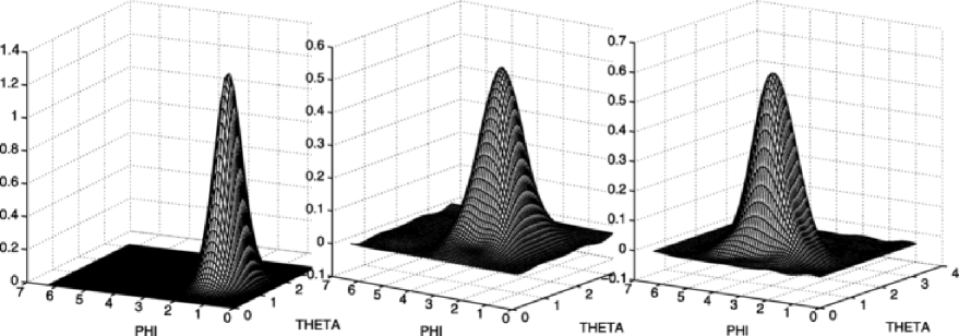
SVD versus needlet on a particular problem. A central issue in Astrophysics is to detect the place of the peak of the bell which in the present density case is localized in $(\Theta=\pi/2,\Phi=\pi/2)$ . For each case of noise, we plot the observations both on the sphere and on the flattened sphere and give the reconstructed density in the spherical coordinates for the Needlet procedure and the SVD estimator (see Figures 2, 4 and 6).

For each of the three groups of graphic reconstructions of the target density presented below corresponding to three cases of noise, you will find in order, the exact target density, then the one estimated with the Needlet procedure and finally the density estimated with the SVD method (see Figures 3, 5 and 7).

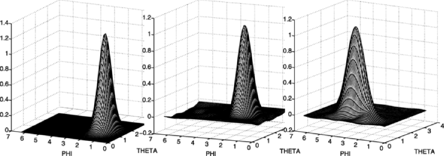
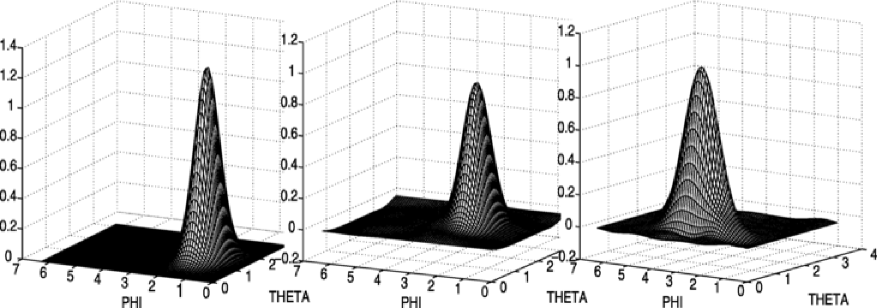
At a closer inspection, we notice that the position of the peak of the estimated bell is well localized by the Needlet procedure whatever the amount of noise, it is especially true for $\phi\sim U[0,\pi/8]$ . Only in the case of the law $U[0,\pi/2]$ , the longitude coordinate of the peak tends to slightly move away from the true value. As for the SVD method, for the three reconstructions, it fails to detect properly the exact position of the peak. Therefore, even if in the case of big rotations such that $\phi\sim U[0,\pi/4]$ and especially $\phi\sim U[0,\pi/2]$ , the Needlet procedure allows us to have a rather good detection of the position of the peak. This is of course due to the remarkable concentration of the needlet. Of course, one remarks that the base of the bell tends to become a bit larger when the noise increases, this is due to the fact that the observations are not concentrated in a specific region any longer, but the genuine form of the density is well preserved.

6 Proof of Theorems 2 and 3

In this proof, $C$ will denote an absolute constant which may change from one line to the other.

We begin with the following proposition.

Proposition 2

For any $q\geq 1$ there exist constants $C,s_{q},s^{\prime}_{q}$ , such that, as soon as $2^{j}\leq[\frac{N}{\log N}]^{1/2}$ ,

$\displaystyle\hskip 45.0pt\mathbb{P}\{\|\hat{\beta}_{j\eta}-\beta_{j\eta}\|\geq\sigma_{j}v\}$	$\displaystyle\leq$	$\displaystyle 2\exp\biggl{\{}-\frac{Nv^{2}}{2(1+2/(\sqrt{3\pi}A)v2^{j})}\biggr{\}}\qquad\forall v>0,$	(44)
$\displaystyle\mathbb{E}\|\hat{\beta}_{j\eta}-\beta_{j\eta}\|^{q}$	$\displaystyle\leq$	$\displaystyle s_{q}\biggl{[}\frac{\sigma_{j}^{2}}{N}\biggr{]}^{q/2},$	(45)
$\displaystyle\mathbb{E}\sup_{\eta}\|\hat{\beta}_{j\eta}-\beta_{j\eta}\|^{q}$	$\displaystyle\leq$	$\displaystyle s_{q}^{\prime}(j+1)^{q}\biggl{[}\frac{\sigma_{j}^{2}}{N}\biggr{]}^{q/2},$	(46)
$\displaystyle\mathbb{P}(\|\hat{\beta}_{j\eta}-\beta_{j\eta}\|\geq\sigma_{j}{\kappa}t_{N})$	$\displaystyle\leq$	$\displaystyle 2N^{-\sqrt{3\pi}A\kappa/4}\qquad\forall\kappa\geq\sqrt{3\pi}A.$	(47)

The proof of this proposition is given in the supplementary material (see Kerkyacharian et al. KerkPhamPicardA ).

6.1 Proof of Theorem 2

Now, to get the result of Theorem 2, we begin by the following decomposition:

	$\displaystyle\hskip 2.0pt\mathbb{E}\\|\hat{f}-f\\|_{p}^{p}$	$\displaystyle\leq$	$\displaystyle 2^{p-1}\Biggl{\{}\mathbb{E}\Biggl{\\|}\sum_{j=-1}^{{J}}\sum_{\eta\in\mathscr{Z}_{j}}\bigl{(}t(\hat{\beta}_{j\eta})-\beta_{j\eta}\bigr{)}\psi_{j\eta}\Biggr{\\|}_{p}^{p}+\biggl{\\|}\sum_{j>{J}}\sum_{\eta\in\mathscr{Z}_{j}}\beta_{j\eta}\psi_{j\eta}\biggr{\\|}_{p}^{p}\Biggr{\}}$
		$\displaystyle=:$	$\displaystyle I+\mathit{II}.$

The term $\mathit{II}$ is easy to analyze, as follows. We observe first that since $B^{s}_{\pi,r}(M)\subset B^{s}_{p,r}(M^{\prime})$ for $\pi\geq p$ , this case will be assimilated to the case $\pi=p$ and from now on, we will only consider $\pi\leq p$ . Since $f$ belongs to $B^{s}_{\pi,r}(M)$ , using the embedding results recalled above in (3.3), we have that $f$ also belongs to $B^{s-(2/\pi-2/p)}_{p,r}(M^{\prime})$ , for some constant $M^{\prime}$ and for $\pi\leq p$ . Hence,

\biggl{\|}\sum_{j>{J}}\sum_{\eta\in\mathscr{Z}_{j}}\beta_{j\eta}\psi_{j\eta}\biggr{\|}_{p}\leq C2^{-J[s-2(1/\pi-1/p)]}.

Then we only need to verify that $\frac{s-2(1/\pi-1/p)}{\nu+1}$ is always larger that $\mu$ , which is not difficult.

Indeed, on the first zone $s\geq(\nu+1)(p/\pi-1)$ . So, $s+\nu+1\geq(\nu+1)\frac{p}{\pi}$ which entails that $\frac{s}{(s+\nu+1)}\leq\frac{s}{(\nu+1)p/\pi}$ . We need to check that $s-2(\frac{1}{\pi}-\frac{1}{p})\geq\frac{s\pi}{p}$ . We have that $s-\frac{2}{\pi}+\frac{2}{p}-\frac{s\pi}{p}=2(\frac{s\pi}{2}-1)(\frac{1}{\pi}-\frac{1}{p})\geq 0$ since $s\geq\frac{2}{\pi}$ and $p\geq\pi$ .
On the second zone, we obviously have that $\frac{s-2(1/\pi-1/p)}{\nu+1}$ is always larger than $\mu=\frac{s-2/\pi+2/p}{s+\nu-2/\pi+1}$ .

Bounding the term I is more involved. Using the triangular inequality together with Hölder inequality, and property (28) for the second line, we get

	$\displaystyle I$	$\displaystyle\leq$	$\displaystyle 2^{p-1}J^{p-1}\sum_{j=-1}^{{J}}\mathbb{E}\biggl{\\|}\sum_{\eta\in\mathscr{Z}_{j}}\bigl{(}t(\hat{\beta}_{j\eta})-\beta_{j\eta}\bigr{)}\psi_{j\eta}\biggr{\\|}_{p}^{p}$
		$\displaystyle\leq$	$\displaystyle 2^{p-1}J^{p-1}C\sum_{j=-1}^{{J}}\sum_{\eta\in\mathscr{Z}_{j}}\mathbb{E}\|t(\hat{\beta}_{j\eta})-\beta_{j\eta}\|^{p}\\|\psi_{j\eta}\\|_{p}^{p}.$

Now, we separate four cases:

	$\displaystyle\sum_{j=-1}^{{J}}\sum_{\eta\in\mathscr{Z}_{j}}\mathbb{E}\|t(\hat{\beta}_{j\eta})-\beta_{j\eta}\|^{p}\\|\psi_{j\eta}\\|_{p}^{p}$
	$\displaystyle\qquad=\sum_{j=-1}^{{J}}\sum_{\eta\in\mathscr{Z}_{j}}\mathbb{E}\|t(\hat{\beta}_{j\eta})-\beta_{j\eta}\|^{p}\\|\psi_{j\eta}\\|_{p}^{p}\bigl{\{}I\{\|\hat{\beta}_{j\eta}\|\geq{\kappa}t_{N}{\sigma_{j}}\}$
	$\displaystyle\hphantom{\qquad=\sum_{j=-1}^{{J}}\sum_{\eta\in\mathscr{Z}_{j}}\mathbb{E}\|t(\hat{\beta}_{j\eta})-\beta_{j\eta}\|^{p}\\|\psi_{j\eta}\\|_{p}^{p}\bigl{\{}}{}+I\{\|\hat{\beta}_{j\eta}\|<{\kappa}t_{N}{\sigma_{j}}\}\bigr{\}}$
	$\displaystyle\qquad\leq\sum_{j=-1}^{{J}}\sum_{\eta\in\mathscr{Z}_{j}}\biggl{[}\mathbb{E}\|\hat{\beta}_{j\eta}-\beta_{j\eta}\|^{p}\\|\psi_{j\eta}\\|_{p}^{p}I\{\|\hat{\beta}_{j\eta}\|\geq{\kappa}t_{N}{\sigma_{j}}\}$
	$\displaystyle\hphantom{\qquad\leq\sum_{j=-1}^{{J}}\sum_{\eta\in\mathscr{Z}_{j}}\biggl{[}}{}\times\biggl{\{}I\biggl{\{}\|\beta_{j\eta}\|\geq\frac{\kappa}{2}t_{N}{\sigma_{j}}\biggr{\}}+I\biggl{\{}\|\beta_{j\eta}\|<\frac{\kappa}{2}t_{N}{\sigma_{j}}\biggr{\}}\biggr{\}}$
	$\displaystyle\hphantom{\qquad\leq\sum_{j=-1}^{{J}}\sum_{\eta\in\mathscr{Z}_{j}}\biggl{[}}{}+\|\beta_{j\eta}\|^{p}\\|\psi_{j\eta}\\|_{p}^{p}I\{\|\hat{\beta}_{j\eta}\|<{\kappa}t_{N}{\sigma_{j}}\}\bigl{\{}I\{\|\beta_{j\eta}\|\geq 2{\kappa}t_{N}{\sigma_{j}}\}$
	$\displaystyle\hphantom{\hphantom{\qquad\leq\sum_{j=-1}^{{J}}\sum_{\eta\in\mathscr{Z}_{j}}\biggl{[}}{}+\|\beta_{j\eta}\|^{p}\\|\psi_{j\eta}\\|_{p}^{p}I\{\|\hat{\beta}_{j\eta}\|<{\kappa}t_{N}{\sigma_{j}}\}\bigl{\{}}{}+I\{\|\beta_{j\eta}\|<2{\kappa}t_{N}{\sigma_{j}}\}\bigr{\}}\biggr{]}$
	$\displaystyle\qquad=:\mathit{Bb}+\mathit{Bs}+\mathit{Sb}+\mathit{Ss}.$

We have the following upper bounds for the terms $\mathit{Bs}$ and $\mathit{Sb}$ :

	$\displaystyle\mathit{Bs}$	$\displaystyle\leq$	$\displaystyle CN^{-\sqrt{3\pi}A\kappa/16},$
	$\displaystyle\mathit{Sb}$	$\displaystyle\leq$	$\displaystyle CN^{-\sqrt{3\pi}A\kappa/2+p/(\nu+1)}.$

It is easy to check that in any cases if $\sqrt{3\pi}A\kappa>\max\{8p,2p+1\}$ the terms $\mathit{Bs}$ and $\mathit{Sb}$ are smaller than the rates announced in the theorem. For the details of the above upper bounds of the terms $\mathit{Bs}$ and $\mathit{Sb}$ , see the supplementary material (Kerkyacharian et al. KerkPhamPicardA ).

Using Proposition 2, we have

	$\displaystyle\mathit{Bb}$	$\displaystyle\leq$	$\displaystyle C\sum_{j=-1}^{{J}}\sum_{\eta\in\mathscr{Z}_{j}}\sigma_{j}^{p}N^{-p/2}\\|\psi_{j\eta}\\|_{p}^{p}I\biggl{\{}\|\beta_{j\eta}\|\geq\frac{\kappa}{2}t_{N}{\sigma_{j}}\biggr{\}},$
	$\displaystyle\mathit{Ss}$	$\displaystyle\leq$	$\displaystyle\sum_{j=-1}^{{J}}\sum_{\eta\in\mathscr{Z}_{j}}\|\beta_{j\eta}\|^{p}\\|\psi_{j\eta}\\|_{p}^{p}I\{\|\beta_{j\eta}\|<2{\kappa}t_{N}{\sigma_{j}}\}.$

Using again Proposition 2, (25) and condition (37) for any $p\geq z\geq 0$ :

$\displaystyle\mathit{Bb}$	$\displaystyle\leq$	$\displaystyle CN^{-p/2}\sum_{j=-1}^{{J}}\sigma_{j}^{p}2^{j(p-2)}\sum_{\eta\in\mathscr{Z}_{j}}I\biggl{\{}\|\beta_{j\eta}\|\geq\frac{\kappa}{2}t_{N}{\sigma_{j}}\biggr{\}}$
	$\displaystyle\leq$	$\displaystyle CN^{-p/2}\sum_{j=-1}^{{J}}\sigma_{j}^{p}2^{j(p-2)}\sum_{\eta\in\mathscr{Z}_{j}}\|\beta_{j\eta}\|^{z}[t_{N}{\sigma_{j}}]^{-z}$
	$\displaystyle\leq$	$\displaystyle C{t_{N}}^{p-z}\sum_{j=-1}^{{J}}2^{j[\nu(p-z)+p-2]}\sum_{\eta\in\mathscr{Z}_{j}}\|\beta_{j\eta}\|^{z}.$

Also, for any $p\geq z\geq 0$ ,

	$\displaystyle\mathit{Ss}$	$\displaystyle\leq$	$\displaystyle C\sum_{j=-1}^{{J}}2^{j(p-2)}\sum_{\eta\in\mathscr{Z}_{j}}\|\beta_{j\eta}\|^{z}\sigma_{j}^{p-z}[t_{N}]^{p-z}$
		$\displaystyle\leq$	$\displaystyle C[t_{N}]^{p-z}\sum_{j=-1}^{{J}}2^{j(\nu(p-z)+p-2)}\sum_{\eta\in\mathscr{Z}_{j}}\|\beta_{j\eta}\|^{z}.$

So in both cases we have the same bound to investigate. We will write this bound on the following form (forgetting the constant):

	$\displaystyle A+B$	$\displaystyle:=$	$\displaystyle{t_{N}}^{p-z_{1}}\Biggl{[}\sum_{j=-1}^{{j_{0}}}2^{j[\nu(p-z_{1})+p-2]}\sum_{\eta\in\mathscr{Z}_{j}}\|\beta_{j\eta}\|^{z_{1}}\Biggr{]}$
			$\displaystyle{}+{t_{N}}^{p-z_{2}}\Biggl{[}\sum_{j=j_{0}+1}^{{J}}2^{j[\nu(p-z_{2})+p-2]}\sum_{\eta\in\mathscr{Z}_{j}}\|\beta_{j\eta}\|^{z_{2}}\Biggr{]}.$

The constants $z_{i}$ and $j_{0}$ will be chosen depending on the cases, with the only constraint $p\geq z_{i}\geq 0$ .

We recall that we only need to investigate the case $p\geq\pi$ , since when $p\leq\pi$ , $B^{s}_{\pi r}(M)\subset B^{s}_{pr}(M^{\prime})$ .

Let us first consider the case where $s\geq(\nu+1)(\frac{p}{\pi}-1)$ , put

q=\frac{p(\nu+1)}{s+\nu+1},

and observe that on the considered domain, $q\leq\pi$ and $p>q$ . In the sequel, it will be useful to observe that we have $s=(\nu+1)(\frac{p}{q}-1)$ . Now, taking $z_{2}=\pi$ , we get

B\leq{t_{N}}^{p-\pi}\Biggl{[}\sum_{j=j_{0}+1}^{{J}}2^{j[\nu(p-\pi)+p-2]}\sum_{\eta\in\mathscr{Z}_{j}}|\beta_{j\eta}|^{\pi}\Biggr{]}.

Now, as

\frac{p}{q}-\frac{2}{\pi}+\nu\biggl{(}\frac{p}{q}-1\biggr{)}=s+1-\frac{2}{\pi}

and

\sum_{\eta\in\mathscr{Z}_{j}}|\beta_{j\eta}|^{\pi}=2^{-j\pi(s+1-2/\pi)}\tau_{j}^{\pi},

with $(\tau_{j})_{j}\in l_{r}$ (this last thing is a consequence of the fact that $f\in B^{s}_{\pi,r}(M)$ ), we can write

	$\displaystyle B$	$\displaystyle\leq$	$\displaystyle{t_{N}}^{p-\pi}\sum_{j=j_{0}+1}^{J}2^{jp(1-\pi/q)(\nu+1)}\tau_{j}^{\pi}$
		$\displaystyle\leq$	$\displaystyle C{t_{N}}^{p-\pi}2^{j_{0}p(1-\pi/q)(\nu+1)}.$

The last inequality is true for any $r\geq 1$ if $\pi>q$ and for $r\leq\pi$ if $\pi=q$ . Notice that $\pi=q$ is equivalent to $s=(\nu+1)(\frac{p}{\pi}-1).$ Now if we choose $j_{0}$ such that $2^{j_{0}(p/q)(\nu+1)}\sim{t_{N}}^{-1}$ , we get the bound

{t_{N}}^{p-q},

which exactly gives the rate announced in the theorem for this case. As for the first part of the sum (before $j_{0}$ ), we have, taking now $z_{1}=\tilde{q}$ , with $\tilde{q}\leq\pi$ (and also $\tilde{q}\leq p$ since we investigate the case $p\geq\pi$ ), so that $[\frac{1}{2^{2j}}\sum_{\eta\in\mathscr{Z}_{j}}|\beta_{j\eta}|^{\tilde{q}}]^{1/\tilde{q}}\leq[\frac{1}{2^{2j}}\sum_{\eta\in\mathscr{Z}_{j}}|\beta_{j\eta}|^{\pi}]^{1/\pi}$ , we get

$\displaystyle A$	$\displaystyle\leq$	$\displaystyle{t_{N}}^{p-\tilde{q}}\Biggl{[}\sum_{j=-1}^{{j_{0}}}2^{j[\nu(p-\tilde{q})+p-2]}\sum_{\eta\in\mathscr{Z}_{j}}\|\beta_{j\eta}\|^{\tilde{q}}\Biggr{]}$
	$\displaystyle\leq$	$\displaystyle{t_{N}}^{p-\tilde{q}}\Biggl{[}\sum_{j=-1}^{{j_{0}}}2^{j[\nu(p-\tilde{q})+p-2\tilde{q}/\pi]}\biggl{[}\sum_{\eta\in\mathscr{Z}_{j}}\|\beta_{j\eta}\|^{\pi}\biggr{]}^{\tilde{q}/\pi}\Biggr{]}$
	$\displaystyle\leq$	$\displaystyle{t_{N}}^{p-\tilde{q}}\sum_{j=-1}^{{j_{0}}}2^{j[(\nu+1)p(1-\tilde{q}/q)]}\tau_{j}^{\tilde{q}}$
	$\displaystyle\leq$	$\displaystyle C{t_{N}}^{p-\tilde{q}}2^{j_{0}p[(\nu+1)(1-\tilde{q}/q)]}$
	$\displaystyle\leq$	$\displaystyle C{t_{N}}^{p-q}.$

The last two lines are valid if $\tilde{q}$ is chosen strictly smaller than $q$ (this is possible since $\pi\geq q$ ).

Let us now consider the case where $s<(\nu+1)(\frac{p}{\pi}-1)$ , and choose now

q=p\frac{\nu+1-2/p}{s+\nu-2/\pi+1}.

In such a way that we easily verify that $p-q=p\frac{s-2/\pi+2/p}{1+\nu+s-2/\pi},q-\pi=\break\frac{(p-\pi)(1+\nu)-\pi s}{s+\nu-2/\pi+1}>0$ . Furthermore, we also have $s+1-\frac{2}{\pi}=\frac{p}{q}-\frac{2}{q}+\nu(\frac{p}{q}-1)$ . Hence, taking $z_{1}=\pi$ and using again the fact that $f$ belongs to $B^{s}_{\pi,r}(M)$ ,

$\displaystyle A$	$\displaystyle\leq$	$\displaystyle{t_{N}}^{p-\pi}\Biggl{[}\sum_{-1}^{{j_{0}}}2^{j[\nu(p-\pi)+p-2]}\sum_{\eta\in\mathscr{Z}_{j}}\|\beta_{j\eta}\|^{\pi}\Biggr{]}$
	$\displaystyle\leq$	$\displaystyle{t_{N}}^{p-\pi}\sum_{-1}^{{j_{0}}}2^{j[(\nu+1-2/p)(p/q)(q-\pi)]}\tau_{j}^{\pi}$
	$\displaystyle\leq$	$\displaystyle C{t_{N}}^{p-\pi}2^{j_{0}[(\nu+1-2/p)(p/q)(q-\pi)]}.$

This is true since $\nu+1-\frac{2}{p}$ is also strictly positive since $\nu+1>\frac{s}{p/\pi-1}\geq\frac{2}{p-\pi}\geq\frac{2}{p}$ . If we now take $2^{j_{0}(p/q)(\nu+1-2/p)}\sim{t_{N}}^{-1}$ , we get the bound

{t_{N}}^{p-q},

which is the rate announced in the theorem for this case.

Again, for $B$ , we have, taking now $z_{2}=\tilde{q}>q(>\pi)$

B\leq{t_{N}}^{p-\tilde{q}}\Biggl{[}\sum_{j=j_{0}+1}^{{J}}2^{j[\nu(p-\tilde{q})+p-2]}\sum_{\eta\in\mathscr{Z}_{j}}|\beta_{j\eta}|^{\tilde{q}}\Biggr{]}.

But

\sum_{\eta\in\mathscr{Z}_{j}}|\beta_{j\eta}|^{\tilde{q}}\leq C2^{-j\tilde{q}(s+1-2/\pi)}\tau^{\tilde{q}}_{j},

and $s+1-\frac{2}{\pi}=\frac{p}{q}-\frac{2}{q}+\nu(\frac{p}{q}-1)$ , hence

$\displaystyle B$	$\displaystyle\leq$	$\displaystyle C{t_{N}}^{p-\tilde{q}}\sum_{j=j_{0}+1}2^{j[(\nu+1-2/p)(p/q)(q-\tilde{q})]}\tau_{j}^{{\tilde{q}}}$
	$\displaystyle\leq$	$\displaystyle C{t_{N}}^{p-\tilde{q}}2^{j_{0}[(\nu+1-2/p)(p/q)(q-\tilde{q})]}$
	$\displaystyle\leq$	$\displaystyle C{t_{N}}^{p-q},$

which completes the proof of Theorem 2.

6.2 Proof of Theorem 3

The proof of this theorem is entirely given in the supplementary material (see Kerkyacharian et al. KerkPhamPicardA ).

{supplement}

[id=suppA] \stitleSupplement to “Localized spherical deconvolution”
\slink[doi]10.1214/10-AOS858SUPP \sdatatype.pdf \sfilenamesupplementA_Annals.pdf \sdescriptionWe give in the supplement some technical details for the understanding of the proofs of Propositions 1 and 2 and of Theorems 2 and 3.

Acknowledgments

The authors would like to thank Erwan Le Pennec for many helpful discussions and suggestions concerning the simulations. We would also like to thank an Associate Editor and two anonymous referees for their insightful comments on a first draft of this work.

References

(1) Baldi, P., Kerkyacharian, G., Marinucci, D. and Picard, D. (2009). Adaptive density estimation for directional data using needlets. Ann. Statist. 37 3362–3395. \MR2549563
(2) Baldi, P., Kerkyacharian, G., Marinucci, D. and Picard, D. (2009). Subsampling needlet coefficients on the sphere. Bernoulli 15 438–463. \MR2543869
(3) Donoho, D. L and Johnstone, I. M. (1994). Ideal spatial adaptation by wavelet shrinkage. Biometrika 81 425–455. \MR1311089
(4) Giné, E. and Nickl, R. (2010). Adaptive estimation of a distribution function and its density in sup-norm loss by wavelet and spline projections. Bernoulli. To appear.
(5) Healy Jr., D. M., Hendriks, H. and Kim, P. T. (1998). Spherical deconvolution. J. Multivariate Anal. 67 1–22. \MR1659108
(6) Johnstone, I., Kerkyacharian, G., Picard, D. and Raimondo, M. (2004). Wavelet deconvolution in a periodic setting. J. R. Stat. Soc. Ser. B Stat. Methodol. 66 547–573. \MR2088290
(7) Kerkyacharian, G., Kyriazis, G., Le Pennec, E., Petrushev, P. and Picard, D. (2010). Inversion of noisy Radon transform by SVD based needlets. Appl. Comput. Harmonic Anal. 28 24–45. \MR2563258
(8) Kerkyacharian, G. and Picard, D. (2009). New generation wavelets associated with statistical problems. In The 8th Workshop on Stochastic Numerics 119–146. Research Institute for Mathematical Sciences, Kyoto Univ.
(9) Kerkyacharian, G., Pham Ngoc, T. M and Picard, D. (2010). Supplement to “Localized spherical deconvolution.” DOI:10.1214/10-AOS858SUPP.
(10) Kerkyacharian, G., Petrushev, P., Picard, D. and Willer, T. (2007). Needlet algorithms for estimation in inverse problems. Electron. J. Statist. 1 30–76 (electronic). \MR2312145
(11) Kim, P. T. and Koo, J. Y. (2002). Optimal spherical deconvolution. J. Multivariate Anal. 80 21–42. \MR1889831
(12) Narcowich, F., Petrushev, P. and Ward, J. (2006). Decomposition of Besov and Triebel–Lizorkin spaces on the sphere. J. Funct. Anal. 238 530–564. \MR2253732
(13) Narcowich, F., Petrushev, P. and Ward, J. (2006). Local tight frames on spheres. SIAM J. Math. Anal. 38 574–594. \MR2237162
(14) Pietrobon, D., Baldi, P., Kerkyacharian, G., Marinucci, D. and Picard, D. (2008). Spherical needlets for CMB data analysis. Monthly Notices of the Roy. Astron. Soc. 383 539–545.
(15) Rosenthal, J. S. (1994). Random rotations: Characters and random walks on $\mathrm{\mathit{SO}}(N)$ . Ann. Probab. 22 398–423. \MR1258882
(16) Talman, J. D. (1968). Special Functions: A Group Theoretic Approach. W. A. Benjamin, New York. \MR0239154
(17) Terras, A. (1985). Harmonic Analysis on Symmetric Spaces and Applications. I. Springer, New York. \MR0791406
(18) Tournier J. D., Calamante, F., Gadian, D. G. and Connelly, A. (2004). Direct estimation of the fiber orientation density function from diffusion-weighted mri data using spherical deconvolution. NeuroImage 23 1176–1185.
(19) van Rooij, A. C. M. and Ruymgaart, F. H. (1991). Regularized deconvolution on the circle and the sphere. In Nonparametric Functional Estimation and Related Topics (Spetses, 1990). NATO Adv. Sci. Inst. Ser. C Math. Phys. Sci. 335 679–690. Kluwer Academic, Dordrecht. \MR1154359
(20) Vilenkin, N. J. (1969). Fonctions spéciales et théorie de la représentation des groupes. Traduit du Russe par D. Hérault. Monographies Universitaires de Mathématiques 33. Dunod, Paris. \MR0243143
(21) Willer, T. (2009). Optimal bounds for inverse problems with Jacobi-type eigenfunctions. Statist. Sinica 19 785–800. \MR2514188

	$\displaystyle\sum_{j=-1}^{{J}}\sum_{\eta\in\mathscr{Z}_{j}}\mathbb{E}\|t(\hat{\beta}_{j\eta})-\beta_{j\eta}\|^{p}\\|\psi_{j\eta}\\|_{p}^{p}$
	$\displaystyle\qquad=\sum_{j=-1}^{{J}}\sum_{\eta\in\mathscr{Z}_{j}}\mathbb{E}\|t(\hat{\beta}_{j\eta})-\beta_{j\eta}\|^{p}\\|\psi_{j\eta}\\|_{p}^{p}\bigl{\{}I\{\|\hat{\beta}_{j\eta}\|\geq{\kappa}t_{N}{\sigma_{j}}\}$
	$\displaystyle\hphantom{\qquad=\sum_{j=-1}^{{J}}\sum_{\eta\in\mathscr{Z}_{j}}\mathbb{E}\|t(\hat{\beta}_{j\eta})-\beta_{j\eta}\|^{p}\\|\psi_{j\eta}\\|_{p}^{p}\bigl{\{}}{}+I\{\|\hat{\beta}_{j\eta}\|<{\kappa}t_{N}{\sigma_{j}}\}\bigr{\}}$
	$\displaystyle\qquad\leq\sum_{j=-1}^{{J}}\sum_{\eta\in\mathscr{Z}_{j}}\biggl{[}\mathbb{E}\|\hat{\beta}_{j\eta}-\beta_{j\eta}\|^{p}\\|\psi_{j\eta}\\|_{p}^{p}I\{\|\hat{\beta}_{j\eta}\|\geq{\kappa}t_{N}{\sigma_{j}}\}$
	$\displaystyle\hphantom{\qquad\leq\sum_{j=-1}^{{J}}\sum_{\eta\in\mathscr{Z}_{j}}\biggl{[}}{}\times\biggl{\{}I\biggl{\{}\|\beta_{j\eta}\|\geq\frac{\kappa}{2}t_{N}{\sigma_{j}}\biggr{\}}+I\biggl{\{}\|\beta_{j\eta}\|<\frac{\kappa}{2}t_{N}{\sigma_{j}}\biggr{\}}\biggr{\}}$
	$\displaystyle\hphantom{\qquad\leq\sum_{j=-1}^{{J}}\sum_{\eta\in\mathscr{Z}_{j}}\biggl{[}}{}+\|\beta_{j\eta}\|^{p}\\|\psi_{j\eta}\\|_{p}^{p}I\{\|\hat{\beta}_{j\eta}\|<{\kappa}t_{N}{\sigma_{j}}\}\bigl{\{}I\{\|\beta_{j\eta}\|\geq 2{\kappa}t_{N}{\sigma_{j}}\}$
	$\displaystyle\hphantom{\hphantom{\qquad\leq\sum_{j=-1}^{{J}}\sum_{\eta\in\mathscr{Z}_{j}}\biggl{[}}{}+\|\beta_{j\eta}\|^{p}\\|\psi_{j\eta}\\|_{p}^{p}I\{\|\hat{\beta}_{j\eta}\|<{\kappa}t_{N}{\sigma_{j}}\}\bigl{\{}}{}+I\{\|\beta_{j\eta}\|<2{\kappa}t_{N}{\sigma_{j}}\}\bigr{\}}\biggr{]}$
	$\displaystyle\qquad=:\mathit{Bb}+\mathit{Bs}+\mathit{Sb}+\mathit{Ss}.$

Localized spherical deconvolution

Abstract

doi:

keywords:

keywords:

1 Introduction

2 Some preliminaries about harmonic analysis on 𝑆𝑂​(3)\mathit{SO}(3) and 𝕊2\mathbb{S}^{2}

2.1 The SVD method

3 Needlet construction

3.1 Littlewood–Paley decomposition

3.2 Discretization and localization properties

3.3 Besov spaces on the sphere

Theorem 1

4 Needlet algorithm: Thresholding the needlet coefficients

4.1 Performances of the procedure

Theorem 2

Theorem 3

4.2 Conditions (37), (39) and the smoothness of fεf_{\varepsilon}

Proposition 1

4.2.1 Rotational Laplace distribution

4.2.2 The Rosenthal distribution

5 Practical performances

Example 1.

Example 2.

6 Proof of Theorems 2 and 3

Proposition 2

6.1 Proof of Theorem 2

6.2 Proof of Theorem 3

Acknowledgments

References

2 Some preliminaries about harmonic analysis on $\mathit{SO}(3)$ and $\mathbb{S}^{2}$

4.2 Conditions (37), (39) and the smoothness of $f_{\varepsilon}$