This paper was converted on www.awesomepapers.org from LaTeX by an anonymous user.
Want to know more? Visit the Converter page.

Location Information Aided Multiple Intelligent Reflecting Surface Systems

Xiaoling Hu, Caijun Zhong, Yu Zhang, Xiaoming Chen, and Zhaoyang Zhang X. Hu, C. Zhong, X. Chen and Z. Zhang are with the College of Information Science and Electronic Engineering, Zhejiang University, Hangzhou, China (Email: {11631052, caijunzhong, chen_xiaoming, ning_ming}@zju.edu.cn).Y. Zhang is College of Information Engineering, Zhejiang University of Technology, Hangzhou 310014, China (Email: yzhang@zjut.edu.cn).
Abstract

This paper proposes a novel location information aided multiple intelligent reflecting surface (IRS) systems. Assuming imperfect user location information, the effective angles from the IRS to the users are estimated, which is then used to design the transmit beam and IRS beam. Furthermore, closed-form expressions for the achievable rate are derived. The analytical findings indicate that the achievable rate can be improved by increasing the number of base station (BS) antennas or reflecting elements. Specifically, a power gain of order NM2NM^{2} is achieved, where NN is the antenna number and MM is the number of reflecting elements. Moreover, with a large number of reflecting elements, the individual signal to interference plus noise ratio (SINR) is proportional to MM, while becomes proportional to M2M^{2} as non-line-of-sight (NLOS) paths vanish. Also, it has been shown that high location uncertainty would significantly degrade the achievable rate. Besides, IRSs should be deployed at distinct directions (relative to the BS) and be far away from each other to reduce the interference from multiple IRSs. Finally, an optimal power allocation scheme has been proposed to improve the system performance.

I Introduction

With the desirable feature of low energy consumption and low hardware complexity, the intelligent reflecting surface (IRS) has recently emerged as a key candidate technology for future wireless communication systems [1]. Specifically, an IRS is a meta-surface comprising a large number of low-cost, nearly passive, reflecting elements, each of which can independently reflect the incident signal with adjustable phase shifts. By properly adjusting its phase shifts, the IRS can enhance the desired signal power at the receiver, thereby helping combat the unfavorable wireless propagation environment.

Due to the aforementioned benefits, IRS-aided wireless communications have attracted considerable research interests. In [2, 3, 5, 6, 4], the joint transmit beamforming and IRS beamforming problem was studied, while in [7], transmit power allocation and phase shift beamforming were jointly optimized. Later on, the works [8] and [9] investigated a more realistic case where the IRS only has a finite number of phase shifts at each element. The multi-user multi-IRS scenario has been considered in [10], where joint active and passive beamformers are designed based on the assumption that global channel state information (CSI) is available. Moreover, the integration of IRS with other promising technologies has been studied, including cognitive radio [11], non-orthogonal multiple access (NOMA) [12, 13, 14, 15], two-way communications [16], millimeter wave (mmWave)[17, 18], terahertz communications [19], physical-layer security [20, 21, 22] and simultaneous wireless information and power transfer (SWIPT)[23, 24].

However, there are two main challenges when performing IRS beamforming in practice. The first one is the requirement of instantaneous CSI, as adopted by all the aforementioned works. Due to the passive architecture of the IRS and large number of reflecting elements, CSI acquisition is highly non-trivial. The conventional CSI estimation techniques are not applicable, and the typical method is to estimate the cascaded channel instead of individual channels [25, 26, 27, 28, 29]. However, with a large number of reflecting elements, the channel training overhead becomes prohibitively high. To reduce the training overhead, the works [12, 26] proposed to divide the IRS elements into groups where only the effective channel for all elements in each group are estimated. But this method comes at the cost of degraded IRS passive beamforming performance, since the phase shifts of reflecting elements in each group needs to be set identical.

Another challenge is that a separate link is required for information exchange between the base station (BS) and the IRS. In general, phase shifts are designed at the BS according to the instantaneous CSI, and then shared with the IRS via the separate link [30, 26]. Due to the time varying nature of the wireless channel, phase shifts designed with instantaneous CSI need to be updated frequently. In addition, as the number of reflecting elements becomes larger, the required capacity of the separate link also increases. To reduce the frequency of information exchange between the BS and IRS, the work [31, 32] proposed to use statistical CSI for phase shift design.

To address the aforementioned two challenges, we propose a novel location information aided multi-IRS design framework, where the design of the transmit beam and phase shifts only relies on statistical CSI obtained from location information. Compared with the traditional design framework which usually requires full CSI and involves large training overhead, our proposed design framework has the following three major advantages. First of all, the location information can be easily obtained by global position system (GPS), hence the training overhead can be substantially reduced. Secondly, the location information varies much slower compared with the instantaneous CSI, hence no frequent update is required. Thirdly, only very small amount of location information needs to be shared between the BS and IRS, hence only low-capacity connection is required, which further reduces the hardware implementation cost. The main contributions of this paper are summarized as follows:

  • Utilizing the imperfect location information, the angle information of the line-of-sight (LOS) path is estimated, and the statistical properties of the estimation error are characterized.

  • Based on the estimated angle information, a low-complexity beamforming scheme is proposed, where closed-form expressions of the transmit beam and phase shift beam are obtained. Simulation results show that when the individual user rate requirement is low, the proposed beamforming scheme is superior to the joint optimization scheme in [3].

  • The closed-form expression for the achievable rate of the proposed scheme is presented, which facilitates the study of the impact of key system parameters such as location accuracy, number of reflecting elements, number of antennas and Rician K-factor.

  • Finally, under the proposed beamforming scheme, an optimal power control scheme is proposed to minimize the total transmit power, subject to individual user rate constraints.

The remainder of the paper is organized as follows. In Section II, we introduce the multi-IRS system, while in Section III, we propose an angle estimation scheme based on location information. According to the estimated effective angles, a low-complexity scheme for BS beamforming and IRS beamforming is presented in Section IV. Then, we give a detailed analysis of the achievable rate in Section V. Also, an optimal power control scheme is proposed in VI. Numerical results and discussions are provided in Section VII, and finally Section VIII concludes the paper.

Notation: Boldface lower case and upper case letters are used for column vectors and matrices, respectively. The superscripts (){\left(\cdot\right)}^{*}, ()T{\left(\cdot\right)}^{T}, ()H{\left(\cdot\right)}^{H}, and ()1{\left(\cdot\right)}^{-1} stand for the conjugate, transpose, conjugate-transpose, and matrix inverse, respectively. Also, the Euclidean norm, absolute value, Hadamard product are denoted by \left\|\cdot\right\|, ||\left|\cdot\right| and \odot respectively. In addition, 𝔼{}\mathbb{E}\left\{\cdot\right\} is the expectation operator, and tr()\text{tr}\left(\cdot\right) represents the trace. For a matrix 𝐀{\bf A}, [𝐀]mn{[\bf A]}_{mn} denotes its entry in the mm-th row and nn-th column, while for a vector 𝐚{\bf a}, [𝐚]m{[\bf a]}_{m} denotes the mm-th entry of it. Besides, jj in ejθe^{j\theta} denotes the imaginary unit. Finally, z𝒞𝒩(0,σ2)z\sim\mathcal{CN}(0,{\sigma}^{2}) denotes a circularly symmetric complex Gaussian random variable (RV) zz with zero mean and variance σ2\sigma^{2}, and z𝒩(0,σ2)z\sim\mathcal{N}(0,{\sigma}^{2}) denotes a real valued Gaussian RV.

II System Model

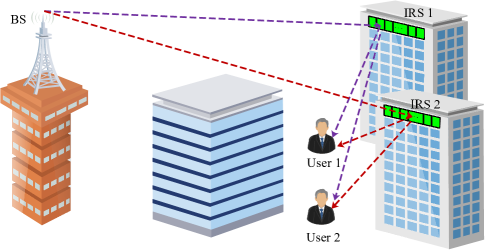
We consider a multi-IRS system, as illustrated in Fig. 1, where one BS with NN antennas communicates with KK single antenna users, each of which is assisted by an IRS with MM reflecting elements. 111 When the number of users is large, it is infeasible to associate each user with a unique IRS. In such scenario, the IRSs can be assigned to users with poor coverage. Alternatively, effective user scheduling protocol can be designed to exploit the benefit of IRSs. We further assume that the direct links between the BS and users do not exist due to blockage or unfavorable propagation environments [7]. The BS is connected with IRSs via low-capacity hardware links so that they can exchange information (e.g. CSI and phase shifts). As in [11, 33], we assume that both the BS and IRSs use uniform linear arrays (ULA). 222 The main reason to use ULA instead of uniform planar array (UPA) is that the simple structure of the ULA helps to get some useful and intuitive insights. In addition, the UPA can be regarded as multiple ULAs. As such, the analytical results obtained for ULA can be readily extended to the UPA structure. Without loss of generality, we assume that the BS is located at the origin of a Cartesian coordinate system, and the ULAs of both the BS and IRSs are along the yy axis.

Refer to caption
Figure 1: Model of the location information aided multi-IRS system with K=2K=2 users assisted by 2 IRSs coated on two buildings. The reflecting elements are represented by green rectangles.

To fully exploit the potential of IRSs, they are usually deployed in desirable locations with LOS paths to both the BS and users. As such, we use angle-domain Rician fading to model the channels between IRSs and the BS or users[8]. Specifically, the channel from the BS to the mm-th IRS can be expressed as

𝐆B2I,m=αB2I,mvB2I,mvB2I,m+1𝐆¯B2I,m+αB2I,m1vB2I,m+1𝐆~B2I,m,\displaystyle{\bf G}_{\text{B2I},m}\!=\!\sqrt{\alpha_{\text{B2I},m}\frac{v_{\text{B2I},m}}{v_{\text{B2I},m}\!+\!1}}\bar{\bf G}_{\text{B2I},m}\!+\!\sqrt{\alpha_{\text{B2I},m}\frac{1}{v_{\text{B2I},m}\!+\!1}}\widetilde{\bf G}_{\text{B2I},m}, (1)

where 𝐆~B2I,mM×N\widetilde{\bf G}_{\text{B2I},m}{\in\mathbb{C}^{M\times N}} is the non-line-of-sight (NLOS) component, whose elements follow the 𝒞𝒩(0,1)\mathcal{CN}\left(0,1\right) distribution, αB2I,m\alpha_{\text{B2I},m} models large-scale fading, and vB2I,mv_{\text{B2I},m} is the Rician K-factor. The LOS component 𝐆¯B2I,mM×N\bar{\bf G}_{\text{B2I},m}{\in\mathbb{C}^{M\times N}} is given by

𝐆¯B2I,m=𝐛(ϑy-B2Ia,m)𝐚T(ϑy-B2I,m),\displaystyle\bar{\bf G}_{\text{B2I},m}={\bf b}\left(\vartheta_{\text{y-B2Ia},m}\right){\bf a}^{T}\left(\vartheta_{\text{y-B2I},m}\right), (2)

where 𝐚(ϑy-B2I,m)N×1{\bf a}\left(\vartheta_{\text{y-B2I},m}\right){\in\mathbb{C}^{N\times 1}} is the array response vector at the BS, with the effective angle of departure (AOD), i.e., the phase difference between two adjacent antennas along the yy axis, given by

ϑy-B2I,m=2πdBSλcosθB2I,msinϕB2I,m,\displaystyle\vartheta_{\text{y-B2I},m}=-\frac{2\pi d_{\text{BS}}}{\lambda}\cos\theta_{\text{B2I},m}\sin\phi_{\text{B2I},m}, (3)

where dBSd_{\text{BS}} is the distance between two adjacent BS antennas, λ\lambda is the carrier wavelength, θB2I,m\theta_{\text{B2I},m} and ϕB2I,m\phi_{\text{B2I},m} are the elevation and azimuth AODs from the BS to the mm-th IRS, respectively.

Similarly, 𝐛(ϑy-B2Ia,m)M×1{\bf b}\left(\vartheta_{\text{y-B2Ia},m}\right){\in\mathbb{C}^{M\times 1}} is the array response vector at the mm-th IRS, where the effective angle of arrival (AOA) is given by

ϑy-B2Ia,m=2πdIRSλcosθB2Ia,msinϕB2Ia,m,\displaystyle\vartheta_{\text{y-B2Ia},m}=\frac{2\pi d_{\text{IRS}}}{\lambda}\cos\theta_{\text{B2Ia},m}\sin\phi_{\text{B2Ia},m}, (4)

where dIRSd_{\text{IRS}} is the distance between two adjacent reflecting elements, θB2Ia,m\theta_{\text{B2Ia},m} and ϕB2Ia,m\phi_{\text{B2Ia},m} are the elevation and azimuth AOAs at the mm-th IRS, respectively. Furthermore, without loss of generality, we assume dBS=dIRS=λ2d_{\text{BS}}=d_{\text{IRS}}=\frac{\lambda}{2}.

Specifically, the nn-th element of 𝐚(ϑ){\bf a}\left(\vartheta\right) and the ll-th element of 𝐛(ϑ){\bf b}\left(\vartheta\right) are given by

an=ejπ(n1)ϑ,n=1,,N,\displaystyle a_{n}=e^{j\pi\left(n-1\right)\vartheta},n=1,...,N, (5)
bl=ejπ(l1)ϑ,l=1,,M.\displaystyle b_{l}=e^{j\pi\left(l-1\right)\vartheta},l=1,...,M. (6)

Similarly, the channel from the mm-th IRS to the kk-th user is given by 𝐠I2U,mkT1×M{\bf g}_{\text{I2U},mk}^{T}{\in\mathbb{C}^{1\times M}}:

𝐠I2U,mkT=αI2U,mkvI2U,mkvI2U,mk+1𝐠¯I2U,mkT+αI2U,mk1vI2U,mk+1𝐠~I2U,mkT,\displaystyle{\bf g}_{\text{I2U},mk}^{T}=\sqrt{\alpha_{\text{I2U},mk}\frac{v_{\text{I2U},mk}}{v_{\text{I2U},mk}+1}}\bar{\bf g}_{\text{I2U},mk}^{T}+\sqrt{\alpha_{\text{I2U},mk}\frac{1}{v_{\text{I2U},mk}+1}}\widetilde{\bf g}_{\text{I2U},mk}^{T}, (7)

with the LOS component 𝐠¯I2U,mkT1×M\bar{\bf g}_{\text{I2U},mk}^{T}{\in\mathbb{C}^{1\times M}} given by

𝐠¯I2U,mkT=𝐛T(ϑy-I2U,mk).\displaystyle\bar{\bf g}_{\text{I2U},mk}^{T}={\bf b}^{T}\left(\vartheta_{\text{y-I2U},mk}\right). (8)

During the downlink data transmission phase, the BS broadcasts the signal

𝐱=i=1K𝐰isi,\displaystyle{\bf x}=\sum\limits_{i=1}^{K}{\bf w}_{i}s_{i}, (9)

where 𝐰iN×1{\bf w}_{i}{\in\mathbb{C}^{N\times 1}} is the transmit beamforming vector and sis_{i} is the symbol for the ii-th user, satisfying 𝔼{|si|2}=1\mathbb{E}\left\{|s_{i}|^{2}\right\}=1.

Then, the signal received at the kk-th user can be expressed as

yk=m=1Ki=1K𝐠I2U,mkT𝚯m𝐆B2I,m𝐰isi+nk,\displaystyle y_{k}=\sum\limits_{m=1}^{K}\sum\limits_{i=1}^{K}{\bf g}_{\text{I2U},mk}^{T}{\mbox{\boldmath$\Theta$}_{m}}{\bf G}_{\text{B2I},m}{\bf w}_{i}s_{i}+n_{k}, (10)

where nk𝒞𝒩(0,σ02)n_{k}\sim\mathcal{CN}\left(0,\sigma_{0}^{2}\right) is the noise at the kk-th user. The phase shift matrix of the mm-th IRS is given by 𝚯m=diag(𝝃m)M×M{\mbox{\boldmath$\Theta$}}_{m}={\text{diag}}\left({\mbox{\boldmath$\xi$}}_{m}\right){\in\mathbb{C}^{M\times M}} with the phase shift beam 𝝃m=[ejϑm,1,,ejϑm,n,,ejϑm,M]TM×1{\mbox{\boldmath$\xi$}}_{m}={[e^{j\vartheta_{m,1}},...,e^{j\vartheta_{m,n}},...,e^{j\vartheta_{m,M}}]}^{T}{\in\mathbb{C}^{M\times 1}}.

III Location based angle information acquisition

To facilitate the design of the transmit beam 𝐰i{\bf w}_{i} and phase shift beam 𝝃m{\mbox{\boldmath$\xi$}}_{m}, CSI of individual channels is necessary. In this section, we exploit the user location information provided by the GPS to obtain angle information of the LOS path. Furthermore, due to the fact that IRS locations are fixed, we assume that they are perfectly known by the BS.

Without loss of generality, we assume the BS is located at the origin (0,0,0)(0,0,0), and the mm-th IRS is located at (xI,m,yI,m,zI,m)(x_{\text{I},m},y_{\text{I},m},z_{\text{I},m}), then the effective AOD from the BS to the mm-th IRS can be computed as

ϑy-B2I,m\displaystyle\vartheta_{\text{y-B2I},m} =yI,mdB2I,m,\displaystyle=-\frac{y_{\text{I},m}}{d_{\text{B2I},m}}, (11)

where dB2I,m=xI,m2+yI,m2+zI,m2d_{\text{B2I},m}=\sqrt{x_{\text{I},m}^{2}+y_{\text{I},m}^{2}+z_{\text{I},m}^{2}} is the distance between the BS and the mm-th IRS.

Similarly, the effective AOA at the mm-th IRS can be calculated as

ϑy-B2Ia,m\displaystyle\vartheta_{\text{y-B2Ia},m} =yI,mdB2I,m.\displaystyle=\frac{y_{\text{I},m}}{d_{\text{B2I},m}}. (12)

Due to user mobility or other unfavorable conditions, the user location information provided by the GPS is imperfect. Specifically, the accurate location of user kk, i.e., (xU,k,yU,k,zU,k)(x_{\text{U},k},y_{\text{U},k},z_{\text{U},k}), is uniformly distributed within a sphere with the radius Υ\Upsilon and center point (x^U,k,y^U,k,z^U,k)(\hat{x}_{\text{U},k},\hat{y}_{\text{U},k},\hat{z}_{\text{U},k}), where (x^U,k,y^U,k,z^U,k)(\hat{x}_{\text{U},k},\hat{y}_{\text{U},k},\hat{z}_{\text{U},k}) is the estimated location of user kk, provided by the GPS.

The mm-th IRS calculates its effective AOD from itself to the kk-th user as

ϑ^y-I2U,mk\displaystyle\hat{\vartheta}_{\text{y-I2U},mk} =yI,my^U,kd^I2U,mk,\displaystyle=\frac{y_{\text{I},m}-\hat{y}_{\text{U},k}}{\hat{d}_{\text{I2U},mk}}, (13)

where d^I2U,mk=(xI,mx^U,k)2+(yI,my^U,k)2+(zI,mz^U,k)2\hat{d}_{\text{I2U},mk}=\sqrt{(x_{\text{I},m}-\hat{x}_{\text{U},k})^{2}+(y_{\text{I},m}-\hat{y}_{\text{U},k})^{2}+(z_{\text{I},m}-\hat{z}_{\text{U},k})^{2}} is the distance between the mm-th IRS and the kk-th user.

Proposition 1

The effective AOD from the mm-th IRS to the kk-th user can be decomposed as

ϑy-I2U,mk=ϑ^y-I2U,mk+ϵy-I2U,mk,\displaystyle\vartheta_{\text{y-I2U},mk}=\hat{\vartheta}_{\text{y-I2U},mk}+\epsilon_{\text{y-I2U},mk}, (14)

where

ϵy-I2U,mk=(ϑ^y-I2U,mk21)ΔyU,k+ϑ^y-I2U,mkϑ^z-I2U,mkΔzU,k+ϑ^y-I2U,mkϑ^z-I2U,mkΔzU,kd^I2U,mk,\displaystyle\epsilon_{\text{y-I2U},mk}=\frac{\left(\hat{\vartheta}^{2}_{\text{y-I2U},mk}-1\right)\Delta y_{\text{U},k}+\hat{\vartheta}_{\text{y-I2U},mk}\hat{\vartheta}_{\text{z-I2U},mk}\Delta z_{\text{U},k}+\hat{\vartheta}_{\text{y-I2U},mk}\hat{\vartheta}_{\text{z-I2U},mk}\Delta z_{\text{U},k}}{\hat{d}_{\text{I2U},mk}}, (15)

where ϑ^x-I2U,mkxI,mx^U,kd^I2U,mk\hat{\vartheta}_{\text{x-I2U},mk}\triangleq\frac{x_{\text{I},m}-\hat{x}_{\text{U},k}}{\hat{d}_{\text{I2U},mk}}, ϑ^z-I2U,mkzI,mz^U,kd^I2U,mk\hat{\vartheta}_{\text{z-I2U},mk}\triangleq\frac{z_{\text{I},m}-\hat{z}_{\text{U},k}}{\hat{d}_{\text{I2U},mk}}, ΔxU,k=xU,kx^U,k\Delta x_{\text{U},k}=x_{\text{U},k}-\hat{x}_{\text{U},k}, ΔyU,k=yU,ky^U,k\Delta y_{\text{U},k}=y_{\text{U},k}-\hat{y}_{\text{U},k} and ΔzU,k=zU,kz^U,k\Delta z_{\text{U},k}=z_{\text{U},k}-\hat{z}_{\text{U},k} are location errors along xx, yy and zz axes, respectively.

Proof:

See Appendix A. ∎

Furthermore, the estimation error ϵy-I2U,mk\epsilon_{\text{y-I2U},mk} has the following distribution.

Theorem 1

The PDF of estimation error ϵy-I2U,mk\epsilon_{\text{y-I2U},mk} is given by

fϵy-I2U,mk(x)=3d^I2U,mk34Υ3Φy-I2U,mk3x2+3d^I2U,mk4ΥΦy-I2U,mk1,|x|Υd^I2U,mkΦy-I2U,mk,\displaystyle f_{\epsilon_{\text{y-I2U},mk}}\left(x\right)=-\frac{3{\hat{d}}^{3}_{\text{I2U},mk}}{4\Upsilon^{3}}{\Phi}^{-3}_{\text{y-I2U},mk}x^{2}+\frac{3{\hat{d}}_{\text{I2U},mk}}{4\Upsilon}{\Phi}^{-1}_{\text{y-I2U},mk},\ |x|\leq\frac{\Upsilon}{\hat{d}_{\text{I2U},mk}}{\Phi}_{\text{y-I2U},mk}, (16)

where

Φy-I2U,mk(ϑ^y-I2U,mk21)2+ϑ^y-I2U,mk2ϑ^z-I2U,mk2+ϑ^y-I2U,mk2ϑ^x-I2U,mk2.\displaystyle\Phi_{\text{y-I2U},mk}\triangleq\sqrt{{\left(\hat{\vartheta}^{2}_{\text{y-I2U},mk}-1\right)}^{2}+\hat{\vartheta}^{2}_{\text{y-I2U},mk}\hat{\vartheta}^{2}_{\text{z-I2U},mk}+\hat{\vartheta}^{2}_{\text{y-I2U},mk}\hat{\vartheta}^{2}_{\text{x-I2U},mk}}. (17)

The mean and variance of ϵy-I2U,mk\epsilon_{\text{y-I2U},mk} are given by

μy-I2U,mk=𝔼{ϵy-I2U,mk}=0,\displaystyle\mu_{\text{y-I2U},mk}=\mathbb{E}\left\{\epsilon_{\text{y-I2U},mk}\right\}=0, (18)
σy-I2U,mk2=𝔼{ϵy-I2U,mk2}=Υ25d^I2U,mk2Φy-I2U,mk2.\displaystyle\sigma_{\text{y-I2U},mk}^{2}=\mathbb{E}\left\{\epsilon^{2}_{\text{y-I2U},mk}\right\}=\frac{\Upsilon^{2}}{5\hat{d}^{2}_{\text{I2U},mk}}\Phi^{2}_{\text{y-I2U},mk}. (19)
Proof:

See Appendix B. ∎

Remark 1

Theorem 1 indicates that angle estimation accuracy is greatly affected by the user location uncertainty as well as the distance between the IRS and the user. Specifically, the variance of the angle estimation error is proportional to the ratio Υ2d^I2U,mk2\frac{\Upsilon^{2}}{\hat{d}^{2}_{\text{I2U},mk}}, implying that increasing the distance between the IRS and the user can compensate for the adverse effect of user location uncertainty.

IV Design of transmit and phase shift beams

After obtaining the angle information, the BS uses the estimated angles to design transmit and phase shift beams. Since transmit and phase shift beams are coupled, the resultant optimization problem is non-convex, hence the global optimal solution is in general intractable. As such, many sub-optimal algorithms have been proposed such as alternating optimization. However, due to the large number of reflecting elements, the computational complexity of these algorithms is very high. Motivated by this, instead of aiming for the global optimal solution, we perform low-complexity local optimization at the BS and each IRS, separately, where closed-form solutions can be obtained.

Specifically, the BS utilizes the angle information of the BS-IRS link to design the transmit beam. Without loss of generality, we assume the kk-th user is assisted by the kk-th IRS. Thus, the transmit beam for the kk-th user should be aligned to the kk-th IRS. As such, the transmit beam is designed as

𝐰k=ηkρdN𝐚B2I,k,\displaystyle{\bf w}_{k}=\sqrt{\frac{\eta_{k}\rho_{d}}{N}}{\bf{a}}_{\text{B2I},k}^{*}, (20)

where 𝐚B2I,k𝐚(ϑy-B2I,k)N×1{\bf{a}}_{\text{B2I},k}\triangleq{\bf a}\left(\vartheta_{\text{y-B2I},k}\right){\in\mathbb{C}^{N\times 1}}, ρd\rho_{d} is the transmit power of the BS and 0<ηk<10<\eta_{k}<1 is the power control coefficient.

The estimated angle information of the IRS-user link is used to design the phase shift beam. For the kk-th user, we aim to maximize its received signal via the kk-th IRS by optimizing the phase shift beam 𝝃k\mbox{\boldmath$\xi$}_{k}. Specifically, the optimization problem is formulated as

max𝚯k|𝐠I2U,kkT𝚯k𝐆B2I,k𝐰k|2,s.t.|[𝚯k]ii|=1,i=1,,M.\displaystyle\begin{array}[]{ll}\max\limits_{{\mbox{\boldmath$\Theta$}}_{k}}&\left|{\bf g}_{\text{I2U},kk}^{T}{\mbox{\boldmath$\Theta$}_{k}}{\bf G}_{\text{B2I},k}{\bf w}_{k}\right|^{2},\\ \operatorname{s.t.}&\begin{array}[t]{lll}\left|{\left[{\bf\Theta}_{k}\right]}_{ii}\right|=1,i=1,...,M.\end{array}\end{array} (24)

According to the rule that 𝐄T𝐗𝐅=𝐱T(𝐄𝐅){\bf E}^{T}{\bf X}{\bf F}={\bf x}^{T}\left({\bf E}\odot{\bf F}\right) with 𝐗=diag(𝐱){\bf X}={\text{diag}}\left({\bf x}\right), we have

𝐠I2U,kkT𝚯k𝐆B2I,k𝐰k=𝝃kT(𝐠I2U,kk𝐆B2I,k𝐰k)=𝝃kT(𝐠I2U,kk𝐛B2I,k)𝐚B2I,kT𝐰k,\displaystyle{\bf g}_{\text{I2U},kk}^{T}{\mbox{\boldmath$\Theta$}_{k}}{\bf G}_{\text{B2I},k}{\bf w}_{k}={\mbox{\boldmath$\xi$}_{k}^{T}}\left({\bf g}_{\text{I2U},kk}\odot{\bf G}_{\text{B2I},k}{\bf w}_{k}\right)={\mbox{\boldmath$\xi$}_{k}^{T}}\left({\bf g}_{\text{I2U},kk}\odot{\bf b}_{\text{B2I},k}\right){\bf a}^{T}_{\text{B2I},k}{\bf w}_{k}, (25)

where 𝐛B2I,k𝐛(ϑy-B2Ia,k)M×1{\bf b}_{\text{B2I},k}\triangleq{\bf b}\left(\vartheta_{\text{y-B2Ia},k}\right){\in\mathbb{C}^{M\times 1}}.

Based on the above equation, the objective function in (24) becomes

|𝝃kT(𝐠I2U,kk𝐛B2I,k)|2|𝐚B2I,kT𝐰k|2.\displaystyle\left|{\mbox{\boldmath$\xi$}_{k}^{T}}\left({\bf g}_{\text{I2U},kk}\odot{\bf b}_{\text{B2I},k}\right)\right|^{2}\left|{\bf a}^{T}_{\text{B2I},k}{\bf w}_{k}\right|^{2}. (26)

Noticing that |𝐚B2I,kT𝐰k|2\left|{\bf a}^{T}_{\text{B2I},k}{\bf w}_{k}\right|^{2} is a constant independent of 𝝃k{\mbox{\boldmath$\xi$}}_{k} , the optimization problem is equivalent to

max𝝃kT|𝝃kT(𝐠I2U,kk𝐛B2I,k)|2,s.t.|[𝝃k]i|=1,i=1,,M.\displaystyle\begin{array}[]{ll}\max\limits_{{\mbox{\boldmath$\xi$}}_{k}^{T}}&\left|{\mbox{\boldmath$\xi$}_{k}^{T}}\left({\bf g}_{\text{I2U},kk}\odot{\bf b}_{\text{B2I},k}\right)\right|^{2},\\ \operatorname{s.t.}&\begin{array}[t]{lll}\left|\left[{\mbox{\boldmath$\xi$}}_{k}\right]_{i}\right|=1,i=1,...,M.\end{array}\end{array} (30)

Obviously, the solution for the above optimization problem is

𝝃k=(𝐠I2U,kk𝐛B2I,k).\displaystyle{\mbox{\boldmath$\xi$}}_{k}=\left({\bf g}_{\text{I2U},kk}\odot{\bf b}_{\text{B2I},k}\right)^{*}. (31)

Using the estimated angles, we design the phase shift beam as

𝝃k=(𝐠¯^I2U,kk𝐛B2I,k),\displaystyle{\mbox{\boldmath$\xi$}}_{k}=\left({\hat{\bar{\bf g}}}_{\text{I2U},kk}\odot{\bf b}_{\text{B2I},k}\right)^{*}, (32)

where 𝐠¯^I2U,mk=𝐛(ϑ^y-I2U,mk)M×1{\hat{\bar{\bf g}}}_{\text{I2U},mk}={\bf b}\left(\hat{\vartheta}_{\text{y-I2U},mk}\right){\in\mathbb{C}^{M\times 1}}.

V Achievable Rate Analysis

In this section, we present a detailed investigation on the achievable rate of the multi-IRS system. Without loss of generality, let us focus on the achievable rate of the kk-th user. We consider the realistic case where the kk-th user does not have access to the instantaneous CSI of the effective channel gain. As such, we can rewrite yk{{y}}_{k} as

yk=𝔼{𝐠kT𝐰k}skdesired signal+(𝐠kT𝐰k𝔼{𝐠kT𝐰k})skleakage signal+𝐠kTikK𝐰isiinter-user interference+nknoise,\displaystyle y_{k}=\underbrace{\mathbb{E}\left\{{\bf g}_{k}^{T}{\bf w}_{k}\right\}s_{k}}_{\text{desired signal}}+\underbrace{{\left({\bf g}_{k}^{T}{\bf w}_{k}-\mathbb{E}\left\{{\bf g}_{k}^{T}{\bf w}_{k}\right\}\right)}s_{k}}_{\text{leakage signal}}+\underbrace{{\bf g}_{k}^{T}\sum\limits_{i\neq k}^{K}{\bf w}_{i}s_{i}}_{\text{inter-user interference}}+\underbrace{n_{k}}_{\text{noise}}, (33)

where we define the equivalent channel of the kk-the user as

𝐠kT=m=1K𝐠I2U,mkT𝚯m𝐆B2I,m.\displaystyle{\bf g}_{k}^{T}=\sum\limits_{m=1}^{K}{\bf g}_{\text{I2U},mk}^{T}{\mbox{\boldmath$\Theta$}_{m}}{\bf G}_{\text{B2I},m}. (34)

Invoking the result in [34], the achievable rate of the kk-th user is given by

Rk=log2(1+AkBk+ikKCk,i+σ02),\displaystyle R_{k}=\log_{2}\left(1+\frac{A_{k}}{B_{k}+\sum\limits_{i\neq k}^{K}C_{k,i}+\sigma_{0}^{2}}\right), (35)

where

Ak|𝔼{𝐠kT𝐰k}|2,\displaystyle A_{k}\triangleq{\left|\mathbb{E}\left\{{\bf g}_{k}^{T}{\bf w}_{k}\right\}\right|}^{2}, (36)
Bk𝔼{|𝐠kT𝐰k𝔼{𝐠kT𝐰k}|2},\displaystyle B_{k}\triangleq\mathbb{E}\left\{{\left|{{{\bf g}_{k}^{T}{\bf w}_{k}-\mathbb{E}\left\{{\bf g}_{k}^{T}{\bf w}_{k}\right\}}}\right|}^{2}\right\}, (37)
Ck,i𝔼{|𝐠kT𝐰i|2},\displaystyle C_{k,i}\triangleq\mathbb{E}\left\{{\left|{{\bf g}_{k}^{T}{\bf w}_{i}}\right|}^{2}\right\}, (38)

denote the desired signal power, leakage power and interference, respectively.

To derive the expression of RkR_{k}, we first give the following Lemma:

Lemma 1

The correlation coefficient between ϱI2U,mk,sejπ(s1)ϵy-I2U,mk\varrho_{\text{I2U},mk,s}\triangleq e^{j\pi\left(s-1\right)\epsilon_{\text{y-I2U},mk}} and ϱI2U,nk,l,nm\varrho_{\text{I2U},nk,l},n\neq m, is given by

ζy-I2U,mk,nk,sl𝔼{ϱI2U,mk,sϱI2U,nk,l},\displaystyle\zeta_{\text{y-I2U},mk,nk,sl}\triangleq\mathbb{E}\left\{\varrho_{\text{I2U},mk,s}\varrho_{\text{I2U},nk,l}^{*}\right\}, (39)
={1,s=1andl=13ϖk,mn,sl2(sinϖk,mn,slϖk,mn,slcosϖk,mn,sl),else\displaystyle=\begin{cases}1,&s=1\ \text{and}\ l=1\\ \frac{3}{\varpi_{k,mn,sl}^{2}}\left(\frac{\sin\varpi_{k,mn,sl}}{\varpi_{k,mn,sl}}-\cos\varpi_{k,mn,sl}\right),&\text{else}\end{cases}

where

ϖk,mn,slπΥak,mn,sl2+bk,mn,sl2+ck,mn,sl2,\displaystyle\varpi_{k,mn,sl}\triangleq\pi\Upsilon\sqrt{a^{2}_{k,mn,sl}+b^{2}_{k,mn,sl}+c^{2}_{k,mn,sl}}, (40)
ak,mn,sl(s1)ϑ^y-I2U,mk21d^I2U,mk(l1)ϑ^y-I2U,nk21d^I2U,nk,\displaystyle a_{k,mn,sl}\triangleq\left(s-1\right)\frac{\hat{\vartheta}^{2}_{\text{y-I2U},mk}-1}{\hat{d}_{\text{I2U},mk}}-\left(l-1\right)\frac{\hat{\vartheta}^{2}_{\text{y-I2U},nk}-1}{\hat{d}_{\text{I2U},nk}}, (41)
bk,mn,sl(s1)ϑ^y-I2U,mkϑ^z-I2U,mkd^I2U,mk(l1)ϑ^y-I2U,nkϑ^z-I2U,nkd^I2U,nk,\displaystyle b_{k,mn,sl}\triangleq\left(s-1\right)\frac{\hat{\vartheta}_{\text{y-I2U},mk}\hat{\vartheta}_{\text{z-I2U},mk}}{\hat{d}_{\text{I2U},mk}}-\left(l-1\right)\frac{\hat{\vartheta}_{\text{y-I2U},nk}\hat{\vartheta}_{\text{z-I2U},nk}}{\hat{d}_{\text{I2U},nk}}, (42)
ck,mn,sl(s1)ϑ^y-I2U,mkϑ^x-I2U,mkd^I2U,mk(l1)ϑ^y-I2U,nkϑ^x-I2U,nkd^I2U,nk.\displaystyle c_{k,mn,sl}\triangleq\left(s-1\right)\frac{\hat{\vartheta}_{\text{y-I2U},mk}\hat{\vartheta}_{\text{x-I2U},mk}}{\hat{d}_{\text{I2U},mk}}-\left(l-1\right)\frac{\hat{\vartheta}_{\text{y-I2U},nk}\hat{\vartheta}_{\text{x-I2U},nk}}{\hat{d}_{\text{I2U},nk}}. (43)
Proof:

See Appendix C. ∎

Theorem 2

The achievable rate of the kk-th user is given by

Rk=log2(1+AkBk+ikKCk,i+σ02),\displaystyle R_{k}=\log_{2}\left(1+\frac{A_{k}}{B_{k}+\sum\limits_{i\neq k}^{K}C_{k,i}+\sigma_{0}^{2}}\right), (44)

where

Ak=ηkρdN|m=1Ks=1MβB2I2U,mk𝐚B2I,mT𝐚B2I,kζy-I2U,mk,s[𝐠¯^I2U,mk]s[𝐠¯^I2U,mm]s|2,\displaystyle A_{k}=\frac{\eta_{k}\rho_{d}}{N}\left|\sum\limits_{m=1}^{K}\sum\limits_{s=1}^{M}\sqrt{\beta_{\text{B2I2U},mk}}{\bf a}^{T}_{\text{B2I},m}{\bf a}_{\text{B2I},k}^{*}\zeta_{\text{y-I2U},mk,s}{\left[{\hat{\bar{\bf g}}}_{\text{I2U},mk}\right]}_{s}{\left[{\hat{\bar{\bf g}}}_{\text{I2U},mm}\right]}_{s}^{*}\right|^{2}, (45)
Ck,i=ηiρdNm=1K(MβB2I2U,mkvI2U,mk|𝐚B2I,mT𝐚B2I,i|2+MNβB2I2U,mkvB2I,mvI2U,mk+MNβB2I2U,mkvB2I,m)\displaystyle C_{k,i}=\frac{\eta_{i}\rho_{d}}{N}\sum\limits_{m=1}^{K}\left(M\frac{\beta_{\text{B2I2U},mk}}{v_{\text{I2U},mk}}\left|{\bf a}^{T}_{\text{B2I},m}{\bf a}_{\text{B2I},i}^{*}\right|^{2}+MN\frac{\beta_{\text{B2I2U},mk}}{v_{\text{B2I},m}v_{\text{I2U},mk}}+MN\frac{\beta_{\text{B2I2U},mk}}{v_{\text{B2I},m}}\right) (46)
+ηiρdNm=1Ks=1Ml=1MβB2I2U,mk|𝐚B2I,mT𝐚B2I,i|2ζy-I2U,mk,sl[𝐠¯^I2U,mk]s[𝐠¯^I2U,mm]s[𝐠¯^I2U,mk]l[𝐠¯^I2U,mm]l\displaystyle+\frac{\eta_{i}\rho_{d}}{N}\sum\limits_{m=1}^{K}\sum\limits_{s=1}^{M}\sum\limits_{l=1}^{M}\beta_{\text{B2I2U},mk}\left|{\bf a}^{T}_{\text{B2I},m}{\bf a}_{\text{B2I},i}^{*}\right|^{2}\zeta_{\text{y-I2U},mk,sl}{\left[{\hat{\bar{\bf g}}}_{\text{I2U},mk}\right]}_{s}{\left[{\hat{\bar{\bf g}}}_{\text{I2U},mm}\right]}_{s}^{*}{\left[{\hat{\bar{\bf g}}}_{\text{I2U},mk}\right]}_{l}^{*}{\left[{\hat{\bar{\bf g}}}_{\text{I2U},mm}\right]}_{l}
+ηiρdNm=1KnmKs=1Ml=1M𝐚B2I,mT𝐚B2I,iβB2I2U,mk𝐚B2I,nH𝐚B2I,iβB2I2U,nk\displaystyle+\frac{\eta_{i}\rho_{d}}{N}\sum\limits_{m=1}^{K}\sum\limits_{n\neq m}^{K}\sum\limits_{s=1}^{M}\sum\limits_{l=1}^{M}{\bf a}^{T}_{\text{B2I},m}{\bf a}_{\text{B2I},i}^{*}\sqrt{\beta_{\text{B2I2U},mk}}{\bf a}^{H}_{\text{B2I},n}{\bf a}_{\text{B2I},i}\sqrt{\beta_{\text{B2I2U},nk}}
×ζy-I2U,mk,nk,sl[𝐠¯^I2U,mk]s[𝐠¯^I2U,mm]s[𝐠¯^I2U,nk]l[𝐠¯^I2U,nn]l,\displaystyle\times\zeta_{\text{y-I2U},mk,nk,sl}{\left[{\hat{\bar{\bf g}}}_{\text{I2U},mk}\right]}_{s}{\left[{\hat{\bar{\bf g}}}_{\text{I2U},mm}\right]}_{s}^{*}{\left[{\hat{\bar{\bf g}}}_{\text{I2U},nk}\right]}_{l}^{*}{\left[{\hat{\bar{\bf g}}}_{\text{I2U},nn}\right]}_{l},
Bk=Ck,kAk,\displaystyle B_{k}=C_{k,k}-A_{k}, (47)

where βB2I2U,mkαB2I,mvB2I,mαI2U,mkvI2U,mk(vB2I,m+1)(vI2U,mk+1)\beta_{\text{B2I2U},mk}\triangleq\frac{\alpha_{\text{B2I},m}v_{\text{B2I},m}\alpha_{\text{I2U},mk}v_{\text{I2U},mk}}{(v_{\text{B2I},m}+1)(v_{\text{I2U},mk}+1)} and

ζy-I2U,mk,s=\displaystyle\zeta_{\text{y-I2U},mk,s}\!=\! {3ϖy-I2U,mk,s2(sinϖy-I2U,mk,sϖy-I2U,mk,scosϖy-I2U,mk,s)s11s=1,\displaystyle\begin{cases}\frac{3}{\varpi_{\text{y-I2U},mk,s}^{2}}\left(\frac{\sin\varpi_{\text{y-I2U},mk,s}}{\varpi_{\text{y-I2U},mk,s}}-\cos\varpi_{\text{y-I2U},mk,s}\right)&s\!\neq\!1\\ 1&s\!=\!1\end{cases}, (48)
ζy-I2U,mk,sl=\displaystyle\zeta_{\text{y-I2U},mk,sl}\!=\! {3ϖy-I2U,mk,sl2(sinϖy-I2U,mk,slϖy-I2U,mk,slcosϖy-I2U,mk,sl)sl1s=l,\displaystyle\begin{cases}\frac{3}{\varpi_{\text{y-I2U},mk,sl}^{2}}\left(\frac{\sin\varpi_{\text{y-I2U},mk,sl}}{\varpi_{\text{y-I2U},mk,sl}}-\cos\varpi_{\text{y-I2U},mk,sl}\right)&s\!\neq\!l\\ 1&s\!=\!l\end{cases}, (49)

with ϖy-I2U,mk,sπ(s1)Φy-I2U,mkΥd^I2U,mk\varpi_{\text{y-I2U},mk,s}\triangleq\frac{\pi\left(s-1\right){\Phi}_{\text{y-I2U},mk}\Upsilon}{{\hat{d}}_{\text{I2U},mk}} and ϖy-I2U,mk,slπ(sl)Φy-I2U,mkΥd^I2U,mk\varpi_{\text{y-I2U},mk,sl}\triangleq\frac{\pi\left(s-l\right){\Phi}_{\text{y-I2U},mk}\Upsilon}{{\hat{d}}_{\text{I2U},mk}}.

Proof:

See Appendix D. ∎

Theorem 2 presents a closed-form expression for the achievable rate, which quantifies the impacts of some key parameters, such as antenna number, user number, the number of reflecting elements, Rician K-factor and user location uncertainty. For instance, RkR_{k} is an increasing function with respect to the Rician K-factor, because a small Rician K-factor implies more interference caused by NLOS paths. Also, increasing the number of users would degrade the individual rate, due to stronger inter-user interference. In addition, as Υ\Upsilon becomes larger, ζy-I2U,mk,s0\zeta_{\text{y-I2U},mk,s}\to 0 and thus RkR_{k} gradually goes to zero, indicating that the achievable rate would significantly degrade as user location uncertainty becomes larger. Moreover, we can see that Ck,iC_{k,i} increases with the correlation coefficient between 𝐚B2I,i{\bf a}_{\text{B2I},i} and 𝐚B2I,m,mi{\bf a}_{\text{B2I},m},m\neq i, implying that IRSs should be deployed at distinct directions relative to the BS to reduce the interference from multiple IRSs. Ideally, it is desired that 𝐚B2I,mT𝐚B2I,i0,mi{\bf a}_{\text{B2I},m}^{T}{\bf a}_{\text{B2I},i}^{*}\to 0,m\neq i.

We now consider some special cases, where simplified expressions are available.

V-A Ideal directions (relative to the BS) of IRSs

Proposition 2

To reduce the interference from multiple IRSs, ideally the directions (relative to the BS) of any two IRSs should satisfy |ϑB2I,mϑB2I,i|=2nN,im,n{1,,N1}\left|\vartheta_{\text{B2I},m}-\vartheta_{\text{B2I},i}\right|=\frac{2n}{N},i\neq m,n\in\{1,...,N-1\}.

Proof:

Let 𝐚B2I,mT𝐚B2I,i=0,mi{\bf a}_{\text{B2I},m}^{T}{\bf a}_{\text{B2I},i}^{*}=0,m\neq i. Noticing that

𝐚B2I,mT𝐚B2I,i=sinNπ(ϑB2I,mϑB2I,i)2sinπ(ϑB2I,mϑB2I,i)2ejπ(N1)ϑB2I,mϑB2I,i2,\displaystyle{\bf a}_{\text{B2I},m}^{T}{\bf a}_{\text{B2I},i}=\frac{\sin\frac{N\pi(\vartheta_{\text{B2I},m}-\vartheta_{\text{B2I},i})}{2}}{\sin\frac{\pi(\vartheta_{\text{B2I},m}-\vartheta_{\text{B2I},i})}{2}}e^{j\pi(N-1)\frac{\vartheta_{\text{B2I},m}-\vartheta_{\text{B2I},i}}{2}}, (50)

we can obtain the desired result. ∎

Proposition 2 indicates that it is possible to eliminate the interference from other IRSs by deploying them at proper directions (relative to the BS).

Corollary 1

With ideal directions (relative to the BS) of IRSs, i.e., 𝐚B2I,mT𝐚B2I,i0,mi{\bf a}_{\text{B2I},m}^{T}{\bf a}_{\text{B2I},i}\to 0,m\neq i, the achievable rate is given by

Rk=log2(1+AkBk+ikKCk,i+σ02),\displaystyle R_{k}=\log_{2}\left(1+\frac{A_{k}}{B_{k}+\sum\limits_{i\neq k}^{K}C_{k,i}+\sigma_{0}^{2}}\right), (51)

where

Ak=NηkρdβB2I2U,kk|s=1Mζy-I2U,kk,s|2,\displaystyle A_{k}=N\eta_{k}\rho_{d}\beta_{\text{B2I2U},kk}\left|\sum\limits_{s=1}^{M}\zeta_{\text{y-I2U},kk,s}\right|^{2}, (52)
Ck,i=NMηiρdβB2I2U,ikvI2U,ik+Mηiρdm=1K(βB2I2U,mkvB2I,mvI2U,mk+βB2I2U,mkvB2I,m)\displaystyle C_{k,i}=NM\eta_{i}\rho_{d}\frac{\beta_{\text{B2I2U},ik}}{v_{\text{I2U},ik}}+M\eta_{i}\rho_{d}\sum\limits_{m=1}^{K}\left(\frac{\beta_{\text{B2I2U},mk}}{v_{\text{B2I},m}v_{\text{I2U},mk}}+\frac{\beta_{\text{B2I2U},mk}}{v_{\text{B2I},m}}\right) (53)
+Nηiρds=1Ml=1MβB2I2U,ikζy-I2U,ik,sl[𝐠¯^I2U,ik]s[𝐠¯^I2U,ii]s[𝐠¯^I2U,ik]l[𝐠¯^I2U,ii]l,\displaystyle+N\eta_{i}\rho_{d}\sum\limits_{s=1}^{M}\sum\limits_{l=1}^{M}\beta_{\text{B2I2U},ik}\zeta_{\text{y-I2U},ik,sl}{\left[{\hat{\bar{\bf g}}}_{\text{I2U},ik}\right]}_{s}{\left[{\hat{\bar{\bf g}}}_{\text{I2U},ii}\right]}_{s}^{*}{\left[{\hat{\bar{\bf g}}}_{\text{I2U},ik}\right]}_{l}^{*}{\left[{\hat{\bar{\bf g}}}_{\text{I2U},ii}\right]}_{l},
Bk=NMηkρdβB2I2U,kkvI2U,kk+Mηkρdm=1K(βB2I2U,mkvB2I,mvI2U,mk+βB2I2U,mkvB2I,m)\displaystyle B_{k}=NM\eta_{k}\rho_{d}\frac{\beta_{\text{B2I2U},kk}}{v_{\text{I2U},kk}}+M\eta_{k}\rho_{d}\sum\limits_{m=1}^{K}\left(\frac{\beta_{\text{B2I2U},mk}}{v_{\text{B2I},m}v_{\text{I2U},mk}}+\frac{\beta_{\text{B2I2U},mk}}{v_{\text{B2I},m}}\right) (54)
+NηkρdβB2I2U,kks=1Ml=1M(ζy-I2U,kk,slζy-I2U,kk,sζy-I2U,kk,l).\displaystyle+N\eta_{k}\rho_{d}\beta_{\text{B2I2U},kk}\sum\limits_{s=1}^{M}\sum\limits_{l=1}^{M}\left(\zeta_{\text{y-I2U},kk,sl}-\zeta_{\text{y-I2U},kk,s}\zeta_{\text{y-I2U},kk,l}^{*}\right).
Proof:

Starting from Theorem 2, we can obtain the desired result. ∎

From Corollary 1, we can observe that the desire signal AkA_{k} is proportional to βB2I2U,kk\beta_{\text{B2I2U},kk}, indicating that a user should be associated with the nearest IRS. Besides, it can be seen that Ck,iC_{k,i} increases proportionally with βB2I2U,ki,ik\beta_{\text{B2I2U},ki},i\neq k, which implies that the interference from other IRSs (with indexes iki\neq k) would be reduced if they are far away from the kk-th user. According to the above two observations, we conclude that IRSs should be deployed far away from each other. Moreover, we can see that the desired signal power is proportional to the number of BS antennas, indicating the benefit of applying multiple antennas.

V-B Perfect information of user locations

Corollary 2

With perfect user location information, i.e., Υ0\Upsilon\to 0, the achievable rate is given by

Rk=log2(1+AkBk+ikKCk,i+σ02),\displaystyle R_{k}=\log_{2}\left(1+\frac{A_{k}}{B_{k}+\sum\limits_{i\neq k}^{K}C_{k,i}+\sigma_{0}^{2}}\right), (55)

where

Ak=NM2ηkρdβB2I2U,kk,\displaystyle A_{k}=NM^{2}\eta_{k}\rho_{d}\beta_{\text{B2I2U},kk}, (56)
Ck,i=NMηiρdβB2I2U,ikvI2U,ik+Mηiρdm=1K(βB2I2U,mkvB2I,mvI2U,mk+βB2I2U,mkvB2I,m)\displaystyle C_{k,i}=NM\eta_{i}\rho_{d}\frac{\beta_{\text{B2I2U},ik}}{v_{\text{I2U},ik}}+M\eta_{i}\rho_{d}\sum\limits_{m=1}^{K}\left(\frac{\beta_{\text{B2I2U},mk}}{v_{\text{B2I},m}v_{\text{I2U},mk}}+\frac{\beta_{\text{B2I2U},mk}}{v_{\text{B2I},m}}\right) (57)
+NηiρdβB2I2U,ik|sinMπ(ϑ^I2U,ikϑ^I2U,ii)2sinπ(ϑ^I2U,ikϑ^I2U,ii)2|2,\displaystyle+N\eta_{i}\rho_{d}\beta_{\text{B2I2U},ik}\left|\frac{\sin\frac{M\pi(\hat{\vartheta}_{\text{I2U},ik}-\hat{\vartheta}_{\text{I2U},ii})}{2}}{\sin\frac{\pi(\hat{\vartheta}_{\text{I2U},ik}-\hat{\vartheta}_{\text{I2U},ii})}{2}}\right|^{2},
Bk=NMηkρdβB2I2U,kkvI2U,kk+Mηkρdm=1K(βB2I2U,mkvB2I,mvI2U,mk+βB2I2U,mkvB2I,m).\displaystyle B_{k}=NM\eta_{k}\rho_{d}\frac{\beta_{\text{B2I2U},kk}}{v_{\text{I2U},kk}}+M\eta_{k}\rho_{d}\sum\limits_{m=1}^{K}\left(\frac{\beta_{\text{B2I2U},mk}}{v_{\text{B2I},m}v_{\text{I2U},mk}}+\frac{\beta_{\text{B2I2U},mk}}{v_{\text{B2I},m}}\right). (58)
Proof:

We first consider the following limit:

limϖ0ζ=limϖ03ϖ2(sinϖϖcosϖ).\displaystyle\lim_{\varpi\to 0}\zeta=\lim_{\varpi\to 0}\frac{3}{\varpi^{2}}\left(\frac{\sin\varpi}{\varpi}-\cos\varpi\right). (59)

Using the Taylor expansions of sinϖ\sin\varpi and cosϖ\cos\varpi at ϖ=0\varpi=0, we have

limϖ0sinϖ=ϖ16ϖ3,\displaystyle\lim_{\varpi\to 0}\sin\varpi=\varpi-\frac{1}{6}\varpi^{3}, (60)
limϖ0cosϖ=112ϖ2,\displaystyle\lim_{\varpi\to 0}\cos\varpi=1-\frac{1}{2}\varpi^{2}, (61)

based on which, (59) can be expressed as

limϖ0ζ=limϖ03ϖ2{ϖ16ϖ3ϖ(112ϖ2)}=1.\displaystyle\lim_{\varpi\to 0}\zeta=\lim_{\varpi\to 0}\frac{3}{\varpi^{2}}\left\{\frac{\varpi-\frac{1}{6}\varpi^{3}}{\varpi}-\left(1-\frac{1}{2}\varpi^{2}\right)\right\}=1. (62)

As Υ\Upsilon\to\infty, ϖy-I2U,mk,s0\varpi_{\text{y-I2U},mk,s}\to 0, ϖy-I2U,mk,sl0\varpi_{\text{y-I2U},mk,sl}\to 0 and ϖk,mn,sl0\varpi_{k,mn,sl}\to 0.

Invoking (62), we have ζy-I2U,mk,s1\zeta_{\text{y-I2U},mk,s}\to 1, ζy-I2U,mk,sl1\zeta_{\text{y-I2U},mk,sl}\to 1 and ζy-I2U,mk,nk,sl1\zeta_{\text{y-I2U},mk,nk,sl}\to 1.

As such, simplifying the achievable rate given by Corollary 1 yields the desired result. ∎

Corollary 2 shows that as Υ\Upsilon goes to zero, the achievable rate converges to a limit, due to the vanished angle estimation error. Moreover, we can see that the desired signal power becomes proportional to NM2NM^{2}. The NN-fold gain is achieved by the transmit beamforming, while the M2M^{2}-fold gain comes from the fact that the IRS not only achieves the phase shift beamforming gain in the IRS-user link, but also captures an inherent aperture gain by collecting more signal power in the BS-IRS link.

To gain more insights, we now look into some asymptotic regime.

V-B1 A large number of reflecting elements

Corollary 3

With a large number of reflecting elements, i.e., MM\to\infty, the achievable rate is given by

Rk=log2(1+NMηkβB2I2U,kkNi=1KηiβB2I2U,ikvI2U,ik+m=1K(βB2I2U,mkvB2I,mvI2U,mk+βB2I2U,mkvB2I,m)).\displaystyle R_{k}=\log_{2}\left(1+\frac{NM\eta_{k}\beta_{\text{B2I2U},kk}}{N\sum\limits_{i=1}^{K}\eta_{i}\frac{\beta_{\text{B2I2U},ik}}{v_{\text{I2U},ik}}+\sum\limits_{m=1}^{K}\left(\frac{\beta_{\text{B2I2U},mk}}{v_{\text{B2I},m}v_{\text{I2U},mk}}+\frac{\beta_{\text{B2I2U},mk}}{v_{\text{B2I},m}}\right)}\right). (63)
Proof:

Starting from Corollary 2 and neglecting the insignificant terms, the desired result can be obtained. ∎

From Corollary 3, we can see that the achievable rate is mainly determined by the number of reflecting elements, antenna number, Rician K-factor and power allocation coefficients. For instance, the SINR is proportional to the number of reflecting elements, indicating the benefit of deploying a large number of reflecting elements. However, in practice, to control the cost of IRS deployment, the number of reflecting elements can not be infinite. Since the achievable rate grows logarithmically with the number of reflecting elements, the benefit of increasing the number of reflecting elements becomes less significant in the regime with large number of reflecting elements. Thus, caution should be exercised for choosing the number of IRS elements in order to achieve a fine balance between the deployment cost and the achievable rate.

Also, the achievable rate is an increasing function with respect to the number of BS antennas.

V-B2 A large number of antennas

Corollary 4

With a large number of antennas, i.e., NN\to\infty, the achievable rate is given by

Rk=log2(1+M2ηkβB2I2U,kkMi=1KηiβB2I2U,ikvI2U,ik+ikKηiβB2I2U,ik|sinMπ(ϑ^I2U,ikϑ^I2U,ii)2sinπ(ϑ^I2U,ikϑ^I2U,ii)2|2).\displaystyle R_{k}=\log_{2}\left(1+\frac{M^{2}\eta_{k}\beta_{\text{B2I2U},kk}}{M\sum\limits_{i=1}^{K}\eta_{i}\frac{\beta_{\text{B2I2U},ik}}{v_{\text{I2U},ik}}+\sum\limits_{i\neq k}^{K}\eta_{i}\beta_{\text{B2I2U},ik}\left|\frac{\sin\frac{M\pi(\hat{\vartheta}_{\text{I2U},ik}-\hat{\vartheta}_{\text{I2U},ii})}{2}}{\sin\frac{\pi(\hat{\vartheta}_{\text{I2U},ik}-\hat{\vartheta}_{\text{I2U},ii})}{2}}\right|^{2}}\right). (64)
Proof:

Starting from Corollary 2 and ignoring the terms that do not scale with NN, we can obtain the desired result. ∎

Corollary 4 shows that as the number of antennas becomes larger, the achievable rate becomes independent of the antenna number and gradually converges to a limit, which is mainly determined by the number of reflecting elements, and Rician K-factor of IRS-user channels. Specifically, the achievable rate grows with the number of reflecting elements, and increases as the Rician K-factor of IRS-user channels becomes larger. Moreover, the interference caused by NLOS paths between the BS and IRSs vanishes, indicating that increasing the antenna number can compensate for the adverse effect of NLOS paths between the BS and IRSs.

V-B3 No NLOS paths

Corollary 5

Without NLOS paths, i.e., vI2U,mkv_{\text{I2U},mk}\to\infty and vB2I,mv_{\text{B2I},m}\to\infty, the achievable rate is given by

Rk=log2(1+M2NηkβB2I2U,kkNikKηiβB2I2U,ik|sinMπ(ϑ^I2U,ikϑ^I2U,ii)2sinπ(ϑ^I2U,ikϑ^I2U,ii)2|2+σ02).\displaystyle R_{k}=\log_{2}\left(1+\frac{M^{2}N\eta_{k}\beta_{\text{B2I2U},kk}}{N\sum\limits_{i\neq k}^{K}\eta_{i}\beta_{\text{B2I2U},ik}\left|\frac{\sin\frac{M\pi(\hat{\vartheta}_{\text{I2U},ik}-\hat{\vartheta}_{\text{I2U},ii})}{2}}{\sin\frac{\pi(\hat{\vartheta}_{\text{I2U},ik}-\hat{\vartheta}_{\text{I2U},ii})}{2}}\right|^{2}+\sigma_{0}^{2}}\right). (65)
Proof:

Starting from Corollary 2 and ignoring the terms that go to zero as vI2U,mkv_{\text{I2U},mk}\to\infty and vB2I,mv_{\text{B2I},m}\to\infty, the desired result can be obtained. ∎

Corollary 5 shows that without NLOS paths, the SINR is mainly determined by the number of reflecting elements and the antenna number. In particular, the SINR becomes nearly proportional to M2M^{2}.

V-B4 The impact of user directions relative to a IRS

Proposition 3

The ii-th (iki\neq k) IRS would cause severe interference (nearly proportional to M2M^{2}) to the kk-th user, if the directions (relative to the ii-th IRS ) of the kk-th user and the ii-th user are similar, i.e., ϑ^I2U,ikϑ^I2U,ii0\hat{\vartheta}_{\text{I2U},ik}-\hat{\vartheta}_{\text{I2U},ii}\to 0.

Proof:

As ϑ^I2U,ikϑ^I2U,ii0\hat{\vartheta}_{\text{I2U},ik}-\hat{\vartheta}_{\text{I2U},ii}\to 0, the second term in Ck,iC_{k,i} can be approximated as NM2ηiρdβB2I2U,ikNM^{2}\eta_{i}\rho_{d}\beta_{\text{B2I2U},ik}, which increases proportionally with M2M^{2}. ∎

Proposition 3 indicates that a user would suffer more interference from a IRS, if this user is in the similar direction (relative to the IRS) to the user assisted by this IRS.

VI Power control

To improve the energy efficiency of the system, and facilitates interference coordination, we propose a low-complexity power control algorithm to minimize the transmit power, subject to individual user rate requirements.

Specifically, the optimization problem can be formulated as

min{𝐩}ρd,s.t.k=1Kpk=ρd,RkR¯k,k=1,,K,pk0,k=1,,K,\displaystyle{}\begin{array}[]{ll}\min\limits_{\left\{{\bf p}\right\}}&\rho_{d},\\ \text{s.t.}&\begin{array}[t]{lll}\sum\limits_{k=1}^{K}p_{k}=\rho_{d},\\ R_{k}\geq\bar{R}_{k},k=1,...,K,\\ p_{k}\geq 0,k=1,...,K,\end{array}\end{array} (71)

where 𝐩[p1,,pk,pK]T{\bf p}\triangleq[p_{1},...,p_{k}...,p_{K}]^{T} with pkηkρdp_{k}\triangleq\eta_{k}\rho_{d}, and R¯k\bar{R}_{k} is the required minimum rate of the kk-th user.

Substituting the equality constraint into the objective function, we rewrite the above optimization problem as

min{𝐩}k=1Kpk,s.t.RkR¯k,k=1,,K,pk0,k=1,,K.\displaystyle{}\begin{array}[]{ll}\min\limits_{\left\{{\bf p}\right\}}&\sum\limits_{k=1}^{K}p_{k},\\ \text{s.t.}&\begin{array}[t]{lll}R_{k}\geq\bar{R}_{k},k=1,...,K,\\ p_{k}\geq 0,k=1,...,K.\end{array}\end{array} (76)

According to the derived achievable rate in Theorem 2, the above optimization problem can be expressed as

min{𝐩}k=1Kpk,s.t.ikK(2R¯k1)c¯k,ipi+{(2R¯k1)b¯ka¯k}pk+(2R¯k1)σ020,k=1,,K,pk0,k=1,,K,\displaystyle{}\begin{array}[]{ll}\min\limits_{\left\{{\bf p}\right\}}&\sum\limits_{k=1}^{K}p_{k},\\ \text{s.t.}&\begin{array}[t]{lll}\sum\limits_{i\neq k}^{K}\left(2^{\bar{R}_{k}}-1\right)\bar{c}_{k,i}p_{i}+\left\{\left(2^{\bar{R}_{k}}-1\right)\bar{b}_{k}-\bar{a}_{k}\right\}p_{k}+\left(2^{\bar{R}_{k}}-1\right)\sigma_{0}^{2}\leq 0,k=1,...,K,\\ p_{k}\geq 0,k=1,...,K,\end{array}\end{array} (81)

where

a¯k1N|m=1Ks=1MβB2I2U,mk𝐚B2I,mT𝐚B2I,kζy-I2U,mk,s[𝐠¯^I2U,mk]s[𝐠¯^I2U,mm]s|2,\displaystyle\bar{a}_{k}\triangleq\frac{1}{N}\left|\sum\limits_{m=1}^{K}\sum\limits_{s=1}^{M}\sqrt{\beta_{\text{B2I2U},mk}}{\bf a}^{T}_{\text{B2I},m}{\bf a}_{\text{B2I},k}^{*}\zeta_{\text{y-I2U},mk,s}{\left[{\hat{\bar{\bf g}}}_{\text{I2U},mk}\right]}_{s}{\left[{\hat{\bar{\bf g}}}_{\text{I2U},mm}\right]}_{s}^{*}\right|^{2}, (82)
c¯k,i1Nm=1K(MβB2I2U,mkvI2U,mk|𝐚B2I,mT𝐚B2I,i|2+MNβB2I2U,mkvB2I,mvI2U,mk+MNβB2I2U,mkvB2I,m)\displaystyle\bar{c}_{k,i}\triangleq\frac{1}{N}\sum\limits_{m=1}^{K}\left(M\frac{\beta_{\text{B2I2U},mk}}{v_{\text{I2U},mk}}\left|{\bf a}^{T}_{\text{B2I},m}{\bf a}_{\text{B2I},i}^{*}\right|^{2}+MN\frac{\beta_{\text{B2I2U},mk}}{v_{\text{B2I},m}v_{\text{I2U},mk}}+MN\frac{\beta_{\text{B2I2U},mk}}{v_{\text{B2I},m}}\right) (83)
+1Nm=1Ks=1Ml=1MβB2I2U,mk|𝐚B2I,mT𝐚B2I,i|2ζy-I2U,mk,sl[𝐠¯^I2U,mk]s[𝐠¯^I2U,mm]s[𝐠¯^I2U,mk]l[𝐠¯^I2U,mm]l\displaystyle+\frac{1}{N}\sum\limits_{m=1}^{K}\sum\limits_{s=1}^{M}\sum\limits_{l=1}^{M}\beta_{\text{B2I2U},mk}\left|{\bf a}^{T}_{\text{B2I},m}{\bf a}_{\text{B2I},i}^{*}\right|^{2}\zeta_{\text{y-I2U},mk,sl}{\left[{\hat{\bar{\bf g}}}_{\text{I2U},mk}\right]}_{s}{\left[{\hat{\bar{\bf g}}}_{\text{I2U},mm}\right]}_{s}^{*}{\left[{\hat{\bar{\bf g}}}_{\text{I2U},mk}\right]}_{l}^{*}{\left[{\hat{\bar{\bf g}}}_{\text{I2U},mm}\right]}_{l}
+1Nm=1KnmKs=1Ml=1M𝐚B2I,mT𝐚B2I,iβB2I2U,mk𝐚B2I,nH𝐚B2I,iβB2I2U,nk\displaystyle+\frac{1}{N}\sum\limits_{m=1}^{K}\sum\limits_{n\neq m}^{K}\sum\limits_{s=1}^{M}\sum\limits_{l=1}^{M}{\bf a}^{T}_{\text{B2I},m}{\bf a}_{\text{B2I},i}^{*}\sqrt{\beta_{\text{B2I2U},mk}}{\bf a}^{H}_{\text{B2I},n}{\bf a}_{\text{B2I},i}\sqrt{\beta_{\text{B2I2U},nk}}
×ζy-I2U,mk,nk,sl[𝐠¯^I2U,mk]s[𝐠¯^I2U,mm]s[𝐠¯^I2U,nk]l[𝐠¯^I2U,nn]l,\displaystyle\times\zeta_{\text{y-I2U},mk,nk,sl}{\left[{\hat{\bar{\bf g}}}_{\text{I2U},mk}\right]}_{s}{\left[{\hat{\bar{\bf g}}}_{\text{I2U},mm}\right]}_{s}^{*}{\left[{\hat{\bar{\bf g}}}_{\text{I2U},nk}\right]}_{l}^{*}{\left[{\hat{\bar{\bf g}}}_{\text{I2U},nn}\right]}_{l},
b¯kc¯k,ka¯k.\displaystyle\bar{b}_{k}\triangleq\bar{c}_{k,k}-\bar{a}_{k}. (84)

Furthermore, we can rewrite the optimization problem in a concise vector form:

min{𝐩}𝟏KT𝐩,s.t.𝐝¯kT𝐩+(2R¯k1)σ020,k=1,,K,𝐩𝟎,\displaystyle{}\begin{array}[]{ll}\min\limits_{\left\{{\bf p}\right\}}&{\bf 1}_{K}^{T}{\bf p},\\ \text{s.t.}&\begin{array}[t]{lll}\bar{\bf d}_{k}^{T}{\bf p}+\left(2^{\bar{R}_{k}}-1\right)\sigma_{0}^{2}\leq 0,k=1,...,K,\\ {\bf p}\geq{\bf 0},\end{array}\end{array} (89)

where we define 𝟏K[1,1,,1]TK×1{\bf 1}_{K}\triangleq[1,1,...,1]^{T}\in{\mathbb{C}}^{K\times 1} and 𝐝¯k[d¯k,1,,d¯k,i,d¯k,K]T\bar{\bf d}_{k}\triangleq[\bar{d}_{k,1},...,\bar{d}_{k,i},...\bar{d}_{k,K}]^{T} with d¯k,i(2R¯k1)c¯k,i\bar{d}_{k,i}\triangleq\left(2^{\bar{R}_{k}}-1\right)\bar{c}_{k,i} for iki\neq k and d¯k,k(2R¯k1)b¯ka¯k\bar{d}_{k,k}\triangleq\left(2^{\bar{R}_{k}}-1\right)\bar{b}_{k}-\bar{a}_{k}.

As such, the original optimization problem becomes a standard linear programming problem, which can be solved by using off-the-shelf optimization tools such as CVX.

It worth noting that the power control problem would become infeasible, if the desired individual rate exceeds a certain threshold. Moreover, as the user location uncertainty (measured by Υ\Upsilon) increases, the threshold becomes smaller, due to increased interference.

Remark 2

The key advantage of the proposed power control algorithm lies in the fact that it only requires statistical CSI (location information and large fading coefficients), thereby significantly reducing the overhead for CSI acquisition, which is substantially different from conventional power control algorithms requiring instantaneous CSI.

VII Simulation Results

In this section, we provide simulation results to illustrate the performance of the location information aided multi-IRS system, as well as to verify performance of the proposed power control scheme. The considered system is assumed to operate with the bandwidth of 180 kHz and noise spectral power density of -169 dBm/Hz. For the BS-IRS channel, the large-scale fading coefficient is modeled by αB2I,m=C0(dB2I,mD0)κB2I\alpha_{\text{B2I},m}=C_{0}(\frac{d_{\text{B2I},m}}{D_{0}})^{-\kappa_{\text{B2I}}}, where dB2I,md_{\text{B2I},m} is the distance between the BS and the mm-th IRS, C0C_{0} is the path loss at the reference distance D0=1D_{0}=1 meter, and κB2I\kappa_{\text{B2I}} denotes the path loss exponent. Similarly, for the IRS-user channel, the large-scale fading coefficient is characterized by αI2U,mk=C0(dI2U,mkD0)κI2U\alpha_{\text{I2U},mk}=C_{0}(\frac{d_{\text{I2U},mk}}{D_{0}})^{-\kappa_{\text{I2U}}}. Unless otherwise specified, the setup given by Table I is used. All numerical results are obtained by averaging over 1000 independent small-scale fading parameters for each realization of user location errors.

Parameter Value
Path loss C0=30dBC_{0}=-30\text{dB}
Transmit power ρd=30dBm\rho_{d}=30\text{dBm}
Path loss exponent κB2I=κI2U=2.5\kappa_{\text{B2I}}=\kappa_{\text{I2U}}=2.5
Rician K-factor vI2U=vB2I=v=5v_{\text{I2U}}=v_{\text{B2I}}=v=5
Number of BS antennas N=5N=5
Number of users K=4K=4
Reflecting element number M=16M=16
BS location (0,0,0)(0,0,0)
IRS locations (240,178,20),(333,68,20),(362,75,20),(319,241,20)(240,178,-20),(333,68,-20),(362,-75,-20),(319,-241,-20)
User locations (224,168,40),(314,64,40),(343,71,40),(303,229,40)(224,168,-40),(314,64,-40),(343,-71,-40),(303,-229,-40)
TABLE I: Parameter table

Fig. 2 illustrates the achievable sum rate of the system with different user location errors and different Rician K-factors, where the analytical curves are generated according to Theorem 2. As can be readily observed, the numerical results match exactly with the analytical results, thereby validating the correctness of the analytical expressions. Moreover, the sum rate saturates at the high SNRs due to the joint effect of inter-user interference and leakage power. Furthermore, as the user location uncertainty becomes larger, the sum rate decreases significantly. For instance, the sum rate with ρd=40dBm,Υ=0.5\rho_{d}=40\text{dBm},\Upsilon=0.5 and vB2I=vI2U=5v_{\text{B2I}}=v_{\text{I2U}}=5 is about 1616 bits/s/Hz, but reduces to 5.55.5 bits/s/Hz as Υ\Upsilon increases to 22. In addition, the achievable sum rate increases with the Rician K-factor, due to less interference caused by NLOS paths.

Refer to caption
Figure 2: Sum rate of the location information-aided multi-IRS system.

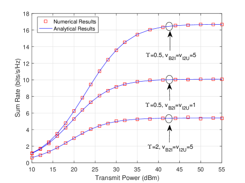
Fig. 3 shows the impact of IRS directions on the sum rate. For the “non-orthogonal IRS directions” case, the locations of 4 IRSs are given by (278,113,20),(338,41,20),(367,45,20)(278,113,-20),(338,41,-20),(367,-45,-20) and (370,151,20)(370,-151,-20), respectively. For the “orthogonal IRS directions” case, the locations of 4 IRSs are given by (240,178,20),(333,68,20),(362,75,20)(240,178,-20),(333,68,-20),(362,-75,-20) and (319,241,20)(319,-241,-20), respectively. The analytical curve with orthogonal IRS directions ( 𝐚B2I,mT𝐚B2I,i=0,mi{\bf a}_{\text{B2I},m}^{T}{\bf a}_{\text{B2I},i}^{*}=0,m\neq i ) is plotted according to Corollary 2, while the analytical curve with non-orthogonal IRS directions is obtained according to Theorem 2. We can see that the analytical results with orthogonal IRS directions well match their numerical results, which verifies our analytical results in Corollary 2. Moreover, as expected in Proposition 2 , the achievable sum rate with orthogonal IRS directions is much higher than that with non-orthogonal IRS directions, due to the decreased interference from multiple IRSs.

Refer to caption
Figure 3: The impact of IRS directions on the sum rate with Υ=1\Upsilon=1m.

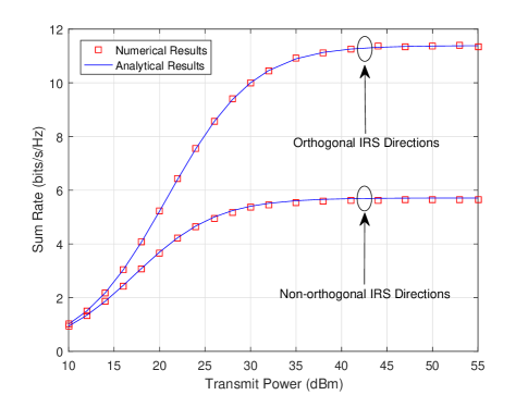
Fig. 4 shows the impact of the IRS location on the sum rate, when the locations of users are fixed. As can be readily observed, the sum rate is not a monotonic function with respect to the BS-IRS distances. The worst sum rate occurs when the IRSs are deployed in the middle of the BS and users, and the sum rate improves when moving the IRSs towards the BS or users, which indicates that it is desirable to deploy the IRSs near the BS or users.

Refer to caption
Figure 4: The impact of the IRS location on the sum rate.

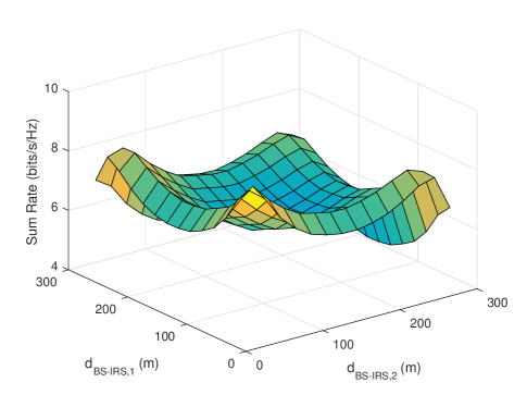
Fig. 5 shows the impact of the number of reflecting elements on the sum rate, where the approximate results are obtained according to Corollary 3. We can see that the approximate results matches the numerical results well, thereby validating the correctness of Corollary 3. Moreover, as expected in Corollary 3, the sum rate grows logarithmically with the number of reflecting elements, indicating the great benefit of applying a large number of reflecting elements. In addition, increasing the antenna number can also improve the sum rate due to the increased BS beam gain.

Refer to caption
Figure 5: The impact of the number of reflecting elements on the sum rate.

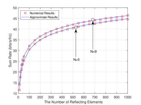
Fig. 6 shows the impact of the antenna number on the sum rate, where the “Limit” curve is generated according to Corollary 4. As expected, the sum rate increases with the number of antennas and gradually converges to a limit, which is mainly determined by the number of reflecting elements and the Rician K-factor of IRS-user channels. It can be seen that the sum rate limit increases with the number reflecting elements, while decreases as the the Rician K-factor of IRS-user channels becomes smaller due to more interference caused by NLOS paths.

Refer to caption
Figure 6: The impact of the number of BS antennas on the sum rate with perfect location information and ρd=40dBm\rho_{d}=40\text{dBm}.

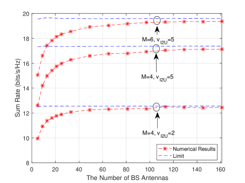
Fig. 7 illustrates the impact of the Rician K-factor on the sum rate, where the “Limit” curve is generated according to Corollary 5. It can be seen that the sum rate grows with the Rician K-factor and gradually converges to a limit, which is mainly determined by the number of reflecting elements. As expected in Corollary 5, increasing the number of reflecting elements greatly improves the sum rate, due to both the phase shift beamforming gain and the inherent aperture gain of the IRS. For instance, with a large Rician K-factor, the sum rate increases significantly from about 5 bits/s/Hz to about 11 bits/s/Hz, as the number of reflecting elements grows from 4 to 8.

Refer to caption
Figure 7: The impact of the Rician K-factor on the sum rate with perfect location information.

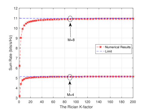
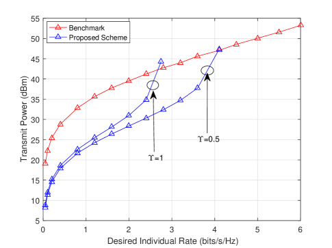
Fig. 8 shows the performance of the proposed beamforming scheme, where the optimal power control scheme discussed in Section VI is performed, and we assume R¯k=R¯,k=1,,K\bar{R}_{k}=\bar{R},k=1,...,K with R¯\bar{R} being the desired individual rate. For comparison, the joint optimization algorithm in [3] is presented as the benchmark, where the multiple IRSs are treated as a big distributed IRS. It can be observed that, when the desired rate is not very high, the proposed scheme is superior to the benchmark scheme. This is reasonable because with small rate constraint, the required transmit power is not high, as such, the system is likely to be noise-limited. In a noise-limited scenario, the MRC-based scheme is near optimal. Then, combining with the optimal power control algorithm eventually yields superior performance. However, as the rate constraint becomes stringent, the required transmit power grows and the system becomes interference-limited. Then, the performance of the proposed MRC scheme deteriorates significantly due to severe interference, and becomes inferior to the benchmark scheme. In addition, it may become infeasible if the desired rate is greater than a threshold. The reason is that the proposed beamforming scheme is designed without considering interference suppression, which is only partially addressed by power control and proper IRS configurations, i.e., deploying multiple IRSs at distinct directions, increasing the distance between different IRSs, and assigning each user to its nearest IRS. In contrast, the benchmark scheme assumes perfect CSI and adopts a joint optimization method, where the transmit beam and the phase shift beam are optimized by solving two semidefinite programming (SDP) sub-problems iteratively. Hence, the benchmark scheme can better deal with the inter-user interference.

Refer to caption
Figure 8: The performance of the proposed beamforming scheme .

VIII Conclusion

This paper has proposed a location information aided multi-IRS system. Based on the imperfect GPS location information, the effective angles are estimated, and the statistics of the angle estimation error are derived. Then, exploiting the estimated angles, low-complexity transmit beam and IRS phase shift beam have been designed, and closed-form expressions are derived for the achievable rate, which facilitates the characterization of the benefits of deploying a large number of BS antennas or reflecting elements. The findings suggest that the IRS-aided link can obtain a power gain of order NM2NM^{2}. With a large number of reflecting elements, the individual SINR is proportional to MM, while becomes proportional to M2M^{2} when there are no NLOS paths. Besides, it is demonstrated that the achievable rate degrades significantly as user location uncertainty increases. Furthermore, the analytical findings suggest that IRSs should be deployed at distinct directions and be far away from each other to reduce the interference from multiple IRSs. Finally, based on the proposed beamforming scheme, an optimal power control scheme is proposed to minimize the total transmit power under individual rate constraints. For future works, the robust beamforming in the presence of location uncertainty can be investigated, to guarantee the worse-case quality of service requirement [35, 36]. Besides, when the number of users is greater than the number of IRSs, how to schedule users in different resource blocks and how to pair the user with the IRS are worth studying.

Appendix A Proof of Proposition 1

The effective AOD from the mm-th IRS to the kk-th user is given by

ϑy-I2U,mk=yI,myU,kdI2U,mk.\displaystyle\vartheta_{\text{y-I2U},mk}=\frac{y_{\text{I},m}-y_{\text{U},k}}{d_{\text{I2U},mk}}. (90)

Using (13), the above equation can be rewritten as

ϑy-I2U,mk=d^I2U,mkdI2U,mkϑ^y-I2U,mkΔyU,kdI2U,mk,\displaystyle\vartheta_{\text{y-I2U},mk}=\frac{\hat{d}_{\text{I2U},mk}}{d_{\text{I2U},mk}}\hat{\vartheta}_{\text{y-I2U},mk}-\frac{\Delta y_{\text{U},k}}{d_{\text{I2U},mk}}, (91)

where dI2U,mk=(zI,mzU,k)2+(yI,myU,k)2+(xI,mxU,k)2d_{\text{I2U},mk}=\sqrt{(z_{\text{I},m}-z_{\text{U},k})^{2}+(y_{\text{I},m}-y_{\text{U},k})^{2}+(x_{\text{I},m}-x_{\text{U},k})^{2}} is the distance between the BS and the kk-th user, and ΔyU,k=yU,ky^U,k\Delta y_{\text{U},k}=y_{\text{U},k}-\hat{y}_{\text{U},k} is the location error along the yy axis.

Next, we focus on the term d^I2U,mkdI2U,mk\frac{\hat{d}_{\text{I2U},mk}}{d_{\text{I2U},mk}}:

d^I2U,mkdI2U,mk=(1+Q)12,\displaystyle\frac{\hat{d}_{\text{I2U},mk}}{d_{\text{I2U},mk}}={\left(1+Q\right)}^{-\frac{1}{2}}, (92)

where

Q\displaystyle Q ΔzU,k2+ΔyU,k2+ΔxU,k2d^I2U,mk22(ϑ^z-I2U,mkΔzU,k+ϑ^y-I2U,mkΔyU,k+ϑ^x-I2U,mkΔxU,kd^I2U,mk),\displaystyle\triangleq\frac{{\Delta z_{\text{U},k}}^{2}+{\Delta y_{\text{U},k}}^{2}+{\Delta x_{\text{U},k}}^{2}}{{\hat{d}}^{2}_{\text{I2U},mk}}-2\left(\frac{\hat{\vartheta}_{\text{z-I2U},mk}\Delta z_{\text{U},k}+\hat{\vartheta}_{\text{y-I2U},mk}\Delta y_{\text{U},k}+\hat{\vartheta}_{\text{x-I2U},mk}\Delta x_{\text{U},k}}{\hat{d}_{\text{I2U},mk}}\right), (93)
2(ϑ^z-I2U,mkΔzU,k+ϑ^y-I2U,mkΔyU,k+ϑ^x-I2U,mkΔxU,kd^I2U,mk),\displaystyle\approx-2\left(\frac{\hat{\vartheta}_{\text{z-I2U},mk}\Delta z_{\text{U},k}+\hat{\vartheta}_{\text{y-I2U},mk}\Delta y_{\text{U},k}+\hat{\vartheta}_{\text{x-I2U},mk}\Delta x_{\text{U},k}}{\hat{d}_{\text{I2U},mk}}\right),

where ϑ^x-I2U,mkxI,mx^U,kd^I2U,mk\hat{\vartheta}_{\text{x-I2U},mk}\triangleq\frac{x_{\text{I},m}-\hat{x}_{\text{U},k}}{\hat{d}_{\text{I2U},mk}}, ϑ^z-I2U,mkzI,mz^U,kd^I2U,mk\hat{\vartheta}_{\text{z-I2U},mk}\triangleq\frac{z_{\text{I},m}-\hat{z}_{\text{U},k}}{\hat{d}_{\text{I2U},mk}}, ΔzU,k=zU,kz^U,k\Delta z_{\text{U},k}=z_{\text{U},k}-\hat{z}_{\text{U},k} and ΔxU,k=xU,kx^U,k\Delta x_{\text{U},k}=x_{\text{U},k}-\hat{x}_{\text{U},k} are location errors along zz and xx axes, respectively.

Using the Taylor expansion of (1+Q)12{\left(1+Q\right)}^{-\frac{1}{2}} at Q=0Q=0, we have

d^I2U,mkdI2U,mk=112Q.\displaystyle\frac{\hat{d}_{\text{I2U},mk}}{d_{\text{I2U},mk}}=1-\frac{1}{2}Q. (94)

Substituting (94) into (91), we obtain

ϑy-I2U,mk=(112Q)ϑ^y-I2U,mk(112Q)ΔyU,kd^I2U,mkϑ^y-I2U,mk+ϵy-I2U,mk,\displaystyle\vartheta_{\text{y-I2U},mk}=\left(1-\frac{1}{2}Q\right)\hat{\vartheta}_{\text{y-I2U},mk}-\left(1-\frac{1}{2}Q\right)\frac{\Delta y_{\text{U},k}}{\hat{d}_{\text{I2U},mk}}\approx\hat{\vartheta}_{\text{y-I2U},mk}+\epsilon_{\text{y-I2U},mk}, (95)

where the estimation error of the effective AOD along yy axis, ϵy-I2U,mk\epsilon_{\text{y-I2U},mk}, is given by

ϵy-I2U,mk\displaystyle\epsilon_{\text{y-I2U},mk} =12Qϑ^y-I2U,mkΔyU,kd^I2U,mk,\displaystyle=-\frac{1}{2}Q\hat{\vartheta}_{\text{y-I2U},mk}-\frac{\Delta y_{\text{U},k}}{\hat{d}_{\text{I2U},mk}}, (96)
=(ϑ^y-I2U,mk21)ΔyU,k+ϑ^y-I2U,mkϑ^z-I2U,mkΔzU,k+ϑ^y-I2U,mkϑ^x-I2U,mkΔxU,kd^I2U,mk.\displaystyle=\frac{\left(\hat{\vartheta}^{2}_{\text{y-I2U},mk}-1\right)\Delta y_{\text{U},k}+\hat{\vartheta}_{\text{y-I2U},mk}\hat{\vartheta}_{\text{z-I2U},mk}\Delta z_{\text{U},k}+\hat{\vartheta}_{\text{y-I2U},mk}\hat{\vartheta}_{\text{x-I2U},mk}\Delta x_{\text{U},k}}{\hat{d}_{\text{I2U},mk}}.

To this end, we complete the proof of (14).

Appendix B Proof of Theorem 1

The equation (14) given by Proposition 1 can be rewritten as

ϵy-I2U,mk=ay-I2U,mkΔyU,k+by-I2U,mkΔzU,k+cy-I2U,mkΔxU,k\displaystyle\epsilon_{\text{y-I2U},mk}=a_{\text{y-I2U},mk}\Delta y_{\text{U},k}+b_{\text{y-I2U},mk}\Delta z_{\text{U},k}+c_{\text{y-I2U},mk}\Delta x_{\text{U},k} (97)

where ay-I2U,mkϑ^y-I2U,mk21d^I2U,mka_{\text{y-I2U},mk}\triangleq\frac{\hat{\vartheta}^{2}_{\text{y-I2U},mk}-1}{\hat{d}_{\text{I2U},mk}}, by-I2U,mkϑ^y-I2U,mkϑ^z-I2U,mkd^I2U,mkb_{\text{y-I2U},mk}\triangleq\frac{\hat{\vartheta}_{\text{y-I2U},mk}\hat{\vartheta}_{\text{z-I2U},mk}}{\hat{d}_{\text{I2U},mk}}, and cy-I2U,mkϑ^y-I2U,mkϑ^x-I2U,mkd^I2U,mkc_{\text{y-I2U},mk}\triangleq\frac{\hat{\vartheta}_{\text{y-I2U},mk}\hat{\vartheta}_{\text{x-I2U},mk}}{\hat{d}_{\text{I2U},mk}}.

The cumulative distribution function (CDF) of ϵy-I2U,mk\epsilon_{\text{y-I2U},mk} is given by

Fϵy-I2U,mk(x)\displaystyle F_{\epsilon_{\text{y-I2U},mk}}\left(x\right) =P(ϵy-I2U,mk<x)\displaystyle=P\left(\epsilon_{\text{y-I2U},mk}<x\right) (98)
=P(ay-I2U,mkΔyU,k+by-I2U,mkΔzU,k+cy-I2U,mkΔxU,kx<0).\displaystyle=P\left(a_{\text{y-I2U},mk}\Delta y_{\text{U},k}+b_{\text{y-I2U},mk}\Delta z_{\text{U},k}+c_{\text{y-I2U},mk}\Delta x_{\text{U},k}-x<0\right).

Recall that the point (ΔxU,k,ΔyU,k,ΔzU,k)(\Delta x_{\text{U},k},\Delta y_{\text{U},k},\Delta z_{\text{U},k}) is uniformly distributed within a sphere with the radius Υ\Upsilon and the origin (0,0,0)(0,0,0). The distance from the origin (0,0,0)(0,0,0) to the plane ay-I2U,mkΔyU,k+by-I2U,mkΔzU,k+cy-I2U,mkΔxU,kx=0a_{\text{y-I2U},mk}\Delta y_{\text{U},k}+b_{\text{y-I2U},mk}\Delta z_{\text{U},k}+c_{\text{y-I2U},mk}\Delta x_{\text{U},k}-x=0 is

d=|x|ay-I2U,mk2+by-I2U,mk2+cy-I2U,mk2.\displaystyle d=\frac{\left|x\right|}{\sqrt{a^{2}_{\text{y-I2U},mk}+b^{2}_{\text{y-I2U},mk}+c^{2}_{\text{y-I2U},mk}}}. (99)

For Υay-I2U,mk2+by-I2U,mk2+cy-I2U,mk2x0-\Upsilon\sqrt{a^{2}_{\text{y-I2U},mk}+b^{2}_{\text{y-I2U},mk}+c^{2}_{\text{y-I2U},mk}}\leq x\leq 0, we have

Fϵy-I2U,mk(x)=1/(4πΥ33)dΥπ(Υ2t2)𝑑t\displaystyle F_{\epsilon_{\text{y-I2U},mk}}\left(x\right)=1/\left(\frac{4\pi\Upsilon^{3}}{3}\right)\int_{d}^{\Upsilon}\pi\left(\Upsilon^{2}-t^{2}\right)dt (100)
=1/(4πΥ33)(π3d3πΥ2d+2π3Υ3).\displaystyle=1/\left(\frac{4\pi\Upsilon^{3}}{3}\right)\left(\frac{\pi}{3}d^{3}-\pi\Upsilon^{2}d+\frac{2\pi}{3}\Upsilon^{3}\right).

For 0<xΥay-I2U,mk2+by-I2U,mk2+cy-I2U,mk20<x\leq\Upsilon\sqrt{a^{2}_{\text{y-I2U},mk}+b^{2}_{\text{y-I2U},mk}+c^{2}_{\text{y-I2U},mk}}, we have

Fϵy-I2U,mk(x)=11/(4πΥ33)dΥπ(Υ2t2)𝑑t\displaystyle F_{\epsilon_{\text{y-I2U},mk}}\left(x\right)=1-1/\left(\frac{4\pi\Upsilon^{3}}{3}\right)\int_{d}^{\Upsilon}\pi\left(\Upsilon^{2}-t^{2}\right)dt (101)
=11/(4πΥ33)(π3d3πΥ2d+2π3Υ3).\displaystyle=1-1/\left(\frac{4\pi\Upsilon^{3}}{3}\right)\left(\frac{\pi}{3}d^{3}-\pi\Upsilon^{2}d+\frac{2\pi}{3}\Upsilon^{3}\right).

Substituting (99) into (100) and (101), we obtain

Fϵy-I2U,mk(x)\displaystyle F_{\epsilon_{\text{y-I2U},mk}}\left(x\right) =1214Υ3(ay-I2U,mk2+by-I2U,mk2+cy-I2U,mk2)3/2x3\displaystyle=\frac{1}{2}-\frac{1}{4\Upsilon^{3}}{\left(a^{2}_{\text{y-I2U},mk}+b^{2}_{\text{y-I2U},mk}+c^{2}_{\text{y-I2U},mk}\right)}^{-3/2}x^{3} (102)
+34Υ(ay-I2U,mk2+by-I2U,mk2+cy-I2U,mk2)1/2x,\displaystyle+\frac{3}{4\Upsilon}{\left(a^{2}_{\text{y-I2U},mk}+b^{2}_{\text{y-I2U},mk}+c^{2}_{\text{y-I2U},mk}\right)}^{-1/2}x,

for |x|Υay-I2U,mk2+by-I2U,mk2+cy-I2U,mk2\left|x\right|\leq\Upsilon\sqrt{a^{2}_{\text{y-I2U},mk}+b^{2}_{\text{y-I2U},mk}+c^{2}_{\text{y-I2U},mk}}.

Define Φy-I2U,mk(ϑ^y-I2U,mk21)2+ϑ^y-I2U,mk2ϑ^z-I2U,mk2+ϑ^y-I2U,mk2ϑ^x-I2U,mk2\Phi_{\text{y-I2U},mk}\triangleq\sqrt{{\left(\hat{\vartheta}^{2}_{\text{y-I2U},mk}-1\right)}^{2}+\hat{\vartheta}^{2}_{\text{y-I2U},mk}\hat{\vartheta}^{2}_{\text{z-I2U},mk}+\hat{\vartheta}^{2}_{\text{y-I2U},mk}\hat{\vartheta}^{2}_{\text{x-I2U},mk}}. The corresponding PDF is given by

fϵy-I2U,mk(x)=Fϵy-I2U,mk(x)x=3d^I2U,mk34Υ3Φy-I2U,mk3x2+3d^I2U,mk4ΥΦy-I2U,mk1,\displaystyle f_{\epsilon_{\text{y-I2U},mk}}\left(x\right)=\frac{\partial F_{\epsilon_{\text{y-I2U},mk}}\left(x\right)}{\partial x}=-\frac{3{\hat{d}}^{3}_{\text{I2U},mk}}{4\Upsilon^{3}}{\Phi}^{-3}_{\text{y-I2U},mk}x^{2}+\frac{3{\hat{d}}_{\text{I2U},mk}}{4\Upsilon}{\Phi}^{-1}_{\text{y-I2U},mk},

for |x|Υd^I2U,mkΦy-I2U,mk|x|\leq\frac{\Upsilon}{\hat{d}_{\text{I2U},mk}}{\Phi}_{\text{y-I2U},mk}.

Based on the above PDF, the mean and the variance of ϵy-I2U,mk\epsilon_{\text{y-I2U},mk} can be obtained.

Appendix C Proof of Lemma 1

Denote ϵk,mn,sl(s1)ϵy-I2U,mk(l1)ϵy-I2U,nk\epsilon_{k,mn,sl}\triangleq\left(s-1\right)\epsilon_{\text{y-I2U},mk}-\left(l-1\right)\epsilon_{\text{y-I2U},nk}.

ζy-I2U,k,mn,sl𝔼{ϱI2U,mk,sϱI2U,nk,l}=𝔼{ejπϵk,mn,sl}.\displaystyle\zeta_{\text{y-I2U},k,mn,sl}\triangleq\mathbb{E}\left\{\varrho_{\text{I2U},mk,s}\varrho_{\text{I2U},nk,l}^{*}\right\}=\mathbb{E}\left\{e^{j\pi\epsilon_{k,mn,sl}}\right\}. (103)

We can rewrite ϵk,mn,sl\epsilon_{k,mn,sl} as

ϵk,mn,sl=ak,mn,slΔyU,k+bk,mn,slΔzU,k+ck,mn,slΔxU,k,\displaystyle\epsilon_{k,mn,sl}=a_{k,mn,sl}\Delta y_{\text{U},k}+b_{k,mn,sl}\Delta z_{\text{U},k}+c_{k,mn,sl}\Delta x_{\text{U},k}, (104)

where

ak,mn,sl(s1)ϑ^y-I2U,mk21d^I2U,mk(l1)ϑ^y-I2U,nk21d^I2U,nk,\displaystyle a_{k,mn,sl}\triangleq\left(s-1\right)\frac{\hat{\vartheta}^{2}_{\text{y-I2U},mk}-1}{\hat{d}_{\text{I2U},mk}}-\left(l-1\right)\frac{\hat{\vartheta}^{2}_{\text{y-I2U},nk}-1}{\hat{d}_{\text{I2U},nk}}, (105)
bk,mn,sl(s1)ϑ^y-I2U,mkϑ^z-I2U,mkd^I2U,mk(l1)ϑ^y-I2U,nkϑ^z-I2U,nkd^I2U,nk,\displaystyle b_{k,mn,sl}\triangleq\left(s-1\right)\frac{\hat{\vartheta}_{\text{y-I2U},mk}\hat{\vartheta}_{\text{z-I2U},mk}}{\hat{d}_{\text{I2U},mk}}-\left(l-1\right)\frac{\hat{\vartheta}_{\text{y-I2U},nk}\hat{\vartheta}_{\text{z-I2U},nk}}{\hat{d}_{\text{I2U},nk}}, (106)
ck,mn,sl(s1)ϑ^y-I2U,mkϑ^x-I2U,mkd^I2U,mk(l1)ϑ^y-I2U,nkϑ^x-I2U,nkd^I2U,nk.\displaystyle c_{k,mn,sl}\triangleq\left(s-1\right)\frac{\hat{\vartheta}_{\text{y-I2U},mk}\hat{\vartheta}_{\text{x-I2U},mk}}{\hat{d}_{\text{I2U},mk}}-\left(l-1\right)\frac{\hat{\vartheta}_{\text{y-I2U},nk}\hat{\vartheta}_{\text{x-I2U},nk}}{\hat{d}_{\text{I2U},nk}}. (107)

Following the similar process of the proof of Theorem 1, we have the PDF of ϵk,mn,sl\epsilon_{k,mn,sl} given by

fϵk,mn,sl(x)\displaystyle f_{\epsilon_{k,mn,sl}}\left(x\right) (108)
=34Υ3(ak,mn,sl2+bk,mn,sl2+ck,mn,sl2)3/2x2+34Υ(ak,mn,sl2+bk,mn,sl2+ck,mn,sl2)1/2\displaystyle=-\frac{3}{4\Upsilon^{3}}{\left(a^{2}_{k,mn,sl}+b^{2}_{k,mn,sl}+c^{2}_{k,mn,sl}\right)}^{-3/2}x^{2}+\frac{3}{4\Upsilon}{\left(a^{2}_{k,mn,sl}+b^{2}_{k,mn,sl}+c^{2}_{k,mn,sl}\right)}^{-1/2}
=34Υ3Φk,mn,sl3x2+34ΥΦk,mn,sl,\displaystyle=-\frac{3}{4\Upsilon^{3}\Phi_{k,mn,sl}^{3}}x^{2}+\frac{3}{4\Upsilon\Phi_{k,mn,sl}},

for |x|ΥΦk,mn,sl|x|\leq\Upsilon{\Phi}_{k,mn,sl}, where we define

Φk,mn,slak,mn,sl2+bk,mn,sl2+ck,mn,sl2.\displaystyle\Phi_{k,mn,sl}\triangleq\sqrt{a^{2}_{k,mn,sl}+b^{2}_{k,mn,sl}+c^{2}_{k,mn,sl}}. (109)

According to the above PDF, the expectation ζy-I2U,k,mn,sl=𝔼{ejπϵk,mn,sl}\zeta_{\text{y-I2U},k,mn,sl}=\mathbb{E}\left\{e^{j\pi\epsilon_{k,mn,sl}}\right\} can be calculated as

ζk,mn,sl=𝔼{ejπϵk,mn,sl}\displaystyle\zeta_{k,mn,sl}=\mathbb{E}\left\{e^{j\pi\epsilon_{k,mn,sl}}\right\} (110)
={1,s=1andl=13ϖk,mn,sl2(sinϖk,mn,slϖk,mn,slcosϖk,mn,sl),else\displaystyle=\begin{cases}1,&s=1\ \text{and}\ l=1\\ \frac{3}{\varpi_{k,mn,sl}^{2}}\left(\frac{\sin\varpi_{k,mn,sl}}{\varpi_{k,mn,sl}}-\cos\varpi_{k,mn,sl}\right),&\text{else}\end{cases}

where ϖk,mn,slπΦk,mn,slΥ\varpi_{k,mn,sl}\triangleq{\pi{\Phi}_{k,mn,sl}\Upsilon}.

Appendix D Proof of Theorem 2

D-A Calculate AkA_{k}

Recall that 𝐰k=ηkρdN𝐚B2I,k{\bf w}_{k}=\sqrt{\frac{\eta_{k}\rho_{d}}{N}}{\bf a}_{\text{B2I},k}^{*}. We have

𝔼{𝐠kT𝐰k}=ηiρdN𝔼{𝐠kT𝐚B2I,k}\displaystyle\mathbb{E}\left\{{\bf g}_{k}^{T}{\bf w}_{k}\right\}=\sqrt{\frac{\eta_{i}\rho_{d}}{N}}\mathbb{E}\left\{{\bf g}_{k}^{T}{\bf a}_{\text{B2I},k}^{*}\right\} (111)
=ηkρdN𝔼{𝐠I2U,kkT𝚯k𝐆B2I,k𝐚B2I,k}+ηkρdNmkK𝔼{𝐠I2U,mkT𝚯m𝐆B2I,m𝐚B2I,k}.\displaystyle=\sqrt{\frac{\eta_{k}\rho_{d}}{N}}\mathbb{E}\left\{{\bf g}_{\text{I2U},kk}^{T}{\mbox{\boldmath$\Theta$}_{k}}{\bf G}_{\text{B2I},k}{\bf a}_{\text{B2I},k}^{*}\right\}+\sqrt{\frac{\eta_{k}\rho_{d}}{N}}\sum\limits_{m\neq k}^{K}\mathbb{E}\left\{{\bf g}_{\text{I2U},mk}^{T}{\mbox{\boldmath$\Theta$}_{m}}{\bf G}_{\text{B2I},m}{\bf a}_{\text{B2I},k}^{*}\right\}.

We first calculate 𝔼{𝐠I2U,mkT𝚯m𝐆B2I,m𝐚B2I,k},mk\mathbb{E}\left\{{\bf g}_{\text{I2U},mk}^{T}{\mbox{\boldmath$\Theta$}_{m}}{\bf G}_{\text{B2I},m}{\bf a}_{\text{B2I},k}^{*}\right\},m\neq k:

𝔼{𝐠I2U,mkT𝚯m𝐆B2I,m𝐚B2I,k}=βB2I2U,mk𝔼{𝐠¯I2U,mkT𝚯m𝐛B2I,m}𝐚B2I,mT𝐚B2I,k\displaystyle\mathbb{E}\left\{{\bf g}_{\text{I2U},mk}^{T}{\mbox{\boldmath$\Theta$}_{m}}{\bf G}_{\text{B2I},m}{\bf a}_{\text{B2I},k}^{*}\right\}=\sqrt{\beta_{\text{B2I2U},mk}}\mathbb{E}\left\{\bar{\bf g}_{\text{I2U},mk}^{T}{\mbox{\boldmath$\Theta$}_{m}}{\bf b}_{\text{B2I},m}\right\}{\bf a}^{T}_{\text{B2I},m}{\bf a}_{\text{B2I},k}^{*} (112)
=𝐚B2I,mT𝐚B2I,kβB2I2U,mk𝔼{𝝃mT(𝐠¯I2U,mk𝐛B2I,m)}\displaystyle={\bf a}^{T}_{\text{B2I},m}{\bf a}_{\text{B2I},k}^{*}\sqrt{\beta_{\text{B2I2U},mk}}\mathbb{E}\left\{{\mbox{\boldmath$\xi$}}^{T}_{m}\left(\bar{\bf g}_{\text{I2U},mk}\odot{\bf b}_{\text{B2I},m}\right)\right\}
=𝐚B2I,mT𝐚B2I,kβB2I2U,mks=1M𝔼{ϱI2U,mk,s}[𝐠¯^I2U,mk]s[𝐠¯^I2U,mm]s.\displaystyle={\bf a}^{T}_{\text{B2I},m}{\bf a}_{\text{B2I},k}^{*}\sqrt{\beta_{\text{B2I2U},mk}}\sum\limits_{s=1}^{M}\mathbb{E}\left\{\varrho_{\text{I2U},mk,s}\right\}{\left[{\hat{\bar{\bf g}}}_{\text{I2U},mk}\right]}_{s}{\left[{\hat{\bar{\bf g}}}_{\text{I2U},mm}\right]}_{s}^{*}.

Denoting ζy-I2U,mk,s𝔼{ϱI2U,mk,s}\zeta_{\text{y-I2U},mk,s}\triangleq\mathbb{E}\left\{\varrho_{\text{I2U},mk,s}\right\} and using the results given by Theorem 1, we have

ζy-I2U,mk,s\displaystyle\zeta_{\text{y-I2U},mk,s} =ΥΦy-I2U,mkd^I2U,mkΥΦy-I2U,mkd^I2U,mk(3d^I2U,mk34Υ3Φy-I2U,mk3x2+3d^I2U,mk4ΥΦy-I2U,mk1)ejπ(s1)x𝑑x\displaystyle=\int_{-\frac{\Upsilon{\Phi}_{\text{y-I2U},mk}}{\hat{d}_{\text{I2U},mk}}}^{\frac{\Upsilon{\Phi}_{\text{y-I2U},mk}}{\hat{d}_{\text{I2U},mk}}}\left(-\frac{3{\hat{d}}^{3}_{\text{I2U},mk}}{4\Upsilon^{3}}{\Phi}^{-3}_{\text{y-I2U},mk}x^{2}+\frac{3{\hat{d}}_{\text{I2U},mk}}{4\Upsilon}{\Phi}^{-1}_{\text{y-I2U},mk}\right)e^{j\pi\left(s-1\right)x}\ dx (113)
={3ϖy-I2U,mk,s2(sinϖy-I2U,mk,sϖy-I2U,mk,scosϖy-I2U,mk,s)s11s=1.\displaystyle=\begin{cases}\frac{3}{\varpi_{\text{y-I2U},mk,s}^{2}}\left(\frac{\sin\varpi_{\text{y-I2U},mk,s}}{\varpi_{\text{y-I2U},mk,s}}-\cos\varpi_{\text{y-I2U},mk,s}\right)&s\!\neq\!1\\ 1&s\!=\!1\end{cases}.

Thus, we obtain

𝔼{𝐠I2U,mkT𝚯m𝐆B2I,m𝐚B2I,k}\displaystyle\mathbb{E}\left\{{\bf g}_{\text{I2U},mk}^{T}{\mbox{\boldmath$\Theta$}_{m}}{\bf G}_{\text{B2I},m}{\bf a}_{\text{B2I},k}^{*}\right\} (114)
=𝐚B2I,mT𝐚B2I,kβB2I2U,mks=1Mζy-I2U,mk,s[𝐠¯^I2U,mk]s[𝐠¯^I2U,mm]s.\displaystyle={\bf a}^{T}_{\text{B2I},m}{\bf a}_{\text{B2I},k}^{*}\sqrt{\beta_{\text{B2I2U},mk}}\sum\limits_{s=1}^{M}\zeta_{\text{y-I2U},mk,s}{\left[{\hat{\bar{\bf g}}}_{\text{I2U},mk}\right]}_{s}{\left[{\hat{\bar{\bf g}}}_{\text{I2U},mm}\right]}_{s}^{*}.

Then, we start the calculation of the first term:

𝔼{𝐠I2U,kkT𝚯k𝐆B2I,k𝐚B2I,k}=NβB2I2U,kk𝔼{𝐠¯I2U,kkT𝚯k𝐛B2I,k}\displaystyle\mathbb{E}\left\{{\bf g}_{\text{I2U},kk}^{T}{\mbox{\boldmath$\Theta$}_{k}}{\bf G}_{\text{B2I},k}{\bf a}_{\text{B2I},k}^{*}\right\}=N\sqrt{\beta_{\text{B2I2U},kk}}\mathbb{E}\left\{\bar{\bf g}_{\text{I2U},kk}^{T}{\mbox{\boldmath$\Theta$}_{k}}{\bf b}_{\text{B2I},k}\right\} (115)
=NβB2I2U,kk𝔼{𝝃T(𝐠¯I2U,kk𝐛B2I,k)},\displaystyle=N\sqrt{\beta_{\text{B2I2U},kk}}\mathbb{E}\left\{{\mbox{\boldmath$\xi$}}^{T}\left(\bar{\bf g}_{\text{I2U},kk}\odot{\bf b}_{\text{B2I},k}\right)\right\},

where βB2I2U,mkαB2I,mvB2I,mαI2U,mkvI2U,mk(vB2I,m+1)(vI2U,mk+1)\beta_{\text{B2I2U},mk}\triangleq\frac{\alpha_{\text{B2I},m}v_{\text{B2I},m}\alpha_{\text{I2U},mk}v_{\text{I2U},mk}}{(v_{\text{B2I},m}+1)(v_{\text{I2U},mk}+1)}.

Recall that 𝝃k=(𝐠¯^I2U,kk𝐛B2I,k){\mbox{\boldmath$\xi$}}_{k}=\left({\hat{\bar{\bf g}}}_{\text{I2U},kk}\odot{\bf b}_{\text{B2I},k}\right)^{*}. The above equation can be expressed as

𝔼{𝐠I2U,kkT𝚯k𝐆B2I,k𝐚B2I,k}=NβB2I2U,kks=1M𝔼{ϱI2U,kk,s}.\displaystyle\mathbb{E}\left\{{\bf g}_{\text{I2U},kk}^{T}{\mbox{\boldmath$\Theta$}_{k}}{\bf G}_{\text{B2I},k}{\bf a}_{\text{B2I},k}^{*}\right\}=N\sqrt{\beta_{\text{B2I2U},kk}}\sum\limits_{s=1}^{M}\mathbb{E}\left\{\varrho_{\text{I2U},kk,s}\right\}. (116)

As such, we obtain

𝔼{𝐠I2U,kkT𝚯k𝐆B2I,k𝐚B2I,k}=NβB2I2U,kks=1Mζy-I2U,kk,s.\displaystyle\mathbb{E}\left\{{\bf g}_{\text{I2U},kk}^{T}{\mbox{\boldmath$\Theta$}_{k}}{\bf G}_{\text{B2I},k}{\bf a}_{\text{B2I},k}^{*}\right\}=N\sqrt{\beta_{\text{B2I2U},kk}}\sum\limits_{s=1}^{M}\zeta_{\text{y-I2U},kk,s}. (117)

Combining 114 and 117 yields

Ak=ηkρdN|m=1Ks=1MβB2I2U,mk𝐚B2I,mT𝐚B2I,kζy-I2U,mk,s[𝐠¯^I2U,mk]s[𝐠¯^I2U,mm]s|2.\displaystyle A_{k}=\frac{\eta_{k}\rho_{d}}{N}\left|\sum\limits_{m=1}^{K}\sum\limits_{s=1}^{M}\sqrt{\beta_{\text{B2I2U},mk}}{\bf a}^{T}_{\text{B2I},m}{\bf a}_{\text{B2I},k}^{*}\zeta_{\text{y-I2U},mk,s}{\left[{\hat{\bar{\bf g}}}_{\text{I2U},mk}\right]}_{s}{\left[{\hat{\bar{\bf g}}}_{\text{I2U},mm}\right]}_{s}^{*}\right|^{2}. (118)

D-B Calculate Ck,iC_{k,i}

We can rewrite Ck,iC_{k,i} as

Ck,i\displaystyle C_{k,i} =𝔼{|𝐠kT𝐰i|2}=ηiρdNm=1Kn=1K𝔼{𝐠I2U,mkT𝚯m𝐆B2I,m𝐚B2I,i𝐚B2I,iT𝐆B2I,nH𝚯nH𝐠I2U,nk}.\displaystyle=\mathbb{E}\left\{{\left|{{\bf g}_{k}^{T}{\bf w}_{i}}\right|}^{2}\right\}=\frac{\eta_{i}\rho_{d}}{N}\sum\limits_{m=1}^{K}\sum\limits_{n=1}^{K}\mathbb{E}\left\{{\bf g}_{\text{I2U},mk}^{T}{\mbox{\boldmath$\Theta$}_{m}}{\bf G}_{\text{B2I},m}{\bf a}_{\text{B2I},i}^{*}{\bf a}_{\text{B2I},i}^{T}{\bf G}_{\text{B2I},n}^{H}{\mbox{\boldmath$\Theta$}_{n}}^{H}{\bf g}_{\text{I2U},nk}^{*}\right\}. (119)

1) For m=nm=n, we have

𝔼{𝐠I2U,mkT𝚯m𝐆B2I,m𝐚B2I,i𝐚B2I,iT𝐆B2I,nH𝚯nH𝐠I2U,nk}\displaystyle\mathbb{E}\left\{{\bf g}_{\text{I2U},mk}^{T}{\mbox{\boldmath$\Theta$}_{m}}{\bf G}_{\text{B2I},m}{\bf a}_{\text{B2I},i}^{*}{\bf a}_{\text{B2I},i}^{T}{\bf G}_{\text{B2I},n}^{H}{\mbox{\boldmath$\Theta$}_{n}}^{H}{\bf g}_{\text{I2U},nk}^{*}\right\} (120)
=𝔼{|𝐠I2U,mkT𝚯m𝐆B2I,m𝐚B2I,i|2}\displaystyle=\mathbb{E}\left\{\left|{\bf g}_{\text{I2U},mk}^{T}{\mbox{\boldmath$\Theta$}_{m}}{\bf G}_{\text{B2I},m}{\bf a}_{\text{B2I},i}\right|^{2}\right\}
=MβB2I2U,mkvI2U,mk|𝐚B2I,mT𝐚B2I,i|2+MNβB2I2U,mkvB2I,mvI2U,mk+MNβB2I2U,mkvB2I,m\displaystyle=M\frac{\beta_{\text{B2I2U},mk}}{v_{\text{I2U},mk}}\left|{\bf a}^{T}_{\text{B2I},m}{\bf a}_{\text{B2I},i}^{*}\right|^{2}+MN\frac{\beta_{\text{B2I2U},mk}}{v_{\text{B2I},m}v_{\text{I2U},mk}}+MN\frac{\beta_{\text{B2I2U},mk}}{v_{\text{B2I},m}}
+βB2I2U,mk𝔼{|𝐠¯I2U,mkT𝚯m𝐆¯B2I,m𝐚B2I,i|2}.\displaystyle+\beta_{\text{B2I2U},mk}\mathbb{E}\left\{\left|\bar{\bf g}_{\text{I2U},mk}^{T}{\mbox{\boldmath$\Theta$}_{m}}\bar{\bf G}_{\text{B2I},m}{\bf a}_{\text{B2I},i}^{*}\right|^{2}\right\}.

Next, we focus on the calculation of 𝔼{|𝐠¯I2U,mkT𝚯m𝐆¯B2I,m𝐚B2I,i|2}\mathbb{E}\left\{\left|\bar{\bf g}_{\text{I2U},mk}^{T}{\mbox{\boldmath$\Theta$}_{m}}\bar{\bf G}_{\text{B2I},m}{\bf a}_{\text{B2I},i}^{*}\right|^{2}\right\}.

𝔼{|𝐠¯I2U,mkT𝚯m𝐆¯B2I,m𝐚B2I,i|2}\displaystyle\mathbb{E}\left\{\left|\bar{\bf g}_{\text{I2U},mk}^{T}{\mbox{\boldmath$\Theta$}_{m}}\bar{\bf G}_{\text{B2I},m}{\bf a}_{\text{B2I},i}^{*}\right|^{2}\right\} (121)
=|𝐚B2I,mT𝐚B2I,i|2s=1Ml=1M𝔼{ϱI2U,mk,sl}[𝐠¯^I2U,mk]s[𝐠¯^I2U,mm]s[𝐠¯^I2U,mk]l[𝐠¯^I2U,mm]l,\displaystyle=\left|{\bf a}^{T}_{\text{B2I},m}{\bf a}_{\text{B2I},i}^{*}\right|^{2}\sum\limits_{s=1}^{M}\sum\limits_{l=1}^{M}\mathbb{E}\left\{\varrho_{\text{I2U},mk,sl}\right\}{\left[{\hat{\bar{\bf g}}}_{\text{I2U},mk}\right]}_{s}{\left[{\hat{\bar{\bf g}}}_{\text{I2U},mm}\right]}_{s}^{*}{\left[{\hat{\bar{\bf g}}}_{\text{I2U},mk}\right]}_{l}^{*}{\left[{\hat{\bar{\bf g}}}_{\text{I2U},mm}\right]}_{l},

where ϱI2U,mk,slejπ(sl)ϵy-I2U,mk\varrho_{\text{I2U},mk,sl}\triangleq e^{j\pi\left(s-l\right)\epsilon_{\text{y-I2U},mk}}.

Following the similar process of the calculation of 𝔼{ϱI2U,mk,s}\mathbb{E}\left\{\varrho_{\text{I2U},mk,s}\right\}, we have

ζy-I2U,mk,sl𝔼{ϱI2U,mk,sl}={3ϖy-I2U,mk,sl2(sinϖy-I2U,mk,slϖy-I2U,mk,slcosϖy-I2U,mk,sl)sl1s=l.\displaystyle\zeta_{\text{y-I2U},mk,sl}\triangleq\mathbb{E}\left\{\varrho_{\text{I2U},mk,sl}\right\}=\begin{cases}\frac{3}{\varpi_{\text{y-I2U},mk,sl}^{2}}\left(\frac{\sin\varpi_{\text{y-I2U},mk,sl}}{\varpi_{\text{y-I2U},mk,sl}}-\cos\varpi_{\text{y-I2U},mk,sl}\right)&s\!\neq\!l\\ 1&s\!=\!l\end{cases}. (122)

Thus, we obtain

𝔼{|𝐠¯I2U,mkT𝚯m𝐆¯B2I,m𝐚B2I,i|2}\displaystyle\mathbb{E}\left\{\left|\bar{\bf g}_{\text{I2U},mk}^{T}{\mbox{\boldmath$\Theta$}_{m}}\bar{\bf G}_{\text{B2I},m}{\bf a}_{\text{B2I},i}^{*}\right|^{2}\right\} (123)
=|𝐚B2I,mT𝐚B2I,i|2s=1Ml=1Mζy-I2U,mk,sl[𝐠¯^I2U,mk]s[𝐠¯^I2U,mm]s[𝐠¯^I2U,mk]l[𝐠¯^I2U,mm]l.\displaystyle=\left|{\bf a}^{T}_{\text{B2I},m}{\bf a}_{\text{B2I},i}^{*}\right|^{2}\sum\limits_{s=1}^{M}\sum\limits_{l=1}^{M}\zeta_{\text{y-I2U},mk,sl}{\left[{\hat{\bar{\bf g}}}_{\text{I2U},mk}\right]}_{s}{\left[{\hat{\bar{\bf g}}}_{\text{I2U},mm}\right]}_{s}^{*}{\left[{\hat{\bar{\bf g}}}_{\text{I2U},mk}\right]}_{l}^{*}{\left[{\hat{\bar{\bf g}}}_{\text{I2U},mm}\right]}_{l}.

2) For mnm\neq n, we have

𝔼{𝐠I2U,mkT𝚯m𝐆B2I,m𝐚B2I,i𝐚B2I,iT𝐆B2I,nH𝚯nH𝐠I2U,nk}\displaystyle\mathbb{E}\left\{{\bf g}_{\text{I2U},mk}^{T}{\mbox{\boldmath$\Theta$}_{m}}{\bf G}_{\text{B2I},m}{\bf a}_{\text{B2I},i}^{*}{\bf a}_{\text{B2I},i}^{T}{\bf G}_{\text{B2I},n}^{H}{\mbox{\boldmath$\Theta$}_{n}}^{H}{\bf g}_{\text{I2U},nk}^{*}\right\} (124)
=𝐚B2I,mT𝐚B2I,iβB2I2U,mk𝐚B2I,nH𝐚B2I,iβB2I2U,nk\displaystyle={\bf a}^{T}_{\text{B2I},m}{\bf a}_{\text{B2I},i}^{*}\sqrt{\beta_{\text{B2I2U},mk}}{\bf a}^{H}_{\text{B2I},n}{\bf a}_{\text{B2I},i}\sqrt{\beta_{\text{B2I2U},nk}}
×s=1Ml=1M𝔼{ϱI2U,mk,sϱI2U,nk,l}[𝐠¯^I2U,mk]s[𝐠¯^I2U,mm]s[𝐠¯^I2U,nk]l[𝐠¯^I2U,nn]l,\displaystyle\times\sum\limits_{s=1}^{M}\sum\limits_{l=1}^{M}\mathbb{E}\left\{\varrho_{\text{I2U},mk,s}\varrho_{\text{I2U},nk,l}^{*}\right\}{\left[{\hat{\bar{\bf g}}}_{\text{I2U},mk}\right]}_{s}{\left[{\hat{\bar{\bf g}}}_{\text{I2U},mm}\right]}_{s}^{*}{\left[{\hat{\bar{\bf g}}}_{\text{I2U},nk}\right]}_{l}^{*}{\left[{\hat{\bar{\bf g}}}_{\text{I2U},nn}\right]}_{l},

where 𝔼{ϱI2U,mk,sϱI2U,nk,l}=ζy-I2U,mk,nk,sl\mathbb{E}\left\{\varrho_{\text{I2U},mk,s}\varrho_{\text{I2U},nk,l}^{*}\right\}=\zeta_{\text{y-I2U},mk,nk,sl} given by Lemma 1.

Combining 1) and 2) yields

Ck,i=ηiρdNm=1K(MβB2I2U,mkvI2U,mk|𝐚B2I,mT𝐚B2I,i|2+MNβB2I2U,mkvB2I,mvI2U,mk++MNβB2I2U,mkvB2I,m)\displaystyle C_{k,i}=\frac{\eta_{i}\rho_{d}}{N}\sum\limits_{m=1}^{K}\left(M\frac{\beta_{\text{B2I2U},mk}}{v_{\text{I2U},mk}}\left|{\bf a}^{T}_{\text{B2I},m}{\bf a}_{\text{B2I},i}^{*}\right|^{2}+MN\frac{\beta_{\text{B2I2U},mk}}{v_{\text{B2I},m}v_{\text{I2U},mk}}++MN\frac{\beta_{\text{B2I2U},mk}}{v_{\text{B2I},m}}\right) (125)
+ηiρdNm=1Ks=1Ml=1M|𝐚B2I,mT𝐚B2I,i|2ζy-I2U,mk,sl[𝐠¯^I2U,mk]s[𝐠¯^I2U,mm]s[𝐠¯^I2U,mk]l[𝐠¯^I2U,mm]l\displaystyle+\frac{\eta_{i}\rho_{d}}{N}\sum\limits_{m=1}^{K}\sum\limits_{s=1}^{M}\sum\limits_{l=1}^{M}\left|{\bf a}^{T}_{\text{B2I},m}{\bf a}_{\text{B2I},i}^{*}\right|^{2}\zeta_{\text{y-I2U},mk,sl}{\left[{\hat{\bar{\bf g}}}_{\text{I2U},mk}\right]}_{s}{\left[{\hat{\bar{\bf g}}}_{\text{I2U},mm}\right]}_{s}^{*}{\left[{\hat{\bar{\bf g}}}_{\text{I2U},mk}\right]}_{l}^{*}{\left[{\hat{\bar{\bf g}}}_{\text{I2U},mm}\right]}_{l}
+ηiρdNm=1KnmKs=1Ml=1M𝐚B2I,mT𝐚B2I,iβB2I2U,mk𝐚B2I,nH𝐚B2I,iβB2I2U,nk\displaystyle+\frac{\eta_{i}\rho_{d}}{N}\sum\limits_{m=1}^{K}\sum\limits_{n\neq m}^{K}\sum\limits_{s=1}^{M}\sum\limits_{l=1}^{M}{\bf a}^{T}_{\text{B2I},m}{\bf a}_{\text{B2I},i}^{*}\sqrt{\beta_{\text{B2I2U},mk}}{\bf a}^{H}_{\text{B2I},n}{\bf a}_{\text{B2I},i}\sqrt{\beta_{\text{B2I2U},nk}}
×ζy-I2U,mk,nk,sl[𝐠¯^I2U,mk]s[𝐠¯^I2U,mm]s[𝐠¯^I2U,nk]l[𝐠¯^I2U,nn]l.\displaystyle\times\zeta_{\text{y-I2U},mk,nk,sl}{\left[{\hat{\bar{\bf g}}}_{\text{I2U},mk}\right]}_{s}{\left[{\hat{\bar{\bf g}}}_{\text{I2U},mm}\right]}_{s}^{*}{\left[{\hat{\bar{\bf g}}}_{\text{I2U},nk}\right]}_{l}^{*}{\left[{\hat{\bar{\bf g}}}_{\text{I2U},nn}\right]}_{l}.

D-C Calculate BkB_{k}

We rewrite BkB_{k} as

Bk=𝔼{|𝐠kT𝐰k|2}Ak.\displaystyle B_{k}=\mathbb{E}\left\{{\left|{{{\bf g}_{k}^{T}{\bf w}_{k}}}\right|}^{2}\right\}-A_{k}. (126)

Following the similar process of the calculation of Ck,iC_{k,i}, we have

𝔼{|𝐠kT𝐰k|2}\displaystyle\mathbb{E}\left\{{\left|{{{\bf g}_{k}^{T}{\bf w}_{k}}}\right|}^{2}\right\} (127)
=ηkρdNm=1K(MβB2I2U,mkvI2U,mk|𝐚B2I,mT𝐚B2I,k|2+MNβB2I2U,mkvB2I,mvI2U,mk+MNβB2I2U,mkvB2I,m)\displaystyle=\frac{\eta_{k}\rho_{d}}{N}\sum\limits_{m=1}^{K}\left(M\frac{\beta_{\text{B2I2U},mk}}{v_{\text{I2U},mk}}\left|{\bf a}^{T}_{\text{B2I},m}{\bf a}_{\text{B2I},k}^{*}\right|^{2}+MN\frac{\beta_{\text{B2I2U},mk}}{v_{\text{B2I},m}v_{\text{I2U},mk}}+MN\frac{\beta_{\text{B2I2U},mk}}{v_{\text{B2I},m}}\right)
+ηkρdNm=1Ks=1Ml=1M|𝐚B2I,mT𝐚B2I,k|2ζy-I2U,mk,sl[𝐠¯^I2U,mk]s[𝐠¯^I2U,mm]s[𝐠¯^I2U,mk]l[𝐠¯^I2U,mm]l\displaystyle+\frac{\eta_{k}\rho_{d}}{N}\sum\limits_{m=1}^{K}\sum\limits_{s=1}^{M}\sum\limits_{l=1}^{M}\left|{\bf a}^{T}_{\text{B2I},m}{\bf a}_{\text{B2I},k}^{*}\right|^{2}\zeta_{\text{y-I2U},mk,sl}{\left[{\hat{\bar{\bf g}}}_{\text{I2U},mk}\right]}_{s}{\left[{\hat{\bar{\bf g}}}_{\text{I2U},mm}\right]}_{s}^{*}{\left[{\hat{\bar{\bf g}}}_{\text{I2U},mk}\right]}_{l}^{*}{\left[{\hat{\bar{\bf g}}}_{\text{I2U},mm}\right]}_{l}
+ηkρdNm=1KnmKs=1Ml=1M𝐚B2I,mT𝐚B2I,kβB2I2U,mk𝐚B2I,nH𝐚B2I,kβB2I2U,nk\displaystyle+\frac{\eta_{k}\rho_{d}}{N}\sum\limits_{m=1}^{K}\sum\limits_{n\neq m}^{K}\sum\limits_{s=1}^{M}\sum\limits_{l=1}^{M}{\bf a}^{T}_{\text{B2I},m}{\bf a}_{\text{B2I},k}^{*}\sqrt{\beta_{\text{B2I2U},mk}}{\bf a}^{H}_{\text{B2I},n}{\bf a}_{\text{B2I},k}\sqrt{\beta_{\text{B2I2U},nk}}
×ζy-I2U,mk,nk,sl[𝐠¯^I2U,mk]s[𝐠¯^I2U,mm]s[𝐠¯^I2U,nk]l[𝐠¯^I2U,nn]l.\displaystyle\times\zeta_{\text{y-I2U},mk,nk,sl}{\left[{\hat{\bar{\bf g}}}_{\text{I2U},mk}\right]}_{s}{\left[{\hat{\bar{\bf g}}}_{\text{I2U},mm}\right]}_{s}{\left[{\hat{\bar{\bf g}}}_{\text{I2U},nk}\right]}_{l}^{*}{\left[{\hat{\bar{\bf g}}}_{\text{I2U},nn}\right]}_{l}^{*}.

As such, we have Bk=Ck,kAkB_{k}=C_{k,k}-A_{k}.

Combining D-A, D-B and D-C yields the desired result.

References

  • [1] W. Tang, J. Y. Dai, et al, “MIMO transmission through reconfigurable intelligent surface: System design, analysis, and implementation,” [online]. Available:https://arxiv.org/abs/1912.09955.
  • [2] Q. Wu and R. Zhang, “Intelligent reflecting surface enhanced wireless network: Joint active and passive beamforming design,” in 2018 IEEE Global Communications Conference (GLOBECOM), Abu Dhabi, United Arab Emirates, 2018, pp. 1-6.
  • [3] Q. Wu and R. Zhang, “Intelligent reflecting surface enhanced wireless network via joint active and passive beamforming,” IEEE Trans. Commun., vol. 18, no. 11, pp. 5394–5409, 2019.
  • [4] X. Yu, D. Xu and R. Schober, “MISO wireless communication systems via intelligent reflecting surfaces,” in 2019 IEEE/CIC International Conference on Communications in China (ICCC), Changchun, China, 2019, pp. 735–740.
  • [5] J. Gao, C. Zhong, X. Chen, H. Lin, and Z. Zhang, “Unsupervised learning for passive beamforming,” IEEE Wireless Commun. Lett., vol. 24, no. 5, pp. 1052-1056, May 2020.
  • [6] X. Hu, C. Zhong, Y. Zhu, X. Chen, and Z. Zhang, “Programmable metasurface based multicast systems: Design and analysis,” IEEE J. Selected Areas Commun., vol. 38, no. 8, pp. 1763-1776, Aug. 2020.
  • [7] C. Huang, A. Zappone, G. C. Alexandropoulos, M. Debbah, and C. Yuen, “Reconfigurable intelligent surfaces for energy efficiency in wireless communication,” IEEE Trans. Wireless Commun., vol. 18, no. 8, pp. 4157–4170, 2019.
  • [8] Q. Wu and R. Zhang, “Beamforming optimization for wireless network aided by intelligent reflecting surface with discrete phase shifts,” IEEE Trans. Commun., vol. 68, no. 3, pp. 1838–1851, March. 2020.
  • [9] Q. Wu and R. Zhang, “Beamforming optimization for intelligent reflecting surface with discrete phase shifts,” in ICASSP 2019-2019 IEEE International Conference on Acoustics, Speech and Signal Processing (ICASSP), Brighton, United Kingdom, 2019, pp. 7830–7833.
  • [10] X. Li, J. Fang, F. Gao, and H. Li, “Joint active and passive beamforming for intelligent reflecting surface-assisted massive MISO systems,” [online]. Available:https://arxiv.org/abs/1912.00728.
  • [11] J. Yuan, Y.-C. Liang, J. Joung, G. Feng, and E. G. Larsson, “Intelligent reflecting surface-assisted cognitive radio system,” [online]. Available:https://arxiv.org/abs/1912.10678.
  • [12] Y. Yang, B. Zheng, S. Zhang and R. Zhang, “Intelligent reflecting surface meets OFDM: Protocol design and rate maximization,” IEEE Trans. Commun., Early Access. DOI: 10.1109/TCOMM.2020.2981458.
  • [13] M. Fu, Y. Zhou and Y. Shi, “Intelligent reflecting surface for downlink non-orthogonal multiple access networks,” in 2019 IEEE Globecom Workshops (GC Wkshps), Waikoloa, HI, USA, 2019, pp. 1-6.
  • [14] X. Mu, Y. Liu, L. Guo, J. Lin, and N. Al-Dhahir, “Exploiting intelligent reflecting surfaces in multi-antenna aided NOMA systems,” [online]. Available:https://arxiv.org/abs/1910.13636.
  • [15] Z. Ding and H. V. Poor, “A simple design of IRS-NOMA transmission,” IEEE Commun. Lett., Early Access. Doi: 10.1109/LCOMM.2020.2974196.
  • [16] Y. Zhang, C. Zhong, Z. Zhang, and W. Lu, “Sum rate optimization for two way communications with intelligent reflecting surface,” IEEE Commun. Lett., vol. 25, no. 5, pp. 1090-1094, May 2020.
  • [17] P. Wang, J. Fang, and H. Li, “Joint beamforming for intelligent reflecting surface-assisted millimeter wave communications,” [online]. Available:https://arxiv.org/abs/1910.08541.
  • [18] P. Wang, J. Fang, X. Yuan, Z. Chen, H. Duan, and H. Li, “Intelligent reflecting surface-assisted millimeter wave communications: Joint active and passive precoding design,” [online]. Available:https://arxiv.org/abs/1908.10734.
  • [19] B. Ning, Z. Chen, W. Chen, and Y. Du, “Channel estimation and transmission for intelligent reflecting surface assisted THz communications,” [online]. Available:https://arxiv.org/abs/1911.04719.
  • [20] M. Cui, G. Zhang and R. Zhang, “Secure wireless communication via intelligent reflecting surface,” IEEE Wireless Commun. Lett., vol. 8, no. 5, pp. 1410–1414, Oct. 2019.
  • [21] J. Chen, Y.-C. Liang, Y. Pei, and H. Guo, “Intelligent reflecting surface: a programmable wireless environment for physical layer security,” IEEE Access, vol. 7, pp. 82599–82612, 2019.
  • [22] X. Yu, D. Xu and R. Schober, “Enabling secure wireless communications via intelligent reflecting surfaces,” in 2019 IEEE Global Communications Conference (GLOBECOM), Waikoloa, HI, USA, 2019, pp. 1–6.
  • [23] Q. Wu and R. Zhang, “Joint active and passive beamforming optimization for intelligent reflecting surface assisted SWIPT under QoS constraints,” [online]. Available:https://arxiv.org/abs/1910.06220.
  • [24] C. Pan, H. Ren, K. Wang, M. Elkashlan, A. Nallanathan, J. Wang, and L. Hanzo, “Intelligent reflecting surface enhanced MIMO broadcasting for simultaneous wireless information and power transfer,”[online]. Available:https://arxiv.org/abs/1908.04863.
  • [25] D. Mishra and H. Johansson, “Channel estimation and low-complexity beamforming design for passive intelligent surface assisted MISO wireless energy transfer,” in ICASSP 2019-2019 IEEE International Conference on Acoustics, Speech and Signal Processing (ICASSP), Brighton, United Kingdom, 2019, pp. 4659–4663.
  • [26] B. Zheng and R. Zhang, “Intelligent reflecting surface-enhanced OFDM: Channel estimation and reflection optimization,” IEEE Wireless Commun. Lett., vol. 9, no. 4, pp. 518–522, April. 2020.
  • [27] Z. He and X. Yuan, “Cascaded channel estimation for large intelligent metasurface assisted massive MIMO,” IEEE Wireless Commun. Lett., vol. 9, no. 2, pp. 210–214, Feb. 2020.
  • [28] Z. Wang, L. Liu, and S. Cui, “Channel estimation for intelligent reflecting surface assisted multiuser communications,” [online]. Available:https://arxiv.org/abs/1911.03084.
  • [29] C. You, B. Zheng, and R. Zhang, “Intelligent reflecting surface with discrete phase shifts: Channel estimation and passive beamforming,” [online]. Available:https://arxiv.org/abs/1911.03916.
  • [30] S. Abeywickrama, R. Zhang, and C. Yuen, “Intelligent reflecting surface: Practical phase shift model and beamforming optimization,” [online]. Available:https://arxiv.org/abs/2002.10112.
  • [31] Y. Han, W. Tang, S. Jin, C.-K. Wen, and X. Ma, “Large intelligent surface-assisted wireless communication exploiting statistical CSI,” IEEE Trans. Veh. Technol., vol. 68, no. 8, pp. 8238–8242, 2019.
  • [32] X. Hu, J. Wang and C. Zhong, “Statistical CSI based design for intelligent reflecting surface assisted MISO systems,” accepted to appear in Science China: Information Sciences, 2020.
  • [33] J. He, H. Wymeersch, T. Sanguanpuak, O. Silvén, and M. Juntti, “Adaptive beamforming design for mmWave RIS-aided joint localization and communication,” [online]. Available:https://arxiv.org/abs/1911.02813.
  • [34] T. L. Marzetta, Fundamentals of massive MIMO. Cambridge University Press, 2016.
  • [35] J. Zhang, Y. Zhang, C. Zhong, and Z. Zhang, “Robust design for intelligent reflecting surfaces assisted MISO systems,” accepted to appear in IEEE Commun. Lett., 2020.
  • [36] X. Hu, C. Zhong, M. Alouini, and Z. Zhang, “Robust design for IRS-aided communication systems with user location uncertainty,” submitted to IEEE Wireless Commun. Lett., 2020.