Locking free staggered DG method for the Biot system of poroelasticity on general polygonal meshes
Abstract
In this paper we propose and analyze a staggered discontinuous Galerkin method for a five-field formulation of the Biot system of poroelasticity on general polygonal meshes. Elasticity is equipped with stress-displacement-rotation formulation with weak stress symmetry for arbitrary polynomial orders, which extends the piecewise constant approximation developed in (L. Zhao and E.-J. Park, SIAM J. Sci. Comput. 42:A2158–A2181,2020). The proposed method is locking free and can handle highly distorted grids possibly including hanging nodes, which is desirable for practical applications. We prove the convergence estimates for the semi-discrete scheme and fully discrete scheme for all the variables in their natural norms. In particular, the stability and convergence analysis do not need a uniformly positive storativity coefficient. Moreover, to reduce the size of the global system, we propose a five-field formulation based fixed stress splitting scheme, where the linear convergence of the scheme is proved. Several numerical experiments are carried out to confirm the optimal convergence rates and the locking-free property of the proposed method.
Keywords: Staggered DG, General polygonal mesh, Locking-free, Fixed stress splitting, Weak symmetry, Biot system, Poroelasticity
1 Introduction
The Biot system of poroelasticity [3, 41] models fluid flow within deformable porous media, and has been extensively studied in the literature due to its broad range of applications such as geosciences, carbon sequestration and biomedical applications. The system is a fully coupled system, consisting of an equilibrium equation for the solid and a mass balance equation for the fluid. A great amount of effort has been devoted to developing efficient numerical schemes for the Biot system. The two-field displacement-pressure formulation is studied by numerous numerical methods such as finite difference method [20], finite volume method [35], finite element methods [31, 32, 33, 40], coupling of HHO method with SWIP method [4], weak Galerkin method [22] and HDG method [19]. The three-field displacement-pressure-Darcy velocity formulation with various couplings of continuous and discontinuous Galerkin methods, and mixed finite element methods is studied in [37, 38, 45, 44, 36, 29, 47, 27]. Very recently, a stabilized hybrid mixed finite element method uniformly stable with respect to the physical parameters is proposed in [34]. Alternatively, fully-mixed formulations of the Biot system has also drawn great attention [24, 46, 26, 1]. Typical difficulty encountered in the design of numerical schemes for the Biot system is to avoid locking and to get estimates independent of the storativity coefficient.
Therefore, the purpose of this paper is to develop and analyze a staggered discontinuous Galerkin (DG) method on general polygonal meshes for the Biot system of poroelasticity based on a five-field formulation. As a new generation of numerical schemes, staggered DG method offers many salient features such as the easy treatment of general polygonal elements possibly including hanging nodes, the local and global mass conservation and superconvergence. All these features make it a good candidate for practical applications, thus it has been extensively studied for a wide range of partial differential equations arising from physical applications [12, 13, 15, 14, 23, 9, 8, 10, 11, 16, 18, 51, 54, 53, 52, 48, 50, 49]. Therefore, it is of great importance to develop a staggered DG method for the Biot system of poroelasticity. To this end, we will first extend staggered DG method developed in [53] with piecewise constant approximations to arbitrary polynomial orders, where the symmetry of stress is weakly imposed via the carefully designed approximation space for rotation. Then it is combined with staggered DG method proposed in [51] to discretize the Biot system of poroelasticity.
The resulting formulation is fully mixed with stress tensor, the fluid flux, the rotation, the displacement and the pressure as the unknowns. At a first sight this appears to increase the computational burden by introducing additional variables compared to methods that only involve displacement and pressure. However, the introduction of these variables enables us to achieve all the variables of physical interest directly without resorting to postprocessing, which is actually more accurate. We emphasize that the rotation variable introduced here is a scalar field, which can reduce the size of the global system. Another advantage of our method is that no further stabilization or penalty term is needed in contrast to other DG methods. In addition, local conservation is preserved on the dual mesh. It is worth mentioning that the mass matrix is block diagonal, which allows local elimination of the stress, velocity and rotation. As such, we can exploit local elimination to reduce the global saddle point system to displacement-pressure system. Since this procedure is similar to that proposed in [1], where block diagonal matrices can be generated thanks to the vertex quadrature rule utilized, we will not repeat here. Instead, we will introduce fixed stress splitting scheme to reduce the size of the global system. Fixed stress splitting scheme is a popular method for iteratively solving the Biot system, but has not been addressed for the formulation we exploited. Thus, we will propose a fixed stress splitting scheme for our formulation and prove the linear convergence of the given scheme. The main ingredient is to decompose the global system into two subproblem, then we can solve the flow problem and the mechanics problem separately. In particular, as mentioned before, the mass matrix is block diagonal, thus we can also apply local elimination for each problem, consequently, we can obtain a system which is solely based on displacement and pressure.
We analyze the unique solvability, stability and convergence estimates for the semidiscrete continuous-in-time and the fully discrete methods. Note that a different approach from [28] is pursued to prove the inf-sup condition for the elasticity equation. The optimal convergence rates for all the variables in their natural norms are analyzed. In addition, the error estimates are independent of the anisotropy of the permeability of the porous media. More importantly, the stability and convergence estimates are independent of the storativity coefficient and are valid for . Moreover, like the linear elasticity [53], the error bounds are robust for nearly incompressible materials. The numerical experiments including cantilever bracket benchmark problem presented verify the optimal convergence rates and locking free property of the proposed method.
The rest of the paper is organized as follows. In the next section, we describe the model problem and the associated weak formulation. Then in section 3, we derive the discrete formulation for the Biot system of poroelasticity and prove the unique solvability. Convergence analysis for semi-discrete and fully discrete methods is presented in section 4. In section 5, a fixed stress splitting scheme is introduced and analyzed. Several numerical experiments are carried out in section 6 to confirm the proposed theories. Finally, a conclusion is given.
2 Model problem and weak formulation
In this section we introduce the poroelasticity system and its fully mixed weak formulation, which lays foundation for the derivation of our staggered DG scheme. Let be a simply connected bounded domain, occupied by a poroelastic media saturated with fluid. Then the stress-strain constitutive relationship for the poroelastic body is given by
| (2.1) |
where and . Here is a symmetric, bounded and uniformly positive definite linear operator representing the compliance tensor, is the elastic strain, is the solid displacement.
In the case of a homogeneous and isotropic body, we have
where is the identity matrix and , are the Lamé coefficients. In this case the elastic stress is . The poroelastic stress, which includes the effect of the fluid pressure , is given as
| (2.2) |
where is the Biot-Willis constant.
Given a vector field representing the body forces and a source term , the quasi-static Biot system that governs the fluid flow within the poroelastic media is given as follows:
| (2.3) |
where is the Darcy velocity, is a mass storativity coefficient, is a finite time and is a symmetric and positive definite tensor representing the permeability of the porous media divided by the fluid viscosity, i.e., there exist two strictly positive real numbers and satisfying for almost every and all such that
Further, we introduce the global anisotropy ratio
| (2.4) |
For the sake of simplicity, we assume that the system satisfies homogeneous Dirichlet boundary conditions for and , i.e., on and the initial condition . Now we are ready to derive the weak formulation, we have from (2.1) and (2.2)
which can be substituted in the third equation of (2.3) to get
In the weakly symmetric stress formulation, we allow for to be non-symmetric and introduce the Lagrange multiplier , . The constitutive equation (2.1) can be rewritten as
where
By the preceding arguments, we can propose the following mixed weak formulation for the Biot system of poroelasticity: Find such that
| (2.5) | ||||
| (2.6) | ||||
| (2.7) | ||||
| (2.8) | ||||
| (2.9) |
where we use and for .
For the initial condition we can set which naturally satisfies (2.8). We can also determine by solving the elasticity problem (2.5)-(2.7) with given as initial data. We refer to the initial data obtained by this procedure as compatible initial data.
Before closing this section, we also introduce some notations that will be used later. Let . By , we denote the scalar product in . When coincides with , the subscript will be dropped. We use the same notation for the scalar product in and in . More precisely, for and for . The associated norm is denoted by . Given an integer and , and denote the usual Sobolev space provided the norm and semi-norm , . If we usually write and , and . In addition, for an integer we define spaces of vector valued functions such as and with the norms
In the sequel, we use to denote a positive constant independent of the meshsize and of the anisotropy ratio in (2.4), which may have different values at different occurrences. In addition, for any , is a norm equivalent to , which will be denoted by throughout the paper.
3 Staggered DG discretization
In this section, we present the staggered DG discretization for the Biot system of poroelasticity. Specifically, a fully mixed formulation will be used, and the symmetry of stress is imposed weakly via the introduction of a lagrange multiplier.
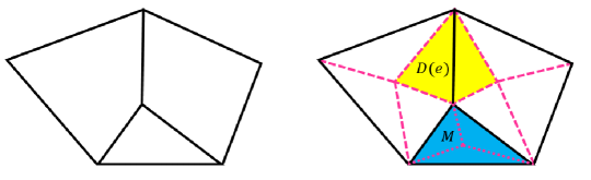
To begin with, we introduce the construction of staggered meshes, which lays foundation for the construction of finite element spaces suitable for our setting. Let be a shape-regular family of matching meshes covering exactly, where hanging nodes are allowed. Note that the shape-regularity for general polygonal meshes can be described as follows: (1) Every element is star-shaped with respect to a ball of radius , where is a positive constant and is the diameter of ; (2) For every element and every edge , it satisfies , where is a positive constant and represents the length of edge . For an element , we select an interior point and connect it to all the vertices of . The resulting sub-triangulation is denoted as . We remark that is an arbitrary point interior to and for simplicity we choose it as center point. The union of all the edges in the primal partition is denoted as . We use to represent the subset of , that is the set of edges in that does not lie on . In addition, the edges generated during the subdivision process due to the connection of the interior point to all the vertices are called dual edges, which is denoted as . In addition, we define and . For each triangle , we let be the diameter of and . Next, we introduce the dual mesh. For each interior edge , we use to represent the dual mesh, which is the union of the two triangles in sharing the common edge . For each edge , we use to denote the triangle in having the edge , see Figure 1 for an illustration. For each edge , we define a unit normal vector as follows: If is an interior edge, then is the unit normal vector of pointing towards the outside of . If is an interior edge, we then fix as one of the two possible unit normal vectors on . When there is no ambiguity, we use instead of to simplify the notation. Let be the order of approximation, for every and , we define and as the spaces of polynomials of degree less than or equal to on and , respectively.
For a scalar, vector, or tensor function that is double-valued on an interior edge , its jump and average on are defined as
where and are the two triangles belonging to which share the common edge . We set and on boundary edges.
Now we are ready to introduce the finite element spaces that will be used for the construction of our method. First, the locally conforming SDG space is defined by
which is equipped by the following norm
For a function we define .
Next, the locally -conforming SDG space is defined by
Finally, the locally conforming finite element space is defined as
We can derive the staggered DG discretization for the Biot system of poroelasticity by following [51, 53], which reads as follows: Find such that
| (3.1) | ||||
| (3.2) | ||||
| (3.3) | ||||
| (3.4) | ||||
| (3.5) |
where
and
The bilinear forms defined above satisfy the following adjoint properties
In addition, the following inf-sup condition holds; cf. [13].
| (3.6) |
and
| (3.7) |
Remark 3.1.
Now we prove the inf-sup condition, which is the key to proving the stability and convergence estimates of the proposed method. The methodology exploited here is different from that of [28]. Indeed the norm used here bypasses the construction of divergence free functions in proving the convergence estimates.
Lemma 3.1.
The following inf-sup condition holds
| (3.8) |
Proof.
To prove the inf-sup condition (3.8), we apply Fortin interpolation operator (cf. [5]), namely, we need to build an interpolation operator such that it satisfies for any
To this end we will first build such that it satisfies
| (3.9) |
then we correct by using which satisfies , in addition, there holds
| (3.10) | ||||
| (3.11) |
Since satisfies the inf-sup condition (3.7), which means there exists that satisfies
Next, we correct in the following way. We define the following spaces for each primal element :
For each primal element , we consider the stable approximation for the Stokes element such that
where denotes restricted to the primal element . We then solve for such that
Since on it is easy to check that the second equation also satisfies for a constant function. Here we remark that the existing stable pair that fits into the above spaces can be Taylor-Hood element (cf. [7]).
Let , then we can check that
which satisfies (3.10) by summing over all the primal elements. Here denotes the space restricted to each primal element . In addition, it also holds
Therefore, we have built and which satisfy (3.9)-(3.11). Hence, by the well-known arguments from [5] we can infer that the existence of and leads to the inf-sup condition.
∎
Remark 3.2.
In the above proof, we employ Taylor-Hood stable pair, in fact we can also exploit Scott-Vogelius element. In which case, we need to be careful about the singular nodes, indeed if singular nodes exists then one needs to enforce additional restriction on those nodes (cf. [21]), which is naturally satisfied for our choice of space .
We also emphasize that we choose locally -conforming space for to enforce the symmetry of stress, which is different from that of [28]. In fact, we can also exploit fully discontinuous space for , which then leads to strongly symmetric stress. In this case, the final system will be singular for rectangular mesh if one chooses the center point as . One can perturb the position of to avoid singularity. We want to develop a numerical scheme which is stable regardless of the position of , thus we choose locally -conforming space for .
In order to prove the well-posedness of (3.1)-(3.5), we will make use of the following theorem; cf. [43].
Theorem 3.1.
Let the linear, symmetric and monotone operators be given for the real vector space to its dual algebraic dual , and let be the Hilbert space which is the dual of with the seminorm
Let be a relation with domain . Assume is monotone and . Then for each and for each , there is a solution of
| (3.12) |
with
Proof.
In order to fit (3.1)-(3.5) in the form of Theorem 3.1, we consider a slightly modified formulation, with (3.1) differentiated in time and the new variables and representing and , respectively:
| (3.13) |
We now introduce the operators
We have a system in the form of (3.12), where
and .
The dual space is , and the condition in Theorem 3.1 allows for non-zero source terms only in the equations with time derivatives, which means . We can reduce our problem to a system with by solving for each an elasticity problem with a source term , cf. [42].
Subtracting the above equations from (3.1)-(3.5), we can obtain
| (3.14) | ||||
| (3.15) | ||||
| (3.16) | ||||
| (3.17) | ||||
| (3.18) |
which results in a problem with a modified right hand side .
The range condition can be verified by showing that the square finite dimensional homogeneous system: Find such that
| (3.19) | ||||
| (3.20) | ||||
| (3.21) | ||||
| (3.22) | ||||
| (3.23) |
has only zero solution. Taking in (3.19)-(3.23) and summing up the resulting equations yield
which gives and . By the inf-sup condition (3.6), we have
thereby by using the discrete Poincaré-Friedrichs inequality (cf. [6]), consequently, . The inf-sup condition (3.8) and (3.19) lead to
which yields and .
Finally, we need compatible initial data , i.e., . Let us first consider the initial data for the discrete formulation (3.1)-(3.5). We take to be the elliptic projection of the initial data for the weak formulation (2.5)-(2.9), which is constructed from by the procedure described at the end of section 2. With the reduction to a problem with , the construction satisfies . Then by
we have . For the initial data of the differentiated problem (3.13), (3.2)-(3.5), we simply take , which also satisfies . Here and are not needed for the differentiated problem, but will be used to recover the solution of the original problem.
Now all conditions of Theorem 3.1 are satisfied and we conclude the existence of a solution of (3.13), (3.2)-(3.5) with and . By taking in (3.4) and using that and satisfy (3.4) at , we also infer that .
Next, we recover the solution of the original problem. Let us define
By construction, and . Integrating (3.13) from to any and using that satisfy (3.1) at , we conclude that (3.1) holds for all . This completes the existence proof. Uniqueness follows from the stability bound given in Theorem 4.1 in the next section.
∎
Before closing this section, we introduce some interpolation operators which will play an important role for later analysis. There exists the interpolation operator satisfying for any
| (3.24) |
Similarly, there also exists an operator such that for any
| (3.25) |
The definition of the interpolation operators implies that
| (3.26) | ||||
| (3.27) |
In addition for and , we also have
| (3.28) | ||||
| (3.29) |
It is easy to check that and are polynomial preserving operators, which satisfy the following interpolation error estimates (cf. [17, 13])
| (3.30) |
In addition, we take to be the standard nodal interpolation operator, which satisfies
| (3.31) |
4 Error analysis
In this section, we prove the convergence estimates for the semi-discrete scheme and fully discrete scheme with backward Euler in time. In particular we will show that the stability and convergence error estimates are independent of the anisotropy ratio and of the storativity coefficient , and are valid for .
4.1 Error analysis for semi-discrete scheme
In this subsection we prove the stability and convergence estimates for the semi-discrete scheme. To begin, we consider the following stability estimate.
Proof.
Differentiating (3.1) in time, taking in (3.1)-(3.5) and summing up the resulting equations yield
Integrating over time implies
The Cauchy-Schwarz inequality and Young’s inequality lead to
| (4.1) |
By (3.1) and the inf-sup condition (3.8), we have
Then an appeal to the discrete Poincaré-Friedrichs inequalities gives
| (4.2) |
Taking , and in (3.1)-(3.3), and summing up the resulting equations, we deduce that
| (4.3) |
Thus, we can infer from (4.2) and (4.3) that
Choosing small enough yields
| (4.4) |
On the other hand, we have from (3.4) and the inf-sup condition (3.6)
| (4.5) |
Combining the discrete Poincaré-Friedrichs inequalities, (4.4) and (4.5) lead to
| (4.6) |
Therefore, choosing small enough, we can infer from (4.1), (4.5) and (4.6) that
| (4.7) |
Next, differentiating (3.1)-(3.4) in time and combining them with (3.5) with the choices , we can obtain
| (4.8) |
Then by inf-sup condition (3.8) and (3.1) differentiated in time, we have
| (4.9) |
Choosing in (4.8) small enough yields
which coupling with (4.7) leads to
Since the discrete initial data is the elliptic projection of the initial data , we have
| (4.10) |
Therefore, the proof is completed.
∎
Next, we will prove the convergence estimate. To simplify the notation, we let
Theorem 4.2.
Proof.
We obtain the following error equations by replacing by and performing integration by parts on (3.1)-(3.5)
| (4.11) | ||||
| (4.12) | ||||
| (4.13) | ||||
| (4.14) | ||||
| (4.15) |
for .
Differentiating (4.11) with time, taking , and summing up the resulting equations yield
| (4.16) |
It follows from (3.26) and (3.27) that
In addition, the Cauchy-Schwarz inequality yields
Therefore, we have from (4.16) that
Integrating in time from to an arbitrary results in
| (4.17) |
It follows from the inf-sup condition (3.8) and (4.11) that
| (4.18) |
Taking in (4.11)-(4.13), and summing up the resulting equations yield
which together with Young’s inequality implies
Taking small enough and using (4.18), we can obtain
| (4.19) |
It follows from (3.6) and (4.14) that
| (4.20) |
which together with the discrete Poincaré-Friedrichs inequalities implies
An application of (4.19) and (4.20) leads to
Besides, we can infer from (4.18) and (4.19) that
Choosing and in (4.17) small enough, we can infer from the preceding arguments
| (4.21) |
Differentiating (4.11)-(4.14) in time and setting , we can obtain
Integrating over time and using yield
| (4.22) |
By inf-sup condition (3.8) and (4.11) differentiated in time, we can obtain
Choosing and in (4.22) small enough leads to
which can be combined with (4.18), (4.19), (4.20) and (4.21) implies
The initial data satisfies
| (4.23) |
Therefore, the proof is completed by combining the preceding arguments and the interpolation error estimates (3.30)-(3.31).
∎
Remark 4.1.
(robustness of error estimates for nearly incompressible materials). We can observe from the above proof that we employ the coercivity of , while the coercivity of on is not uniform in . Indeed,
holds with a constant but as . It means that our error estimates obtained using the coercivity of may have error bounds growing unboundedly as . In order to get a uniform bound, we can follow the framework given in [28, 53], which is omitted for simplicity. In fact, proceeding analogously to [28, 53] we can check that our proposed method has uniformly bounded estimate.
4.2 Error analysis for fully discrete scheme
In this subsection we analyze the convergence estimates for the fully discrete scheme. To this end we introduce a partition of the time interval into subintervals and denote the time step size by . Using backward Euler scheme in time, we get the fully discrete staggered DG method as follows: Find such that
| (4.24) | ||||
| (4.25) | ||||
| (4.26) | ||||
| (4.27) | ||||
| (4.28) |
for .
For a Sobolev space on with a norm , we define the discrete in time norms by
and we let
Theorem 4.3.
Proof.
Since (4.24)-(4.24) is a square linear system, uniqueness implies existence. It suffices to show the uniqueness. To this end, suppose and the th time step solution vanishes. Then we have from (4.24)-(4.28)
| (4.29) | ||||
| (4.30) | ||||
| (4.31) | ||||
| (4.32) | ||||
| (4.33) |
Taking in (4.29)-(4.33) and summing up the resulting equations yield
thereby and .
∎
Theorem 4.4.
Proof.
We have the following error equations by performing integration by parts on (4.24)-(4.28)
| (4.34) | |||
| (4.35) | |||
| (4.36) | |||
| (4.37) | |||
| (4.38) |
for .
Consider (4.34) at iterations and and taking the difference, then setting in the difference equation and (4.35)-(4.38), and summing up the resulting equations, we have
Using the inequality and the Cauchy-Schwarz inequality, we can obtain
| (4.39) |
It follows from (3.6), (4.37) and the discrete Poincaré-Friedrichs inequality that
| (4.40) |
Similarly, we can infer from (3.8) and (4.34) that
| (4.41) |
Besides, taking in (4.34)-(4.36) and summing up the resulting equations yield
then an application of Young’s inequality yields
| (4.42) |
Choosing small enough and combining with (4.40), (4.41) give
| (4.43) |
On the other hand, we have from Taylor’s expansion
where the right hand side can be estimated by the Cauchy-Schwarz inequality
Similarly, we have
Therefore, we can infer from (4.39) and Young’s inequalities that
| (4.44) |
Changing to in (4.39) and summing over , we can obtain
| (4.45) |
It follows from the interpolation error estimates (3.30)-(3.31) that
The Cauchy-Schwarz inequality and the interpolation error estimates (3.30) imply
| (4.46) |
Discrete integration by parts in time yields
where the last term can be estimated by
Thus, the preceding arguments lead to
Considering (4.34)-(4.37) at iterations and , and taking the difference, setting and summing up the resulting equations yield
We can infer from inf-sup condition (3.6) and (3.8) that
Therefore, we have
Changing to and summing over , we can obtain
Proceeding analogously to (4.46), we can get
Combining the above estimates with the interpolation error estimates (3.30)-(3.31) completes the proof.
∎
5 Fixed stress splitting scheme
The global system (4.24)-(4.28) consists of five variables which is relatively large. In order to reduce the computational costs, we propose the following fixed stress splitting scheme inspired by [30]. This includes two steps: First, the flow problem is solved independently. Second, the mechanics problem is solved using updated pressure and flux. For fixed , the detailed splitting scheme reads as follows:
Step 1: Given , find such that
| (5.1) | |||
| (5.2) |
Step 2: Given , find such that
| (5.3) | ||||
| (5.4) | ||||
| (5.5) |
The initial guess for the iterations is chosen to be the solution at the last time step, i.e., .
Remark 5.1.
Theorem 5.1.
Proof.
Taking , in the above equations, and summing up the resulting equations, we can infer that
| (5.7) |
Consider (5.3)-(5.4) at iterations and and take the difference, setting and summing up the resulting equations yield
which leads to
Thus, we have
| (5.8) |
We can infer from (5.7), the equality and the identity that
Therefore, an appeal to (5.8) yields
It follows from the inf-sup condition (3.6) and the discrete Poincaré-Friedrichs inequality that
where is the Poincaré constant and is the inf-sup constant in (3.6). Thereby, if we require
then there holds
| (5.9) |
which leads to the desired estimate (5.6).
∎
6 Numerical experiments
In this section we present several numerical experiments to verify the theoretical convergence rates and illustrate the behavior of the proposed method. We also present one benchmark example showing the locking-free property of the method. In the simulation presented below, we use the polynomial order .
6.1 Smooth solution test
In this example, we test the convergence of our method. To this end, we set , where the displacement and pressure are given by
The corresponding and can be calculated by (2.1)-(2.3). We set and the simulation time is with time steps . We remark that should be chosen small enough so that the time discretization error will not influence the convergence rates. For this example, we consider two values of , i.e., and
| (6.3) |
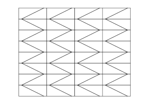
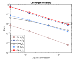
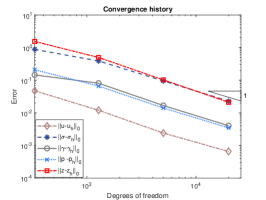
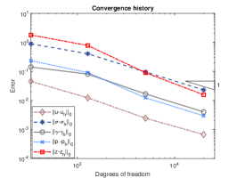
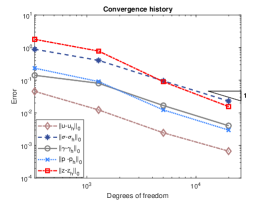
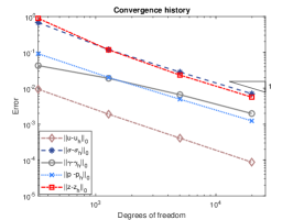
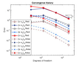
We exploit square meshes and trapezoidal meshes for this example, see Figure 2 for an illustration. The convergence history against the number of degrees of freedom for rectangular meshes and trapezoidal meshes with various values of is depicted in Figure 3. Optimal convergence rates matching the theoretical results can be obtained for various values of . In addition, with different values of , the accuracy for all the errors remain almost the same and the method is still valid for . Further, the accuracy for errors of on rectangular meshes and trapezoidal meshes is slightly different. Figure 4 shows the convergence history on rectangular meshes for anisotropic defined in (6.3) and similar performances can be observed, which illustrates the robustness of our method to the anisotropy ratio.


6.2 Cantilever bracket benchmark problem
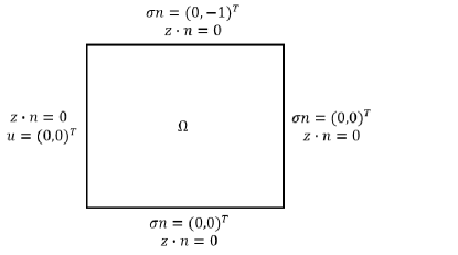
The computational domain is the unit square. We impose no-flow boundary condition along all sides. The deformation is fixed at the left edge, and a downward traction is applied along the top. The bottom and right sides are traction-free, see Figure 5 for an illustration of the boundary condition. The time step for this example is .
We use the same physical parameters as in [39] as they typically induce locking:
where is the Young’s modulus and is the Poisson ratio, and the Lamé parameters are computed by
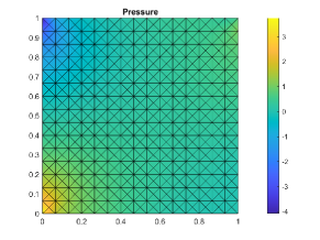
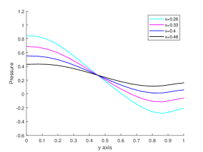
Figure 6 shows that our proposed method yields a smooth pressure field, in contrast to the non-physical checkboard pattern that one obtains with continuous elasticity elements at the early time steps, see [39]. In addition, Figure 6 also indicates that the pressure solution along different -lines at time . We can observe that it is free of oscillations and our solution agrees with the one obtained by DG-mixed discretizations [39].
6.3 Anisotropic meshes
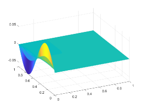
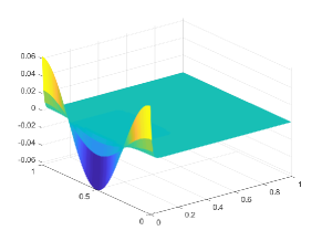
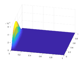
The computational domain is taken to be and we set . The simulation time is with time steps . The exact displacement and pressure are given as
The used meshes are of Shishkin type (cf. [2]), see the example in Figure 8. For a parameter they are constructed by choosing a transition point parameter and generating a grid of points by
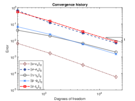
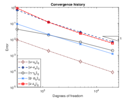
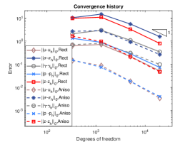
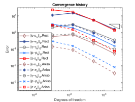
The transition point parameter is chosen as . Here we choose and the corresponding exact velocity and pressure at are displayed in Figures 7 and 8, where the exponential boundary layer near is clearly visible. The layer has a width of and is present in the velocity and pressure solution. The convergence history against the number of degrees of freedom for various values of is shown in Figure 9 on square meshes and anisotropic meshes. We can observe that optimal convergence rates matching the theoretical results can be obtained, which indicates that our method can work well on anisotropic meshes and the method works for . Further, the errors on anisotropic meshes are much smaller than that of rectangular meshes, which illustrates the superior performances of anisotropic meshes in particular for layered problem.

6.4 A model problem of vertical compaction
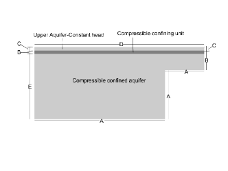
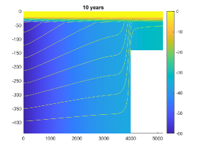
In this example, we consider a more practical case motivated by the example given in [25], where three sedimentary layers overlying an impermeable bedrock in a basin. The sediment stack totals 420m at the deepest point of the basin (m) but thins to 120m above the step (m). The top two layers of the sequence are 20m thick each, see Figure 10 for an illustration of the domain geometry. The first and third layers are aquifers; the middle layer is relatively impermeable to flow. The flow field initially is at steady state, but pumping from the lower aquifer reduces hydraulic head by 6m per year at the basin center. The head drop moves fluid away from the step. The fluid supply in the upper reservoir is limitless. The initial condition is set to zero and the boundary conditions for region A to E are described in Table 1, in addition, we let . The values for the parameters are given in Table 2. The final simulation time is 10 years, where we take the simulation time to be . Figure 11 shows the plot for pressure and displacement at 2 years and 10 years.

| A | ||
|---|---|---|
| B | ||
| C | ||
| D | ||
| E |
| Variable | Description | Value |
|---|---|---|
| storage coefficient, aquifer layers | ||
| storage coefficient, confining layers | ||
| permeability, aquifer layers | 25 m/day | |
| permeability, confining layers | 0.01 m/day | |
| Biot-Willis coefficient | 1 | |
| E | Young’s modulus, aquifer layers | Pa |
| E | Young’s modulus, confining layers | Pa |
| Poisson ratio, all regions | 0.25 | |
| Declining head boundary | (6 m/year) |

7 Conclusion
In this paper we analyzed a staggered DG method for a five-field formulation of the Biot system of poroelasticity on general polygonal meshes. The method is proved to converge in optimal rates for all the variables in their natural norms. In addition, the error estimates are independent of the storativity coefficient and are valid even for , which is also confirmed by our numerical simulation. Several numerical experiments including cantilever bracket benchmark problem are presented, which further confirms the locking-free property of our method. In addition, the accuracy of our method is slightly influenced by the shape of the grid. Numerical results illustrate that our method is a good option for solving problems on anisotropic meshes. Moreover, our method can handle nonmatching meshes straightforwardly, which is advantageous in solving problem with local features. In the future we will extend this method to solve nonlinear poroelasticity.
Acknowledgment
The research of Eric Chung is partially supported by the Hong Kong RGC General Research Fund (Project numbers 14304719 and 14302018) and CUHK Faculty of Science Direct Grant 2019-20 and NSFC/RGC Joint Research Scheme (Project number HKUST620/15). The research of Eun-Jae Park was supported by the National Research Foundation of Korea (NRF) grant funded by the Ministry of Science and ICT (NRF-2015R1A5A1009350 and NRF-2019R1A2C2090021).
References
- [1] I. Ambartsumyan, E. Khattatov, and I. Yotov. A coupled multipoint stress – multipoint flux mixed finite element method for the Biot system of poroelasticity. arXiv:2001.04582, 2020.
- [2] T. Apel, A. Linke, and C. Merdon. A nonconforming pressure-robust finite element method for the Stokes equations on anisotropic meshes. arXiv:2002.12127, 2020.
- [3] M. A. Biot. General theory of three‐dimensional consolidation. J. Appl. Phys., 12(2):155–164, 1941.
- [4] D. Boffi, M. Botti, and D. A. Di Pietro. A nonconforming high-order method for the Biot problem on general meshes. SIAM J. Sci. Comput., 38(3):A1508–A1537, 2016.
- [5] D. Braess. Finite Elements: Theory, Fast Solvers, and Applications in Solid Mechanics. Cambridge University Press, 2007.
- [6] S. C. Brenner. Poincaré-Friedrichs inequalities for piecewise functions. SIAM J. Numer. Anal., 41(1):306–324, 2003.
- [7] F. Brezzi and R. S. Falk. Stability of higher-order Hood-Taylor methods. SIAM J. Numer. Anal., 28(3):581–590, 1991.
- [8] S. Cheung, E. T. Chung, H. H. Kim, and Y. Qian. Staggered discontinuous Galerkin methods for the incompressible Navier–Stokes equations. J. Comput. Phys., 302(1):251–266, 2015.
- [9] E. T. Chung, B. Cockburn, and G. Fu. The staggered DG method is the limit of a hybridizable DG method. SIAM J. Numer. Anal., 52(2):915–932, 2014.
- [10] E. T. Chung, B. Cockburn, and G. Fu. The staggered DG method is the limit of a hybridizable DG method. Part II: The Stokes flow. J. Sci. Comput., 66(2):870–887, 2016.
- [11] E. T. Chung, J. Du, and C. Lam. Discontinuous Galerkin methods with staggered hybridization for linear elastodynamics. Comput. Math. Appl., 74(6):1198–1214, 2017.
- [12] E. T. Chung and B. Engquist. Optimal discontinuous Galerkin methods for wave propagation. SIAM J. Numer. Anal., 44(5):2131–2158, 2006.
- [13] E. T. Chung and B. Engquist. Optimal discontinuous Galerkin methods for the acoustic wave equation in higher dimensions. SIAM J. Numer. Anal., 47(5):3820–3848, 2009.
- [14] E. T. Chung, H. H. Kim, and O. B. Widlund. Two-level overlapping Schwarz algorithms for a staggered discontinuous Galerkin method. SIAM J. Numer. Anal., 51(1):47–67, 2013.
- [15] E. T. Chung and C. Lee. A staggered discontinuous Galerkin method for the curl–curl operator. IMA J. Numer. Anal., 32(3):1241–1265, 2012.
- [16] E. T. Chung and W. Qiu. Analysis of an SDG method for the incompressible Navier–Stokes equations. SIAM J. Numer. Anal., 55(2):543–569, 2017.
- [17] P. G. Ciarlet. The Finite Element Method for Elliptic Problems. Society for Industrial and Applied Mathematics, 2002.
- [18] J. Du and E. T. Chung. An adaptive staggered discontinuous Galerkin method for the steady state convection–diffusion equation. J. Sci. Comput., 77(3):1490–1518, 2018.
- [19] G. Fu. A high-order HDG method for the Biot’s consolidation model. Comput. Math. Appl., 77(1):237–252, 2019.
- [20] F. J. Gaspar, F. J. Lisbona, and P. N. Vabishchevich. A finite difference analysis of Biot’s consolidation model. Appl. Numer. Math., 44(4):487–506, 2003.
- [21] J. Guzmán and L. R. Scott. The Scott-Vogelius finite elements revisited. Math. Comp., 88(316):515–529, 2019.
- [22] X. Hu, L. Mu, and X. Ye. Weak Galerkin method for the Biot’s consolidation model. Comput. Math. Appl., 75(6):2017–2030, 2018.
- [23] H. H. Kim, E. T. Chung, and C. Lee. A staggered discontinuous Galerkin method for the Stokes system. SIAM J. Numer. Anal., 51(6):3327–3350, 2013.
- [24] J. Korsawe and G. Starke. A least-squares mixed finite element method for Biot’s consolidation problem in porous media. SIAM J. Numer. Anal., 43(1):318–339, 2005.
- [25] S. A. Leake and P. A. Hsieh. Simulation of deformation of sediments from decline of ground-water levels in an aquifer underlain by a bedrock step. U.S. Geological Survey Open File Report: 97-47, 1997.
- [26] J. J. Lee. Robust error analysis of coupled mixed methods for Biot’s consolidation model. J. Sci. Comput., 69(2):610–632, 2016.
- [27] J. J. Lee. Robust three-field finite element methods for Biot’s consolidation model in poroelasticity. BIT Numer. Math, 58(2):347–372, 2018.
- [28] J. J. Lee and H. H. Kim. Analysis of a staggered discontinuous Galerkin method for linear elasticity. J. Sci. Comput., 66(2):625–649, 2016.
- [29] J. J. Lee, K.-A. Mardal, and R. Winther. Parameter-robust discretization and preconditioning of Biot’s consolidation model. SIAM J. Sci. Comput., 39(1):A1–A24, 2017.
- [30] A. Mikelić and M. F. Wheeler. Convergence of iterative coupling for coupled flow and geomechanics. Comput. Geosci., 17(3):455–461, 2013.
- [31] M. A. Murad and A. F. D. Loula. Improved accuracy in finite element analysis of Biot’s consolidation problem. Comput. Methods Appl. Mech. Engrg., 95(3):359–382, 1992.
- [32] M. A. Murad and A. F. D. Loula. On stability and convergence of finite element approximations of Biot’s consolidation problem. Internat. J. Numer. Methods Engrg., 37(4):645–667, 1994.
- [33] M. A. Murad, V. Thomée, and A. F. D. Loula. Asymptotic behavior of semidiscrete finite-element approximations of Biot’s consolidation problem. SIAM J. Numer. Anal., 33(3):1065–1083, 1996.
- [34] C. Niu, H. Rui, and X. Hu. A stabilized hybrid mixed finite element method for poroelasticity. Comput. Geosci., 2020.
- [35] J. M. Nordbotten. Stable cell-centered finite volume discretization for Biot equations. SIAM J. Numer. Anal., 54(2):942–968, 2016.
- [36] R. Oyarzúa and R. Ruiz-Baier. Locking-free finite element methods for poroelasticity. SIAM J. Numer. Anal., 54(5):2951–2973, 2016.
- [37] P. J. Phillips and M. F. Wheeler. A coupling of mixed and continuous Galerkin finite element methods for poroelasticity I: the continuous in time case. Comput. Geosci., 11(2):131–144, 2007.
- [38] P. J. Phillips and M. F. Wheeler. A coupling of mixed and continuous Galerkin finite element methods for poroelasticity II: the discrete-in-time case. Comput. Geosci., 11(2):145–158, 2007.
- [39] P. J. Phillips and M. F. Wheeler. Overcoming the problem of locking in linear elasticity and poroelasticity: an heuristic approach. Comput. Geosci., 13(1):5–12, 2009.
- [40] C. Rodrigo, F. J. Gaspar, X. Hu, and L.T. Zikatanov. Stability and monotonicity for some discretizations of the Biot’s consolidation model. Comput. Methods Appl. Mech. Engrg., 298(1):183–204, 2016.
- [41] R. E. Showalter. Diffusion in poro-elastic media. J. Math. Anal. Appl., 251(1):310–340, 2000.
- [42] R. E. Showalter. Nonlinear degenerate evolution equations in mixed formulation. SIAM J. Numer. Anal., 42(5):2114–2131, 2010.
- [43] R. E. Showalter. Monotone operators in Banach space and nonlinear partial differential equations. American Mathematical Society, 2013.
- [44] M. Wheeler, G. Xue, and I. Yotov. Coupling multipoint flux mixed finite element methods with continuous Galerkin methods for poroelasticity. Comput. Geosci., 18(1):57–75, 2014.
- [45] S.-Y. Yi. A coupling of nonconforming and mixed finite element methods for Biot’s consolidation model. Numer. Methods Partial Differential Equations, 29(5):1749–1777, 2013.
- [46] S.-Y. Yi. Convergence analysis of a new mixed finite element method for Biot’s consolidation model. Numer. Methods Partial Differential Equations, 30(4):1189–1210, 2014.
- [47] S.-Y. Yi. A study of two modes of locking in poroelasticity. SIAM J. Numer. Anal., 55(4):1915–1936, 2017.
- [48] L. Zhao, E. T. Chung, and M. Lam. A new staggered DG method for the Brinkman problem robust in the Darcy and Stokes limits. Comput. Methods Appl. Mech. Engrg., 364(1), 2020.
- [49] L. Zhao, E. T. Chung, E.-J. Park, and G. Zhou. Staggered DG method for coupling of the Stokes and Darcy-Forchheimer problems. SIAM J. Numer. Anal., 2020, to appear.
- [50] L. Zhao, D. Kim, E.-J. Park, and E. Chung. Staggered DG method with small edges for Darcy flows in fractured porous media. arXiv:2005.10955, 2020.
- [51] L. Zhao and E.-J. Park. A staggered discontinuous Galerkin method of minimal dimension on quadrilateral and polygonal meshes. SIAM J. Sci. Comput., 40(4):A2543–A2567, 2018.
- [52] L. Zhao and E.-J. Park. A lowest-order staggered DG method for the coupled Stokes–Darcy problem. IMA J. Numer. Anal., 40(4):2871–2897, 2020.
- [53] L. Zhao and E.-J. Park. A staggered cell-centered DG method for linear elasticity on polygonal meshes. SIAM J. Sci. Comput., 42(4):A2158–A2181, 2020.
- [54] L. Zhao, E.-J. Park, and D. w. Shin. A staggered DG method of minimal dimension for the Stokes equations on general meshes. Comput. Methods Appl. Mech. Engrg., 345(1):854–875, 2019.