remarkRemark \newsiamremarkhypothesisHypothesis \newsiamthmclaimClaim \headersLog-concave Independent ComponentsS. Kubal, C. Campbell, and E. Robeva
Log-concave Density Estimation with Independent Components††thanks: Submitted July 26, 2025. \fundingElina Robeva was supported by an NSERC Discovery Grant DGECR-2020-00338.
Abstract
We propose a method for estimating a log-concave density on from samples, under the assumption that there exists an orthogonal transformation that makes the components of the random vector independent. While log-concave density estimation is hard both computationally and statistically, the independent components assumption alleviates both issues, while still maintaining a large non-parametric class. We prove that under mild conditions, at most samples (suppressing constants and log factors) suffice for our proposed estimator to be within of the original density in squared Hellinger distance. On the computational front, while the usual log-concave maximum likelihood estimate can be obtained via a finite-dimensional convex program, it is slow to compute – especially in higher dimensions. We demonstrate through numerical experiments that our estimator can be computed efficiently, making it more practical to use.
keywords:
density estimation, log-concave densities, sample complexity1 Introduction
A log-concave probability density on is of the form for a closed, proper, convex function . Log-concave density estimation is a type of non-parametric density estimation dating back to the work of Walther [37]. The class of log-concave distributions includes many known parametric families, has attractive statistical properties, and admits maximum likelihood estimates (MLE) that can be computed with established optimization algorithms [33]. Moreover, the MLE is ‘automatic’ in that no tuning parameters (such as kernel bandwidths) need to be chosen – a feature that can be especially useful in higher dimensions. However, log-concave density estimation suffers from the curse of dimensionality – one requires samples for the log-concave MLE in to be close to the true density in squared Hellinger distance [24]. Furthermore, the log-concave MLE is too slow to compute for large values of (e.g., and ).
We reduce the family of log-concave densities by assuming that the components of the random vector at hand become independent after a suitable orthogonal transformation is applied – an independent components assumption. While the family that we study is somewhat restrictive, it includes all multivariate normal distributions, and is still non-parametric. Furthermore, the independent components assumption provides a link with independent component analysis (ICA) models, see Samworth and Yuan [32]. We propose an easy-to-compute estimator for this family of densities and show that the sample complexity rate is no longer exponential in the ambient dimension : with at most samples (up to constants and log factors), the estimate is within of the true density in squared Hellinger distance.
1.1 Prior work
Shape-constrained density estimation has a long history. Classes of shape-constrained densities that have previously been studied include non-increasing [18], convex [19], -monotone [5], -concave [14] and quasi-concave densities [25]. The log-concave class of densities was first studied in dimension 1 by Walther [37], and a concise description of the log-concave MLE in higher dimensions was given by Cule et al. [11]. Various statistical properties of the procedure were established by Schuhmacher and Dümbgen [34], Carpenter et al. [7], Kur et al. [27], and Barber and Samworth [6] amongst others. Log-concavity has also gained popularity in applications [4, 33].
Subclasses of log-concave densities have also been studied in the recent years for the purposes of reducing the computational and statistical complexities of estimation, and also because they are important on their own. In the 1-dimensional setting, Kim et al. [23] study the set of log-concave densities that are exponentials of concave functions defined by at most linear hyperplanes. In this case, they show that the statistical rate becomes parametric. Xu and Samworth [39] consider log-concave densities whose super-level sets are scalar multiples of a fixed convex body in , and establish univariate rates for estimation. Robeva et al. [30] consider maximum likelihood estimation for totally positive and log-concave densities, which correspond to random vectors whose components are highly positively correlated. They prove existence and uniqueness of the MLE and propose an algorithm for computing it, although the statistical rates for this estimator are still unknown. Next, Kubjas et al. [26] study the family of log-concave densities that factorize according to an undirected graphical model, also providing existence and uniqueness results for the MLE (when the graph is given and chordal) together with an algorithm. Sample complexity rates for this model have not been studied either.
Here, we study the subfamily of log-concave densities on obtained by transforming product densities through orthogonal maps. These correspond to random vectors whose coordinates become independent post some orthogonal transformation. The most similar family to ours was considered by Samworth and Yuan [32], who study the class of log-concave densities of random vectors whose coordinates become independent after a linear transformation (rather than just an orthogonal transformation). They show that the projection (in a Kullback-Leibler (KL) sense) of a (not necessarily log-concave) distribution satisfying the above independent components property, to the set of log-concave distributions, still satisfies the independent components property with the same linear transformation. They also provide a method to perform density estimation in this setting, although their algorithm does not guarantee convergence to a global optimum. On the statistical front, they prove consistency; to the best of our knowledge however, finite sample rates have not yet been established in this setting. By simplifying the model here, we are able to provide a very fast algorithm together with sample complexity upper bounds displaying univariate rates.
Towards applicability to real data for tasks such as clustering, we show that our estimator can be used in conjunction with the Expectation-Maximization (EM) algorithm [13] to estimate mixtures of densities from our subfamily – this is a semiparametric generalization of Gaussian mixtures. A similar application was proposed in Cule et al. [11], where they show that mixtures of general log-concave densities can work better than Gaussian mixtures. However, estimating a mixture of general log-concave densities can be very costly, particularly in higher dimensions. Plugging our proposed estimator instead, into the EM algorithm, yields a much faster computation.
1.2 Problem
Suppose is a zero-mean random vector in , with a (probability) density . We say that (or ) satisfies the orthogonal independent components property if there exists an orthogonal matrix such that the components of are independent. In this case, the joint density of can be expressed as the product
| (1) |
where each is a univariate density. We focus mainly on the case where is log-concave, which is equivalent in this setting to requiring log-concavity of . Our goal is to efficiently estimate from independent and identically distributed (iid) samples, given that it satisfies the orthogonal independent components property with some unknown .
By writing , we can interpret this setting as an independent component analysis (ICA) model, where is the vector of independent sources and is the so-called unmixing matrix. Although mixing matrices in ICA do not need to be orthogonal to begin with, a pre-whitening procedure [10] can transform the problem to such an orthogonal form.
Instead of estimating the “-dimensional” density directly, we would like to leverage the underlying structure provided by (1), which allows us to simplify (using a change-of-variables formula) as
| (2) |
Here, are the rows of , and we refer to them as independent directions of . Note that the model and the factorization in (2) are invariant under permuting the rows of and the corresponding components of , as well as under flipping their respective signs.
If is known beforehand – if it is provided by an oracle – the estimation problem is simplified, and one can use the following procedure:
In reality, the unmixing matrix is unknown, and one needs to estimate it. If the covariance matrix of has distinct, well-separated eigenvalues, then this can be done by Principal Component Analysis (PCA), which involves diagonalizing the sample covariance matrix of . Otherwise, certain ICA algorithms may be used to estimate provided some non-Gaussianity requirements are satisfied [3, 17]. We refrain from using the same samples for the unmixing matrix estimation and the density estimation steps. Instead, we split the samples into two subsets, and , and use different subsets for the two purposes in order to prevent potentially problematic cross-interactions.
Denote the (PCA or ICA) estimate of by . We always require to be an orthogonal matrix. Given enough samples, the rows of can be shown to be close to those of up to permutations and sign-flips. More precisely, there exists a permutation and signs such that for some threshold
As the factorization in (2) is invariant under such permutations and sign-flips, one can simply relabel and to proceed with the analysis.
From , we can follow a procedure analogous to that used to obtain the oracle-informed estimate of . Namely, we use the estimated independent directions and the projected samples onto each such direction to produce univariate estimates ; then we take the product of these estimates over (see Definition 2.4).
1.3 Summary of contributions
The main contribution of this work is an algorithm for density estimation in the setting of Section 1.2, for which we prove finite sample guarantees and demonstrate numerical performance in terms of estimation errors and runtimes. The proposed algorithm is recorded as Algorithm 1.
The theoretical analysis in Section 3 yields sample complexity bounds for our algorithm under various assumptions, which are listed in Table 1 and Table 2. Briefly, if the true density is log-concave and satisfies some moment assumptions in addition to the orthogonal independent components property, then it can be estimated efficiently. In particular, samples (up to constants and log factors) are sufficient for our proposed estimator to be within of in squared Hellinger distance with probability 0.99. If the density has some additional smoothness, the rate can be improved up to .
Since we referred to smoothness, a quick comparison with kernel density estimators (KDE) is in order. Recall that in dimension , a KDE typically requires the true density to have “smoothness of order ” in order to achieve a dimension-independent statistical rate. More precisely, for in the Sobolev space with , achieving an expected total variation error of requires samples [21] so that one needs to counter the curse of dimensionality. On the contrary, our smoothness assumptions (see Smoothness assumption S1 and Smoothness assumption S2) are “order one” in that we only require control on the first-order (and if available, the second-order) derivatives.
Computational experiments are presented in Section 4, where we demonstrate improved estimation errors (in squared Hellinger distance) and improved runtimes as compared to usual log-concave MLE. A key consequence of our fast algorithm is easy scalability to higher dimensions – we are able to estimate densities in within no more than a few seconds.
2 Set-up and algorithms
First, we establish some notation. For a random vector (e.g. ), the subscript labels the components of the vector in , whereas the superscript labels the iid samples (or copies). Consider a (probability) density , and suppose . Given a unit vector , define the -marginal to be the density of . Additionally, for any (measurable) map , define the pushforward to be the law of . For an invertible linear map , the pushforward has a density . As described in Section 1, we have the relationship for which one can write by identifying with the linear map it induces.
For any positive integer , define . We denote by the Euclidean norm on , and by and respectively the operator norm and the Frobenius norm on . The squared Hellinger distance between densities is defined as . Note that is a metric on the space of densities. In various proofs, we also use the Wasserstein-1 distance, written .
Finally, the symbols etc. stand for absolute (universal) constants that do not depend on any parameters of the problem. Also, their values may be readjusted as required in different statements. We also use constants etc. that depend only on the dimension .
Recall the zero-mean density , satisfying the orthogonal independent components property, and consider the split-up independent samples and as introduced in Section 1. Our procedure for estimating consists of two stages: (1) use the samples to estimate an unmixing matrix , and (2) use the samples to estimate the marginal densities of in the directions given by the (estimated) rows of . We expand on these below, starting with the unmixing matrix estimation.
For (with finite second moments), consider the covariance matrix . Since the components of are independent, the covariance of
is diagonal. Hence, the rows of are the (normalized) eigenvectors of , and PCA can be used to estimate these eigenvectors under the following non-degeneracy condition:
Moment assumption M1
The density has finite second moments, and the eigenvalues of the covariance matrix are separated from each other by at least . Heteroscedastic multivariate Gaussians , where has well-separated eigenvalues, satisfy M1, and so do uniform distributions supported on rectangles with distinct side lengths.
From samples , one can compute the empirical covariance matrix
| (4) |
which is symmetric and positive semi-definite. Diagonalizing it yields the PCA-based estimate of .
Definition 2.1 (PCA-based estimate of ).
Let , and defined as in (4). Denote by a set of orthonormal eigenvectors of . Then, the estimate is defined to be the orthogonal matrix whose rows are .
Remark 2.2.
Note that above is defined only up to permutations and sign-flips of the rows. This is consistent, nevertheless, with our earlier discussion on the invariance of the model with respect to these transformations.
By the concentration of about , and the Davis-Kahan theorem [40], the ’s can be shown to be good estimates of , provided is not too small (see Proposition 3.12).
Now consider the situation where the eigenvalues of are poorly separated, or possibly degenerate. PCA may fail to recover the independent directions in this case. Consider, for example, the extreme case of an isotropic uniform distribution on a cube in with . Here, any is an eigenvector of , whereas the independent directions are only the axes of the cube. When has such degenerate eigenvalues, one needs to use higher moments to infer the unmixing matrix , which is the key principle behind ICA.
Recall our model , where we think of as the latent variables. As it is common in the ICA literature to have the latent variables ‘standardized’ to be unit-variance, we define . This lets us rewrite , where the new mixing matrix is . By orthogonality of and the diagonal nature of , the columns of are just scaled versions of the original independent directions .
All ICA methods require some form of non-Gaussianity; following Auddy and Yuan [3], we require the following assumptions on and .
Moment assumption M2
For each , assume that and for some . Additionally, assume that the condition number for some .
Remark 2.3.
Note that since , one could alternatively frame Moment assumption M2 in terms of . In particular, we have that .
Auddy and Yuan [3] propose a variant of the FastICA algorithm [22] that produces an estimate of achieving the optimal sample complexity for computationally tractable procedures. To recover an estimate of , we first rescale the columns of to unit norm, and form a matrix from these rescaled columns. To account for the possible non-orthogonality of the columns of , we compute the singular value decomposition , and set .
Isotropic uniform and exponential densities, for example, satisfy Moment assumption M2, but Gaussians do not due to the non-zero kurtosis requirement. But recall that heteroscedastic Gaussians do satisfy Moment assumption M1. If the moment assumptions discussed here are too restrictive, one could use other algorithms such as Fourier PCA [17], which require weaker notions of non-Gaussianity. Our theory in the following sections is agnostic of the specific procedure used to estimate , and depends only on the estimation error.
Given , and hence the estimated independent directions , consider the second stage of the estimation procedure now – estimating the marginal densities of . Take the samples , which are independent of , and project them as
| (5) |
Conditional on , it holds that (almost surely in ), which follows from the independence between and . Univariate density estimation can then be used to estimate each marginal using the samples . When is log-concave in particular (which is the focus of this work), we use univariate log-concave MLE [37]. This procedure finally yields our proposed “plug-in” estimator.
Definition 2.4 (Proposed estimator).
Given estimated orthogonal independent directions
computed from , and univariate density estimates computed from , define the estimator
| (6) |
Note that the proposed estimate is just the oracle-informed estimate with replaced by (since ). Further note that if we did not split the samples to conduct covariance estimation and density estimation separately, the law of conditional on would no longer be .
We summarize the above discussion as Algorithm 1. Recall that we had assumed to be zero-mean in our set-up; in the general case, one requires an additional centering step which we include in Algorithm 1.
Notice that we have not specified the sample splitting proportion between and . This is a free parameter in our method, and can be optimized based on the statistical rates obtained in Section 3, or based on numerical tests as explored in Section 4.2. An equal split with seems to generally work well. Interestingly, we observe empirically that not splitting the samples, i.e. reusing the same samples for the two stages, can also work very well, and even beat the splitting version.
Finally, we have kept the estimation procedures for the unmixing matrix and the marginals unspecified in Definition 2.4 and Algorithm 1 for the sake of generality. The framework of our analysis allows for flexibility in the choice of these procedures. However, we do focus mainly on PCA, ICA, and log-concave MLE in the following sections, and refer to Algorithm 1 as the log-concave independent components estimator (LC-IC) in that case. In particular, we use the R package logcondens [31] for univariate log-concave MLE in Line 6 of Algorithm 1. This package plays an important role in the computational speed of our method.
3 Analysis and sample complexities
This section is organized as follows. Section 3.1 presents basic error bounds and a generic sample complexity result, where the estimators for the unmixing matrix and the marginals are left unspecified. Section 3.2 and Section 3.3 then consider specific estimators to provide concrete sample complexities. Section 3.4 derives stronger bounds under additional assumptions, and collects the various sample complexities. Finally, Section 3.5 considers the case of misspecified log-concavity.
3.1 Error bounds and generic sample complexities
We consider the oracle-informed estimator first. The analysis involved is also applicable to the proposed estimator.
Lemma 3.1 (Error bound on the oracle estimator).
Suppose is a zero-mean probability density on , satisfying the orthogonal independent components property with independent directions . Let be the oracle-informed estimator as defined in (3). We have the bound
Proof 3.2.
A direct calculation yields
Now define and note that . Bernoulli’s inequality gives that .
Lemma 3.1 says that the problem of bounding boils down to controlling the univariate estimation errors . For log-concave densities, Kim and Samworth [24] and Carpenter et al. [7] have already established results of this kind. We stay in a general setting for now, by deriving the sample complexity of the oracle estimator from the sample complexity of any univariate density estimation procedure that it invokes.
Definition 3.3 (Sample complexity of a univariate density estimator).
Let be a univariate probability density, and let be an estimator of computed from iid samples. For and , define the sample complexity of be be the minimal positive integer such that iid samples from are sufficient to give
Now, we can immediately express the sample complexity of the oracle estimator in terms of as a consequence of Lemma 3.1 and a union bound.
Corollary 3.4 (Sample complexity of the oracle-informed estimator).
Let be a zero-mean probability density on , satisfying the orthogonal independent components property. Let be the oracle-informed estimator computed from samples . Then, for any and , we have
with probability at least , whenever
Here, is the sample complexity of the univariate density estimator invoked by .
Having concluded the analysis of the oracle-informed estimator, we can now turn to the general setting. Here, we only have an estimate of , and hence, the estimation error needs to be taken into account. This contributes additional terms to the risk of the proposed estimator, as the theorem below shows. The proof can be found in Section A.1.
Theorem 3.5 (Error bound on the proposed estimator).
Suppose is a zero-mean probability density on , satisfying the orthogonal independent components property with independent directions . Let be the proposed estimator (Definition 2.4). We have the error bound
where .
Here, is an orthogonal matrix, because and are. The term in the bound of Theorem 3.5 warrants an analysis similar to the oracle-informed estimator. Since is a univariate density estimate of conditional on , bounds on univariate density estimation control this term, when applied in a conditional sense.
The second and third terms in the bound of Theorem 3.5 call for a notion of stability; measures how far the ‘rotated’ density gets from the original density . If Hellinger distance is stable with respect to small rotations of the density, then can be bounded effectively in terms of the operator norm , where is the identity matrix. This operator norm is then well-controlled by the unmixing matrix estimation error as
| (7) |
The next lemma demonstrates such stability for zero-mean log-concave densities.
Lemma 3.6 (Hellinger stability).
Let be a zero-mean log-concave density on , and let be any invertible matrix. Then,
where is the covariance matrix of , and the constant depends only on the dimension .
The proof involves the log-concave projection of Dümbgen et al. [15], particularly making use of its local Hölder continuity [6]. It is delayed to Section A.2. Note that Lemma 3.6 is quite general, as it only uses log-concavity of (with no additional smoothness requirements). However, Lemma 3.6 inherits a constant that typically depends at least exponentially in . Also, the exponent of contributes a dependence to our sample complexity bounds (see the first two rows of Table 2). Later in Section 3.4, we show that smoothness assumptions on can give stronger bounds.
The last bit to consider is the unmixing matrix estimation error. In the same spirit as the discussion on univariate density estimation above, we consider a generic estimator for now, with sample complexity defined as below.
Definition 3.7 (Sample complexity of an unmixing matrix estimator).
Let be a zero-mean probability density on satisfying the orthogonal independent components property. Let be an estimator of an unmixing matrix of , computed from iid samples. For and , define the sample complexity of to be the minimal positive integer such that iid samples from are sufficient to give
for some set of independent directions of .
Now, we state the main result of this section, which expresses the sample complexity of the proposed estimator (Definition 2.4) in terms of the sample complexities in Definition 3.3 and Definition 3.7. The proof is presented in Section A.3.
Theorem 3.8 (Generic sample complexity of the proposed estimator).
Let be a zero-mean log-concave density on , satisfying the orthogonal independent components property. Let be the proposed estimator computed from samples . Then, for any and , we have
with probability at least whenever
| (8a) | |||
| and | |||
| (8b) | |||
Here, and are respectively the sample complexities of the univariate density estimator and the unmixing matrix estimator invoked by . As before, is the covariance matrix of and is a constant that depends only on .
To obtain concrete sample complexities, one needs to choose specific estimation procedures. In Section 3.2, we consider univariate log-concave MLE and its boosted variant, and provide corresponding bounds on . In Section 3.3, we present standard bounds on for PCA- and ICA-based estimators of .
3.2 Univariate density estimation for the marginals
Recall that for each , we need to estimate the densities from samples . When is log-concave, an efficient as well as convenient option is log-concave MLE [33], which is in fact minimax optimal.
Proposition 3.9 (Sample complexity of univariate log-concave MLE [24]).
Let be a univariate log-concave density, and denote by the log-concave MLE computed from iid samples from . Given and , we have
with probability at least whenever
for absolute constants .
In terms of Definition 3.3, we can restate this as . Notice that the right-hand side does not depend on , and as a result, the same upper bound also holds for the term from Theorem 3.8
The statement above is a “high-probability” variant of Theorem 5 of Kim and Samworth [24], and we provide a proof in Section A.4. Note that while the dependence is optimal, the dependence in the sample complexity could be improved. A standard way to do this is via boosting. The following definition uses the boosting technique from Algorithm A of Lovász and Vempala [28].
Definition 3.10 (Boosted univariate log-concave MLE).
Let , and suppose we have access to iid samples from a univariate log-concave density . Additionally, fix . The boosted estimator at error threshold is defined via the following procedure:
-
1.
Split the samples into batches of size , and denote by () the log-concave MLE computed from the samples in batch .
-
2.
For each batch , count how many other batches satisfy .
-
3.
If there exists a batch for which this number is larger than , return . Otherwise, return .
As the next proposition show, the sample complexity of the boosted log-concave MLE depends only logarithmically on , which is much milder. See Section A.5 for the proof.
Proposition 3.11 (Sample complexity boosted univariate log-concave MLE).
Let be a univariate log-concave density, and fix . Denote by the boosted log-concave MLE at error threshold , computed from independent batches of iid samples from each. Given , we have
with probability at provided
for absolute constants .
In particular, by multiplying the bounds for and , we get that the sample complexity
. As before, the right-hand side does not depend on .
3.3 Unmixing matrix estimation
Here, we discuss standard techniques for estimating , and show closeness of and . Recall that the methods used here for estimating – PCA or ICA – require different assumptions on the moments of (or ) in order to yield bounds on the estimation errors.
Consider regular PCA first. The PCA estimate of was obtained by computing the eigenvectors of the sample covariance matrix . Bounding the sample complexity of this estimation procedure is standard, and can be broken down into two simple steps: (i) bounding the distance between the empirical covariance matrix and the true covariance matrix , and (ii) bounding the distances between their corresponding eigenvectors. The result is summarized in the following proposition, the proof of which is delayed to A.6.
Proposition 3.12 (Sample complexity of estimating by PCA).
Let be a zero-mean, log-concave probability density on . Let be samples, and suppose Moment assumption M1 is satisfied with eigenvalue separation . Let and , and define . If
| (9) |
where are absolute constants, then with probability at least , PCA recovers vectors such that
up to permutations and sign-flips.
The right-hand side of (9) is an upper bound on sample complexity of the PCA-based estimator, for . The term is needed in order to allow the result above to hold for all positive , instead of just small values of .
As discussed earlier, assumptions on strict eigenvalue separation can be stringent, and possibly unrealistic in practical settings. In such cases, should be estimated by ICA instead, for which we have a result similar to Proposition 3.12.
Recall the definitions of and from Section 2, and express . The algorithm of Auddy and Yuan [3] then estimates the columns of , which coincide with up to scalings and signs.
The proposition below is a direct consequence of Theorem 3.4 of Auddy and Yuan [3], and provides an upper bound on for . The proof is delayed to Section A.7.
Proposition 3.13 (Sample complexity of estimating by ICA [3]).
Let be a zero-mean probability density on satisfying the orthogonal independent components property. Suppose, additionally, that Moment assumption M2 is satisfied with parameters and . Given and , and samples , if
| (10) |
for constants depending on , then with probability at least , ICA recovers vectors such that
for independent directions of .
The result above relies on non-zero excess kurtosis of the components of , which may be interpreted as a measure of non-Gaussianity. However, there exist distributions which differ from Gaussians only in higher cumulants. Techniques such as Fourier PCA [17] allow for estimating in such cases. As discussed earlier, our theory is agnostic to specific choices of ICA algorithms.
3.4 Stronger bounds under additional assumptions
While the statement of Theorem 3.8 is quite general, the inequality in (8b) contains a constant that typically depends at least exponentially in . This is owed to the stability result Lemma 3.6, which uses only the log-concavity of . Stronger stability inequalities are possible when is smooth.
In what follows, we consider two possible assumptions on the smoothness of . The choice of assumptions then allows us to quantify stability in either Kullback-Leibler (KL) divergence or total variation distance first, before translating this to stability in Hellinger distance. Let be a probability density on with mean zero.
Smoothness assumption S1
The density has finite second moments, is continuously differentiable, and the integral . The function is finite-valued everywhere, and belongs to the Hölder space for some , i.e.
| (11) |
Note that is commonly known as the score function, whose regularity also plays a role in sampling theory. We may also interpret (11) as a modified Hölder condition on . This assumption yields good stability in KL divergence, but it can be stringent since it requires, in particular, that is strictly positive everywhere. The following assumption relaxes this.
Smoothness assumption S2
The density has finite second moments, and has a (weak) gradient , with
| (12) |
This assumption yields a stability estimate in total variation distance (or equivalently, distance). Note that is not required to be differentiable in the strong sense, and hence, can have “corners” or “kinks”. But, jumps are still not allowed. An interesting example is the exponential-type density . Also, to compare with assumption S1, note that if with , then we write which can translate to a bound on .
Assumptions S1 and S2 can be interpreted better by considering a multivariate Gaussian distribution with density
where is the normalizing constant. Here, is clearly , with . On the other hand, , provided . We start with stability under Smoothness assumption S1.
Lemma 3.14 (Stability in KL).
Let be a zero-mean probability density on , satisfying Smoothness assumption S1. Let be any orthogonal matrix. Then,
The proof involves a direct analysis of the KL integral, using the bound . It is delayed to Section A.8. This result translates to Hellinger distance via the upper bound [16]
We remark that the exponent of in Lemma 3.14 is significantly higher than the corresponding exponent in Lemma 3.6, and this leads to better convergence rates as . In particular, this contributes an dependence to our sample complexity bounds, as compared to (see the rows of Table 2 corresponding to S1). We note that using higher derivatives of (provided for ) in the proof could potentially lead to even faster convergence. Next, we move on to stability under Smoothness assumption S2.
Lemma 3.15 (Stability in TV).
Let be a zero-mean probability density on , satisfying Smoothness assumption S2. Let be invertible with . Then,
The proof is based on bounding the Wasserstein-1 distance between and , accompanied by an argument inspired from Chae and Walker [8] (see Section A.9). Again, the bound can be translated to Hellinger distance via the inequality [16]
Finally, in the case of orthogonal matrices, the parameter .
Notice that the exponent of in Lemma 3.15 is again – the same as in Lemma 3.6. This contributes an dependence to our sample complexity bounds (see the rows of Table 2 corresponding to S2). A better exponent could potentially be obtained by requiring control on higher order Sobolev norms and following estimates from KDE theory [21].
We can now state the analogue of Theorem 3.8 under these stronger stability results. The proof is provided in Section A.10.
Corollary 3.16 (Sample complexities under smoothness assumptions).
Let be a zero-mean probability density on , satisfying the orthogonal independent components property. Let be the proposed estimator computed from samples . Then, for any and , we have
with probability at least whenever
| (13a) | |||
| and | |||
| (13b) | |||
Here, and are respectively the sample complexities of the univariate density estimator and the unmixing matrix estimator invoked by .
As stated, Corollary 3.16 does not require log-concavity of . If is smooth enough but not log-concave, the univariate density estimation stage of the proposed estimator can be done via kernel density estimation (KDE), for example, which would have a different sample complexity .
| Setting | Number of samples |
|---|---|
| Log-concave MLE | |
| Boosted log-concave MLE | |
| Adapted log-concave MLE |
| Setting | Number of samples |
|---|---|
| PCA | |
| ICA | |
| PCA, S1 | |
| ICA, S1 | |
| PCA, S2 | |
| ICA, S2 |
A different way in which we get stronger bounds under additional assumptions is adaptation. A univariate density is said to be log--affine, for some , if is piece-wise affine with at most pieces on the support of . Kim et al. [23] established parametric sample complexity of the log-concave MLE when the true density is log--affine with fixed. The following an immediate consequence of their Theorem 3.
Proposition 3.17 (Adaptation of log-concave MLE [23]).
Let be a log-concave density that is log--affine for some , and denote by the log-concave MLE computed from iid samples from . Given and , we have
with probability at least whenever
for an absolute constant .
As a consequence, we have that is at most up to log factors when is log--affine. The -dependence is due to Markov’s inequality, and may be improved to via boosting as before (see Definition 3.10).
We conclude this discussion by collecting some concrete bounds on the number of samples and that are sufficient for the proposed estimator to achieve with probability at least . These depend on the particular procedures invoked for marginal estimation and unmixing matrix estimation, as well as on the smoothness assumptions. The bounds on are presented in Table 1, and those for are tabulated in Table 2. The results in both tables take to be a zero-mean, log-concave density on , satisfying the orthogonal independent components property.
3.5 Bounds under misspecification of log-concavity
Let be the set of probability distributions on satisfying and for every hyperplane . Identical to the setting of densities, we say that a zero-mean distribution satisfies the orthogonal independent components property if there exists an orthogonal matrix such that the components of are independent when .
To study the case of misspecification, we need the log-concave projection of Dümbgen et al. [15], which is a map from to the set of log-concave densities on , defined by
If is a zero-mean distribution in satisfying the orthogonal independent components property, we show below that our proposed estimator (invoking univariate log-concave MLE), computed from iid samples from , gets close to .
Theorem 3.18 (Error bound with misspecification of log-concavity).
Let be a zero-mean distribution in , satisfying the orthogonal independent components property with independent directions . Let be the proposed estimator computed from samples . We have the error bound
where .
See Section A.11 for the proof.
We can now obtain sample complexities; to get concrete bounds, we focus on the ICA case and recall Moment assumption M2 with parameters and . Given and , define the moment quantities
for .
Theorem 3.19 (Samplex complexity with misspecification of log-concavity).
Let be a zero-mean distribution in satisfying the orthogonal independent components property. Suppose that Moment assumption M2 is satisfied, , and for some . Let be the proposed estimator computed from samples , invoking univariate log-concave MLE and ICA. Then, for any and , we have
with probability at least whenever
and
Here, the constants depend on , the constant depends only on , and depends only on .
The proof is provided in Section A.12. The inequality for depends polynomially on , and this is due to the use of Markov’s inequality in the proof. If the distribution is sub-exponential, better tails bounds may be used, as discussed by Barber and Samworth [6].
4 Computational experiments
In this section, we demonstrate the performance of the log-concave independent components estimator (LC-IC, Algorithm 1) on simulated as well as real data. Section 4.1 compares the estimation errors and runtimes of LC-IC with those of usual multivariate log-concave MLE and the LogConICA algorithm of Samworth and Yuan [32], on simulated data. Section 4.2 assesses the effect of the sample splitting proportions between the two tasks: estimation of ( samples) and estimation of the marginals ( samples). We also test the case of no sample splitting. Finally, Section 4.3 combines LC-IC with the Expectation-Maximization (EM) algorithm [13] to estimate mixtures of densities from real data – the Wisconsin breast cancer dataset [38].
4.1 Comparison of performance on simulated data
| LC-MLE | 0.56 | 11.93 | 60.79 | 469.65 | 1703.08 | |
| LC-IC | 0.02 | 0.04 | 0.10 | 0.09 | 0.12 | |
| LC-MLE | 1.82 | 42.00 | 141.31 | 874.58 | 3183.45 | |
| LC-IC | 0.02 | 0.06 | 0.08 | 0.13 | 0.17 | |
| LC-MLE | 8.70 | 155.03 | 735.06 | 4361.81 | 12933.45 | |
| LC-IC | 0.03 | 0.07 | 0.11 | 0.16 | 0.24 |
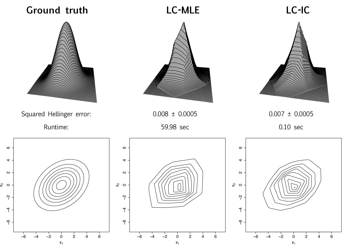
We first demonstrate estimation performance on bivariate normal data, and provide accompanying visualizations of the estimated density. Recalling that , we generate with , and choose the orthogonal matrix at random. With independent samples of generated, we equally split , and compute the LC-IC estimate using PCA to estimate and logcondens to estimate the marginals. From the same samples, we also compute the usual log-concave maximum likelihood estimate (LC-MLE) using the R package LogConcDEAD [12]. Figure 1 shows the ground truth and estimated densities together with their contour plots, and lists the estimation errors in squared Hellinger distance along with the algorithm runtimes. The integrals needed to obtain the squared Hellinger distances are computed via a simple Monte-Carlo procedure (outlined in C.1); the associated uncertainty is also presented in Figure 1.
| LogConICA | 1.27 | 2.87 | 9.17 | 24.92 | 41.64 | |
| LC-IC | 0.02 | 0.01 | 0.02 | 0.04 | 0.06 | |
| LogConICA | 0.38 | 2.99 | 4.01 | 15.99 | 31.35 | |
| LC-IC | 0.02 | 0.03 | 0.05 | 0.09 | 0.10 | |
| LogConICA | 0.44 | 1.49 | 3.22 | 7.60 | 12.33 | |
| LC-IC | 0.02 | 0.04 | 0.10 | 0.12 | 0.18 |
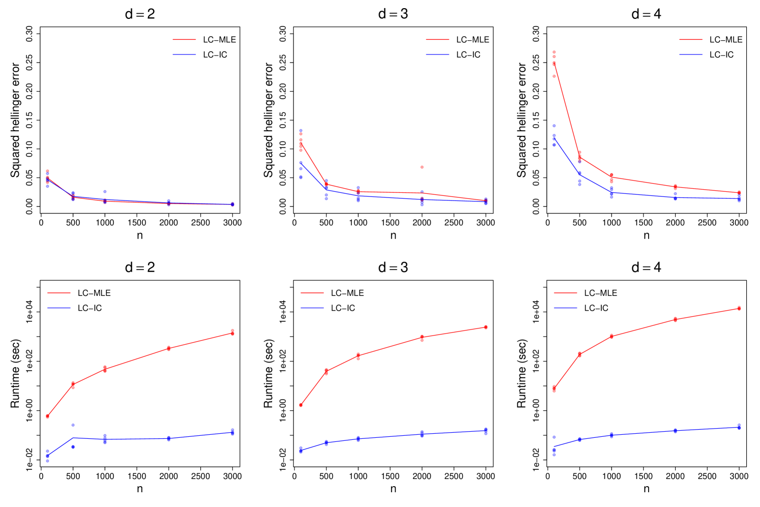
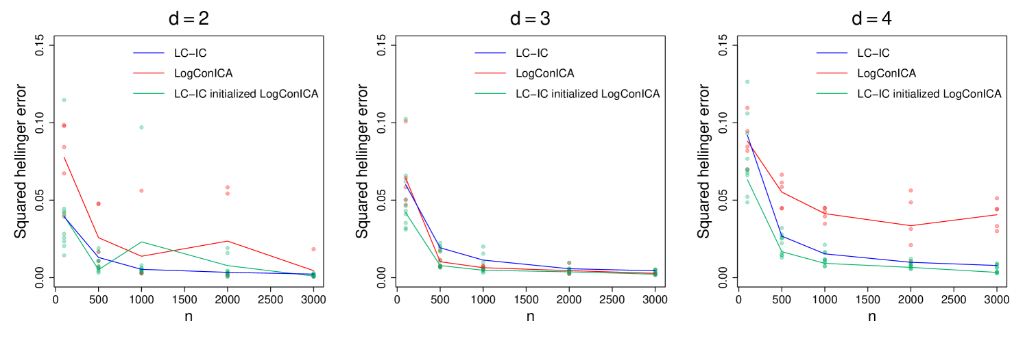
Next, we conduct systematic comparison tests on simulated data from multivariate normal distributions in , with various values of . As before, set with chosen at random and , where for , for , and for . PCA is used for estimating . Each experiment is repeated 5 times and the average metrics are presented. Algorithm runtime comparisons are given in Table 3, whereas the estimation errors in squared Hellinger distance are plotted in Figure 2. Notice that LC-IC runtimes are several orders of magnitude smaller than LC-MLE runtimes, especially for large . Also, the estimation errors of LC-IC are lower than those of LC-MLE, with a growing margin as increases. Similar tests on Gamma-distributed data, are provided in C.3.
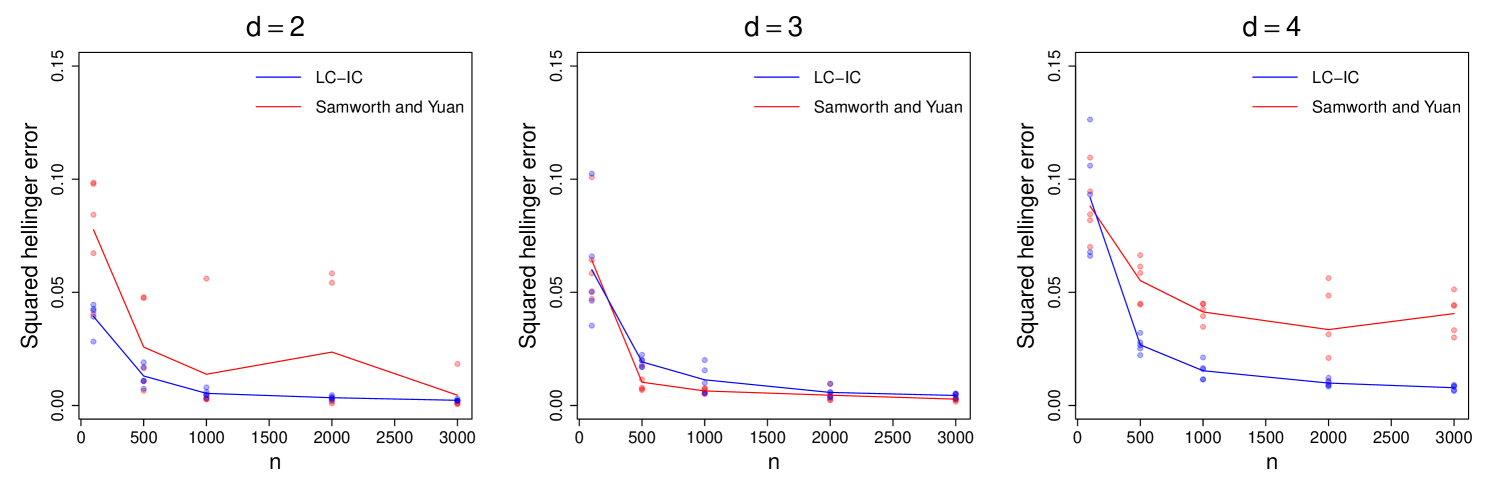
These results are not surprising as the multivariate log-concave MLE is a fully non-parametric procedure that makes no assumptions on except for log-concavity. A fairer comparison is with the LogConICA algorithm of Samworth and Yuan [32]. On simulated data from the uniform distribution with , we compare LC-IC (invoking the kurtosis-based FastICA implementation of ica [20] to estimate , and logcondens to estimate the marginals) with our implementation of LogConICA (using 10 random initializations and a maximum of 20 iterations per initialization). As before, each experiment is repeated 5 times, and the average metrics are presented. Algorithm runtime comparisons are given in Table 4, where we report the average times over the random initializations for LogConICA. The estimation errors in squared Hellinger distance are plotted in Figure 3.
LC-IC still has much shorter runtimes as expected, because it estimates the marginals only once, whereas LogConICA updates those for multiple iterations. Low LogConICA runtimes for larger is peculiar however; this appears to be because the alternating scheme can get stuck quickly at bad points and subsequently terminate. Next, notice that LogConICA can achieve smaller errors than LC-IC (see the plot for ), but may occasionally fail to produce good estimates due to getting stuck at bad points. This could be resolved by better-than-random initialization; one may use our LC-IC estimate as a fast and accurate initial point for LogConICA (see Figure 4).
4.2 Effect of sample splitting proportions
We assess the effect of changing the sample splitting proportions between and on the estimation errors, for multivariate normal data in various dimensions. Using the total number of samples , we define the parameter so that the extreme corresponds to all samples being used for estimating the marginals, and corresponds to all samples being used for estimating .
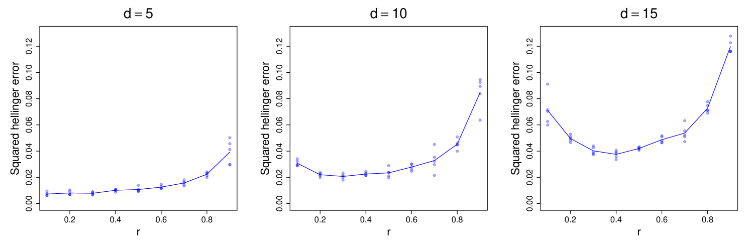
As before, with the orthogonal matrix chosen at random and , where for dimension we set . With total samples, the values are tested. PCA is used for estimating . Each experiment is repeated 5 times independently, and the resulting estimation errors in squared Hellinger distance are presented in Figure 5 for .
Let denote the minimizer of an -versus-error curve for a fixed , and notice that in Figure 5, shifts to the right as increases. This trend is tabulated for all values of tested in Table 5. The observed shift is expected since the bounds for (see Table 2) have a stronger dependence on compared to the bounds for (see Table 1). However, we remark that the effect of has not been completely isolated in the above experiment. The increase in is accompanied by a corresponding decrease in , which worsens the smoothness (or conditioning) of the density. Keeping fixed, on the other hand, would require shrinking the eigengap with .
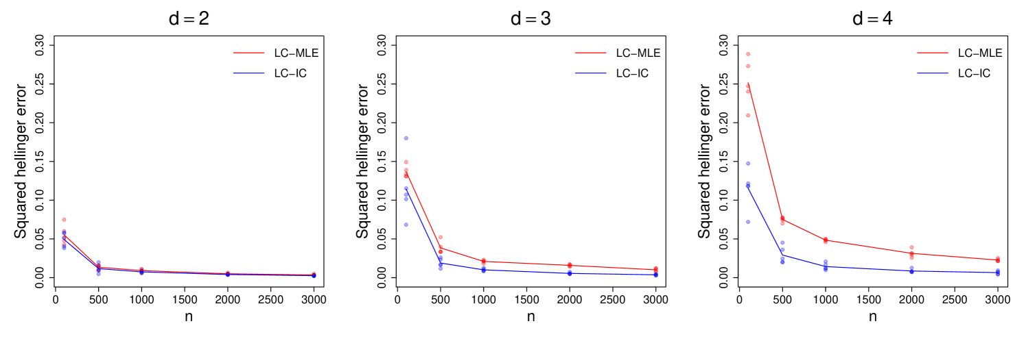
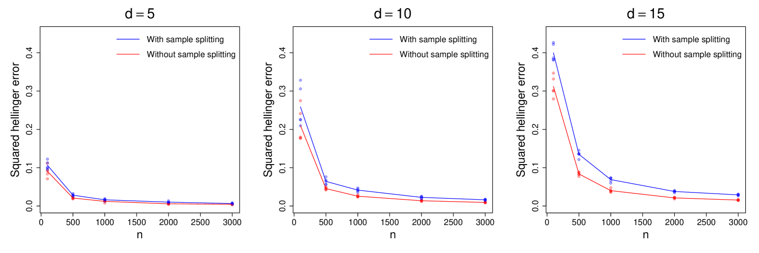
Finally, we test the case of no sample splitting in the setting described above. Here, all samples are used for both marginal estimation and unmixing matrix estimation. We compare the resulting squared Hellinger errors with those of the usual sample splitting variant with , and present the results in Figure 6. We see, somewhat surprisingly, that the variant without sample splitting achieves lower errors. This suggests that any cross-interactions between the marginal and unmixing matrix estimation stages are mild, and both stages benefit from seeing more samples. Our theory from Section 3 does not directly work for this variant without sample splitting, however.
| 2 | 3 | 4 | 5 | 6 | 7 | 8 | 9 | 10 | 15 | |
|---|---|---|---|---|---|---|---|---|---|---|
| 0.1 | 0.1 | 0.1 | 0.1 | 0.2 | 0.2 | 0.3 | 0.3 | 0.3 | 0.4 |
4.3 Estimating mixtures of densities and clustering
Consider the problem of estimating finite mixture densities of the form
| (14) |
where the mixture proportions are nonnegative and sum to 1, and are the component densities corresponding to different clusters. If the component densities are normal, the standard Gaussian EM (expectation maximization) algorithm can be used to estimate . Chang and Walther [9] allowed for the component densities to be univariate log-concave by combining log-concave MLE with the EM algorithm. They also considered a normal copula for the multivariate case. This was later extended to general multivariate log-concave component densities by Cule et al. [11].
Here, we consider mixture densities of the form (14) where the component densities (when centered to mean-zero positions) satisfy the log-concave independent components property. By combining the log-concave independent components estimator (LC-IC) with the EM algorithm, we can port the aforementioned computational benefits to this mixture setting.
We follow the general strategy in Cule et al. [11, Section 6.1], replacing their log-concave MLE step with LC-IC. Such a replacement is not completely obvious however. The log-concave MLE in this setting involves weighted samples, which are not immediately compatible with our sample splitting approach. Instead, we use a re-sampling heuristic as outlined in C.2.
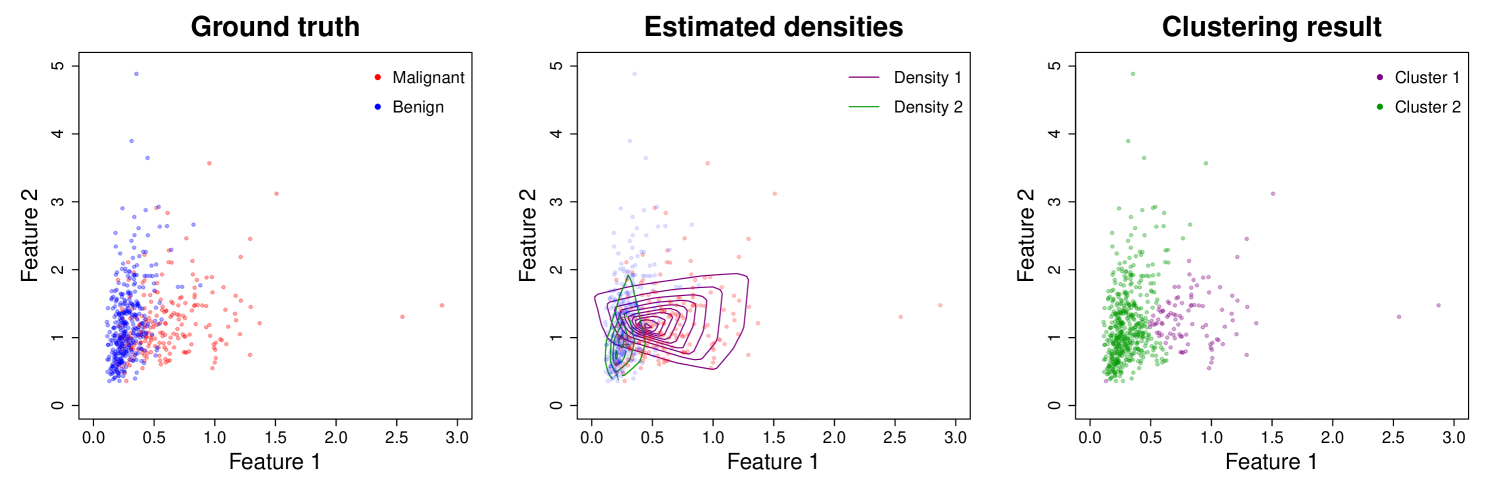
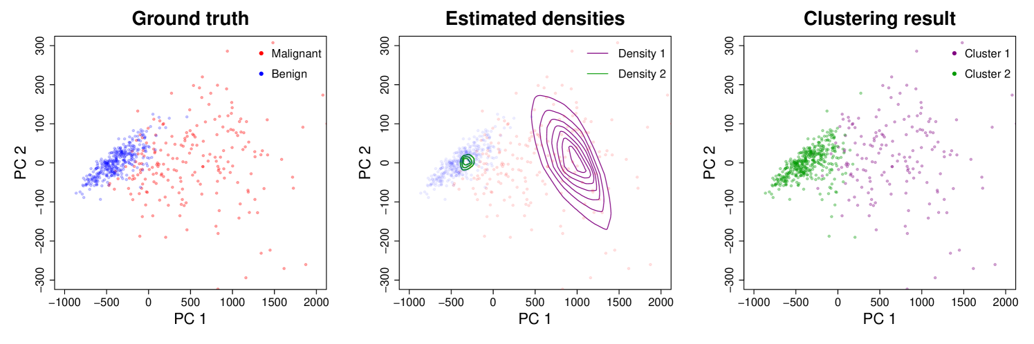
Estimated mixture densities can be used for unsupervised clustering, and we test this on real data. To compare the performance of our EM + LC-IC against the results from Cule et al. [11, Section 6.2], we use the Wisconsin breast cancer dataset [38]. The dataset consists of 569 observations (individuals) and 30 features, where each observation is labeled with a diagnosis of Malignant or Benign. The test involves clustering the data without looking at the labels, and then comparing the learnt clusters with the ground truth labels.
First, we use the same two features as Cule et al. [11]: Feature 1 – standard error of the cell nucleus radius, and Feature 2 – standard error of the cell nucleus texture. This gives bivariate data () with samples. We employ EM + LC-IC with target clusters, random initialization, and 20 EM iterations. Again, PCA is used for the -estimation steps. Figure 7 shows the data with ground truth labels (left-most plot), level curves of the estimated component densities (center plot), and the learnt clusters (right-most plot). Labeling Cluster 1 as Malignant and Cluster 2 as Benign attains a 77.7% classification accuracy (i.e. 77.7% of the instances are correctly labeled by the learnt clusters). This is close to the 78.7% accuracy reported in Cule et al. [11] (121 misclassified instances).
Next, we show improved clustering performance by using more features. Due to the scalability of LC-IC to higher dimensions, one can use all 30 features available in the dataset, so that . We employ EM + LC-IC with target clusters as before, choose an initialization based on agglomerative hierarchical clustering (using the R package mclust [35]), and use 15 EM iterations. The results can be visualized in a PCA subspace of the data – the span of the two leading PCA eigenvectors (or loadings). This particular PCA is only used for visualization, and is separate from the PCA used in estimating .
Figure 8 shows the data in this PCA subspace with ground truth labels (left-most plot), level curves of the estimated component densities (center plot), and the learnt clusters (right-most plot). Labeling Cluster 1 as Malignant and Cluster 2 as Benign achieves an 89.6% classification accuracy, which is a significant improvement over the results for . In comparison, agglomerative hierarchical clustering on its own reaches an accuracy of 86.3%.
5 Discussion
We have looked at statistical and computational aspects of estimating log-concave densities satisfying the orthogonal independent components property. First, we proved that up to iid samples (suppressing constants and log-factors) are sufficient for our proposed estimator to be -close to with high confidence. Although squared Hellinger distance was used here, similar results could have been obtained for total variation (TV) distance since . Note that we do not claim these sample complexity bounds to be tight. The focus here was on demonstrating univariate rates, and a mild dependence on under additional assumptions.
The results here could potentially be processed in the framework of Ashtiani et al. [2], who prove that any family of distributions admitting a so-called sample compression scheme can be learned with few samples. Furthermore, such compressibility extends to products and mixtures of that family. Hence, demonstrating sample compression in our setting would allow extending the sample complexities to mixtures of log-concave independent components densities, providing some theoretical backing to the results from Section 4.3.
Next, the stability results from Section 3.4 could be of further theoretical interest, providing geometric insights into families of densities obtained from orthogonal or linear transformations of product densities. In particular, these could allow one to port covering and bracketing entropies from to higher dimensions by discretizing the operator norm ball in . Also note that these stability bounds are not necessarily tight – consider a spherically symmetric density so that for all orthogonal matrices . Our current analysis does not make use of such symmetry properties.
On the computational side, we showed that our algorithm has significantly smaller runtimes compared to the usual log-concave MLE as well as the LogConICA algorithm of Samworth and Yuan [32]. This was achieved by breaking down the higher dimensional problem into several 1-dimensional ones. In fact these 1-dimensional marginal estimation tasks are decoupled from one another, allowing for effective parallelization to further reduce runtimes. Finally, we demonstrated the scalability of our algorithm by performing density estimation with clustering in .
Acknowledgments
We thank the anonymous referees for several helpful suggestions, and also thank Yaniv Plan for fruitful discussions. Elina Robeva was supported by an NSERC Discovery Grant DGECR-2020-00338.
Parts of this paper were written using the “Latex Exporter” plugin for Obsidian.
References
- Adamczak et al. [2010] Radosław Adamczak, Alexander Litvak, Alain Pajor, and Nicole Tomczak-Jaegermann. Quantitative estimates of the convergence of the empirical covariance matrix in log-concave ensembles. Journal of the American Mathematical Society, 23(2):535–561, 2010.
- Ashtiani et al. [2018] Hassan Ashtiani, Shai Ben-David, Nicholas Harvey, Christopher Liaw, Abbas Mehrabian, and Yaniv Plan. Nearly tight sample complexity bounds for learning mixtures of gaussians via sample compression schemes. Advances in Neural Information Processing Systems, 31, 2018.
- Auddy and Yuan [2023] Arnab Auddy and Ming Yuan. Large dimensional independent component analysis: Statistical optimality and computational tractability. arXiv preprint arXiv:2303.18156, 2023.
- Bagnoli and Bergstrom [2005] Mark Bagnoli and Ted Bergstrom. Log-concave probability and its applications. Economic Theory, 26(2):445–469, 2005.
- Balabdaoui and Wellner [2007] Fadoua Balabdaoui and Jon A Wellner. Estimation of a k-monotone density: Limit distribution theory and the spline connection. The Annals of Statistics, 35(6):2536–2564, 2007.
- Barber and Samworth [2021] Rina Foygel Barber and Richard J Samworth. Local continuity of log-concave projection, with applications to estimation under model misspecification. Bernoulli, 27(4):2437–2472, 2021.
- Carpenter et al. [2018] Timothy Carpenter, Ilias Diakonikolas, Anastasios Sidiropoulos, and Alistair Stewart. Near-optimal sample complexity bounds for maximum likelihood estimation of multivariate log-concave densities. In Conference On Learning Theory, pages 1234–1262. PMLR, 2018.
- Chae and Walker [2020] Minwoo Chae and Stephen G. Walker. Wasserstein upper bounds of the total variation for smooth densities. Statistics & Probability Letters, 163:108771, 2020. ISSN 0167-7152.
- Chang and Walther [2007] George T Chang and Guenther Walther. Clustering with mixtures of log-concave distributions. Computational Statistics & Data Analysis, 51(12):6242–6251, 2007.
- Comon and Jutten [2010] Pierre Comon and Christian Jutten. Handbook of Blind Source Separation: Independent component analysis and applications. Academic press, 2010.
- Cule et al. [2010] Madeleine Cule, Richard Samworth, and Michael Stewart. Maximum likelihood estimation of a multi-dimensional log-concave density. Journal of the Royal Statistical Society: Series B (Statistical Methodology), 72(5):545–607, 2010.
- Cule et al. [2023] Madeleine Cule, Robert Gramacy, Richard Samworth, and Yining Chen. LogConcDEAD: Log-Concave Density Estimation in Arbitrary Dimensions, 2023. URL https://CRAN.R-project.org/package=LogConcDEAD. R package version 1.6-8.
- Dempster et al. [1977] Arthur P Dempster, Nan M Laird, and Donald B Rubin. Maximum likelihood from incomplete data via the em algorithm. Journal of the royal statistical society: series B (methodological), 39(1):1–22, 1977.
- Doss and Wellner [2016] Charles R Doss and Jon A Wellner. Global rates of convergence of the MLEs of log-concave and s-concave densities. The Annals of Statistics, 44(3):954, 2016.
- Dümbgen et al. [2011] Lutz Dümbgen, Richard Samworth, and Dominic Schuhmacher. Approximation by log-concave distributions, with applications to regression. Annals of statistics, 39(2):702–730, 2011.
- Gibbs and Su [2002] Alison L Gibbs and Francis Edward Su. On choosing and bounding probability metrics. International statistical review, 70(3):419–435, 2002.
- Goyal et al. [2014] Navin Goyal, Santosh Vempala, and Ying Xiao. Fourier pca and robust tensor decomposition. In Proceedings of the Forty-Sixth Annual ACM Symposium on Theory of Computing, STOC ’14, page 584–593, New York, NY, USA, 2014. Association for Computing Machinery. ISBN 9781450327107.
- Grenander [1956] Ulf Grenander. On the theory of mortality measurement: Part ii. Scandinavian Actuarial Journal, 1956(2):125–153, 1956.
- Groeneboom et al. [2001] Piet Groeneboom, Geurt Jongbloed, and Jon A Wellner. Estimation of a convex function: Characterizations and asymptotic theory. The Annals of Statistics, 29(6):1653–1698, 2001.
- Helwig [2022] Nathaniel E. Helwig. ica: Independent Component Analysis, 2022. URL https://CRAN.R-project.org/package=ica. R package version 1.0-3.
- Holmström and Klemelä [1992] Lasse Holmström and Jussi Klemelä. Asymptotic bounds for the expected l1 error of a multivariate kernel density estimator. Journal of multivariate analysis, 42(2):245–266, 1992.
- Hyvärinen and Oja [2000] Aapo Hyvärinen and Erkki Oja. Independent component analysis: algorithms and applications. Neural networks, 13(4-5):411–430, 2000.
- Kim et al. [2018] Arlene K. Kim, Adityanand Guntuboyina, and Richard J. Samworth. Adaptation in log-concave density estimation. The Annals of Statistics, 46(5):2279 – 2306, 2018. 10.1214/17-AOS1619.
- Kim and Samworth [2016] Arlene KH Kim and Richard J Samworth. Global rates of convergence in log-concave density estimation. The Annals of Statistics, 44(6):2756–2779, 2016.
- Koenker and Mizera [2010] Roger Koenker and Ivan Mizera. Quasi-concave density estimation. The Annals of Statistics, 38(5):2998–3027, 2010.
- Kubjas et al. [2022] Kaie Kubjas, Olga Kuznetsova, Elina Robeva, Pardis Semnani, and Luca Sodomaco. Log-concave density estimation in undirected graphical models. arXiv preprint arXiv:2206.05227, 2022.
- Kur et al. [2019] Gil Kur, Yuval Dagan, and Alexander Rakhlin. Optimality of maximum likelihood for log-concave density estimation and bounded convex regression. arXiv:1903.05315, 2019.
- Lovász and Vempala [2007] László Lovász and Santosh Vempala. The geometry of logconcave functions and sampling algorithms. Random Structures & Algorithms, 30(3):307–358, 2007. https://doi.org/10.1002/rsa.20135.
- Meyers and Serrin [1964] Norman G. Meyers and James Serrin. H = W. Proceedings of the National Academy of Sciences, 51(6):1055–1056, 1964. 10.1073/pnas.51.6.1055.
- Robeva et al. [2021] Elina Robeva, Bernd Sturmfels, Ngoc Tran, and Caroline Uhler. Maximum likelihood estimation for totally positive log-concave densities. Scandinavian Journal of Statistics, 48(3):817–844, 2021.
- Rufibach and Duembgen [2023] Kaspar Rufibach and Lutz Duembgen. logcondens: Estimate a Log-Concave Probability Density from Iid Observations, 2023. URL https://CRAN.R-project.org/package=logcondens. R package version 2.1.8.
- Samworth and Yuan [2012] Richard Samworth and Ming Yuan. Independent component analysis via nonparametric maximum likelihood estimation. The Annals of Statistics, 40(6):2973 – 3002, 2012. 10.1214/12-AOS1060.
- Samworth [2018] Richard J. Samworth. Recent Progress in Log-Concave Density Estimation. Statistical Science, 33(4):493 – 509, 2018. 10.1214/18-STS666. URL https://doi.org/10.1214/18-STS666.
- Schuhmacher and Dümbgen [2010] Dominic Schuhmacher and Lutz Dümbgen. Consistency of multivariate log-concave density estimators. Statistics & probability letters, 80(5-6):376–380, 2010.
- Scrucca et al. [2023] Luca Scrucca, Chris Fraley, T. Brendan Murphy, and Adrian E. Raftery. Model-Based Clustering, Classification, and Density Estimation Using mclust in R. Chapman and Hall/CRC, 2023. ISBN 978-1032234953. 10.1201/9781003277965. URL https://mclust-org.github.io/book/.
- Vershynin [2018] Roman Vershynin. High-dimensional probability: An introduction with applications in data science, volume 47. Cambridge university press, 2018.
- Walther [2002] Guenther Walther. Detecting the presence of mixing with multiscale maximum likelihood. Journal of the American Statistical Association, 97(458):508–513, 2002.
- Wolberg et al. [1995] William Wolberg, Olvi Mangasarian, Nick Street, and W. Street. Breast Cancer Wisconsin (Diagnostic). UCI Machine Learning Repository, 1995. DOI: https://doi.org/10.24432/C5DW2B.
- Xu and Samworth [2021] Min Xu and Richard J. Samworth. High-dimensional nonparametric density estimation via symmetry and shape constraints. The Annals of Statistics, 49(2):650 – 672, 2021. 10.1214/20-AOS1972. URL https://doi.org/10.1214/20-AOS1972.
- Yu et al. [2015] Yi Yu, Tengyao Wang, and Richard J Samworth. A useful variant of the davis–kahan theorem for statisticians. Biometrika, 102(2):315–323, 2015.
Appendix A Delayed proofs
Here, we present the proofs that were deferred in the main text. We will need some additional notation. Let be the set of probability distributions on satisfying and for every hyperplane . The log-concave projection of Dümbgen et al. [15] is a map from to the set of log-concave densities on , defined by
Also define, given the minimal first moment
A.1 Proof of Theorem 3.5
We recall the statement below.
Statement
Suppose is a zero-mean probability density on , satisfying the orthogonal independent components property with independent directions . Let be the proposed estimator (Definition 2.4). We have the error bound
where .
Proof A.1.
For , denote the projection . This allows us to write the proposed estimator as
| (15) |
We can break down into three terms that need to be controlled:
| (16) |
This is essentially removing hats one-at-a-time. The first term is handled as
| (17) |
using the simple tensorization argument from Lemma 3.1. Since , which is the density of , we get that the third term equals .
Finally, consider the second term. Noting that and using Lemma B.1 gives
| (18) |
Now, to bound the second term, note that
via the change of variables . The above expression can be lower bounded using (18):
where the last bound follows from Bernoulli’s inequality. Hence,
which completes the last bit of the proof of Theorem 3.5.
A.2 Proof of Lemma 3.6
We recall the statement below.
Statement
Let be a zero-mean log-concave density on , and let be any invertible matrix. Then,
where is the covariance matrix of , and the constant depends only on the dimension .
Proof A.2.
We will use properties of the log-concave projection . Firstly, is a log-concave density by assumption, and by the linearity and invertibility of , so is . As a result, and . By Theorem 2 of Barber and Samworth [6],
where is a constant that depends only on . We will conclude by upper-bounding the Wasserstein-1 distance and lower bounding .
A.3 Proof of Theorem 3.8
We recall the statement below.
Statement (brief)
Let be a zero-mean log-concave density on satisfying the orthogonal independent components property, and let be the proposed estimator. Then, for any and , we have
with probability at least whenever
| (19) | |||
| and | |||
Proof A.3.
By Theorem 3.5, decompose as
where . We show that holds with probability at least when is large enough, and that holds with probability at least when is large enough. A final union bound then gives the desired result.
We handle first. Write and , and denote the marginal error for to highlight the dependence on and . Then, one can use the independence of and to express, for any ,
where denotes the indicator of an event, and , denote expectation with respect to the distributions of and respectively. As a result, it suffices to bound for any deterministic .
Recall that the estimated independent directions are computed from the samples in . For a deterministic , the corresponding are deterministic as well. In this case, the projected samples are independent and identically distributed with law , and as a result,
holds for provided . Now, re-introducing the randomness in and taking expectation gives . We set and , and use a union bound over to finally get
A.4 Proof of Proposition 3.9
We recall the statement below.
Statement
Let be a univariate log-concave density, and denote by the log-concave MLE computed from iid samples from . Given and , we have
with probability at least whenever
for absolute constants .
Proof A.4.
Lemma 6 and the proof of Theorem 5 of Kim and Samworth [24] imply the concentration bound
for suitably large absolute constants . Setting in the concentration bound gives that
Now, holds provided , and holds provided . Setting , and concludes the proof.
A.5 Proof of Proposition 3.11
We recall the statement below.
Statement
Let be a univariate log-concave density, and fix . Denote by the boosted log-concave MLE at error threshold , computed from independent batches of iid samples from each. Given , we have
with probability at provided
for absolute constants .
Proof A.5.
We follow the proof of Theorem 2.8 of Lovász and Vempala [28]. Firstly, for a sufficiently large ensures (by Markov’s inequality) that
for each batch . Then, by Chernoff’s inequality, strictly more than ()-many batches satisfy simultaneously, with probability at least . Under this event, suppose is returned. Then there exists some such that and , so that by triangle inequality, . Finally, choosing makes the probability of this event .
A.6 Proof of Proposition 3.12
We recall the statement below.
Statement
(Sample complexity of estimating by PCA). Let be a zero-mean, log-concave probability density on . Let be samples, and suppose Moment assumption M1 is satisfied with eigenvalue separation . Let and , and define . If
then with probability at least , PCA recovers vectors such that
up to permutations and sign-flips.
Proof A.6.
Since and are eigenvectors of and respectively, the Davis-Kahan theorem (see Yu et al. [40], or Theorem 4.5.5 of Vershynin [36]) gives the bound
for some permutation and choice of sign-flips of . Hence, the problem boils down to covariance estimation of log-concave random vectors [1].
To bring the problem into an isotropic setting, define random vectors for , such that , and note that these still have log-concave densities. Let be absolute constants. By Theorem 4.1 of Adamczak et al. [1], for any and , if
then with probability at least , it holds that
| (20) |
For a , we have so that setting for a large enough absolute constant results in the failure probability being bounded above as . Hence, (20) holds with probability at least , provided
Furthermore, letting yields that
with probability at least provided . As a result, (20) also extends to . Finally, letting and adjusting the absolute constants gives the required result, since
A.7 Proof of Proposition 3.13
We recall the statement below.
Statement
Let be a zero-mean probability density on satisfying the orthogonal independent components property. Suppose, additionally, that Moment assumption M2 is satisfied with parameters and . Given and , and samples , if
for constants depending on , then with probability at least , ICA recovers vectors such that
for independent directions of .
Proof A.7.
Given vectors , Auddy and Yuan [3] consider discrepancy in their bounds. We can relate this to the distance up to a sign-flip. More precisely, pick a such that . In this case,
Next, the algorithm of Auddy and Yuan [3] produces vectors which estimate the columns of . Recall that the columns of are simply scalings of independent directions . Rescaling as does not change the angles, and hence,
(flipping the sign of as required). To get orthonormal estimates , we form a matrix with columns , compute the singular value decomposition and set , which is the closest orthogonal matrix to in Frobenius norm. As a result,
Finally, we required a bound on the 9th moment of in Moment assumption M2, instead of on some th moment, for the sake of simplicity. Using these facts, and setting in Theorem 3.4 of Auddy and Yuan [3] to , gives the desired form of the result.
A.8 Proof of Lemma 3.14
We recall the statement below.
Statement
Let be a zero-mean probability density on , satisfying Smoothness assumption S1. Let be any orthogonal matrix. Then,
Proof A.8.
Recall that . The KL divergence
| (21) |
where . Since KL is always non-negative, an upper bound suffices to show closeness between and .
Using smoothness assumption S1 i.e. with , we get a Taylor-like expansion
| (22) |
for . Setting , and plugging (22) into (21) yields
| (23) |
The second term can be handled as
since .
Now consider the first term in (23). Note that , and as a result,
is finite by the integrability conditions in Smoothness assumption S1. We use integration by parts, and write
where is the Euclidean ball of radius centered at the origin, is the outward normal vector field on , and is the -dimensional surface area measure. We claim that the boundary term is zero; to see this, define
for , and note that controls the boundary term as
It follows from the integrability conditions in Smoothness assumption S1 that and its derivative are integrable on , and as a consequence, (see Lemma B.9 for details).
Hence,
But note that for any orthogonal ,
where are the standard basis vectors in . We conclude that the the first term in (23) is non-positive, and put these bounds together with to get the desired result.
A.9 Proof of Lemma 3.15
We recall the statement below.
Statement
Let be a zero-mean probability density on , satisfying Smoothness assumption S2. Let be invertible with . Then,
Proof A.9.
Let be the transformed density. Consider the standard Gaussian density on , and for any (to be fixed later), denote the scaled version by . We can decompose
| (24) |
To bound the second term of (24), we use Lemma B.11 and Lemma B.13, and get
| (25) |
The right-hand side is now a problem of stability in the Wasserstein-1 distance, and is handled by Lemma B.7. Noting that , Lemma B.7 together with (25) give the bound
which concludes the analysis of the second term of (24). Now, we handle the first and third terms of (24), making use of the assumed smoothness (S2) of .
Lemma B.15 directly bounds the third term of (24). To address the first term, we apply Lemma B.15 to , noting that . This finally yields the bound
The following choice completes the proof of Lemma 3.15.
A.10 Proof of Corollary 3.16
We recall the statement below.
Statement (brief)
Let be a zero-mean probability density on , satisfying the orthogonal independent components property, and let be the proposed estimator. Then, for any and , we have
with probability at least whenever
| (26) | |||
| and | |||
Proof A.10.
The inequality for is the same as in Theorem 3.8, and follows the same argument (see A.3). Now consider the inequalities for . Suppose Smoothness assumption S1 holds. Then,
and similarly for . For any , note that samples are sufficient to give
with probability at least . Setting
then gives
as desired. Now, if Smoothness assumption S2 holds, then
As before, we consider and note that samples are sufficient to give
with probability at least . Setting
concludes the proof.
A.11 Proof of Theorem 3.18
We recall the statement below.
Statement
Let be a zero-mean distribution in , satisfying the orthogonal independent components property with independent directions . Let be the proposed estimator computed from samples . We have the error bound
where .
Proof A.11.
Since satisfies the orthogonal independent components property with independent directions , it follows from Theorem 2 of Samworth and Yuan [32] that the density factorizes as
Similar to the proof of Theorem 3.5, we then decompose
By the tensorization argument of Lemma 3.1,
An identical calculation also yields
Finally, noting that , we can rewrite
Since the log-concave projection commutes with affine maps [15], we have that which concludes the proof.
A.12 Proof of Theorem 3.19
We recall the statement below.
Statement (brief)
Let be a zero-mean distribution in satisfying the orthogonal independent components property. Suppose that Moment assumption M2 is satisfied, , and for some . Let be the proposed estimator, invoking log-concave MLE and ICA. Then, for any and , we have
with probability at least whenever
and
Proof A.12.
The proof follows the same pattern as that of Theorem 3.8. We use the error bound from Theorem 3.18:
First, we show that holds with probability at least , provided is large enough. By a conditioning argument on as before, we can treat as deterministic for this part of the proof.
Define the empirical distribution , and denote it’s -marginal by for . Since we used log-concave MLE to estimate the marginals in this setting, we can express . Noting that is itself an empirical distribution of for each , Theorem 5 of Barber and Samworth [6] gives the bound
for a constant depending only on . (In applying the theorem, we have used the simple facts that and for all ). A direct application of Markov’s inequality also gives the tail bound
for any . The right-hand side is bounded above by some provided
We set and , and use a union bound over to finally get
Now consider term (II). By Theorem 2 of Barber and Samworth [6], we have that
for an absolute constant , where one can further simplify
Theorem 2 of Barber and Samworth [6] can also be used to bound term (III) as
where depends only on , and we note that
Putting these inequalities together gives
for some depending only on . Applying Proposition 3.13 allows us to conclude that with probability at least provided
for a suitably chosen depending only on .
Appendix B Auxiliary lemmas
Here, we prove the various lemmas invoked in Appendix A.
Lemma B.1.
Let , where each is a univariate probability density, and consider any other probability density . Then,
for .
The above lemma bounds the 1-dimensional Hellinger distance between marginals by the -dimensional Hellinger distance between the full densities. This is a special case of the data processing inequality for -divergences, but we nevertheless provide a proof below.
Proof B.2.
Writing
and changing variables gives
where . Splitting the components of as and allows us to rewrite the above expression as an iterated integral, and use Cauchy-Schwarz on the inner integral:
Since each is a probability density,
On the other hand, is being marginalized and
is the marginal of along the direction . Noting that and chaining together the above inequalities gives the desired result:
Lemma B.3 (Jensen gap for univariate log-concave densities).
Let be any univariate log-concave probability density, and suppose . Then,
holds for .
Proof B.4.
Define the ‘standardized’ random variable where and are the mean and standard deviation of respectively. Denote the density of by , and note that is an isotropic log-concave density. By Theorem 5.14(a) of Lovász and Vempala [28] specialized to the case , we have the lower bound for , which can be used to estimate
Additionally, by Lemma 5.5(b) of Lovász and Vempala [28], . We conclude that for , which can be transformed to give
The upper bound on is immediate from Jensen’s inequality or the Cauchy-Schwarz inequality.
Lemma B.5 (lower bound on for a log-concave density).
Let be any log-concave density on , with mean and covariance matrix . Then,
holds for .
Proof B.6.
Let (which exists by compactness and continuity). For , note that has a univariate log-concave density , so that one can apply Lemma B.3 to conclude that
Lemma B.7 (Stability in ).
Let be a probability density on with mean zero and covariance matrix , and let . Then,
Proof B.8.
A direct calculation yields
The result then follows because .
Lemma B.9 (Controlling the boundary integral).
Let be a continuously differentiable probability density on , such that and . Then, the function
is differentiable on , and moreover, and are integrable on . Consequently, we also have that .
Proof B.10.
Using spherical integration, we immediately get that
To get , we differentiate under the integral sign as
which is justified because the differentiated integrand is continuous in , and as a result, can be uniformly bounded in magnitude by a constant over all and all in any compact subset of . Now, integrating gives
What remains, finally, is to show that . The integrability of implies that the limit
exists finitely. But if were a non-zero number, then would not be integrable over , leading to a contradiction. Hence, we may conclude that as required.
For the next few lemmas, recall that and .
Lemma B.11 ( bound on smoothed densities).
Let and be probability densities on , and denote by the Wasserstein-1 distance between them. For any , it holds that
where denotes a translation for any function on .
Proof B.12.
Denote by the set of all couplings (or transport plans) between and , and let . Note that one can express
A direct calculation involving an exchange of integrals and a Holder bound gives
Taking an infimum over all gives the desired result.
Lemma B.13 (Translational stability of Gaussian kernels in ).
Let , and . Then,
Proof B.14.
Fix some and consider the smooth function where linearly interpolates between and . This lets us write
Integrating, we get that
What remains is to bound the integral , and this is straightforward. Noting that
we get
which completes the proof of the lemma.
Lemma B.15 ( error due to mollification).
Proof B.16.
We first relate the approximation error above to the translational stability in :
This translational stability is controlled via smoothness. Suppose first that , so that for ,
Integrating gives
If , one can use the fact that lives in the Sobolev space to get an approximating sequence satisfying and [29]. This allows us to extend the bound
to all . Combining, we get
Appendix C Computational details and further numerical results
C.1 Monte Carlo integration for computing squared Hellinger distances
Recall that the squared Hellinger between densities and on is defined by the integral
| (27) |
If is larger than 4, computing the integral by discretizing on a grid can prove prohibitively expensive. Instead, one can use simple Monte Carlo integration to approximate (27). Notice that
where the expectation on the right-hand side can be approximated using an empirical average. We simulate samples , and compute
which converges almost surely to as . In practice, we use . Additionally, we repeat the procedure 50 times and ensure that the resulting spread is not too large.
C.2 The EM algorithm and the re-sampling heuristic
Recall the finite mixture densities discussed in Section 4.3
and consider samples . We briefly describe the EM algorithm following Cule et al. [11]. Given current iterates of the mixture proportions and component densities , compute the posterior probabilities
| (28) |
Then, for each component , update the density by maximizing a weighted likelihood over a suitable class of densities (such as log-concave densities):
| (29) |
Finally, update the mixture proportions as
| (30) |
for each . These three step can be iterated until convergence.
When combining the EM algorithm with LC-IC, (28) and (30) remain unchanged. Only the maximum likelihood step (29) needs to be replaced, where one needs to “fit” a density to samples weighted by . Since weighted samples are not immediately compatible with our sample splitting scheme, we propose the following heuristic re-sampling scheme. From the observed samples , construct the weighted empirical distribution
for each . Notice that depends on the current iterates. Next, (computationally) generate iid samples from (hence the term re-sampled), and feed them into Algorithm 1, using of those re-sampled samples for the unmixing matrix estimation stage, and for the marginal estimation stage. The output of Algorithm 1 is then the updated iterate of . Unlike the sample splitting scheme discussed before, the re-sampling heuristic involves no compromise between and ; one can generate as many samples from as they like. The experiments in Section 4.3 used .
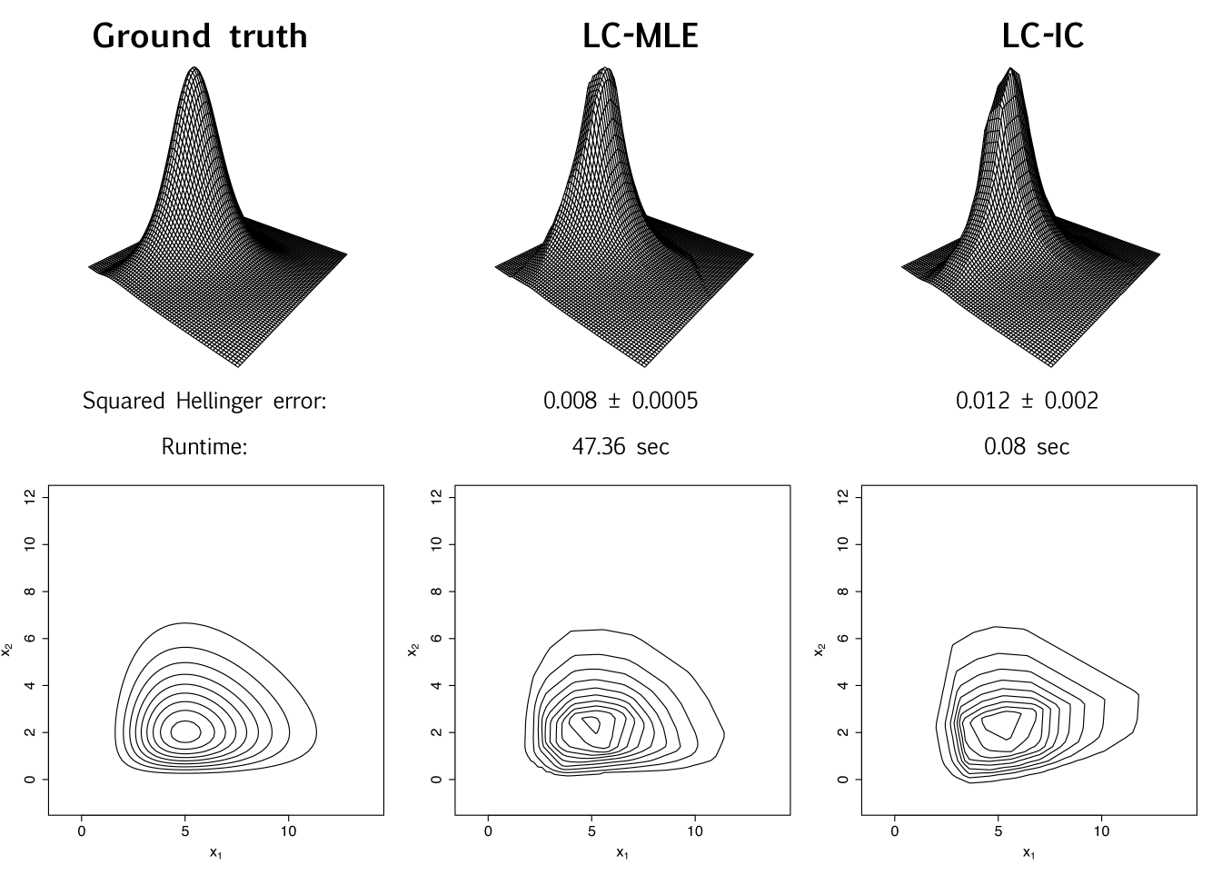
However, it is important to note that we do not have a theoretical backing for this heuristic yet. Another issue in this strategy is the generation of spuriously zeros values of , which can cause division-by-zero errors and likelihoods of . We address this by adding a small positive number such as to the zero values of .
C.3 Comparison of performance on Gamma-distributed data
Here, we repeat the experiments from Section 4.1, but for Gamma distributed data. Consider the bivariate case first. Let with and , such that and . With iid samples of generated, equally split , and compute the LC-IC estimate using PCA for unmixing matrix estimation and logcondens for marginal estimation. From the same samples, also compute the LC-MLE estimate with LogConcDEAD. Figure 9 shows the ground truth and estimated densities together with their contour plots, and lists the estimation errors in squared Hellinger distance along with the algorithm runtimes.
Then, we conduct systematic tests similar to Section 4.1 for and various . Set , where and , with . PCA is used for estimating . Each experiment is repeated 5 times, and the average metrics are computed. Figure 10 plots the estimation errors in squared Hellinger distance, as well as the algorithm runtimes, for both LC-MLE and LC-IC. The results are consistent with those from Section 4.1.