Log-Concavity of the Genus Polynomials of Ringel Ladders

Our graphs are implicitly taken to be connected, and our graph embeddings are cellular and orientable. For general background in topological graph theory, see [13, 1]. Prior acquaintance with the concepts of partitioned genus distribution (abbreviated here as pgd) and production (e.g., [10, 17]) are necessary preparation for reading this paper. The exposition here is otherwise intended to be accessible both to graph theorists and to combinatorialists.

The number of combinatorially distinct embeddings of a graph $G$ in the orientable surface of genus $i$ is denoted by $g_{i}(G)$. The sequence $g_{0}(G)$, $g_{1}(G)$, $g_{2}(G)$, $\ldots$, is called the genus distribution of $G$. A genus distribution contains only finitely many positive numbers, and there are no zeros between the first and last positive numbers. The genus polynomial is the polynomial

Log-concave sequences

A sequence $A=(a_{k})_{k=0}^{n}$ is said to be nonnegative, if $a_{k}\geq 0$ for all $k$. An element $a_{k}$ is said to be an internal zero of $A$ if $a_{k}=0$ and if there exist indices $i$ and $j$ with $i<k<j$, such that $a_{i}a_{j}\neq 0$. If $a_{k-1}a_{k+1}\leq a_{k}^{2}$ for all $k$, then $A$ is said to be log-concave. If there exists an index $h$ with $0\leq h\leq n$ such that

then $A$ is said to be unimodal. It is well-known that any nonnegative log-concave sequence without internal zeros is unimodal, and that any nonnegative unimodal sequence has no internal zeros. A prior paper [11] by the present authors provides additional contextual information regarding log-concavity and genus distributions.

For convenience, we sometimes abbreviate the phrase “log-concave genus distribution” as LCGD. Proofs that closed-end ladders and doubled paths have LCGDs [4] were based on explicit formulas for their genus distributions. Proof that bouquets have LCGDs [12] was based on a recursion. A conjecture that all graphs have LCGDs was published by [12].

Stahl’s method [21, 22] of representing what we have elsewhere formulated as simultaneous recurrences [4] or as a transposition of a production system for a surgical operation on graph embeddings as a matrix of polynomials can simplify a proof that a family of graphs has log-concave genus distributions, without having to derive the genus distribution itself.

Newton’s theorem that real-rooted polynomials with non-negative coefficients are log-concave is one way of getting log-concavity. Stahl [22] made the general conjecture (Conjecture 6.4) that all genus polynomials are real-rooted, and he gave a collection of specific test families. Shortly thereafter, Wagner [24] proved that the genus distributions for the related closed-end ladders and various other test families suggested by [22] are real-rooted. However, Liu and Wang [16] answered Stahl’s general conjecture in the negative, by exhibiting a chain of copies of the wheel graph $W_{4}$, one of Stahl’s test families, that is not real-rooted. Our previous paper [11] proves, nonetheless, that the genus distribution of every graph in the $W_{4}$-linear sequence is log-concave. Thus, even though Stahl’s proposed approach to log-concavity via roots of genus polynomials is sometimes infeasible, results in [11] do support Stahl’s expectation that chains of copies of a graph are a relatively accessible aspect of the general LCGD problem. The genus distributions for the family of Ringel ladders, whose log-concavity is proved in this paper, are not real-rooted either.

Log-concavity of genus distributions for directed graph embeddings has been studied by [2] and [3]. Another related area is the continuing study of maximum genus of graphs, of which [15] is an example.

Linear, ringlike, and tree-like families

Stahl used the term“$H$-linear” to describe chains of graphs that are constructed by amalgamating copies of a fixed graph $H$. Such amalgamations are typically on a pair of vertices, one in each of the amalgamands, or on a pair of edges. It seems reasonable to generalize the usage of linear in several ways, for instance, by allowing graphs in the chain to be selected from a finite set.

We use the term ring-like to describe a graph that results from any of the following topological operations on a doubly rooted linear chain with one root in the first graph of the chain and one in the last graph:

1. (1)

   a self-amalgamation of two root-vertices;

2. (2)

   a self-amalgamation of two root-edges;

3. (3)

   joining one root-vertex to the other root-vertex (which is called a self-bar-amalgamation).

Every graph can be regarded as tree-like in the sense of tree decompositions. However, we use this term only when a graph is not linear or ring-like. For any fixed tree-width $w$ and fixed maximum degree $\Delta$, there is a quadratic-time algorithm [8] to calculate the genus polynomial of graphs of parameters $w$ and $\Delta$. One plausible approach to the general LCGD conjecture might be to prove it for fixed tree-width and fixed maximum degree. Recurrences have been given for the the genus distributions of cubic outerplanar graphs [6], 4-regular outerplanar graphs [18], and cubic Halin graphs [7], all three of which are tree-like. However, none of these genus distributions have been proved to be log-concave. Nor have any other tree-like graphs been proved to have LCGDs.

This paper is organized as follows. Section 2 describes a representation of partitioning of the genus distribution into ten parts as a pgd-vector. Section 3 describes how productions are used to describe the effect of a graph operation on the pgd-vector. Section 4 analyzes how self-bar amalgamation affects the genus distribution. Section 5 offers a new derivation of the genus distributions of the Ringel ladders and proof that these genus distributions are log-concave.

A fundamental strategy in the calculation of genus distributions, from the outset [4], has been to partition a genus distribution according to the incidence of face-boundary walks on one or more roots. We abbreviate “face-boundary walk” as fb-walk. For a graph $(G,u,s)$ with two 2-valent root-vertices, we can partition the number $g_{i}(G)$ into the following four parts:

$dd_{i}(G)$:

the number of embeddings of $(G,u,v)$ in the surface $S_{i}$ such that two distinct fb-walks are incident on root $u$ and two on root $v$;

$ds_{i}(G)$:

the number of embeddings in $S_{i}$ such that two distinct fb-walks are incident on root $u$ and only one on root $v$;

$sd_{i}(G)$:

the number of embeddings in $S_{i}$ such that one fb-walk is twice incident on root $u$ and two distinct fb-walks are incident on root $v$;

$ss_{i}(G)$:

the number of embeddings in $S_{i}$ such that one fb-walk is twice incident on root $u$ and one is twice incident on root $v$.

$dd^{0}_{i}(G)$:

the number of type-$dd$ embeddings of $(G,u,v)$ in $S_{i}$ such that neither fb-walk incident at root $u$ is incident at root $v$;

$dd^{\prime}_{i}(G)$:

the number of type-$dd$ embeddings in $S_{i}$ such that one fb-walk incident at root $u$ is incident at root $v$;

$dd^{\prime\prime}_{i}(G)$:

the number of type-$dd$ embeddings in $S_{i}$ such that both fb-walks incident at root $u$ are incident at root $v$;

$ds^{0}_{i}(G)$:

the number of type-$ds$ embeddings in $S_{i}$ such that neither fb-walk incident at root $u$ is incident at root $v$;

$ds^{\prime}_{i}(G)$:

the number of type-$ds$ embeddings in $S_{i}$ such that one fb-walk incident at root $u$ is incident at root $v$;

$sd^{0}_{i}(G)$:

the number of type-$sd$ embeddings in $S_{i}$ such that the fb-walk incident at root $u$ is not incident on root $v$;

$sd^{\prime}_{i}(G)$:

the number of type-$sd$ embeddings in $S_{i}$ such that the fb-walk at root $u$ is also incident at root $v$;

$ss^{0}_{i}(G)$:

the number of type-$ss$ embeddings in $S_{i}$ such that the fb-walk incident at root $u$ is not incident on root $v$;

$ss^{1}_{i}(G)$:

the number of type-$ss$ embeddings in $S_{i}$ such that the fb-walk incident at root $u$ is incident at root $v$, and the incident pattern is $uuvv$;

$ss^{2}_{i}(G)$:

the number of type-$ss$ embeddings in $S_{i}$ such that the fb-walk incident at root $u$ is incident at root $v$, and the incident pattern is $uvuv$.

We define the symmetric ladder $(\ddot{L}_{n},u,v)$ to be the graph obtained from the cartesian product $P_{2}\Box P_{n+2}$ by contracting the respective edges at both ends that join a pair of 2-valent vertices and designating the remaining two 2-valent vertices at the ends of the ladder as root-vertices. The symmetric ladders $(\ddot{L}_{1},u,v)$ and $(\ddot{L}_{2},u,v)$ are illustrated in Figure 3.1. The location of the roots of a symmetric ladder at opposite ends causes it to have a different partitioned genus distribution from other ladders to which it is isomorphic when the roots are disregarded.

Productions

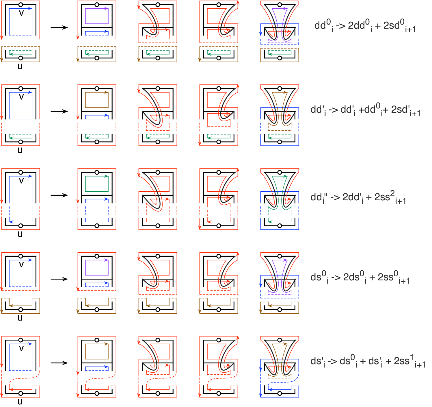
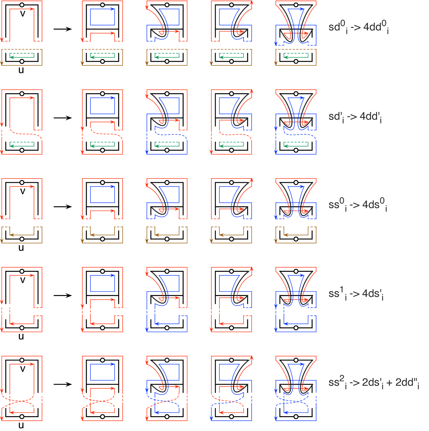
A production is an algebraic representation of the set of possible effects of a graph operation on a graph embedding. For instance, adding a rung to an embedded symmetric ladder $(\ddot{L}_{n},u,v)$ involves inserting a new vertex on each side of the root-vertex $v$ and then joining the two new vertices. Since both the resulting new vertices are trivalent, the number of embeddings of $(\ddot{L}_{n+1},u,v)$ that can result is 4. Thus, the sum of the coefficients in the consequent of the production (the right side) is 4. Figures 3.2 and 3.3 are topological derivations of the following ten productions used to derive the partitioned genus distribution of $(\ddot{L}_{n+1},u,v)$ from the partitioned genus distribution of $(\ddot{L}_{n},u,v)$.

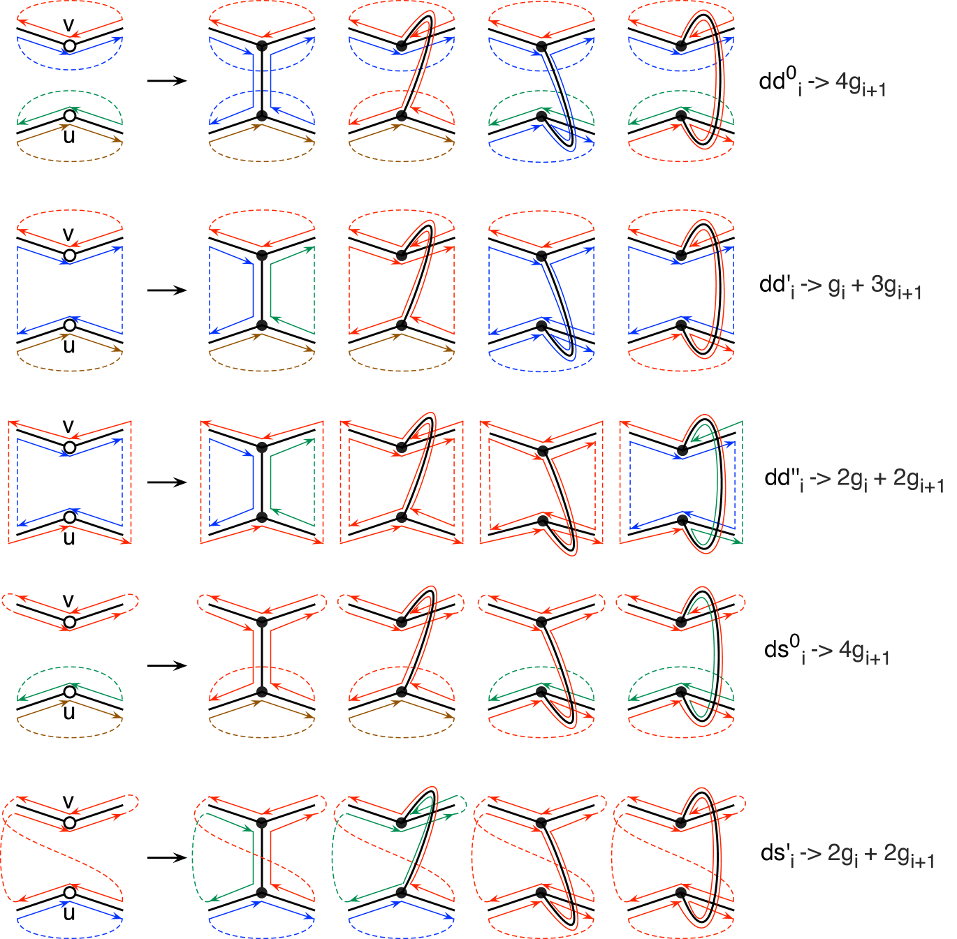
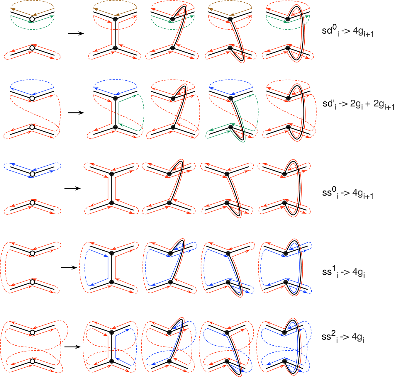
We recall from Section 1 that the self-bar-amalgamation of any doubly vertex-rooted graph $(G,u,v)$, which is denoted $\overline{*}_{uv}(G,u,v)$, is formed by joining the roots $u$ and $v$. The present case of interest is when the two roots are 2-valent and non-adjacent. We observe that if $G$ is a cubic 2-connected graph and if each of the two roots is created by placing a new vertex in the interior of an edge of $G$, then the result of the self-bar amalgamation is again a 2-connected cubic graph.

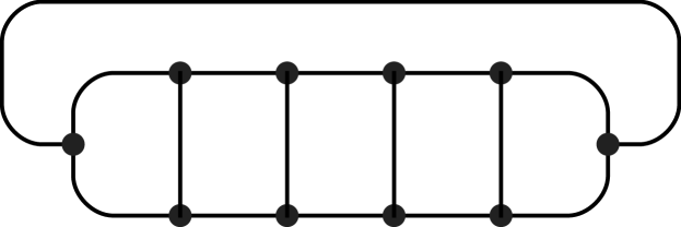
We define a Ringel ladder $RL_{n}$ to be the result of a self-bar-amalgamation on the symmetric ladder $(\ddot{L}_{n},u,v)$. Such ladders were introduced by Gustin [14] and used extensively by Ringel [19] in his solution with Youngs [20] of the Heawood map-coloring problem. The Ringel ladder $RL_{4}$ is illustrated in Figure 5.1. The genus distributions of Ringel ladders were first calculated by Tesar [23]. Our rederivation here is to facilitate our proof of their log-concavity.

To deduce an explicit expression of $\Gamma_{RL_{n}}(x)$, we shall use Chebyshev polynomials. Chebyshev polynomials of the second kind are defined by the recurrence relation

with $U_{0}(x)=1$ and $U_{1}(x)=2x$. It can be equivalently defined by the generating function

• The $p^{\rm th}$ Chebyshev polynomial $U_{p}(x)$ can be expressed by

References

- [1] L.W. Beineke, R.J. Wilson, J.L. Gross, and T.W. Tucker, editors, Topics in Topological Graph Theory, Cambridge Univ. Press, 2009.
- [2] C.P. Bonnington, M. Conder, M. Morton, and P. McKenna, J. Combin. Theory Ser. B 85 (2002), 1–20.
- [3] Y. Chen, J.L. Gross, and X. Hu, Enumeration of digraph embeddings, Euro. J. Combin. 36 (2014), 660–678.
- [4] M. Furst, J.L. Gross and R. Statman, Genus distributions for two class of graphs, J. Combin. Theory Ser. B 46 (1989), 523–534.
- [5] J. L. Gross, Genus distribution of graph amalgamations: Self-pasting at root-vertices, Australasian J. Combin. 49 (2011), 19–38.
- [6] J.L. Gross, Genus distributions of cubic outerplanar graphs, J. of Graph Algorithms and Applications 15 (2011), 295–316.
- [7] J.L.Gross, Embeddings of cubic Halin graphs: a surface-by-surface inventory, Ars Math. Contemporanea 6 (2013), 37–56. Online June 2012.
- [8] J.L. Gross, Embeddings of graphs of fixed treewidth and bounded degree, Ars Math. Contemporanea 7 (2014), 379–403. Online Dec 2013. Presented at AMS Annual Meeting at Boston, January 2012.
- [9] J.L. Gross and M.L. Furst, Hierarchy for imbedding-distribution invariants of a graph, J. Graph Theory 11 (1987), 205–220.
- [10] J.L. Gross, I.F. Khan, and M.I. Poshni, Genus distribution of graph amalgamations: Pasting at root-vertices, Ars Combin. 94 (2010), 33–53.
- [11] J.L. Gross, T. Mansour, T.W. Tucker, and D.G.L. Wang, Log-concavity of combinations of sequences and applications to genus distributions, draft manuscript, 2013.
- [12] J.L. Gross, D.P. Robbins, and T.W. Tucker, Genus distributions for bouquets of circles, J. Combin. Theory Ser. B 47 (1989), 292–306.
- [13] J.L. Gross and T.W. Tucker, Topological Graph Theory, Dover, 2001 (original ed. Wiley, 1987).
- [14] W. Gustin, Orientable embedding of Cayley graphs, Bull. Amer. Math. Soc. 69 (1963), 272–275.
- [15] M. Kotrbcik and M. Skoviera, Matchings, cycle bases, and the maximum genus of a graph, Electronic J. Combin. 19(3) (2012), P3.
- [16] L.L. Liu and Y. Wang, A unified approach to polynomial sequences with only real zeros, Adv. in Appl. Math. 38 (2007), 542–560.
- [17] M.I. Poshni, I.F. Khan, and J.L. Gross, Genus distribution of graphs under edge-amalgamations, Ars Math. Contemp. 3 (2010), 69–86.
- [18] M.I. Poshni, I.F. Khan, and J.L. Gross, Genus distribution of 4-regular outerplanar graphs, Electronic J. Combin. 18 (2011), #P212.
- [19] G. Ringel Map Color Theorem, Springer-Verlag, 1974.
- [20] G. Ringel and J.W.T. Youngs, Solution of the Heawood map-coloring problem, Proc. Nat. Acad. Sci. USA 60 (1968), 438–445.
- [21] S. Stahl, Permutation-partition pairs. III. Embedding distributions of linear families of graphs, J. Combin. Theory, Ser. B 52 (1991), 191–218.
- [22] S. Stahl, On the zeros of some genus polynomials, Canad. J. Math. 49 (1997), 617–640.
- [23] E.H. Tesar, Genus distribution of Ringel ladders, Discrete Math. 216 (2000), 235–252.
- [24] D.G. Wagner, Zeros of genus polynomials of graphs in some linear families, Univ. Waterloo Research Repot CORR 97-15 (1997), 9pp.