Long-living excited states of a 2D diamagnetic exciton

Diamagnetic exciton, a bound state of electron and hole in a magnetic field, was studied theoretically and experimentallySeisyan for many years. Originally, the attention was focused on the bulk semiconductors.Gorkov Later, the interest has shifted to the two-dimensional systems.Lozovik ; Kallin ; Macdonald1986 ; Butov ; Zimmermann It was established that, for interband excitonsLozovik as well as for inter-Landau-level excitons,Kallin that the exciton dispersion law has a local minimum at momenta of the order of the inverse magnetic length.

Recently, Zeeman ; CrookerNano ; Veligzhanin ; Crooker ; Luminescence ; Luminescence1 ; Potemski1 ; Potemski2 ; report the exciton spectroscopy in a perpendicular magnetic field was applied to the novel van der Waals monolayers. These materials host a series of exciton Rydberg states corresponding to the principal quantum number $n=1,2,...$. This property is a consequence of strong Coulomb interaction resulting from the reduced dielectric screening. Experimental spectra in Refs. Zeeman, ; CrookerNano, ; Veligzhanin, ; Crooker, ; Luminescence, ; Luminescence1, ; Potemski1, ; Potemski2, ; report, were interpreted as diamagnetic shifts of the $S$-states of the exciton. The growth of $\Big{[}E_{n}(B)-E_{n}(0)\Big{]}$ with magnetic field, ${\bf B}$, gets faster with increasing $n$. Note, that the $P$-states of the exciton do not show up in the absorption experiments since the matrix element between the vacuum and the $P$-states is zero. However, $P$-states can manifest themselves in luminescence.

In the present paper we consider excited states of a diamagnetic exciton in a weak magnetic field. Our main finding is that a non-quantizing magnetic field still affects strongly the exciton dispersion. The underlying reason is that, due to accidental degeneracy of the excited states, the motion of the center of mass in a finite field couples different states of the internal motion. It is this coupling, together with lifting of the accidental degeneracy due to deviation from Coulomb attraction at short distances,Rytova ; Keldysh that modifies the dispersion law even in a weak magnetic field. We demonstrate that such a modification can give rise to the loop of extrema in the dispersion law. In turn, this loop of extrema leads to anomalous broadening of the exciton absorption line. Another consequence is that, with a minimum in the dispersion law, an exciton is trapped by arbitrarily weak impurity. Since recombination of a trapped exciton with rapidly precessing center of mass requires a big momentum transfer, this state is long-lived.

We start with a standard Hamiltonian of diamagnetic excitonGorkov ; Lozovik ; Butov ; Zimmermann

		$\displaystyle\hat{H}=\frac{1}{2m_{e}}\Big{[}-i\hbar\nabla_{e}+\frac{e}{c}{\bf A}({\bm{r}}_{e})\Big{]}^{2}$
		$\displaystyle+\frac{1}{2m_{h}}\Big{[}-i\hbar\nabla_{h}-\frac{e}{c}{\bf A}({\bm{r}}_{h})\Big{]}^{2}-\frac{e^{2}}{\kappa\big{|}{\bf r_{e}}-{\bf r_{h}}\big{|}}.$		(1)

Here $m_{e}$ and $m_{h}$ are the masses of electron and hole, $\kappa$ is the dielectric constant. Vector potential ${\bm{A}}({\bm{r}})$ is defined as ${\bm{A}}({\bm{r}})=\frac{1}{2}{\bm{B}}\times{\bm{r}}$.

Upon introducing the center of mass and the relative coordinates

$${\bf R}=\frac{m_{e}{\bf r_{e}}+m_{h}{\bf r_{h}}}{m_{e}+m_{h}},~{}~{}{\bf r}={\bf r}_{e}-{\bf r}_{h},$$

(2)

the Hamiltonian Eq. (II) acquires the form

$$\hat{H}=\hat{H}_{cm}({\bm{R}})+\hat{H}_{rel}({\bm{r}})+\hat{H}_{c}({\bm{r}},{\bm{R}}),$$

(3)

where $\hat{H}_{cm}({\bm{R}})$ describes the motion of the center of mass, $\hat{H}_{rel}({\bm{r}})$ describes the relative motion, and $\hat{H}_{c}({\bm{r}},{\bm{R}})$ describes their coupling. Analytical expressions for the three Hamiltonians are the following

	$\displaystyle\hat{H}_{cm}=-\frac{\hbar^{2}}{2M}\Delta_{\bf R},$		(4)
	$\displaystyle\hat{H}_{rel}=-\frac{\hbar^{2}}{2\mu}\Delta_{\bf r}-\frac{e^{2}}{\kappa r}+\frac{\left(eBr\right)^{2}}{8\mu c^{2}}$
	$\displaystyle+i\hbar\Bigl{(}\frac{eB}{2c}\Bigr{)}\Bigl{(}\frac{1}{m_{e}}-\frac{1}{m_{h}}\Bigr{)}\left(y\partial_{x}-x\partial_{y}\right),$		(5)
	$\displaystyle\hat{H}_{c}=i\hbar\frac{eB}{Mc}\left(y\partial_{X}-x\partial_{Y}\right),$		(6)

where $M=m_{e}+m_{h}$ is the net mass and $\mu=m_{e}m_{h}/(m_{e}+m_{h})$ is the reduced mass of the exciton.

In the absence of magnetic field, the states $n=2$ of the exciton are triply degenerate. At finite field, the degeneracy is lifted by the third and the fourth terms in $\hat{H}_{rel}$. Due to the third term, diamagnetic shifts are different for the $S$ and $P$-states. Fourth term results in the repulsion of the two $P$-states. In addition, the $S$ and $P$-states are coupled to each other via the center-of-mass motion. This coupling is promulgated by the Hamiltonian $\hat{H}_{c}$. Our main point is that the interplay of the three effects leads to a nontrivial modification of the dispersion law of the exciton. In contrast to Refs. Lozovik, ; Kallin, , this nontrivial modification takes place at low fields, so that all three effects can be taken into account perturbatively.

Explicit form of the $n=2$ wavefunctions is the following

		$\displaystyle\psi_{0}({\bm{r}})=C_{0}\Big{(}1-\frac{r}{l}\Big{)}\exp\left[-\frac{r}{2l}\right],$		(7)
		$\displaystyle\psi_{x}({\bm{r}})=C_{x}\left(\frac{x}{l}\right)\exp\left[-\frac{r}{2l}\right],~{}\psi_{y}({\bm{r}})=C_{y}\left(\frac{y}{l}\right)\exp\left[-\frac{r}{2l}\right],$		(8)

where $l$ is expressed via the Bohr radius $a_{B}=\frac{\hbar^{2}\kappa}{\mu e^{2}}$ as $l=\frac{3}{4}a_{B}$. The wavefunctions Eq. (7) correspond to the binding energy $\frac{4}{9}E_{B}$, where $E_{B}=\frac{\mu e^{4}}{2\hbar^{2}\kappa^{2}}$ is the Bohr energy. Normalization constants are the same for all three functions

$$C_{0}=C_{x}=C_{y}=\frac{1}{\left(6\pi\right)^{1/2}l}.$$

(9)

With the help of the wavefunctions Eq. (7) we calculate the diamagnetic shifts

$\displaystyle E_{S}=\frac{e^{2}B^{2}}{8\mu c^{2}}\Big{<}r^{2}\Big{>}_{S},~{}~{}E_{P}=\frac{e^{2}B^{2}}{8\mu c^{2}}\Big{<}r^{2}\Big{>}_{P}.$

(10)

Elementary integration yields

$$\Big{<}r^{2}\Big{>}_{S}=26l^{2},~{}~{}~{}\Big{<}r^{2}\Big{>}_{P}=20l^{2}.$$

(11)

Thus, the shifts of $2S$ and $2P$ states are related as $E_{S}=1.3E_{P}$, with $2S$ state being higher.

Next we evaluate the coupling coefficient between the states $\psi_{0}$ and $\psi_{x},\psi_{y}$. As follows from the form of the Hamiltonian $\hat{H}_{c}$, this matrix element contains

$$x_{SP}=\int d{\bf r}\psi_{0}({\bf r})x\psi_{x}({\bf r}).$$

(12)

Using the wavefunctions Eq. (7), we find

$$x_{SP}=C_{0}^{2}\int\limits_{0}^{\infty}drr\int_{0}^{2\pi}d\phi~{}\cos^{2}\phi~{}\frac{r^{2}}{l}\left(1-\frac{r}{l}\right)\exp\left[-\frac{r}{l}\right].$$

(13)

Angular integration yields $\pi$. Performing the radial integration, we find

$$x_{SP}=\pi C_{0}^{2}\int\limits_{0}^{\infty}dr~{}\frac{r^{3}}{l}\left(1-\frac{r}{l}\right)\exp\left[-\frac{r}{l}\right]=-3l.$$

(14)

Since the Hamiltonian $\hat{H}_{c}$ contains $\partial_{X}$ and $\partial_{Y}$, the coupling between the $S$ and $P$-states depends on the motion of the center of mass. If the center of mass moves with momentum, $Q$, the general form of the exciton wavefunction can be presented as a linear combination

$\displaystyle\Psi({\bf r},{\bf R})=\exp[i{\bf QR}]\Big{[}A_{0}\psi_{0}({\bm{r}})+A_{x}\psi_{x}({\bm{r}})+A_{y}\psi_{y}({\bm{r}})\Big{]}.$

(15)

Substituting the form Eq. (15) into the Schrödinger equation, ${\hat{H}}\Psi=E\Psi$, yields the system of equations for the coefficients $A_{0},A_{x}$, and $A_{y}$

		$\displaystyle\Bigg{(}\frac{\hbar^{2}Q^{2}}{2M}+E_{S}-E\Bigg{)}A_{0}-\hbar\Omega_{+}x_{SP}(Q_{y}A_{x}-Q_{x}A_{y})=0,$		(16)
		$\displaystyle\Bigg{(}\frac{\hbar^{2}Q^{2}}{2M}+E_{P}-E\Bigg{)}A_{x}-i\hbar\Omega_{-}A_{y}-\hbar\Omega_{+}Q_{y}x_{SP}A_{0}=0,$		(17)
		$\displaystyle\Bigg{(}\frac{\hbar^{2}Q^{2}}{2M}+E_{P}-E\Bigg{)}A_{y}+i\hbar\Omega_{-}A_{x}-\hbar\Omega_{+}Q_{x}x_{SP}A_{0}=0.$		(18)

Here we have introduced two magnetic-field-induced energy scales

$$\hbar\Omega_{-}=\hbar\frac{eB}{2c}\Big{(}\frac{1}{m_{e}}-\frac{1}{m_{h}}\Big{)},~{}\hbar\Omega_{+}=\hbar\frac{eB}{Mc}.$$

(19)

Expressing $A_{x}$, $A_{y}$ from Eqs. (17), (18) and substituting them into Eq. (16), we arrive at the closed equation for the dispersion $E(Q)$

		$\displaystyle\Bigg{(}\frac{\hbar^{2}Q^{2}}{2M}+E_{S}-E\Bigg{)}\Bigg{[}\Bigg{(}\frac{\hbar^{2}Q^{2}}{2M}+E_{P}-E\Bigg{)}^{2}-(\hbar\Omega_{-})^{2}\Bigg{]}$
		$\displaystyle=\Big{(}\hbar\Omega_{+}x_{SP}\Big{)}^{2}Q^{2}\Bigg{(}\frac{\hbar^{2}Q^{2}}{2M}+E_{P}-E\Bigg{)}.$		(20)

Three solutions of Eq. (II) determine three branches of the exciton dispersion. We analyze this dispersion in the next Section.

At short distances between electron and hole their attraction deviates from purely Coulomb as a result of potential created by polarization charges created in the 2D plane, see e.g. Refs. Rytova, ; Keldysh, ; Cudazzo, ; Lewenkopf, ; Dery, . The modified interaction can be parametrized by a single parameter, $r_{0}$, proportional to polarizability, and has a form

$\displaystyle V_{\scriptscriptstyle eff}(\boldsymbol{r})=\frac{\pi e^{2}}{2r_{0}}\Bigg{[}H_{0}\Big{(}\frac{{r}}{r_{0}}\Big{)}-Y_{0}\Big{(}\frac{r}{r_{0}}\Big{)}\Bigg{]},$

(28)

where $H_{0}$ and $Y_{0}$ are the Struve and second-kind Bessel functions, respectively. With modified interaction, the accidental degeneracy of the $n=2$ exciton level is lifted even in the absence of magnetic field. Since the shifts of the $S$ and $P$-levels are relatively small, the deviation of $V_{\scriptscriptstyle eff}(\boldsymbol{r})$ from the Coulomb attraction can be taken into account perturbatively. Corrections to the energy of $S$ and $P$-states read

		$\displaystyle\delta_{S}=\int d{\bf r}\Bigl{(}V_{\scriptscriptstyle eff}(r)-\frac{e^{2}}{\kappa r}\Bigr{)}\psi_{0}({\bm{r}})^{2},$
		$\displaystyle\delta_{P}=\int d{\bf r}\Bigl{(}V_{\scriptscriptstyle eff}(r)-\frac{e^{2}}{\kappa r}\Bigr{)}\psi_{x}({\bm{r}})^{2}.$		(29)

It is convenient to evaluate $\delta_{S}$ and $\delta_{P}$ in the momentum space. For this purpose, we present the Fourier transform of $V_{\scriptscriptstyle eff}(\boldsymbol{r})$ in the form

$$\Phi(q)=-\frac{2\pi e^{2}}{\kappa q}\Big{(}1-\frac{qr_{0}}{1+qr_{0}}\Big{)}$$

(30)

and treat the second term as a perturbation. Then the expressions for $\delta_{S}$, $\delta_{P}$ take the form

$\displaystyle\delta_{S}=\frac{2\pi e^{2}r_{0}}{\kappa}\int\frac{d{\bf q}~{}q}{1+qr_{0}}U_{0}(q),~{}\delta_{P}=\frac{2\pi e^{2}r_{0}}{\kappa}\int\frac{d{\bf q}~{}q}{1+qr_{0}}U_{x}({\bf q}),$

(31)

where $U_{0}(q)$ and $U_{x}({\bf q})$ stand for the Fourier transforms

		$\displaystyle U_{0}(q)=\int d{\bf r}\psi_{0}({\bm{r}})^{2}\exp\left(i{\bf qr}\right),$
		$\displaystyle U_{x}({\bf q})=\int d{\bf r}\psi_{x}({\bm{r}})^{2}\exp\left(i{\bf qr}\right).$		(32)

In the first transform, angular integration of $\exp\left(i{\bf qr}\right)$ yields the zero-order Bessel function, $J_{0}(qr)$. Then the radial integration is performed with the help of the identity

$\displaystyle\int\limits_{0}^{\infty}d{t}J_{0}(t)\exp\left({-\gamma t}\right)=\frac{1}{(\gamma^{2}+1)^{1/2}}.$

(33)

The result reads

$$U_{0}(q)=\frac{1-3q^{2}l^{2}+q^{4}l^{4}}{\left(1+q^{2}l^{2}\right)^{7/2}}.$$

(34)

Substituting this result into Eq. (IV), we rewrite $\delta_{S}$ in the dimensionless form

$\displaystyle\delta_{S}=\frac{e^{2}}{\kappa l}F_{S}\left(\frac{r_{0}}{l}\right),~{}F_{S}=\frac{r_{0}}{l}\int\limits_{0}^{\infty}\frac{dQQ}{1+\frac{r_{0}}{l}Q}\frac{1-3Q^{2}+Q^{4}}{\left(1+Q^{2}\right)^{7/2}}.$

(35)

We see that the integral is a function of the dimensionless ratio $r_{0}/l$.

Angular integration in $U_{x}({\bf q})$ is less trivial. This is because both the exponent $\exp\left(i{\bf qr}\right)$ and the pre-exponential factor contain the angle $\phi_{\bf r}$. One has

	$\displaystyle U_{x}({\bf q})=C^{2}_{0}\!\!\int\limits_{0}^{2\pi}\int\limits_{0}^{\infty}d{\phi_{\bf r}}drr\Big{(}\frac{r\cos\phi_{\boldsymbol{r}}}{l}\Big{)}^{2}\!\exp\Big{(}-\frac{r}{l}\Big{)}$
	$\displaystyle\times\exp\Big{(}iqr\cos(\phi_{{\bf q}}-\phi_{\boldsymbol{r}})\Big{)}.$		(36)

The result of integration contains a constant part and two other parts proportional to $\cos(2\phi_{\bf q})$ and $\sin(2\phi_{\bf q})$. Only a constant part contributes to $\delta_{P}$. To calculate this constant part it is sufficient to replace $\cos\phi_{\boldsymbol{r}}^{2}$ by $1/2$. Subsequent steps are similar to those in calculation of $\delta_{S}$ and leads to the result

$$\delta_{P}=\frac{e^{2}}{\kappa l}F_{P}\left(\frac{r_{0}}{l}\right),~{}F_{P}=\frac{r_{0}}{l}\int\limits_{0}^{\infty}\frac{dQQ}{1+\frac{r_{0}}{l}Q}\frac{1-\frac{3}{2}Q^{2}}{\left(1+Q^{2}\right)^{7/2}}.$$

(37)

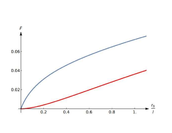
At small $r_{0}\ll l$ the integral is proportional to $r_{0}$. This is a consequence of the fact that the wavefunction of the $P$-state turns to zero at the origin. The functions $F_{S}\left(\frac{r_{0}}{l}\right)$ and $F_{P}\left(\frac{r_{0}}{l}\right)$ are plotted in Fig. 3. Realistic value of $\frac{r_{0}}{l}$ for transition-metal dichalcogenides can be estimated e.g. using the data of Ref. Crooker, . From the spectroscopic measurements the value $r_{0}\approx 3.5$nm was inferred, while the radius of the ground-state wavefunction $a_{B}\approx 1.5$nm. Thus, for the first excited state, the ratio $\frac{r_{0}}{l}$ is $\sim 1$.

Corrections $\delta_{S}$, $\delta_{P}$ are independent of magnetic field, while $E_{S}$ and $E_{P}$ are proportional to $B^{2}$. Thus, the difference

$$E_{SP}=\Big{(}E_{S}+\delta_{S}\Big{)}-\Big{(}E_{P}+\delta_{P}\Big{)}$$

(38)

is a linear function of magnetic field. Two other parameters, $\hbar\Omega_{-}$ and $\varepsilon_{0}$, which enter into the equation Eq. (II), are proportional to $B$ and to $B^{2}$, respectively. Overall, the evolution of the exciton branches with magnetic field is quite nontrivial. To examine this evolution, we turn to the analytical solutions of the cubic equation. The shortest way to arrive to these solutions is performing the following substitution in Eq. (II)

$$E=\frac{\hbar^{2}Q^{2}}{2M}+\frac{E_{SP}}{3}-\Bigg{[}\frac{E_{SP}^{2}}{3}+\left(\hbar\Omega_{-}\right)^{2}+\varepsilon_{0}\frac{\hbar^{2}Q^{2}}{2M}\Bigg{]}^{1/2}\eta,$$

(39)

Then the cubic equation for $\eta$ assumes the form

$$\eta^{3}-\eta+f=0.$$

(40)

Here the dimensionless parameter $f$ is the following combination of $E_{SP}$, $\hbar\Omega_{-}$, and $\varepsilon_{0}$

$$f(Q)=\frac{E_{SP}\Big{[}\frac{2}{9}E_{SP}^{2}-2\left(\hbar\Omega_{-}\right)^{2}+\varepsilon_{0}\frac{\hbar^{2}Q^{2}}{2M}\Big{]}}{3\Big{[}\frac{1}{3}E_{SP}^{2}+\left(\hbar\Omega_{-}\right)^{2}+\varepsilon_{0}\frac{\hbar^{2}Q^{2}}{2M}\Big{]}^{3/2}}.$$

(41)

Three solutions of Eq. (40) can be easily expressed via the phase $\varphi$ defined as

$$\varphi(Q)=\arctan\left\{\frac{1}{f(Q)}\left(\frac{4}{27}-f(Q)^{2}\right)^{1/2}\right\}.$$

(42)

Analytical form of these solutions is the following

$\displaystyle\eta_{0}=-\frac{2}{\sqrt{3}}\cos\Big{(}\frac{\varphi}{3}\Big{)},~{}\eta_{\pm}=-\frac{2}{\sqrt{3}}\cos\Big{(}\frac{\varphi}{3}\pm\frac{2\pi}{3}\Big{)}.$

(43)

We see that the character of solutions changes as $f$ passes through the value $\frac{2}{3^{3/2}}$, when the phase passes through zero. In particular, for $Q=0$ the value $f=\frac{2}{3^{3/2}}$ is achieved under the condition $E_{SP}=\hbar\Omega_{-}$. In fact, this condition corresponds to the linear crossing of the two branches. Introducing the deviation

$$\hbar\Omega_{-}-E_{SP}=\Delta$$

(44)

and expanding Eq. (II) at small $Q$ and $\Delta$, we find behavior of two close branches near the condition $E_{SP}=\hbar\Omega_{-}$

$$E=\frac{\hbar^{2}Q^{2}}{2M}+\frac{\Delta}{2}\pm\Bigg{[}\left(\frac{\Delta}{2}\right)^{2}+\frac{\varepsilon_{0}}{2}\left(\frac{\hbar^{2}Q^{2}}{2M}\right)\Bigg{]}^{1/2}.$$

(45)

We see that a gap of a width, $\Delta$, opens in the spectrum at finite $\Delta$.

Finally, by expanding Eq. (II), we find the behavior of all three branches near $Q=0$

		$\displaystyle E=E_{SP}+\frac{\hbar^{2}Q^{2}}{2M}\Bigg{[}1+\frac{\varepsilon_{0}E_{SP}}{E_{SP}^{2}-\left(\hbar\Omega_{-}\right)^{2}}\Bigg{]},$		(46)
		$\displaystyle E=-\hbar\Omega_{-}+\frac{\hbar^{2}Q^{2}}{2M}\Bigg{[}1-\frac{\varepsilon_{0}}{2\left(E_{SP}+\hbar\Omega_{-}\right)}\Bigg{]},$		(47)
		$\displaystyle E=\hbar\Omega_{-}+\frac{\hbar^{2}Q^{2}}{2M}\Bigg{[}1-\frac{\varepsilon_{0}}{2\left(E_{SP}-\hbar\Omega_{-}\right)}\Bigg{]}.$		(48)

We conclude that negative effective mass at $Q=0$ emerges at $\left(E_{SP}\pm\hbar\Omega_{-}\right)<\frac{1}{2}\varepsilon_{0}$. Approaching of denominators in Eqs. (47), (48) to zero signals the proximity to the exciton resonance.

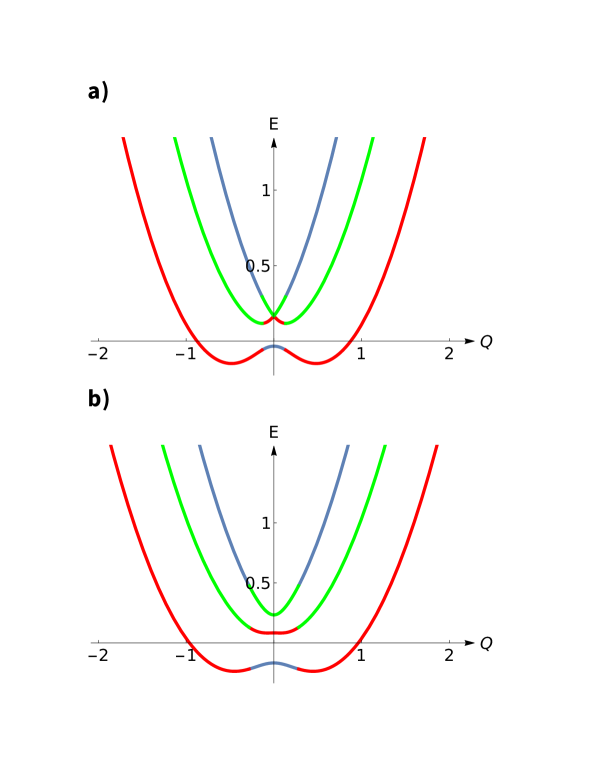
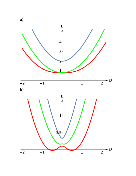
Our most nontrivial finding is the exciton resonance originating from the accidental degeneracy of the hydrogen-like excited levels. The resonant condition reads $E_{SP}=\pm\hbar\Omega_{-}$. It corresponds to the magnetic field at which the mismatch of $S$ and $P$ exciton levels due to diamagnetic shift as well as due to field-independent Keldysh potential, is equal to the field-induced splitting of the degenerate $P$-states. All three branches of the bare exciton spectrum ($S$-branch and two $P$-branches) are involved into the formation of the resonance. Under the resonant condition, two branches of the modified spectrum cross linearly, as illustrated in Fig. 1a. Away from the resonance, see Figs. 1b and 2b, the lowest branch of the spectrum evolves into a “mexican hat” as predicted by Eqs. (27), (23) for the limiting cases $E_{SP}\ll\hbar\Omega_{-}$ and $E_{SP}\gg\hbar\Omega_{-}$, respectively. The main condition for the strong mixing of the $S$ and $P$-branches is $\varepsilon_{0}>\left(E_{SP}+\hbar\Omega_{-}\right)$. We have demonstrated that, neglecting the Keldysh shift, and for $m_{e}=m_{h}$ this condition is satisfied. Physically, it requires that the matrix element, $x_{SP}$, defined by Eq. (12) is big enough. When this condition is violated, the effective masses for all three branches of the modified spectrum are positive, as illustrated in Fig. 1a.

With regard to physical consequences of the spectrum modification into a mexican hat, it is knownEfros ; Galstyan ; Mkhitaryan ; Voloshin that the density of states near the minimum behaves as $\big{(}E-E_{min}\big{)}^{-1/2}$, i.e. it has a one-dimensional character. As a result, even a weak attractive impurity can trap an exciton. The wave function of the trapped exciton is centered around $Q_{min}$ in the momentum space. With $Q_{min}$ exceeding the momentum of a photon required for radiative recombination, these trapped states are long-lived.

Throughout the paper we considered the simplest model of diamagnetic exciton without account for the valley effects which lead to the polarization dependence of the optical absorption as well as the spin-orbit effects leading to the dark-bright exciton mixing.Durnev We have also assumed that the coupling of the $S$ and $P$-exciton states is exclusively due to magnetic field and not by the peculiarities of the bandstructure of dichalcogenide monolayers.Glazov

While the optical absorption probes only the $S$-states of the exciton, finite-momentum states can be probed in the microcavity setting.microcavity Another consequence of the field-induced modification of the exciton spectrum is anomalous broadening of $n=2$ absorption line. The underlying mechanismsemimagnetic ; WithDisorder is the elastic scattering of $Q=0$ state into the states with finite center-of-mass momentum, $Q$. This scattering is enabled by the mexican-hat shape of the spectrum.

The work was supported by the Department of Energy, Office of Basic Energy Sciences, Grant No. DE- FG02- 06ER46313.

References

- (1) see e.g. the review R. P. Seisyan and B. P. Zakharchenya, “Interband magneto-optics of semiconductors as diamagnetic exciton spectroscopy,” in Modern Problems in Condensed Matter Sciences, Elsevier 27, 345 (1991).
- (2) L. P. Gorkov and I. E. Dzyaloshinskii, “Contribution to the theory of the Mott exciton in a strong magnetic field,” Zh. Eksp. Teor. Fiz. 53, 717 (1967) [Sov. Phys. JETP 26, 449 (1968)].
- (3) I. V. Lerner and Yu. E. Lozovik, “Mott exciton in a quasi-two-dimensional semiconductor in a strong magnetic field,” Zh. Eksp. Teor. Fiz. 78, 1167 (1980) [Sov. Phys. JETP 51, 588 1980].
- (4) C. Kallin and B. I. Halperin, “Excitations from a filled Landau level in the two-dimensional electron gas,” Phys. Rev. B 30 5655, (1984).
- (5) A. H. MacDonald and D. S. Ritchie, “Hydrogenic energy levels in two dimensions at arbitrary magnetic fields,” Phys. Rev. B 33 8336 (1986).
- (6) Yu. E. Lozovik, I. V. Ovchinnikov, S. Yu. Volkov, L. V. Butov, and D. S. Chemla, “Quasi-two-dimensional excitons in finite magnetic fields,” Phys. Rev. B, 65, 235304 (2002).
- (7) M. Grochol, F. Grosse, and R. Zimmermann, “Exciton wave function properties probed by diamagnetic shift in disordered quantum wells,” Phys. Rev. B 71, 125339 (2005).
- (8) Y. Li, J. Ludwig, T. Low, A. Chernikov, X. Cui, G. Arefe, Y. D. Kim, A. M. van der Zande, A. Rigosi, H. M. Hill, S. H. Kim, J. Hone, Z. Li, D. Smirnov, and T. F. Heinz, “Valley Splitting and Polarization by the Zeeman Effect in Monolayer MoSe2,” Phys. Rev. Lett. 113, 266804 (2014).
- (9) A. V. Stier, N. P. Wilson, G. Clark, X. Xu, and S. A. Crooker, “Probing the Influence of Dielectric Environment on Excitons in Monolayer WSe2: Insight from High Magnetic Fields,” Nano Lett. 16, 7054 (2016).
- (10) A. V. Stier, N. P. Wilson, K. A. Velizhanin, J. Kono, X. Xu, and S. A. Crooker, “Magnetooptics of Exciton Rydberg States in a Monolayer Semiconductor,” Phys. Rev. Lett. 120, 057405 (2018).
- (11) M. Goryca, J. Li, A. V. Stier, T. Taniguchi, K. Watanabe, E. Courtade, S. Shree, C. Robert, B. Urbaszek, X. Marie, and S. A. Crooker, “Revealing exciton masses and dielectric properties of monolayer semiconductors with high magnetic fields,” Nat. Commun. 10, 4172 (2019).
- (12) E. Liu, J. van Baren, T. Taniguchi, K. Watanabe, Y.-C. Chang, and C. H. Lui, “Magnetophotoluminescence of exciton Rydberg states in monolayer WSe2,” Phys. Rev. B 99, 205420 (2019).
- (13) S.-Y. Chen, Z. Lu, T. Goldstein, J. Tung, A. Chaves, J. Kunstmann, L. S. R. Cavalcante, T. Woznyak, G. Seifert, D. R. Reichman, T. Taniguchi, K. Watanabe, D. Smirnov, and J. Yan, “Luminescent emission of excited Rydberg excitons from monolayer WSe2,” Nano Lett. 19, 2464 (2019).
- (14) M. R. Molas, A. O. Slobodeniuk, K. Nogajewski, M. Bartos, L. Bala, A. Babinski, K. Watanabe, T. Taniguchi, C. Faugeras, and M. Potemski, “Energy spectrum of two-dimensional excitons in a non-uniform dielectric medium,” Phys. Rev. Lett. 123, 136801 (2019).
- (15) P. Kapuscinski, A. Delhomme, D. Vaclavkova, A. Slobodeniuk, M. Grzeszczyk, M. Bartos, K. Watanabe, T. Taniguchi, C. Faugeras, and M. Potemski, “Rydberg series of dark excitons and the conduction band spin-orbit splitting in monolayer WSe2” arXiv:2102.12286.
- (16) J. Jadczak, J. Kutrowska-Girzycka, T. Smolenski, P. Kossacki, Y. S. Huang, and L. Bryja, “Exciton binding energy and hydrogenic Rydberg series in layered ReS2,” Sci. Rep. 9, 1578 (2019).
- (17) N. S. Rytova, “Screened potential of a point charge in a thin film,” Moscow University Physics Bulletin 3, 30 (1967)
- (18) L. V. Keldysh, “Coulomb interaction in thin semiconductor and semimetal films,” JETP Lett. 29, 658 (1979).
- (19) P. Cudazzo, I. V. Tokatly, and A. Rubio, “Dielectric screening in two-dimensional insulators: Implications for excitonic and impurity states in graphane,” Phys. Rev. B 84, 085406 (2011).
- (20) E. Ridolfi, C. H. Lewenkopf, and V. M. Pereira, “Excitonic structure of the optical conductivity in MoS2 monolayers, Phys. Rev. B 97, 205409 (2018).
- (21) D. V. Tuan, M. Yang, and H. Dery, “The Coulomb interaction in monolayer transition-metal dichalcogenides,” Phys. Rev. B 98, 125308 (2018).
- (22) M. E. Raikh and Al. L. Efros, “Broadening of an exciton line in solid solutions with a degenerate valence band,” JETP Lett. 45, 380 (1987).
- (23) A. G. Galstyan and M. E. Raikh, “Disorder-Induced Broadening of the Density of States for 2D Electrons with Strong Spin-Orbit Coupling,” Phys. Rev. B 58, 6736 (1998).
- (24) V. V. Mkhitaryan and M. E. Raikh, “Disorder-induced tail states in a gapped bilayer graphene,” Rev. B 78, 195409 (2008).
- (25) B. Skinner, B. I. Shklovskii, and M. B. Voloshin, “Bound state energy of a Coulomb impurity in gapped bilayer graphene,” Phys. Rev. B 89, 0414059(R) (2014).
- (26) M. V. Durnev and M. M. Glazov, “Excitons and trions in two-dimensional semiconductors based on transition metal dichalcogenides,” Phys. Usp. 61, 825 (2018).
- (27) M. M. Glazov, L. E. Golub, G. Wang, X. Marie, T. Amand, and B. Urbaszek, “ Intrinsic exciton-state mixing and nonlinear optical properties in transition metal dichalcogenide monolayers,” Phys. Rev. B 95, 035311 (2017).
- (28) V. Walther, R. Johne, and T. Pohl, “Giant optical nonlinearities from Rydberg excitons in semiconductor microcavities,” Nature communications, Nat. Commun. 9, 1309 (2018).
- (29) M. E. Raikh and Al. L. Efros, “Exciton line broadening in a semimagnetic semiconductor,” Sov. Phys.-Solid State 30, 1708 (1988).
- (30) M. Dwedari, S. Brem, M. Feierabend, and E. Malic, “Disorder-induced broadening of excitonic resonances in transition metal dichalcogenide,” Phys. Rev. Mater. 3, 074004 (2019).