Long-range correlation and multifractality in Bach’s Inventions pitches
Abstract
We show that it can be considered some of Bach pitches series as a stochastic process with scaling behavior. Using multifractal deterend fluctuation analysis (MF-DFA) method, frequency series of Bach pitches have been analyzed. In this view we find same second moment exponents (after double profiling) in ranges () in his works. Comparing MF-DFA results of original series to those for shuffled and surrogate series we can distinguish multifractality due to long-range correlations and a broad probability density function. Finally we determine the scaling exponents and singularity spectrum. We conclude fat tail has more effect in its multifractality nature than long-range correlations.
pacs:
02.50.Fz, 05.45.TpPythagoras knew it, but Bach demonstrated it: without mathematics there is no music Noralv .
I Introduction
Many people think that, mathematics and music have some vague sort of affinity, but most often supposed relationship between two fields turns out to be in details that are not central to either. The mathematical proportions in musical works are hidden from listener from old days. Thus it is forced to make use of interpretative techniques in order to search for them, which is problematic from a methodological point of view. Some music historians have very little time for numerology. In addition to mathematics being seen as numerical symbolism, music is closely linked to absolute physical entities, such as frequency and relation between intervals (an interval is space between two notes). Already in antiquity this was seen as natural or cosmic premise on which music relied. It is illustrated fact that not just musical notation, but also relationship between music and time has something to do with mathematics and with one of the most significant transformations in music history. Complexity of music can be especially attracting scientific interest. Among great variety of complex and disordered systems most of music parameters such as frequency and pitch (Pitch is the sound frequency of any given note.) lyan ; Heather ; Jafari ; Gonzalez ; Shi , Amplitude or Dynamics (Dynamics are the changes in volume during a musical piece.) Diodati ; Jean , Intervals (Intervals are the distances between notes in the musical scale.), Rhythm (Rhythm is the structure of the placement of notes in musical time.) can be consider as stochastic processes. Also, some authors try to clustering the music Rudi1 ; Rudi2 .
In all technicalities, music can be composed of notes. A note is a sign used in music to represent the relative duration and pitch of sound. In traditional music theory pitch classes are represented by the first seven letters of the Latin alphabet (A, B, C, D, E, F, and G) or (Do - Re - Mi - Fa - Sol - La - Si), in Italian notation. Each note is assigned a specific vertical position on a staff. Since the physical causes of music are vibrations of mechanical systems, their frequencies are often measured in hertz (Hz). These frequencies are mathematically related to each other, and are defined around the central note. The current ”standard pitch” for this note is 440 Hz. Any note is exactly an integer number of half-steps away from central note. Let this distance be denoted n. Then, the desired frequency is given by
| (1) |
In this paper we would like to characterize complex behavior of frequency of note signal of Bach’s Inventions and Sinfonias through computation of signal parameters scaling exponents, which quantifies correlation exponents and multifractality of signal. Inventions and Sinfonias are collection of short pieces which Bach wrote for musical education of Bach young pupils. These are among finest examples of artistic gems ever written for this purpose, and probably because of this, they became very popular among Bach’s pupils and others ever since they were written. Inventions and Sinfonias contain two and three music voices respectively. The number of the data in frequency series is dependent to the piece and will obtain from one voice which contains 1000 notes in average. Because of non-stationary nature of frequency of music series, and due to finiteness of available data sample, we should apply a methods which are insensitive to non-stationarities, like trends. In order to separate trends from correlations we need to eliminate trends in our frequency data. Several methods are used effectively for this purpose: detrended fluctuation analysis (DFA) Peng94 , rescaled range analysis (R/S) hurst65 and wavelet techniques (WT) wtmm .
We use MF-DFA method for analysis and eliminating trend from data set. This method are the modified version of DFA method to detect multifractal properties of time series. DFA method introduced by Peng et al. Peng94 has became a widely used technique for the determination of (mono-) fractal scaling properties and the detection of long-range correlations in noisy, non-stationary time series murad ; physa ; kunhu ; kunhu1 . It has successfully been applied to diverse fields such as DNA sequences Peng94 ; dns , heart rate dynamics herz ; Peng95 ; PRL00 , neuron spiking neuron , human gait gait , wind speed, Govindan , long-time weather records wetter , cloud structure cloud , geology malamudjstatlaninfer1999 , ethnology Alados2000 , economical time series economics , and solid state physics fest . One reason to employ DFA method is to avoid spurious detection of correlations that are artefacts of non-stationarity in time series.
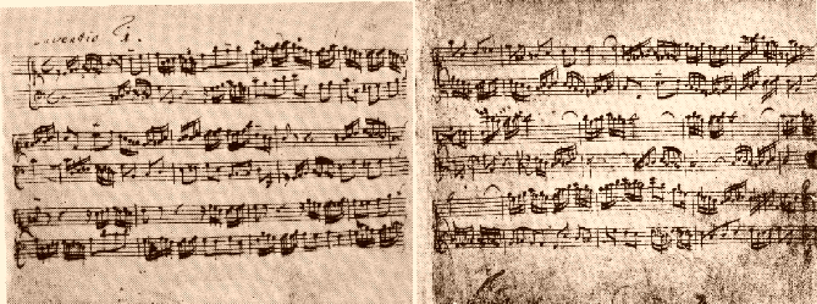
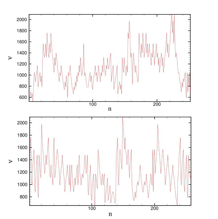
The focus of present paper is on intriguing statistical properties and multifractal nature of frequency series. In Particular, Figures 1 and 2 show the score of Invention no.1 and the frequency fluctuation of Invention no. 1 and Sinfoina no. 1, respectively. In general, two different types of multifractality in frequency series can be distinguished: (i) Multifractality due to a fatness of probability density function (PDF) of time series. In this case multifractality cannot be removed by shuffling the series. (ii) Multifractality due to different long-range correlations in small and large scale fluctuations. In this case data may have a PDF with finite moments, e.g. a Gaussian distribution. Thus corresponding shuffled time series will exhibit mono-fractal scaling, since all long-range correlations are destroyed by shuffling procedure. If both kinds of multifractality are present, shuffled series will show weaker multifractality than original series.
The paper is organized as follows: In section II we describe MF-DFA
methods in detail and show that, scaling exponents determined by
MF-DFA method are identical to those obtained by standard
multifractal formalism based on partition functions. In section III,
we analysis of frequency series of Bach’s Inventions also examine
source of multifractality in frequency data by comparison MF-DFA
results for remaining data set to those obtained by MF-DFA for
shuffled and surrogate series. section IV
closes with a conclusion.
II Multifractal Detrended Fluctuation Analysis
The simplest type of multifractal analysis is based upon standard partition function multifractal formalism, which has been developed for multifractal characterization of normalized, stationary measurements feder88 ; barabasi ; peitgen ; bacry01 . Unfortunately, this standard formalism does not give us correct results for non-stationary time series that are affected by trends or those which cannot be normalized. In the early 1990s an improved multifractal formalism wavelet transform modulus maxima (WTMM) method wtmm , has been developed. This method is based on wavelet analysis and involves tracing the maxima lines in continuous wavelet transform over all scales. Other method like, multifractal detrended fluctuation analysis (MF-DFA), is based on identification of scaling of th-order moment depending on signal length, and it is generalization of standard DFA method in which . In contrast to WTMM method MF-DFA does not require modulus maxima procedure, and hence does not require more effort in programming and computing time than conventional DFA. On the other hand, one should find correct scaling behavior of fluctuations, from experimental data which often affected by non-stationary like trends. This have to be well distinguished from intrinsic fluctuations of system. In addition often in collected data we do not know reasons, or even worse scales, for underlying trends, and also, usually available record data is small. So for reliable detection of correlations, it is essential to distinguish trends for intrinsic fluctuations from collected data. Hurst rescaled-range analysis hurst65 and other non-detrending methods work well when records are long and do not involve trends, otherwise it might give wrong results. DFA is a well established method for determining scaling behavior of noisy data, where data presence of trends and we don’t know their origin and shape Peng94 ; Peng95 ; fano ; allan ; buldy95 .
II.1 Description of MF-DFA method
Modified multifractal DFA (MF-DFA) procedure consists of five steps. The first three steps are essentially identical to conventional DFA procedure (see e.g. Peng94 ; murad ; physa ; kunhu ; kunhu1 ). Suppose that is a series of length , and it is of compact support, i.e. for an insignificant fraction of the values only.
Step 1: Determine the “profile”
| (2) |
Subtraction of the mean from is not compulsory, since it would be eliminated by later detrending in third step.
Step 2: Divide profile into non overlapping segments of equal lengths . Since length of series is often not a multiple of considered time scale , a short part at the end of profile may remain. In order not to disregard this part of series, same procedure should be repeated starting from the opposite end. Thereby, segments are obtained altogether.
Step 3: Calculate local trend for each of segments by a least-square fit of series. Then determine the variance
| (3) |
for each segment and
| (4) |
for . Where, is fitted polynomial in segment . Linear, quadratic, cubic, or higher order polynomials can be used in the fitting procedure (conventionally called DFA1, DFA2, DFA3, , DFA) Peng94 ; PRL00 . Since detrending of time series is done by subtraction of fited polynomial from profile, different order DFA differ in their capability of eliminating trends in series. In (MF-)DFA trend of order in profile (and equivalently, order in original series) are eliminated. Thus a comparison of results for different orders of DFA allows one to estimate type of the polynomial trend in time series physa ; kunhu .
Step 4: Average over all segments to obtain -th order fluctuation function, defined by:
| (5) |
where, in general, variable can take any real value except zero. , standard DFA procedure is retrieved. Generally we are interested to know how generalized dependent fluctuation functions depend on time scale for different values of . Hence, we must repeat steps 2, 3 and 4 for several time scales . It is apparent that will increase with increasing . Of course, depends on DFA order . By construction, is only defined for .
Step 5: Determine scaling behavior of fluctuation functions by analyzing log-log plots of versus for each value of . If series are long-range power law correlated, then , for large values of , increases as a power-law i.e.,
| (6) |
In general, exponent may depend on . For stationary time series such as, fractional Gaussian noise (fGn), in eq. 2, will have a fractional Brownian motion (fBm) signal, so, . The exponent is identical to well known Hurst exponent Peng94 ; murad ; feder88 . Also for non-stationary signal, such as fBm noise, in eq. 2, will be a sum of fBm signal, so corresponding scaling exponent of is identified by Peng94 ; eke02 . For monofractal time series, is independent of , since scaling behavior of variance is identical for all segments , and averaging procedure in eq.(5) will just give this identical scaling behavior for all values of . If we consider positive values of , the segments with large variance (i.e. large deviation from the corresponding fit) will dominate average . Thus, for positive values of , describes scaling behavior of segments with large fluctuations. For negative values of , segments with small variance will dominate average . Hence, for negative values of , describes scaling behavior of segments with small fluctuations.
II.2 Relation to standard multifractal analysis
For a stationary, normalized series multifractal scaling exponent defined in eq.(6) are directly related to scaling exponent defined by standard partition function based on multifractal formalism as shown below. Suppose that series of length is a stationary, normalized sequence, then detrending procedure in step 3 of MF-DFA method is not required, since no trend has to be eliminated. Thus, DFA can be replaced by standard fluctuation analysis (FA), which is identical to DFA except definition of variance, which is simplified for each segment . In step 3 eq.(3) now becomes :
| (7) |
Inserting this simplified definition into eq.(5) and using eq.(6), we obtain
| (8) |
For simplicity we can assume that length of series is an integer multiple of scale , obtaining and therefore
| (9) |
This corresponds to the multifractal formalism used e.g. in barabasi ; bacry01 . In fact, a hierarchy of exponents similar to our has been introduced based on eq.(9) in barabasi . In order to relate this to standard textbook box counting formalism feder88 ; peitgen , we employ definition of profile in eq.(2). It is evident that term in eq.(9) is identical to sum of numbers within each segment of size . This sum is known as box probability in standard multifractal formalism for normalized series ,
| (10) |
The scaling exponent is usually defined via partition function ,
| (11) |
where is a real as in MF-DFA method, discussed above. Using eq.(10) we see that eq.(11) is identical to eq.(9), and one can obtain analytical relation between two sets of multifractal scaling exponents,
| (12) |
Thus, we see that defined in eq.(6) for MF-DFA is directly related to classical multifractal scaling exponents . Note that, is different from generalized multifractal dimension
| (13) |
that are used instead of in some papers. In this case, while is independent of for a monofractal time series, depends on . Another way to characterize a multifractal series is looking to singularity spectrum , which is related to via a Legendre transform feder88 ; peitgen ,
| (14) |
Here, is the singularity strength or Hölder exponent, while denotes dimension of subset of series that is characterized by . Using eq.(12), we can directly relate and to ,
| (15) |
Hölder exponent denotes monofractality, while in multifractal case, different parts of structure are characterized by different values of , leading to existence of spectrum .
III Analysis of music frequency series
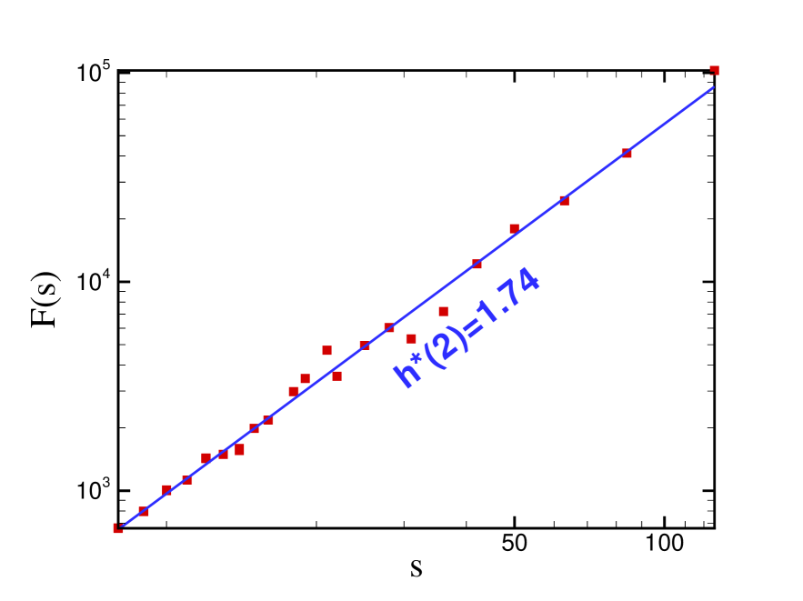
As mentioned in section II, a spurious of correlations may be detected if time series is non-stationarity, so direct calculation of correlation behavior, spectral density exponent, fractal dimensions etc., don’t give us a reliable results. It can be checked out that, frequency series is non-stationary. One can verified non-stationarity property experimentally by measuring stability of average and variance in a moving window for example using scale . According to MF-DFA1 method, generalized Hurst exponents in eq.(6) can be found by analyzing log-log plots of versus for each . Hurst exponent is between . However, the MF-DFA method can only determine positive generalized Hurst exponents, in order to refine the analysis near the fGn/fBm boundary or strongly anti-correlated signals when is close to zero. The simplest way to analyze such data is to integrate the time series before the MF-DFA procedure. Hence, we replace the single summation in Eq. (1), which is describing the profile from the original data, by a double summation by using Classification by the signal summation conversion method (SSC). After using SSC method, fGn switch to fBm and fBm switch to sum-fBm. In this case the relation between the new exponent, , and is eke02 ; Movahed ; bun02 (recently Movahed et al. have proven the relation between derived exponent from double profile of series in DFA method and exponent in Appendix of Movahed ). We find of Invention no. 1 by using SSC method. Note that, the exponents of the new series, after double profiling (SSC), are different from before SSC. Therefore we name these new exponents as , and .
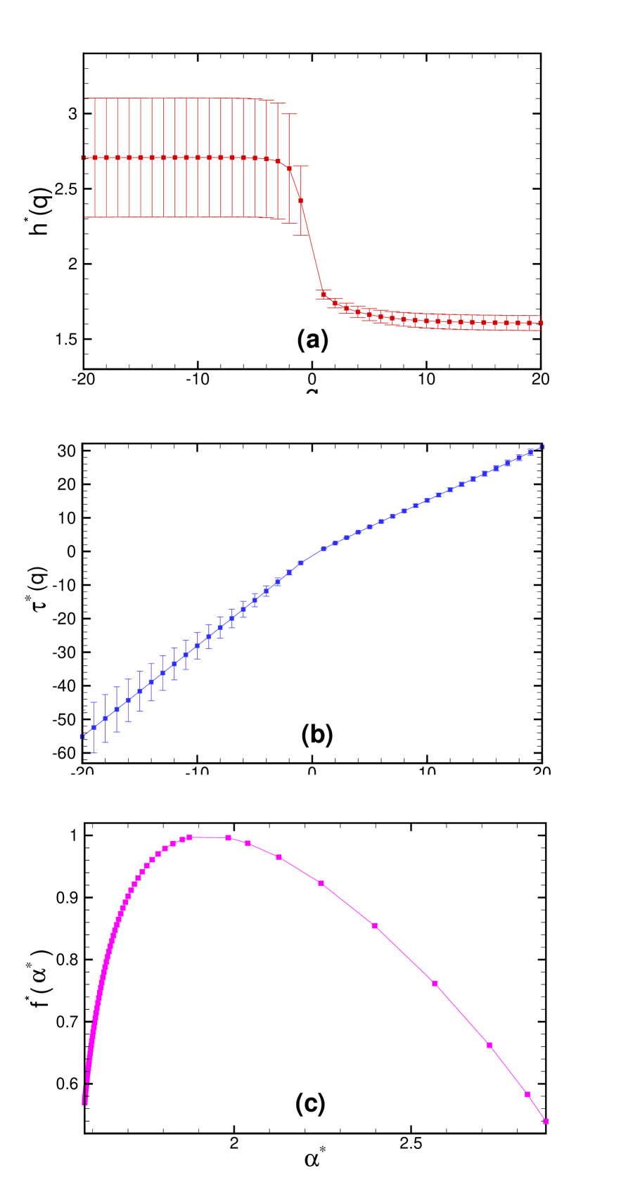
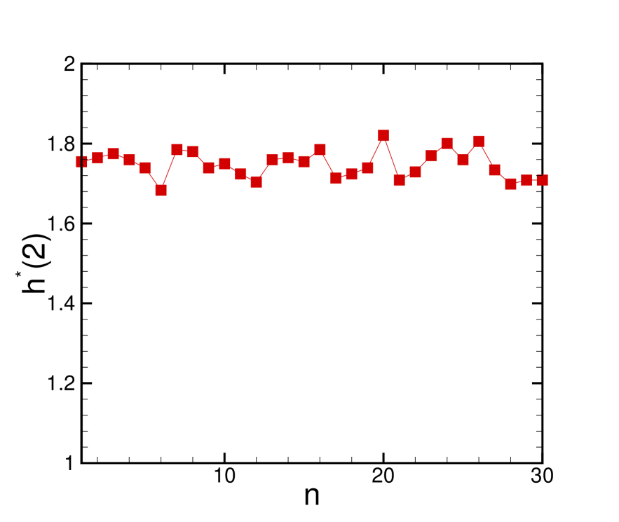
Results using MF-DFA1 method for frequency signal are shown in Figure 4, which shows that frequency series is a multifractal process as indicated by strong dependence of the exponents and bun02 . dependence of the multifractal scaling exponent has linear behaviors for and and slopes of are and , respectively. The values which derived for quantities of MF-DFA1 method for Invention no. 1 are given in Table I. We have calculated exponent for other Inventions and Sinfonias as well, and all of them are in the range (Fig. 5). Figure . 4(c) shows the width of singularity spectrum, , i.e. for the series is approximately, . It value shows the power of multifractality of interevents is very strong paw05 . The values of derived quantities from MF-DFA1 method, are given in Table I. There are some specific lengths in music that have important effects in music’s statistical parameters. a) Rhythm, b) Scale is a set of tones each having a definite pitch (perceived fundamental frequency of a sound) and each having a specific frequency ratio compared to the others, that is, each having specific interval relative to all the other pitches, arranged in a sequence from low to high, or alternatively, from high to low. Composers often transform musical patterns by moving every note in the pattern by a constant number of scale intervals. Since the intervals of a scale can have various sizes, this process introduces subtle melodic and harmonic variation into the music. This variation is what gives scalar music much of its complexity.), c) Bar or measure is a segment of time defined as a given number of beats (the basic time unit of a piece) of a given duration. More over in the Persian music (Eastern music), there are others characteristic lengths such as Gushe which is based on the change of the tonic or stop notes. Existence of these characteristic lengths can effect on music complexity. The music style and more importantly composers can use various the characteristic lengths in the music. We check a few pieces of other genders of music like jazz and Persian traditional music (Eastern music) that obtained in ranges, and , respectively. We find more characteristic lengths in the Persian traditional music which leads to decrease the exponents.
Usually, in MF-DFA method, deviation from a straight line in log-log plot of eq.(6) occurs for small scales . This deviation limits capability of DFA to determine correct correlation behavior for very short scales and in regime of small . The modified MF-DFA is defined as follows physa :
| (16) |
where denotes the usual MF-DFA fluctuation function, defined in eq.(5), averaged over several configurations of shuffled data taken from original time series, and . The values of exponent obtained by modified MF-DFA1 methods for frequency series time series is . The relative deviation of the new exponent which is obtained by modified MF-DFA1 in comparison to MF-DFA1 for original data is less than .
Now, we are interested in to determine source of multifractality. In general, two different types of multifractality in time series can be distinguished: (i) multifractality due to a fatness of probability density function (PDF) of the time series. In this case multifractality cannot be removed by shuffling series. (ii) multifractality due to different correlations in small and large scale fluctuations. In this case data may have a PDF with finite moments, e.g. a Gaussian distribution. Thus corresponding shuffled time series will exhibit mono-fractal scaling, since all long-range correlations are destroyed by shuffling procedure. If both kinds of multifractality are present, shuffled series will show weaker multifractality than original series. The easiest way to clarify the type of multifractality, is by analyzing corresponding shuffled and surrogate time series. Shuffling of time series destroys long-range correlation, therefore if multifractality belongs only to long-range correlation, we should find . The multifractality nature due to fatness of PDF signals is not affected by shuffling procedure. On the other hand, to determine multifractality due to broadness of PDF, phase of discrete fourier transform (DFT) coefficients of frequency series time series are replaced with a set of pseudo independent distributed uniform quantities in surrogate method. The correlations in surrogate series do not change, but probability function changes to Gaussian distribution. If multifractality in time series is due to a broad PDF, obtained by surrogate method will be independent of . If both kinds of multifractality are present in frequency series time series, shuffled and surrogate series will show weaker multifractality than original one.
To check nature of multifractality, we compare fluctuation function , for original series (after cancelation of sinusoidal trend) with result from corresponding shuffled, and surrogate series . Differences between these two fluctuation functions with original one, directly indicate presence of long-range correlations or broadness of probability density function in original series. These differences can be observed in ratio plot of and with respect bun02 . Since anomalous scaling due to a broad probability density affects both of and in same way, only multifractality due to correlations will be observed in . Scaling behavior of these ratios are
| (17) |
| (18) |
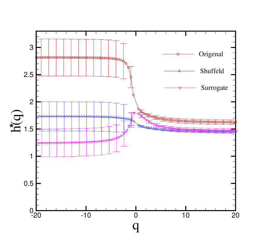
If only fatness of PDF is responsible for multifractality, one should have and . On the other hand, deviations from indicates existence of correlations, and dependence of indicates that multifractality is due to long rage correlation. If only correlation multifractality is present, one finds . If both distribution and correlation multifractality are present, both of and will depend on . The dependence of exponent for original, surrogate and shuffled time series are shown in Figures 6. dependence of and shows that multifractality nature of frequency series time series is due to both broadness of PDF and long-range correlation. Absolute value of is greater than , so multifractality due to correlation is weaker than mulifractality due to fatness.
Deviation of and from can be determined by using test as follows:
| (19) |
symbol can be replaced by and , to determine the confidence level of and to the new exponents, , of original series, respectively. Reduced chi-square ( is number of degree of freedom) for shuffled and surrogate time series are , , respectively. Width of singularity spectrum, , i.e. for original, surrogate and shuffled time series are approximately, , and respectively. These values conclude that multifractality due to fat tail is dominantpaw05 .
Values of the exponents, , and width of singularity spectrum, , for the original, shuffled and surrogate of frequency series obtained with MF-DFA1 method are reported in Table I.
| Original | |||
|---|---|---|---|
| Surrogate | |||
| Shuffled |
IV Conclusion
MF-DFA method allows us to determine multifractal characterization of non-stationary and stationary time series. We have shown that MF-DFA1 result of frequency series of Bach Inventions. Applying MF-DFA1 method is demonstrated that frequency series have long term correlation. We calculated the second moment exponent after the new profile for other Inventions and Sinfonias and they are in the range. dependence of and , shows that frequency series has multifractal behavior. By comparing the second moment exponent of original time series with shuffled and surrogate one’s, we have found that multifractality due to broadness of probability density function has more contribution than correlation in Inventions.
V Acknowledgment
We would like to thank M Sadegh Movahed for reading the manuscript and useful comments. GRJ would like to acknowledge the hospitality extended during his visits at the IPAM, UCLA, where this work was started.
References
- (1) http://www.ntnu.no/
- (2) Julyan H. E. Cartwright, Diego L. Gonz alez, and Oreste Piro, 1999 Phys. Rev. Lett. 82, 5389
- (3) Heather D. Jennings, Plamen Ch. Ivanov, Allan de M. Martins, P.C. da Silva, Viswanathan G M, Physica A 336 (2004) 585 594.
- (4) Jafari G R, Pedram P, Ghafori K, AIP Proceeding (2006).
- (5) Gonzalez D L, Morettini L, Sportolari F, Rosso O, Cartwright J H E and Piro O, arXiv:chao-dyn/9505001, (1995).
- (6) YU SHI, arXiv:adap-org/9509001, (1995).
- (7) Diodati p and Piazz P, Eur. Phys. J. B 17, 143-145.
- (8) Jean Pierre Boon and Olivier Decroly, 1995, Chaos 5(3) 501-508.
- (9) Rudi Cilibrasi, Paul Vitanyi and Ronald de Wolf, Computer Music Journal, 28:4, pp. 49 67, Winter 2004.
- (10) Rudi Cilibrasi and Paul Vitanyi, 2005, IEEE TRANSACTIONS ON INFORMATION THEORY, 51(4), 1523 1545.
- (11) Peng C K, Buldyrev S V, Havlin S, Simons M, Stanley H E, and Goldberger A L, 1994 Phys. Rev. E 49, 1685 ; Ossadnik S M, Buldyrev S B, Goldberger A L, Havlin S, Mantegna R N, Peng C K, Simons M and Stanley H E, 1994 Biophys. J. 67, 64
- (12) Hurst H E, Black R P and Simaika Y M, 1965 Long-term storage. An experimental study (Constable, London)
- (13) Muzy J F, Bacry E and Arneodo A, 1991 Phys. Rev. Lett. 67, 3515
- (14) Taqqu M S, Teverovsky V and Willinger W, 1995 Fractals 3, 785
- (15) Kantelhardt J W, Koscielny-Bunde E, Rego H H A, Havlin S and Bunde A, 2001 Physica A 295, 441
- (16) Hu K, Ivanov P Ch, Chen Z, Carpena P and Stanley H E, 2001 Phys. Rev. E 64, 011114
- (17) Chen Z, Ivanov P Ch, Hu K and Stanley H E, 2002 Phys. Rev. E 65, preprint physics/041107.
- (18) Buldyrev S V, Goldberger A L, Havlin S, Mantegna R N, Matsa M E, Peng C K, Simons M and Stanley H E, 1995 Phys. Rev. E 51, 5084; Buldyrev S V, Dokholyan N V, Goldberger A L, Havlin S, Peng C K, Stanley H E and Viswanathan G M, 1998 Physica A 249, 430
- (19) Ivanov P Ch, Bunde A, Amaral L A N, Havlin S, Fritsch-Yelle J, Baevsky R M, Stanley H E and Goldberger A L, 1999 Europhys. Lett. 48, 594; Ashkenazy Y, Lewkowicz M, Levitan J, Havlin S, Saermark K, Moelgaard H, Thomsen P E B, Moller M, Hintze U and Huikuri H V, 2001 Europhys. Lett. 53, 709; Ashkenazy Y, Ivanov P Ch, Havlin S, Peng C K, Goldberger A L and Stanley H E, 2001 Phys. Rev. Lett. 86, 1900
- (20) Peng C K, Havlin S, Stanley H E and Goldberger A L, 1995 Chaos 5 82
- (21) Bunde A, Havlin S, Kantelhardt J W, Penzel T, Peter J H and Voigt K, 2000 Phys. Rev. Lett. 85, 3736
- (22) Blesic S, Milosevic S, Stratimirovic D and Ljubisavljevic M, 1999 Physica A 268, 275; Bahar S, Kantelhardt J W, Neiman A, Rego H H A, Russell D F, Wilkens L, Bunde A and Moss F, 2001 Europhys. Lett. 56, 454
- (23) Hausdorff J M, Mitchell S L, Firtion R, Peng C K, Cudkowicz M E, Wei J Y and Goldberger A L, 1997 J. Appl. Physiology 82, 262
- (24) Govindon R B and Kantz H, Europhysics letters, 68 (2), pp: 184-190 (2004)
- (25) Koscielny-Bunde E, Bunde A, Havlin S, Roman H E, Goldreich Y and Schellnhuber H J, 1998 Phys. Rev. Lett. 81, 729; Ivanova K and Ausloos M, 1999 Physica A 274, 349; Talkner P and Weber R O, 2000 Phys. Rev. E 62, 150
- (26) Ivanova K, Ausloos M, Clothiaux E E and Ackerman T P, 2000 Europhys. Lett. 52, 40
- (27) Malamud B D and Turcotte D L, 1999 J. Stat. Plan. Infer. 80, 173
- (28) Alados C L and Huffman M A, 2000 Ethnology 106, 105
- (29) Mantegna R N and Stanley H E, 2000 An Introduction to Econophysics (Cambridge University Press, Cambridge); Liu Y, Gopikrishnan P, Cizeau P, Meyer M, Peng C K and Stanley H E, 1999 Phys. Rev. E 60, 1390; Vandewalle N, Ausloos M and Boveroux P, 1999 Physica A 269, 170
- (30) Kantelhardt J W, Berkovits R, Havlin S and Bunde A, 1999 Physica A 266, 461; Vandewalle N, Ausloos M, Houssa M, Mertens P W and Heyns M M, 1999 Appl. Phys. Lett. 74, 1579
- (31) Feder J, 1988 Fractals (Plenum Press, New York)
- (32) Barabási A L and Vicsek T, 1991 Phys. Rev. A 44, 2730
- (33) Peitgen H O, Jürgens H and Saupe D, 1992 Chaos and Fractals (Springer-Verlag, New York), Appendix B
- (34) Bacry E, Delour J and Muzy J F, 2001 Phys. Rev. E 64, 026103
- (35) Fano U, 1947 Phys. Rev. 72 26
- (36) Barmes J A and Allan D W, 1996 Proc. IEEE 54 176
- (37) Buldyrev S V, Goldberger A L, Havlin S, Mantegna R N, Matsa M E, Peng C K, Simons M, Stanley H E, 1995 Phys. Rev. E 51 5084
- (38) Eke A, Herman P, Kocsis L and Kozak L R, 2002 Physiol. Meas. 23, R1-R38
- (39) M Sadegh Movahed, G R Jafari, F Ghasemi , Sohrab Rahvar and M Reza Rahimi Tabar, J. Stat. Mech. (2006) P02003.
- (40) Kantelhardt J W, Zschiegner S A, Kosciliny-Bunde E, Bunde A, Pavlin S and Stanley H E, 2002 Physica A 316, 78-114.
- (41) Oświȩcimka P and et. al, [arXive:cond-mat/0504608]