Long-range interactions and disorder facilitate pattern formation
in spatial complex systems

In his seminal work [1], May studied the time evolution of a well-mixed complex system, where the rate of change of the concentration of each component depends non-linearly on all other components. Such systems are almost certainly stable if interactions are symmetric and the standard deviation of the Jacobian of the linearized system around such states, $\sigma$, is smaller than the inverse square root of the number of components, $L$ (May bound) [1, 2]. This seminal work has been extended to include non-symmetric interactions [3, 4] and dispersion in spatially extended systems, which has a destabilizing effect [5]. Works on models inspired by ecosystems considered stochasticity and showed that the stable regime can exhibit spin-glass behavior and marginally stable states [6, 7]. Global stability is also influenced by the motif structure of interaction networks [8, 9] and kernels [10].

Conditions for stability are particularly relevant in the context of biological systems. For example, in complex ecosystems, the loss of stability can lead to the extinction of species [11]. Further, the integrity of adult tissues relies on stable interactions between cell populations. As complex biological systems often comprise small copy numbers they exhibit strong fluctuations [12]. The strength of these fluctuations typically is concentration-dependent, termed multiplicative noise. Even more than additive noise [13, 14], multiplicative noise can dominate the behavior of stochastic systems [15]. Since interactions in biological systems are often mediated by diffusing agents, they are inherently non-local. For example, in cellular systems diffusing signaling molecules give rise to interactions between cells on a length scale determined by the square root of the product of the diffusion coefficient and the degradation rate [16, 17].

Here, we extend these theoretical works to include these key characteristics of biological systems: non-local interactions and multiplicative noise. Specifically, we study the stability of spatially extended, stochastic complex systems with local and non-local interactions. In order to take into account the role of different noise sources, we start from a general microscopic model and derive the distribution of particle densities stemming from multiplicative noise in a field theoretical framework. Based on this, we derive conditions for stability and characterize the emergence of spatial patterns in the stable regime. We find that non-local interactions destabilize the system by facilitating pattern formation close to the boundary of stability. Multiplicative noise does not alter the conditions for stability on the mean-field level but induces giant density fluctuations in the stable regime, where pattern formation does not occur.

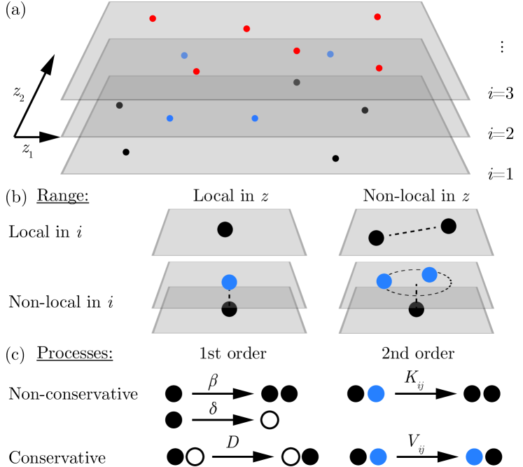
We consider a stochastic many-particle system of $N$ particles, where each particle, indexed by $n$, is characterized by a categorical variable $i\in\{1,\ldots,L\}$ termed component and a position $\vec{z}$ [Fig. 1(a)]. In the context of ecosystems, this describes $N$ individuals belonging to $L$ species which share a habitat. We consider general interactions between particles that can be local or non-local in $\vec{z}$ and in $i$ [Fig. 1(b)] and that may be classified based on whether they conserve global particle numbers or not [Fig. 1(c)]. Within each of these classes, we consider a minimal set of microscopic rules which contribute at most quadratically to the field theory.

Non-conservative interactions comprise a birth-death process with rates $\beta_{i}$ and $\delta_{i}$, respectively. Since interactions are non-local, these rates are functions of the positions of all other particles across components. As a second-order process, we consider Lotka-Volterra type interactions, whereupon a local or non-local interaction between a pair of particles one particle is substituted by a copy of the other. We denote the rate of such interactions between particles of components $i$ and $j$ by $K_{ij}$. In the context of ecosystems, such interactions mimic predator-prey, mutualistic, or competitive interactions between species [18, 19]. Conservative processes globally maintain the number of particles in each component. These comprise particle diffusion with diffusivity $D_{i}$ and, as a minimal process of second order, particles may move along gradients of a two-body potential $V_{ij}(|\vec{z}_{i}-\vec{z}_{j}|)$. We here consider scalar fields, such that processes like rotational diffusion [20] do not contribute to the field theory.

In order to derive a description in terms of a field theory we first define the density of particles at position $\vec{z}$ as $\rho_{i}(\vec{z}\,)=\sum_{n=1}^{N}\delta(\vec{z}_{i}^{n}-\vec{z})$. In the mean-field limit the time evolution of $\mathbf{\rho}(t)$ is then given by a differential equation of the form $\partial_{t}\boldsymbol{\rho}(\vec{z},t)=\boldsymbol{f}[\boldsymbol{\rho}(\vec{z}^{\prime},t)]\,$, where bold symbols represent vectors in $i$. In the following, we will derive expressions for conservative and non-conservative contributions to $\boldsymbol{f}[\boldsymbol{\rho}]$ and effective noise terms from the microscopic processes defining our model.

We begin the analysis by deriving the contributions stemming from non-conservative processes, which are described in the framework of Master equations. Following standard steps [21], we expand the time evolution of the probability distribution in terms of the inverse system size and find that the non-local birth-death process contributes $\mathbf{h}\left[\boldsymbol{\rho},\vec{z}\right]\circ\boldsymbol{\rho}(\vec{z}\,)+\boldsymbol{\eta}$, where $\circ$ denotes the component-wise product and $\boldsymbol{\eta}$ are multiplicative Gaussian white noise with correlations $\langle\eta_{i}(\vec{z},t)\eta_{j}(\vec{z^{\prime}},t^{\prime})\rangle=(\beta_{i}+\delta_{i})\rho_{i}(\vec{z},t)\delta(t-t^{\prime})\delta(\vec{z}-\vec{z}\,^{\prime})\delta_{i,j}$ and $h_{i}=\beta_{i}-\delta_{i}$ [21, 22]. We further make the simplifying assumption that interactions decay exponentially in space with a characteristic length scale denoted by $\zeta_{i}$. With this, we consider a kernel $\mathbf{h}$ of the form,

$$\mathbf{h}[\boldsymbol{\rho},\vec{z}]\approx\mathbf{h}^{0}-\mathbf{h}^{1}\circ\int\text{d}\vec{y}\,e^{-2|\vec{z}-\vec{y}|/\boldsymbol{\zeta}}\circ\boldsymbol{\rho}(\vec{y})\,,$$

(1)

such that the rates $\mathbf{h}^{0}$ and $\mathbf{h}^{1}$ quantify the local and non-local excess rate of birth processes compared to death processes, respectively. With this, we can then express Eq. (1) as a solution of a differential equation for an auxiliary field $\phi(\vec{z},t)$ [23],

$$\phi_{i}-\zeta_{i}^{2}\laplacian\phi_{i}=h^{0}_{i}-h^{1}_{i}\zeta_{i}\rho_{i}\,.$$

(2)

Intuitively, this equation describes the steady state of a field consumed locally by particles and subject to diffusion and degradation. Finally, following Ref. [24] yields that non-conservative two-particle interactions between different components contribute a term $K_{ij}\rho_{i}\rho_{j}$.

In order to derive the contribution of conservative processes we express them in the form of a Langevin equation, which describes stochastic trajectories $\vec{z}_{\,i}^{\,n}(t)$ of individual particles,

$$\partial_{t}\vec{z}_{\,i}^{\,n}=-\sum_{j=1}^{L}\sum_{m=1}^{N_{j}}\gradient V_{ij}(|\vec{z}_{i}^{\,n}-\vec{z}_{j}^{\,m}|)+\sqrt{2D_{i}}\vec{\xi}^{\,n}_{i}(t)\,.$$

(3)

$\vec{\xi}^{\,n}_{i}(t)$ is Gaussian white noise with correlator $\langle\vec{\xi}^{\,n}_{i}(t)\vec{\xi}^{\,m}_{j}(t^{\prime})\rangle=\delta(t-t^{\prime})\delta_{n,m}\delta_{i,j}$ and $N_{j}$ are the number of particles indexed by $j$. The time evolution of the density then follows from Eq. (3) by following standard procedures  [25, 26, 27]. Taken together, the time evolution of the density $\rho_{i}(\vec{z})$ follows a stochastic partial differential equation of the form

$$\begin{split}\partial_{t}\rho_{i}&=\mathcal{L}\left[\rho_{i}\right]+\sum_{j\neq i}K_{ji}\rho_{j}\rho_{i}\\ &+\divergence\left[\rho_{i}\int\text{d}\vec{y}\,\rho_{i}(\vec{y})\gradient V(\vec{z}-\vec{y})\right]+\eta_{i}+\divergence\vec{\xi}_{i}.\end{split}$$

(4)

Here, we defined the operator $\mathcal{L}\left[\rho_{i}\right]\equiv\phi_{i}\rho_{i}+D_{i}\Delta\rho_{i}$. $\vec{\xi_{i}}$ is Gaussian white noise stemming from the stochastic movement of particles, Eq. (3). It has correlations $\langle\vec{\xi}_{i}(\vec{z},t)\vec{\xi}_{j}(\vec{z^{\prime}},t^{\prime})\rangle=2D_{i}\rho_{i}(\vec{z},t)\delta(t-t^{\prime})\delta(\vec{z}-\vec{z}\,^{\prime})\delta_{i,j}$.

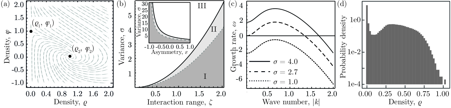
We begin our analysis of the stability conditions of Eq. (4) by considering a system composed of a single component, $\rho$, and a constant potential $V$. We will later discuss the role of non-constant local potentials in conservative processes. Eq. (4) then admits two spatially homogeneous stationary solutions: $\left(\rho^{*}_{1},\phi^{*}_{1}\right)=\left(0,h^{0}\right)$ is stable if the local birth-death process is subcritical, $h^{0}<0$, and unstable otherwise. The fixed point $\left(\rho^{*}_{2},\phi^{*}_{2}\right)=\left(h^{0}/(\zeta h^{1}),0\right)$ exists only if $h^{0}>0$ and it is stable [Fig. 2(a)]. The feedback with the field $\phi$ prevents the unbounded growth of the density even for supercritical birth-death processes.

The stability of these states with respect to spatiotemporal perturbations of the density $\rho$ can be assessed within the framework of linear stability analysis. This implies linearizing Eq. (4) around the stationary states, $\rho(\vec{z},t)=\rho_{1,2}^{*}+\delta\rho(\vec{z},t)$, and studying the response of the linearized system to spatially inhomogeneous perturbations. This procedure yields a dispersion relation between the growth rate $\omega$ and the wave vector $\vec{k}$ of a spatially periodic perturbation. If the maximum of $\omega$ is positive and occurs at a finite value of $|\vec{k}|$, linear stability analysis predicts the emergence of a pattern with a finite length scale. For single-component systems, $w$ is never positive for finite values of $|\vec{k}|$, and such systems therefore do not show pattern formation. These results are consistent with a structurally similar model that has been studied in the context of stem cells in spermatogenesis [22].

For systems comprising multiple components, the stability of stationary states may be altered by interactions between different components. In order to investigate the stability of the multi-component system, Eq. (4), we will first derive a phase diagram for the stability of the homogeneous stationary solutions to global perturbations. In the second step, we will then study spatiotemporal patterns in each regime. To this end, following Ref. [1], we take $K_{ij}$ to be Gaussian distributed with mean $0$, variance $\sigma^{2}/L$ and covariance $\epsilon\sigma^{2}/L$ ¹¹1With this choice, at each position $\vec{z}$ the dynamics of Eq. (4) resembles that of a soft spin glass..

Following Ref. [29, 30, 31] we use a path integral representation of Eq. (4) and perform the average over all realizations of $K_{ij}$. Within this formulation, in the limit of large $L$, we express the interaction between components in terms of a coupling to an effective response function, $\chi_{i}(t,t^{\prime},\vec{z},\vec{z^{\prime}})$, and Gaussian colored noise, $W_{i}$. This reduces the $2L$ coupled equations, Eq. (4), to $L$ uncoupled equations,

	$\displaystyle\partial_{t}\rho_{i}=$	$\displaystyle\mathcal{L}\left[\rho_{i}\right]+\epsilon\sigma^{2}\rho_{i}\int_{0}^{t}\text{d}t^{\prime}\int\text{d}\vec{z}^{\prime}\chi_{i}(t,t^{\prime},\vec{z},\vec{z}^{\prime})\rho_{i}(\vec{z}^{\prime},t^{\prime})$
		$\displaystyle+W_{i}\rho_{i}+\eta_{i}+\divergence\vec{\xi_{i}}\,.$		(5)

In Eq. (5), $W_{i}$ has zero mean and its correlations are proportional to the correlations of the fields ($C_{i,j}(\vec{z},\vec{z}^{\prime},t,t^{\prime})=\langle\rho_{i}(\vec{z},t)\rho_{j}(\vec{z}^{\prime},t^{\prime})\rangle$) such that $\langle W_{i}(\vec{z},t)W_{j}(\vec{z}^{\prime},t^{\prime})\rangle=\sigma^{2}\delta(t-t^{\prime})\delta_{i,j}C_{i,j}(\vec{z},\vec{z}^{\prime},t,t^{\prime})$ and the response function $\chi_{i}(\vec{z},\vec{z}^{\prime},t,t^{\prime})=\langle\partial\rho_{i}(\vec{z},t)/\partial W_{i}(\vec{z^{\prime}},t^{\prime})|_{W_{i}=0}\rangle$ [29, 30]. In a spatially homogeneous stationary state of Eq. (5), $\rho_{i}^{*}$, the response and correlation functions are time-independent, such that we define $\int\text{d}t^{\prime}\,\chi_{i}(t,t^{\prime})\equiv\chi_{i}^{*}$ and $C_{i}(t,t^{\prime})=\langle\rho_{i}^{*2}\rangle\equiv c_{i}$. The stationary value of the noise is $W_{i}^{*}=\sqrt{\sigma^{2}c_{i}}w$ [32, 33], where $w$ is a Gaussian random variable with unitary variance and zero mean.

In order to find stationary solutions of Eq. (5) we take the mean-field limit where multiplicative noise contributions coming from density fluctuations and birth-death processes are negligible, which in our system is not expected to change the stationary states [7]. As $W_{i}$ describes the effect of deterministic interactions between different components in Eq. (4) it can not be neglected in the mean-field limit. There are two homogeneous solutions of Eq. (5), given by the random variables $(\rho_{1}^{*},\phi_{1}^{*})=(0,h^{0}/\alpha)$ and

$$\rho^{*}_{2}=\frac{w\sigma\sqrt{c}+h^{0}}{\Delta(\chi^{*})}\Theta\left(\ \frac{w\sigma\sqrt{c}+h^{0}}{\Delta(\chi^{*})}\right)$$

(6)

where we assumed equal parameter values for all components and consequently dropped the index $i$. $\Theta(x)$ is the Heaviside step function and we defined $\Delta(\chi^{*})\equiv h^{1}\zeta-\epsilon\sigma^{2}\chi^{*}$. With $\rho^{*}_{2}$ defined the value of $\phi^{*}_{2}$ then follows from Eq. (2). As $w$ is a Gaussian random variable the density in the stationary state, $\rho_{2}^{*}$, follows a Gaussian distribution truncated at $0$. Therefore, as expected, the strength of particle production processes sets the mean of the stationary particle density distributions and the variance of the distribution is proportional to the variance of interactions between components.

In order to obtain an expression for the parameters of the distribution of $\rho_{2}^{*}$, Eq. (6), we derive self-consistency equations for its moments: the stationary value of the fraction of surviving components, $f_{s}$, the average density of particles, $M^{*}=\langle\rho^{*}\rangle$, the response function $\chi^{*}$, and the correlation function, $c$. The self-consistency equations read

$$\begin{split}f_{s}=\int_{-\kappa}^{\infty}\text{D}w\,,\;M^{*}&=\frac{\alpha\sigma\sqrt{c}}{\Delta(\chi^{*})}\int_{-\kappa}^{\infty}\text{D}w\left(w+\kappa\right)\,,\\ \chi^{*}=\frac{\alpha}{\Delta(\chi^{*})}\int_{-\kappa}^{\infty}\text{D}w,\;1&=\frac{\alpha^{2}\sigma^{2}}{\Delta(\chi^{*})^{2}}\int_{-\kappa}^{\infty}\text{D}w\left(w+\kappa\right)^{2}.\end{split}$$

(7)

Here we defined $\text{D}w\equiv\text{d}w\,e^{-w^{2}/2}/\sqrt{2\pi}$ and $\kappa\equiv h^{0}/\left(\sigma\sqrt{c}\right)$ is a threshold value of $w$ above which the density $\rho_{2}^{*}$ is a possible solution of Eq. (5). Eq. (7) can be solved numerically.

Global instability of the stationary states is associated with diverging correlations in density fluctuations, $\tilde{C}\equiv\langle\delta\rho(\vec{z},t)\delta\rho(\vec{z}\,^{\prime},t^{\prime})\rangle$ where $\delta\rho=\rho-\rho_{2}^{*}$ [32, 31]. In order to determine the conditions under which correlation functions diverge, we linearize Eq. (5) around the homogeneous stationary state $\rho_{2}^{*}$ and express two-point spatiotemporal correlation functions in Fourier space,

$\displaystyle\tilde{C}(\vec{k},\vec{k}^{\prime},\omega,\omega^{\prime})=\frac{\Lambda(\vec{k})\delta(\vec{k}+\vec{k}^{\prime})\delta(\omega+\omega^{\prime})}{\big{\langle}\absolutevalue{\frac{i\omega}{\rho^{*}}-\Omega(\vec{k},\omega)}^{-2}\big{\rangle}_{+}^{\!-1}-f_{s}\sigma^{2}}\,,$

(8)

where we defined $\Lambda(\vec{k})=f_{s}(h^{0}/\alpha+2Dk^{2})\langle\rho^{*}\rangle_{+}$ and $\Omega(\vec{k},\omega)=-\left(\frac{D}{\rho^{*}}\vec{k}^{2}+\frac{h^{1}\zeta}{1+\zeta^{2}\vec{k}^{2}}\right)+\epsilon\sigma^{2}\chi(\vec{k},\omega)\,.$ $\langle\dots\rangle_{+}$ denotes the average over the positive fraction of surviving components $f_{s}$ [32].

The correlation functions Eq. (8) of the stationary homogeneous state, $\omega\to 0$ and $|\vec{k}|\to 0$, diverge if $\Omega(0,0)^{2}=f_{s}\sigma^{2}$. This condition can be satisfied only if $h_{0}\geq 0$. Substituting $\Omega(0,0)^{2}=f_{s}\sigma^{2}$ into Eq. (7) gives the critical value of the variance of interaction strengths below which the system is stable with respect to homogeneous perturbations [dashed line in Fig. 2(b)],

$$\sigma_{c}={\sqrt{2}h^{1}\zeta}/{(1+\epsilon)}\,.$$

(9)

Therefore, non-local birth-death processes globally stabilize the system. By contrast, the degree of symmetry in interactions between components, $\epsilon$, destabilizes the homogeneous state. For anti-symmetric interactions, $\epsilon=-1$, the system is always stable. Therefore, predator-prey interactions stabilize ecosystems against global perturbations. If $h^{0}<0$ extinction is the only stable fixed point such that interactions between components do not affect the stability to linear order.

In order to further characterize the instability we now investigate whether the stable, homogeneous solutions can be destabilized by spatial perturbations in the regime where $\sigma<\sigma_{c}$. For stochastic systems, pattern formation is reflected in a finite-wavelength peak of the spectral density functions in the long-term limit, $\langle|\delta\rho(\vec{k},0)|^{2}\rangle$ [34, 35]. The onset of a pattern instability follows from solving $\divergence C(\vec{k},0)|_{\vec{k}^{*}}=0$ for $\vec{k}$ and $C(\vec{k},0)|_{\vec{k}^{*}}=0$. Analytical solutions to this equation are feasible in the long-term limit, $\omega\rightarrow 0$, and using the approximation that averages of functions of the fields equal the functions of averages. Following Refs. [32, 36] then yields a criterion the instability of Eq. (4) with respect to spatial perturbations.

The condition for pattern instability also follows from random-matrix theory [37, 31], requiring that the largest eigenvalue describing the relaxation of a perturbation of Eq. (4) around a stable homogeneous state is positive at a finite value of $|\vec{k}|$. This yields

$$-h^{1}\zeta/(1+\zeta^{2}\vec{k}^{2})-D\vec{k}^{2}/M^{*}+\sqrt{f_{s}}\sigma(1+\epsilon)>0\,,$$

(10)

and it is convex at that value [Fig. 2(c)]. We find that a pattern instability is possible if $\sigma_{p}<\sigma<\sigma_{c}$ with a critical threshold $\sigma_{p}$ given by $\sigma_{p}=\sigma_{c}/\sqrt{2}$. Notably, the regime exhibiting pattern formation is fully determined by $\sigma_{c}$ and otherwise independent of the model parameters. $\sigma_{c}$ and $\sigma_{p}$ could be decoupled for models involving component-dependent dispersal [5] or higher order interactions [38] .

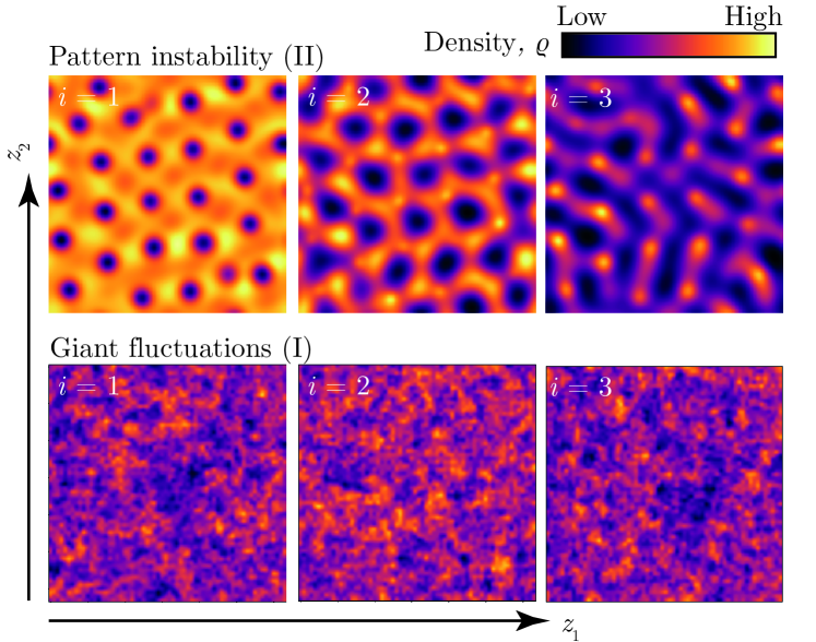
Figure 3 shows numerical solutions of Eq. (4) in the pattern forming regime. Although individual components exhibit different patterns, they occur with an identical length scale. Indeed, Eq. (5) implies that the dynamics of individual components are effectively coupled via a shared response function.

Although the system is stable against homogeneous and spatial perturbations for $\sigma<\sigma_{p}$ the presence of intrinsic noise can lead to the extinction of all components. In order to characterize the risk of extinction, we investigate fluctuations around the stationary state $(\rho_{2}^{*},\phi_{2}^{*})$ in this regime. In the limit of $|\vec{k}|\to\infty$ and $\omega\to 0$, Eq (8) shows an algebraic decay following $|\vec{k}|^{-2}$. This is a hallmark of giant-density fluctuations [39, 40], whose strength in a given subsystem scales stronger than predicted by the central limit theorem. These giant-density fluctuations are also reflected in finite difference simulations of Eq. (4), cf. Fig. 2(d) and Fig. 3. Therefore, multiplicative noise from microscopic processes leads to strong fluctuations and an increased risk of extinction in the stable regime.

Taken together, we generalized the May bound for the stability of complex systems [1] to features characteristic of biological systems: strong, multiplicative noise stemming from small copy numbers and non-local interactions, which are often mediated by diffusing signaling factors. Starting from a microscopic model definition we derived an effective field theory. We showed that non-local interactions and multiplicative noise both alter the conditions for stability with respect to the May bound. In particular, multiplicative noise stemming from non-conservative processes gives rise to giant density fluctuations in stable stationary states whilst conservative processes could potentially destabilize the stable region of the phase space giving rise to the formation of spatial patterns. By extending the theory by non-local conservative terms or vectorial fields our work can be applied to other systems such as multi-component phase separation or active matter.

References

- May [1972] R. M. May, Will a large complex system be stable?, Nature 238, 413 (1972).
- Wigner [1958] E. P. Wigner, On the distribution of the roots of certain symmetric matrices, Annals of Mathematics 67, 325 (1958).
- Allesina and Tang [2012] S. Allesina and S. Tang, Stability criteria for complex ecosystems, Nature 483, 205 (2012).
- Knebel et al. [2013] J. Knebel, T. Krüger, M. F. Weber, and E. Frey, Coexistence and survival in conservative lotka-volterra networks, Phys. Rev. Lett. 110, 168106 (2013).
- Baron and Galla [2020] J. W. Baron and T. Galla, Dispersal-induced instability in complex ecosystems, Nature communications 11, 1 (2020).
- Bunin [2017] G. Bunin, Ecological communities with lotka-volterra dynamics, Phys. Rev. E 95, 042414 (2017).
- Biroli et al. [2018] G. Biroli, G. Bunin, and C. Cammarota, Marginally stable equilibria in critical ecosystems, New Journal of Physics 20, 083051 (2018).
- Geiger et al. [2018] P. M. Geiger, J. Knebel, and E. Frey, Topologically robust zero-sum games and pfaffian orientation: How network topology determines the long-time dynamics of the antisymmetric lotka-volterra equation, Phys. Rev. E 98, 062316 (2018).
- Knebel et al. [2015] J. Knebel, M. F. Weber, T. Krüger, and E. Frey, Evolutionary games of condensates in coupled birth–death processes, Nature communications 6, 1 (2015).
- Pigolotti et al. [2010] S. Pigolotti, C. López, E. Hernández-García, and K. H. Andersen, How gaussian competition leads to lumpy or uniform species distributions, Theoretical Ecology 3, 89 (2010).
- Hu et al. [2022] J. Hu, D. R. Amor, M. Barbier, G. Bunin, and J. Gore, Emergent phases of ecological diversity and dynamics mapped in microcosms, Science 378, 85 (2022).
- Schimansky-Geier et al. [2003] L. Schimansky-Geier, D. Abbott, A. Neiman, C. Van den Broeck, et al., Noise in complex systems and stochastic dynamics (SPIE, 2003).
- Biancalani et al. [2017a] T. Biancalani, F. Jafarpour, and N. Goldenfeld, Giant amplification of noise in fluctuation-induced pattern formation, Phys. Rev. Lett. 118, 018101 (2017a).
- Hutt [2008] A. Hutt, Additive noise may change the stability of nonlinear systems, EPL (Europhysics Letters) 84, 34003 (2008).
- García-Ojalvo and Sancho [1999] J. García-Ojalvo and J. M. Sancho, Noise in spatially extended systems (1999).
- Fogler and Fogler [1999] H. S. Fogler and S. H. Fogler, Elements of chemical reaction engineering (Pearson Educacion, 1999).
- Göppel et al. [2016] T. Göppel, V. V. Palyulin, and U. Gerland, The efficiency of driving chemical reactions by a physical non-equilibrium is kinetically controlled, Physical Chemistry Chemical Physics 18, 20135 (2016).
- Volterra [1928] V. Volterra, Variations and fluctuations of the number of individuals in animal species living together, ICES Journal of Marine Science 3, 3 (1928).
- Lotka [1920] A. J. Lotka, Analytical note on certain rhythmic relations in organic systems, Proceedings of the National Academy of Sciences 6, 410 (1920).
- Cates and Tailleur [2013] M. E. Cates and J. Tailleur, When are active brownian particles and run-and-tumble particles equivalent? consequences for motility-induced phase separation, EPL (Europhysics Letters) 101, 20010 (2013).
- Kampen [2007] N. V. Kampen, Stochastic processes in physics and chemistry (North Holland, 2007).
- Jörg et al. [2021] D. J. Jörg, Y. Kitadate, S. Yoshida, and B. D. Simons, Stem cell populations as self-renewing many-particle systems, Annual Review of Condensed Matter Physics 12, 135–153 (2021).
- Robertson and Skeldon [2007] N. Robertson and A. Skeldon, Patterns in a non-local reaction diffusion equation (2007).
- Mobilia et al. [2007] M. Mobilia, I. T. Georgiev, and U. C. Täuber, Phase transitions and spatio-temporal fluctuations in stochastic lattice lotka–volterra models, Journal of Statistical Physics 128, 447 (2007).
- Dean [1996] D. S. Dean, Langevin equation for the density of a system of interacting langevin processes, Journal of Physics A: Mathematical and General 29, L613–L617 (1996).
- Kawasaki and Koga [1993] K. Kawasaki and T. Koga, Relaxation and growth of concentration fluctuations in binary fluids and polymer blends, Physica A: Statistical Mechanics and its Applications 201, 115–128 (1993).
- Chavanis [2019] P.-H. Chavanis, The generalized stochastic smoluchowski equation, Entropy 21, 1006 (2019).
- Note [1] With this choice, at each position the dynamics of Eq. (4) resembles that of a soft spin glass.
- Sompolinsky and Zippelius [1982] H. Sompolinsky and A. Zippelius, Relaxational dynamics of the edwards-anderson model and the mean-field theory of spin-glasses, Phys. Rev. B 25, 6860 (1982).
- Kirkpatrick and Thirumalai [1987] T. R. Kirkpatrick and D. Thirumalai, p-spin-interaction spin-glass models: Connections with the structural glass problem, Phys. Rev. B 36, 5388 (1987).
- Galla [2018] T. Galla, Dynamically evolved community size and stability of random lotka-volterra ecosystems (a), EPL (Europhysics Letters) 123, 48004 (2018).
- Opper and Diederich [1992] M. Opper and S. Diederich, Phase transition and 1/f noise in a game dynamical model, Phys. Rev. Lett. 69, 1616 (1992).
- Biscari and Parisi [1995] P. Biscari and G. Parisi, Replica symmetry breaking in the random replicant model, Journal of Physics A: Mathematical and General 28, 4697–4708 (1995).
- Biancalani et al. [2017b] T. Biancalani, F. Jafarpour, and N. Goldenfeld, Giant amplification of noise in fluctuation-induced pattern formation, Phys. Rev. Lett. 118, 018101 (2017b).
- Hernández-Garc´ıa and López [2004] E. Hernández-García and C. López, Clustering, advection, and patterns in a model of population dynamics with neighborhood-dependent rates, Physical Review E 70, 016216 (2004).
- Roy et al. [2019] F. Roy, G. Biroli, G. Bunin, and C. Cammarota, Numerical implementation of dynamical mean field theory for disordered systems: application to the lotka–volterra model of ecosystems, Journal of Physics A: Mathematical and Theoretical 52, 484001 (2019).
- Sommers et al. [1988] H. J. Sommers, A. Crisanti, H. Sompolinsky, and Y. Stein, Spectrum of large random asymmetric matrices, Phys. Rev. Lett. 60, 1895 (1988).
- Sidhom and Galla [2020] L. Sidhom and T. Galla, Ecological communities from random generalized lotka-volterra dynamics with nonlinear feedback, Phys. Rev. E 101, 032101 (2020).
- Houchmandzadeh [2009] B. Houchmandzadeh, Theory of neutral clustering for growing populations, Phys. Rev. E 80, 051920 (2009).
- Houchmandzadeh [2002] B. Houchmandzadeh, Clustering of diffusing organisms, Phys. Rev. E 66, 052902 (2002).