Long-term 4.6m Variability in Brown Dwarfs and a New Technique for Identifying Brown Dwarf Binary Candidates
Abstract
Using a sample of 361 nearby brown dwarfs, we have searched for 4.6m variability indicative of large-scale rotational modulations or large-scale long-term changes on timescales of over 10 years. Our findings show no statistically significant variability in Spitzer ch2 or WISE W2 photometry. For Spitzer the ch2 1 limits are 8 mmag for objects at 11.5 mag and 22 mmag for objects at 16 mag. This corresponds to no variability above 4.5 at 11.5 mag and 12.5 at 16 mag. We conclude that highly variable brown dwarfs, at least two previously published examples of which have been shown to have 4.6m variability above 80 mmag, are very rare. While analyzing the data, we also developed a new technique for identifying brown dwarfs binary candidates in Spitzer data. We find that known binaries have IRAC ch2 PRF (point response function) flux measurements that are consistently dimmer than aperture flux measurements. We have identified 59 objects that exhibit such PRF versus apertures flux differences and are thus excellent binary brown dwarf candidates.
1 Introduction
Brown dwarfs have similar chemical composition and size to large gaseous planets, indicating that brown dwarfs have the potential for cloud bands and large surface storms, like that of the Great Red Spot on Jupiter. It has been found that some brown dwarfs exhibit variability over short periods of a couple of hours to a few days, first reported in Bailer-Jones & Mundt (1999) and Kolb & Baraffe (1999). Artigau et al. (2009) and Yang et al. (2016) found variability as high as 14-420 mmag, mostly in the , , and bands over several rotational periods. This is a result of inhomogeneities in the brown dwarf’s cloud bands or local storms, which induces observed variability as the object rotates. However, none of these papers explore long-term variability over timescales of years. Additionally, we might expect stellar flares in the warmest brown dwarfs as a result of their similarities to low-mass stars (Gizis et al. 2017, Ducrot et al. 2020).
The goal of this paper is to examine long-term variability, on years to decade timescales, at 4.6m for a large brown dwarf sample. This would not only be sensitive to rotationally modulated variability due to inhomogeneity over the surface, but would also be sensitive to long-term global changes in the atmosphere.
While examining variability, we developed a new technique for identifying brown dwarf binary candidates in Spitzer data. Our Spitzer reductions measure both the aperture and point response function-fit (hereafter, PRF-fit) fluxes. If the PRF-fit fluxes are consistently dimmer than the aperture measurements, then it may be indicative of a binary brown dwarf system. We demonstrate this with known binaries and background-contaminated objects.
In §2 we discuss expectations of variability based on previous research. We then discuss the data acquisition and reduction in §3 and its analysis in §4. Long-term variability is explored in §5, while the new technique for discovering brown dwarf binary candidates is discussed in §6. The results from these two sections are then compared to what was previously known about brown dwarf variability and binarity in §7.
2 Variability Expectations
Most previous papers on brown dwarf variability have focused on hemisphere-to-hemisphere inhomogeneity. As a result of brown dwarfs having a range of rotational periods from about an hour to a few weeks (Tannock et al. 2021, Luhman 2012), these studies have only concentrated on a few-day to few-week timescale. Some of these studies have repeated this analysis on return trips to look for anomalies on the surface of brown dwarfs that might change many rotational periods in the future (Apai et al. 2017).
Studies such as Kellogg et al. (2017), Radigan et al. (2012), Radigan et al. (2014a), and Radigan (2014b) between 0.9-2.5m and Vos et al. (2022) and Yang et al. (2016) between 3.6-4.5m found variability in the L/T dwarf transition but did not sample the entire brown dwarf spectral range. Additional studies (Metchev et al. 2015 and Cushing et al. 2016) found that large variations of >2 in Spitzer/IRAC ch1 (3.6m) and ch2 (4.5m) exist across L/T/Y spectral types. It has been shown that large variations occur in the (1.25m) and / (2.2m) bands, sometimes as large as 420mmag in (Artigau et al. 2009). Studies at r-band (0.658m) for M and L dwarfs found that 50 vary at a level of >2 (Artigau 2018).
Brown dwarf variability is believed to be caused by a variety of different physical phenomena. The most explored and discussed explanation is that brown dwarfs have a mixture of dusty clouds and hazes (e.g. Marley et al. 2013 and Tsuji 2005). SIMP J013656.57+093347.3 is believed to have 75 of its surface covered by dusty clouds based on its to variability ratio, (Artigau et al. 2009). An alternative idea is that variability is caused by differentially rotating cloud bands. Some cloud bands may appear more optically thin, depending on the filter used. This idea is explored in Yang et al. (2016), where six brown dwarfs were observed to have variability on the scale of a few percent. This variability was linked to differential cloud rotation and atmospheric optical depth, causing inhomogeneities in longitude.
Another scenario is local storms that can be seen on the top of an object’s atmosphere, similar to the Great Red Spot on Jupiter. Jupiter and brown dwarfs have been juxtaposed multiple times throughout the history of brown dwarfs studies. Gelino & Marley (2000) explore the similarities that the gas giants of our solar system could have with brown dwarfs. As a storm rotates or increases/decreases in size, it could lead to variability seen in an unresolved disk. Gelino & Marley (2000) predicted that an unresolved storm similar to Jupiter’s Great Red Spot would create variability on the order of 0.2 mag at 4.78m but only 0.04 mag at 0.410m. Ge et al. (2019) found that Jupiter exhibits peak-to-peak variability upwards of 20 at 5m, which is where this variability is the greatest, indicating that brown dwarfs may exhibit such behavior and that using the WISE W2 band would be an excellent band in which to search for such variability in brown dwarfs.
Our study uses a different approach than previous studies of brown dwarf variability, such as Metchev et al. (2015) who used Spitzer/IRAC’s sweet spot for which corrections for the pixel phase effect (Deming et al. 2015) enables extremely high levels of photometric precision. Such studies are thus sensitive to small amplitude variability (>0.2 for 3 to 5m) at short timescales (typically <20 hours). While studies of variability over longer time baselines of several months have been performed (e.g., Yang et al. 2016), an investigation of substellar object variability over several year time baselines has yet to be attempted. Because our observations are randomly sampled over several years, we expect significant coverage of all hemispheres, allowing for an investigation of large-amplitude variability.
3 Photometry
3.1 Spitzer/IRAC Channel 2
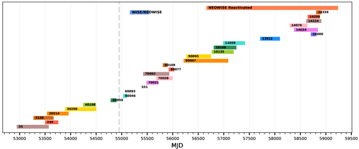
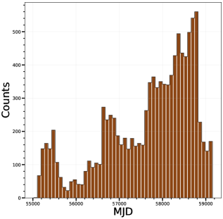
The photometry used in this work is derived from the Spitzer observations (IRSA 2022) used to compute the trigonometric parallaxes of 361 L, T, and Y dwarfs in Kirkpatrick et al. (2021), covering a long time baseline (Figure 1). This long time baseline, spanning upwards of seventeen years, provides an excellent dataset with which to study brown dwarfs at their peak wavelengths over a timescale that has never been explored before. The photometry comes from Spitzer’s Infrared Array Camera (hereafter, Spitzer/IRAC; Fazio et al. 2004), which, during the cryogenic mission, was capable of observing at ch1 (3.6m), ch2 (4.6m), ch3 (5.8m), and ch4 (8.0m) bands (Werner et al. 2004). Of these four, the one that was used is Spitzer ch2, as this is the band in which brown dwarfs are brightest (Mainzer et al. 2011).
Spitzer’s cryogenic mission observed only 14 of the 361 objects in our sample. However, every object includes Spitzer warm mission ch2 data, and most have a time baseline of >10 years.
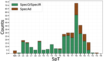
The spectral type distribution for these 361 brown dwarfs is seen in Figure 2. These spectral types come from Kirkpatrick et al. (2021) where objects that have optical and infrared spectra are marked as “SpecO/SpecIR” and objects that have spectral classifications based on colors are marked with “SpecAd”.
Most objects are at distances <20pc, which makes them the brightest members of their class. Hence, the photometric uncertainties will be as low as possible, allowing us the best chance to detect variability for these classes. Moreover, the majority of these objects were observed for several years and multiple times a year, meaning that each object will have an abundance of data points.
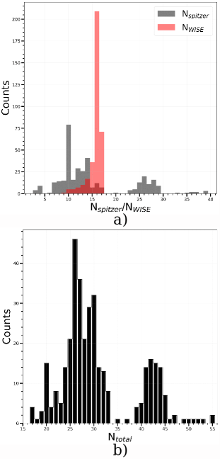
Figure 3a shows the number of Astronomical Observation Requests (hereafter, AOR), Nspitzer, for all 361 objects. Most objects have 6-16 AORs. However, many objects have >16 AORs and these will have the most data-rich light curves.
3.2 WISE W2
To provide additional 4.6m data, NASA’s Wide-field Infrared Survey Explorer (hereafter, WISE; Wright et al. 2010) and Near-Earth Object WISE (hereafter, NEOWISE; Mainzer et al. 2011) W2 photometry was considered. As Figure 15 of Kirkpatrick et al. (2021) shows, Spitzer ch2 and WISE W2 filter bandpasses for brown dwarfs can be interchanged. WISE data were obtained by cross-matching our objects with the unTimely Catalog (Meisner et al. 2022), which contains detections from WISE/NEOWISE W2 coadds. The unTimely Catalog contains time-series W1 and W2 photometry from the beginning of the WISE mission to the most current publicly released NEOWISE data. The WISE and NEOWISE timescales can be seen at the top of Figure 1. The unTimely Catalog also contains W1 photometry over multiple epochs; this photometry could be explored for variability in future research.
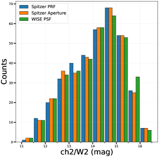
Figure 3a shows the distribution of the number of unTimely detections, NWISE, per object. There is much less variation compared to Nspitzer as a result of WISE/NEOWISE covering the whole sky every six months. Theoretically, every object should have 16 unTimely detections for each of the 16 sky passes made from classic WISE up through NEOWISE year 7. However, some objects have NWISE values of <16 because of background contamination problems. Due to the fact that the WISE spacecraft precesses, some objects will have NWISE values of 17 because in NEOWISE year 7 a portion of the sky already has its 17th coverage. The distribution of the number of points per object, combining Nspitzer and NWISE, can be seen in Figure 3b. Figure 4 displays the distribution for each photometry measurement per magnitude interval. Lastly, Figure 5 shows the distribution of Spitzer and unTimely points per MJD interval. We can see that the number of points per unit time increases with time.
4 Understanding the Photometry
An object’s median Spitzer ch2 flux and its standard deviation were calculated for a single AOR by taking the median of the measured flux in all the dithers for that particular AOR. The magnitudes were calculated using these formulas:
| (1) |
| (2) |
where ch2aperture is the aperture magnitude, ch2PRF is the PRF-fit magnitude, F0 is the flux at zero magnitude (179700000 Jy, Table 4.2 of the Spitzer/IRAC Handbook111https://irsa.ipac.caltech.edu/data/SPITZER/docs/irac/iracinstrumenthandbook/IRAC_Instrument_Handbook.pdf), Fap is the measured aperture flux in Jy from the MOPEX/APEX output (described below), FPRF is the measured PRF-fit flux in Jy from the same output, Cap is the aperture correction (Table 4.8 of the Spitzer/IRAC Handbook), and CPRF is the PRF-fit correction (Table C.1 of the Spitzer/IRAC Handbook). This median technique was done to help us mitigate dithers that were affected by cosmic ray hits.
For the unTimely data points, the only measurement that is offered in the catalog is a Point Spread Function-fit (hereafter, PSF-fit; Schlafly et al. 2019), which is analogous to the Spitzer PRF-fit. Flux measurements were obtained directly from the catalog because Schlafly, Meisner, & Green (2019) calculated the flux and its uncertainties within the code. The magnitudes and their uncertainties were calculated using the formula: magWISE = (Schlafly, Meisner, & Green 2019).
Our Spitzer ch2 data were reduced in Kirkpatrick et al. (2021) using the MOPEX/APEX code (Makovoz et al. 2006). Aperture photometry counts all the flux within a circle of fixed radius. For this study, the aperture radius used is . For background subtraction, the flux in a concentric annulus is medianed, and that value is subtracted off the aperture measurement to reveal the true target flux. The annulus has an inner radius of and an outer radius of (Spitzer/IRAC Handbook222https://irsa.ipac.caltech.edu/data/SPITZER/docs/irac/iracinstrumenthandbook/IRAC_Instrument_Handbook.pdf). The second photometry method is to perform a PRF fit (Hora et al. 2012), which approximates the 3 parameter (x, y, and flux) distribution of our target flux to a known 3 parameter shape of a point source. The aperture and PRF-fit measurements were used to verify any variability seen, because if a variable point is seen in both measurements, it suggests that it is real and not an artifact of processing. For example, the aperture measurement is susceptible to cosmic ray hits, while the PRF-fit photometry ideally can remove this contamination.
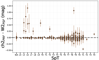
To further test the consistency of the Spitzer PRF-fit ch2 measurements with those of the unTimely PSF-fit, we plotted the difference between the average ch2PRF and the average W2PSF for each object. This is plotted against spectral type in Figure 6. The trend hovers around 0 for objects before T8, which supports the compatibility of the Spitzer/IRAC ch2 magnitudes and the WISE/unTimely W2 magnitudes. Objects later than T8 have a considerable amount of scatter as a result of these objects having poor S/N in W2. Outliers earlier than spectral type T8 on this plot are a result of blending in Spitzer or WISE caused by background contamination or possibly binarity, as further discussed in §6.
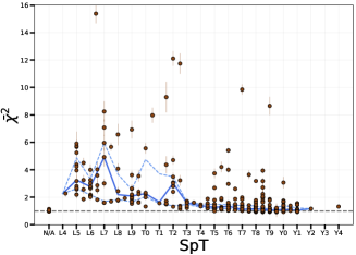
An important statistic to consider is the value for the Spitzer PRF-fit. The cause of a high is that the MOPEX ch2 PRF was a poor fit to the data. In Figure 7 we compare spectral type to the averaged value. The object’s AOR value was calculated by performing a weighted average of all the dithers, and then the overall was computed using a weighted average of all the AORs (the weight for these averages are the inverse variance for the photometry). The solid blue line in Figure 7 is the median for each spectral type, with the dashed light blue lines showing the lower and upper quartiles Q1 (25) and Q3 (75). Outliers are discussed further in §6.
5 Variability Results
Now that the photometry has been analyzed, we can discuss our definition of variability. To formally define variability, we require that there are points lying >3 away from the median value. A 3 requirement means that we would expect only one object in a sample of 361 independent objects to show such an excursion by chance. This >3 requirement searches for variability for each photometry type separately: ch2aperture, ch2PRF, and W2PSF. We found that 24 of our 361 objects have such variability.
| Object Name | RA (Deg) | Dec (Deg) | Dataset | Note |
|---|---|---|---|---|
| WISE J003110.04+574936.3 | 7.79433 | 57.826773 | W2PSF | Blended with Background Source |
| WISE J003231.09494651.4 | 8.128736 | 49.782059 | W2PSF | Blended with Background Source |
| WISEP J015010.86+382724.3 | 27.546953 | 38.456528 | W2PSF | Blended with Background Source |
| WISEPA J031325.96+780744.2 | 48.359129 | 78.129099 | ch2PRF | Blended with Background Source |
| WISE J032504.33504400.3 | 51.268182 | 50.733501 | W2PSF | Blended with Background Source |
| SDSSp J033035.13002534.5 | 52.64629 | 0.42628 | W2PSF | Blended with Background Source |
| 2MASS J042107186306022 | 65.281665 | 63.099437 | W2PSF | Blended with Background Source |
| WISE J064723.23623235.5 | 101.84721 | 62.542746 | ch2PRF | Cosmic Ray Affects 1 Epoch |
| WISE J071322.55291751.9 | 108.34441 | 29.298264 | W2PSF | Blended with Background Source |
| WISE J103907.73160002.9 | 159.78173 | 16.001139 | ch2PRF | Cosmic Ray Affects 1 Epoch |
| WISE J112438.12042149.7 | 171.15781 | 4.363732 | W2PSF | Blended with Background Source |
| WISEA J114156.67332635.5 | 175.48445 | 33.443475 | ch2PRF/W2PSF | Blended with Background Source |
| WISEPC J151906.64+700931.5 | 229.77879 | 70.157919 | ch2PRF/W2PSF | Blended with Background Source |
| CWISEP J160835.01244244.7 | 242.14633 | 24.712494 | W2PSF | Blended with Background Source |
| WISEPA J171104.60+350036.8 | 257.76888 | 35.010238 | ch2PRF | Cosmic Ray Affects 1 Epoch |
| WISE J174303.71+421150.0 | 265.76558 | 42.196369 | W2PSF | Blended with Background Source |
| WISE J192841.35+235604.9 | 292.17202 | 23.93489 | ch2PRF | Blended with Background Source |
| WISE J195500.42254013.9 | 298.7526 | 25.671162 | ch2PRF | Cosmic Ray Affects 1 Epoch |
| WISEPA J195905.66333833.7 | 299.77339 | 33.642956 | ch2aperture | Cosmic Ray Affects 1 Epoch |
| WISE J201546.27+664645.1 | 303.94207 | 66.779688 | ch2PRF | Blended with Background Source |
| CWISEP J210007.87293139.8 | 315.03349 | 29.52782 | W2PSF | Blended with Background Source |
| WISEPA J231336.40803700.3 | 348.40273 | 80.616879 | ch2PRF | Blended with Background Source |
| WISE J235716.49+122741.8 | 359.31997 | 12.459123 | ch2aperture | Cosmic Ray Affects 1 Epoch |
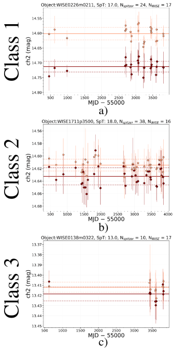
We found that the variability for all 24 objects is a result of a non-physical property of the brown dwarf. All 24 objects are listed in Table 1. The most common cause of W2PSF variability is contamination from a background source that the object was blended with in one or more epochs. All objects with ch2aperture variability have a single AOR that is bombarded with cosmic ray hits in all but a few dithers. With all 24 objects being labeled as false, we find 0 out of 361 objects with true long-term variability. We further discuss this result in §7.1. The complete figure set of light curves (361 images) is available in the online journal. An example from this figure set can be seen in Figure 8.
Fig. Set8. Light curves for the 361 objects
6 New Technique for Identifying Binary Brown Dwarf Candidates
As discussed in §4 we use two different types of flux measurements for the Spitzer ch2 photometry, both aperture and PRF-fit. A disadvantage of the aperture magnitude is that it can become cross contaminated from a secondary component, background source, or cosmic ray hit. The Spitzer ch2 PRF-fit code, on the other hand, can attempt to fit the secondary, remove the background source, or ignore the cosmic ray to better estimate the true apparent magnitude for the object. However, the PRF-fit magnitude can be biased if the object is a partly resolved physical binary (within the MOPEX FWHM; later discussed in §7.2) or a blend with a distant stellar object or extragalactic source.
Our binary identification technique is a close variant of the widely used star-galaxy separation technique that interprets an excess of aperture flux relative to PSF flux as an indication of resolved rather than pointlike morphology. Such an approach has been used by major optical surveys, including Pan-STARRS (e.g., Schlafly et al. 2012).
Within Spitzer’s ch2 PRF fitting code, there is a procedure called “passive deblending”, in which the code tries to separate what is believed to be two, or more, sources and then tries to fit multiple PRFs to the detection (Makovoz & Marleau 2005). Once multiple PRFs are fit to the detection, those are subtracted to get uncertainties, , and the S/N to compare to a single PRF-fit. MOPEX then determines whether the single or multiple PRF-fit performed better. If more than two components are fit simultaneously, the flux measurements can be drastically off (Makovoz & Marleau 2005). The code, therefore, only tries to fit one other component. This is done in a 77 pixel area, , compared to a single PRF fit in a 55 pixel area, . Passive deblending was enabled for all of the 361 brown dwarfs (Kirkpatrick et al. 2021), and we used whichever fit had better metrics.
6.1 Aperture-PRF Comparison Technique
For some of the 361 objects, a trend is seen when comparing ch2aperture to ch2PRF. Specifically, all the PRF points are dimmer than the aperture measurements. Of 361 objects, 126 (35) show this effect. A possibility is that a blended secondary component, which is being appropriately measured in the aperture’s radius, causes a poor PRF fit measuring only the primary component. (The unTimely data were not used in this test because there is only a PSF fit with no corresponding aperture measurement.)
The 126 objects showing this trend have been divided into four different classes:
-
•
Class 0: Includes only those objects for which passive deblending in the Spitzer PRF-fit photometry was triggered 100 of the time and Nspitzer is >5 (for statistical robustness). This class includes 16 objects.
-
•
Class 1: Includes objects for which < and the three rules below apply. This class includes 11 objects.
-
•
Class 2: Includes objects for which < and the three rules below apply. This class includes 35 objects.
-
•
Class 3: Includes objects for which the Class 1 and 2 restriction on do not apply, but the three rules below are still met. This class includes 64 objects.
For an object to fall in Class 1-3, it must have the following three characteristics:
-
•
Spitzer aperture magnitude brighter than its PRF-fit magnitude at every epoch.
-
•
Nspitzer >5 (again for statistical robustness)
-
•
Passive deblending must have been triggered less than 100 of the time.
The subplots in Figure 8 show examples of Classes 1, 2, and 3.
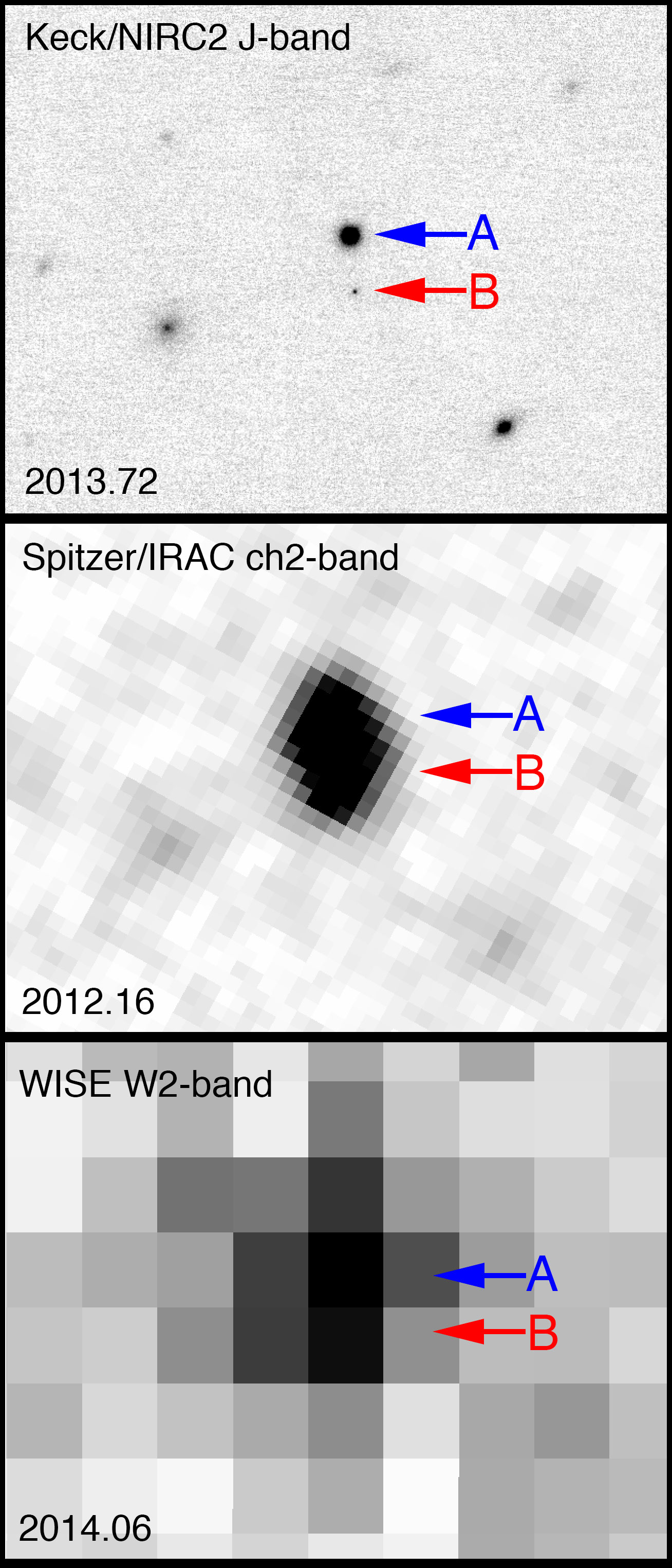
These four classes were considered for binary candidacy because a possible secondary could be affecting the flux measurements. This method has the potential to discover physical brown dwarf binaries with the components having the same distance, metallicity, and age. Figure 9 shows various imaging of WISE J022623.98021142.8 (Kirkpatrick et al. 2011), which is known to have a secondary component. We see that the binary is clearly separated in /NIRC2 (top panel; Gelino 2012), while in Spitzer/IRAC ch2 (middle panel; Kirkpatrick et al. 2021) and WISE/unTimely W2 (bottom panel; Meisner et al. 2022) it is blended. Note that the secondary is significantly redder in ch2 than the primary. Kirkpatrick et al. (2021) shows that for objects later than T5, the Jch2 color quickly changes towards very large values. Figure 14d of the same paper shows that the decrease of Mch2 with spectral type is less drastic. One can imagine a system like WISE J022623.98021142.8 for which the secondary is even colder. In this case, the ground-based band image might not have the sensitivity to detect the companion, but at the 4.6m wavelength of Spitzer, the presence of the companion could be detected. Thus, this technique has the potential to identify new binaries in which the companion objects are too low in temperature to be found in ground-based, band follow-up. Additionally, it also provides a priority target list of nearby brown dwarfs that may not yet have seen any high-resolution imaging follow-up. For example, if a late-T or early-Y dwarf has a secondary candidate around it, there is a possibility it would be the first ever mid-late Y dwarf found.
For Figure 6, which compares ch2PRF and W2PSF, we find that all the outliers were marked as Class 0. As illustrated in Figure 9, the poorer resolution of the WISE data blends the secondary more thoroughly with the primary, meaning that the WISE PSF fit is more successful at capturing the light of both components. In Figure 7, all but one outlier (mentioned in the caption) are identified as Class 1. This is because Class 1 objects are blended enough that a single PRF fit, though still poor, is not bad enough to trigger passive deblending, which would have made them Class 0 objects. Note that Classes 1-3 are numbered this way in order of the severity of the difference between the aperture and PRF-fit measurements. Class 0’s name results from its being a unique class compared to the rest.
6.2 Possible Contamination by Subdwarfs
The spectral energy distributions of subdwarfs show drastic differences compared to normal dwarfs within the wavelength ranges where they have been observed (Lodieu et al. 2019). Subdwarfs are the metal-poor counterparts to normal metallicity brown dwarfs (Lépine et al. 2003). This could affect how the point source looks on the detector. If there are large absorption bands in ch2/W2 that are drastically altering the effective wavelength through this bandpass, it would, because of the wavelength dependence of the MOPEX FWHM, change the full width half maximum value of the PRF. This difference between the expected PRF fit and the true PRF fit of a subdwarf would result in a high value. This is partly supported by the fact that one object in Class 3, 2MASS J064531536646120 (Kirkpatrick et al. 2010), is an L subdwarf. We have compared a “LOWZ”333https://doi.org/10.7910/DVN/SJRXUO (Meisner et al. 2021) spectral model of Z=1.5 and Teff=1300K to a solar-metallicity model at the same temperature. For the low-metallicity model, there is relatively more flux in the blue half of the W2 band compared to the solar-metallicity model. Based on this effect, we would expect a small change in the PRF width for the low-metallicity object, likely not large enough to support the hypothesis above. However, the models at these low-metallicities are completely untested in this wavelength regime. This effect can not be currently quantified because of the lack of observational spectra for subdwarfs at 4.6m. Further data, particularly from JWST (Gardner et al. 2006), will be needed to test this hypothesis. Nonetheless, as subdwarfs are rare in a volume-limited census, it is unlikely that this effect is the cause for any other aperture/PRF discrepancies within our sample.
6.3 Visual Inspection
To better understand Classes 0, 1, 2, and 3, we made finder charts for each object that include images from the Digitized Sky Survey 1 and 2 , , and ; the Pan-STARRS1 survey , , , , ; the UKIRT Infrared Deep Sky Survey , , and (Lawrence et al. 2007); the UKIRT Hemisphere Survey (Dye et al. 2018); the VISTA Hemisphere Survey and (McMahon et al. 2021); the Two Micron All Sky Survey , , and (Skrutskie et al. 2006); and WISE W1, W2, W3, and W4. These finder charts span a long time baseline and show the background sky at different epochs to see if our target was contaminated by a distant source at the Spitzer epochs. We also did a literature search for each object to check for binaries or subdwarfs. This led to the creation of 4 different subclasses: contaminated objects (C), potential binaries (P), known binaries (K), and subdwarfs (S).
6.4 Checking for true and false positives
Once the finder charts were made, it was then possible to search for an estimate of a true and false positive rate for the binary candidates. Although the finder charts provide a starting point for accessing false positives, high-resolution imaging is needed for more fully computing both the true and false positive rates.
To estimate a true positive rate, we searched two high-resolution archives and the literature for known binaries in classes 0 through 3. We searched papers in SIMBAD (Wenger et al., 2000) to find published binary systems. The two high-resolution archives we selected are the Keck Observatory Archive (hereafter, KOA; https://koa.ipac.caltech.edu) and the Hubble Space Telescope/NICMOS image archive studied in Factor & Kraus (2022). The known binary systems found, 12 in total, are listed in Table 5. Comparing this to our K+P+S lists of 72 objects we find an estimated true positive rate of 17. The true positive rate is likely higher because there are other high-resolution archives that could be searched, and there are some objects that have yet to be observed at high-resolution. This exercise is left for a future paper.
For some of our objects, a real false positive rate is impossible without high-resolution images at the same wavelengths as our Spitzer observations, 4.6m. Consider a binary T8 (the most abundant spectral type in our sample) and Y1 at a distance of 10pc. Using Figures 16(a) and 16(d) from Kirkpatrick et al. (2021), we find apparent J magnitudes of 18 mag for the T8 and 24 mag for the Y1, and apparent ch2 magnitudes of 13.5 mag for the T8 and 16 mag for the Y1. These values of J6 mag and J24 mag would make the secondary difficult/impossible to image, even with adaptive-optics imaging from the ground (Davies & Kasper 2012 and Zhang et al. 2021). However, values of ch22.5 mag and ch216 mag are much easier with Spitzer or JWST.
For earlier type primaries however, a false positive rate can be attempted because observations at 1m can provide a magnitude sufficient to rule out most secondaries detectable with our technique. Figure 4 of Gelino et al. (2011) shows the contrast ratios achievable for typical high-resolution observations for brown dwarf binary pairs. These ratios depend on the separation between the two objects, the primary’s brightness, and the dynamic range available for secondary detection. The contrast ratios start to plateau at binary separations of >. Since our ability to detect binaries is limited by the Spitzer/IRAC ch2 FWHM of , we can assume this plateau value. It is typical for ground based and NASA/ESA Hubble Space Telescope observations to have a depth of 22mag (Lowrance et al. 2005, Burgasser et al. 2006, and the Keck NIRC2 exposure time calculator444https://www2.keck.hawaii.edu/inst/nirc2/nirc2_snr_eff.html). A typical contrast ratio at wide separations is H4mag (Gelino et al., 2011). At our average distance of 15.9pc, an apparent magnitude of H=22mag would correspond to an absolute H magnitude of 21mag, or a spectral type of Y0 (Figure 16(b) of Kirkpatrick et al. 2021). A Y0 detection with H=4 mag is just achievable if the primary has a spectral type of T7.5. At primary spectral types earlier than this, a companion detectable via our Spitzer technique would likely also be detectable via ground based or Hubble Space Telescope observations.
In Table 4 the final column, labeled “High-Resolution Imaging”, indicates whether our candidate binary has high-resolution imaging observations in KOA or in Factor & Kraus (2022). There are 25 objects earlier than spectral type T7.5 with high-resolution imaging from these 2 archives. Using these data it is possible to estimate a false-positive rate. We will do this as follows. First, we compare our 25 false binaries to the total number of objects earlier than T7.5 in sub-classes K, P, and S (59) to provide a false positive rate of = 42. However, there are still 25 objects earlier than T7.5 not in Table 5 and lacking high-resolution imaging in Table 4, so this value is actually a (loose) lower bound for the false-positive rate. Second, we instead compare the same 25 false binaries to the subset of objects earlier than T7.5 with high-resolution imaging observations in Tables 4 and 5. This gives a new false-positive rate of = 74. However, this is likely an upper bound because the faintest companions to our 25 “false” binaries may not be detectable by our ground-based observations. In reality, we must wait for JWST 4.6m imaging to calculate a real false-positive rate, as an object lacking a companion detection at J-band might yet be harboring a cold companion seen only at longer wavelengths.
7 Discussion
7.1 Variability
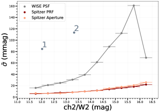
Figure 10 shows the median of the standard deviation as a function of ch2/W2 magnitude in 0.5-mag intervals. If an object has variability above the line, our analysis would have detected it. For example, if an object has a magnitude of 14.2, no variability can be detected below 12mmag (1) for the Spitzer photometry or 60mmag (1) for WISE photometry. Points 1 and 2 are known variable objects 2MASS J21392676+0220226 and 2MASS J222828894310262 (Yang et al. 2016), respectively (not included in this study). Number 1 and 2 can be seen to be well above all three lines, which indicates that variability could be found in the unTimely photometry and easily detected in our Spitzer photometry. Specifically, for 2MASS J21392676+0220226 we were able to find 14.5 variations in the unTimely W2 photometry, which is different from what is seen in Yang et al. (2016) which found Spitzer ch2 peak-to-peak variations of 26. Furthermore, this plot indicates that the unTimely data will only detect variability if it has relatively large amplitude, while the Spitzer data should be able to detect much smaller variations. If we instead looked at the magnitude percentage variations, we are sensitive to variability of >4 at 11.5 mag and >13 at 16 mag, for the unTimely photometry.
This study has shown no variability in brown dwarfs at 4.6m over a time period of >10 years to the sensitivity limits shown in Figure 10. The large-scale variability to which our survey is sensitive has only been seen in a small number of published objects. This illustrates that large-amplitude variability is rare among brown dwarfs. At smaller amplitudes, however, Yang et al. (2016)) found an increase in the percentage of objects with variability near the L/T transition compared to those in the T/Y transition. Figure 2 shows that we have excellent statistics at the T/Y transition, yet we find no large-amplitude variability there.
7.2 Binarity
Brown dwarf binaries are rare and hard to find. Two common ways to find brown dwarf binaries are obtaining a spectrum of a clear spectral composite object (Bardalez Gagliuffi et al. 2014) or visually separating the components via imaging. Our Aperture-PRF technique provides a new way of finding these binaries, in much the same way that the PRF technique alone, through passive deblending, has previously been used to find secondary components (e.g., in circumstellar disks; Martinez & Kraus 2019).
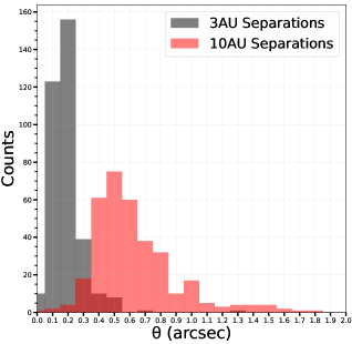
We now compare the MOPEX FWHM of Spitzer to the average separation of known nearby brown dwarf binaries, to test our binary hypothesis. The MOPEX FWHM of Spitzer is at ch2 (4.6m). Figure 2 of Burgasser et al. (2007) shows that the average brown dwarf binary has a physical separation between 3 10 AU. When considering the average distance for our 361 objects is 15.9pc, this leads to an expected separation between . The distribution of the 361 objects angular separation based on distance assuming 3 and 10AU binary separation can be seen in Figure 11. We see that the objects clump around the predicted separations. However, there are a few objects that are outside of this separation, indicating that they could be angularly separated in the Spitzer photometry. Objects of Class 0 must have separation > in order for the code to passively deblend the object into two different PRF fits. This separation means that Class 0 is very unlikely to have physical binaries. Objects of Class 1, 2, and 3 are only marginally resolved or are within the MOPEX FWHM, meaning that Class 1-3 are the ones most likely to have hidden, faint secondaries.
| C | K | P | S | Total | |
|---|---|---|---|---|---|
| Class 0 | 10 | 1 | 5 | 0 | 16 |
| Class 1 | 3 | 3 | 5 | 0 | 11 |
| Class 2 | 18 | 3 | 14 | 0 | 35 |
| Class 3 | 23 | 5 | 35 | 1 | 64 |
| Total | 54 | 12 | 59 | 1 | 126 |
Reference Codes: (C) Contaminated objects, (K) Known binaries, (P) Potential binaries, and (S) Subdwarfs
In Table LABEL:table_2 we show how many objects fall in each class and subclass as defined in §6.1 and §6.3. Details of all 126 objects can be found in Tables 3, 4, and 5. There was only one subdwarf found in this process, 2MASS J064531536646120, listed in Table 5 with the known binaries.
We compare known binary/contaminated statistics below for each class:
-
•
Class 0: Only 1 known binary was found. Most known brown dwarf binaries have separation smaller than the separations at which passive deblending ( to ) would take place. Contamination by background objects is the highest among all four classes ( = 63).
-
•
Class 1: This is the highest percentage of known binaries of all four groups ( = 27). The true binaries in this class are likely to have the smallest mag and/or largest separations, because they have the most discrepant aperture and PRF-fit measurements. Class 1 also has a significant percentage of background contamination ( = 27).
-
•
Class 2: This class has a much smaller percentage of known binaries ( = 9). True binaries here will likely have slightly larger mag and smaller separations. Contamination by background objects is high ( = 51).
-
•
Class 3: This class has the smallest percentage of known binaries ( = 8) and sizable percentage of background contamination ( = 36). Given the smaller difference between aperture and PRF-fit measures, this group is likely to have more spurious binaries than the other classes, but could also have binaries with the tightest separation and/or largest mags.
8 Conclusion
We examined two 4.6m photometric datasets, Spitzer/IRAC ch2 and unTimely W2, to analyze long-term variability in brown dwarfs. Using the Spitzer/IRAC ch2 photometry, our study establishes that the typical ch2 variability on 10 year time scales is <8mmag for objects at ch2 = 11.5 mag and <22mmag for objects at ch2 = 16 mag. Using the unTimely photometry, which has higher uncertainties than Spitzer/IRAC ch2, we find that all variations must be <4.5 at 11.5 mag and <12.5 at 16 mag. Although a handful of objects in the literature have been reported with variations greater than this, we conclude that higher-amplitude variability must be the exception rather than the rule.
We also demonstrate a new technique for the identification of brown dwarf binary candidates that uses a comparison of Spitzer’s aperture and PRF-fit photometry. We present a table of 59 previously unrecognized candidate binaries (Table 4) that constitute prime targets for high-resolution follow-up imaging.
9 Acknowledgement
This Backyard Worlds research was supported by NASA grant 2017-ADAP17-0067. We thank the Student Astrophysics Society555https://www.studentastrophysicssociety.com for providing the resources that enabled the pairing of high school and undergraduate students with practicing astronomers. This work makes use of data products from WISE/NEOWISE, which is a joint project of UCLA and JPL/Caltech, funding by NASA.
Work in this paper is based on observations made with the Spitzer Space Telescope, which is operated by JPL/Caltech, under a contract with NASA. Support for the original parallax work was provided to J.D.K. by NASA through a Cycle 14 award issued by JPL/Caltech. Some data presented here were obtained at the W. M. Keck Observatory, which is operated as a scientific partnership among Caltech, the University of California, and NASA. The authors wish to recognize and acknowledge the very significant cultural role and reverence that the summit of Maunakea has always had within the indigenous Hawaiian community. We are most fortunate to have the opportunity to conduct observations from this mountain. The Observatory was made possible by the generous financial support of the W. M. Keck Foundation. This research has made use of the Keck Observatory Archive (KOA), which is operated by the W. M. Keck Observatory and the NASA Exoplanet Science Institute (NExScI), under contract with the National Aeronautics and Space Administration. This research has made use of the NASA/IPAC Infrared Science Archive, which is funded by the National Aeronautics and Space Administration and operated by the California Institute of Technology. This research has made use of the SIMBAD database, operated at CDS, Strasbourg, France
The Digitized Sky Survey was produced at the Space Telescope Science Institute under U.S. Government grant NAG W-2166. The images of these surveys are based on photographic data obtained using the Oschin Schmidt Telescope on Palomar Mountain and the UK Schmidt Telescope. The plates were processed into the present compressed digital form with the permission of these institutions. Our finder charts also used observations obtained as part of the VISTA Hemisphere Survey, ESO Progam, 179.A-2010 (PI: McMahon). The UHS is a partnership between the UK STFC, The University of Hawaii, The University of Arizona, Lockheed Martin and NASA.
The Pan-STARRS1 Surveys (PS1) and the PS1 public science archive have been made possible through contributions by the Institute for Astronomy, the University of Hawaii, the Pan-STARRS Project Office, the Max-Planck Society and its participating institutes, the Max Planck Institute for Astronomy, Heidelberg and the Max Planck Institute for Extraterrestrial Physics, Garching, The Johns Hopkins University, Durham University, the University of Edinburgh, the Queen’s University Belfast, the Harvard-Smithsonian Center for Astrophysics, the Las Cumbres Observatory Global Telescope Network Incorporated, the National Central University of Taiwan, the Space Telescope Science Institute, the National Aeronautics and Space Administration under Grant No. NNX08AR22G issued through the Planetary Science Division of the NASA Science Mission Directorate, the National Science Foundation Grant No. AST-1238877, the University of Maryland, Eotvos Lorand University (ELTE), the Los Alamos National Laboratory, and the Gordon and Betty Moore Foundation.
References
- Allers et al. (2007) Allers, K. N., Jaffe, D. T., Luhman, K. L., et al. 2007, ApJ, 657, 511. doi:10.1086/510845
- Apai et al. (2017) Apai, D., Karalidi, T., Marley, M. S., et al. 2017, Science, 357, 683. doi:10.1126/science.aam9848
- Artigau et al. (2009) Artigau, É., Bouchard, S., Doyon, R., et al. 2009, ApJ, 701, 1534. doi:10.1088/0004-637X/701/2/1534
- Artigau et al. (2011) Artigau, É., Lafrenière, D., Doyon, R., et al. 2011, ApJ, 739, 48. doi:10.1088/0004-637X/739/1/48
- Artigau (2018) Artigau, É. 2018, Handbook of Exoplanets, 94. doi:10.1007/978-3-319-55333-7_94
- Bailer-Jones & Mundt (1999) Bailer-Jones, C. A. L. & Mundt, R. 1999, A&A, 348, 800
- Bardalez Gagliuffi et al. (2014) Bardalez Gagliuffi, D. C., Burgasser, A. J., Gelino, C. R., et al. 2014, ApJ, 794, 143.doi:10.1088/0004-637X/794/2/143
- Bardalez Gagliuffi et al. (2015) Bardalez Gagliuffi, D. C., Gelino, C. R., & Burgasser, A. J. 2015, AJ, 150, 163. doi:10.1088/0004-6256/150/5/163
- Bardalez Gagliuffi et al. (2019) Bardalez Gagliuffi, D., Ward-Duong, K., Faherty, J., et al. 2019, BAAS, 51, 285
- Beichman et al. (2013) Beichman, C., Gelino, C. R., Kirkpatrick, J. D., et al. 2013, ApJ, 764, 101. doi:10.1088/0004-637X/764/1/101
- Best et al. (2021) Best, W. M. J., Liu, M. C., Magnier, E. A., et al. 2021, AJ, 161, 42. doi:10.3847/1538-3881/abc893
- Burgasser et al. (2006) Burgasser, A. J., Kirkpatrick, J. D., Cruz, K. L., et al. 2006, ApJS, 166, 585. doi:10.1086/506327
- Burgasser et al. (2007) Burgasser, A. J., Reid, I. N., Siegler, N., et al. 2007, Protostars and Planets V, 427
- Burgasser et al. (2010) Burgasser, A. J., Cruz, K. L., Cushing, M., et al. 2010, ApJ, 710, 1142. doi:10.1088/0004-637X/710/2/1142
- Cushing et al. (2016) Cushing, M. C., Hardegree-Ullman, K. K., Trucks, J. L., et al. 2016, ApJ, 823, 152. doi:10.3847/0004-637X/823/2/152
- Davies & Kasper (2012) Davies, R. & Kasper, M. 2012, ARA&A, 50, 305. doi:10.1146/annurev-astro-081811-125447
- Deacon et al. (2017) Deacon, N. R., Magnier, E. A., Best, W. M. J., et al. 2017, MNRAS, 468, 3499. doi:10.1093/mnras/stx440
- Deming et al. (2015) Deming, D., Knutson, H., Kammer, J., et al. 2015, ApJ, 805, 132. doi:10.1088/0004-637X/805/2/132
- Ducrot et al. (2020) Ducrot, E., Gillon, M., Delrez, L., et al. 2020, A&A, 640, A112. doi:10.1051/0004-6361/201937392
- Dye et al. (2018) Dye, S., Lawrence, A., Read, M. A., et al. 2018, MNRAS, 473, 5113. doi:10.1093/mnras/stx2622
- Eriksson et al. (2019) Eriksson, S. C., Janson, M., & Calissendorff, P. 2019, A&A, 629, A145. doi:10.1051/0004-6361/201935671
- Esplin et al. (2016) Esplin, T. L., Luhman, K. L., Cushing, M. C., et al. 2016, ApJ, 832, 58. doi:10.3847/0004-637X/832/1/58
- Factor & Kraus (2022) Factor, S. M. & Kraus, A. L. 2022, AJ, 164, 244. doi:10.3847/1538-3881/ac88d3
- Fazio et al. (2004) Fazio, G. G., Hora, J. L., Allen, L. E., et al. 2004, ApJS, 154, 10. doi:10.1086/422843
- Gardner et al. (2006) Gardner, J. P., Mather, J. C., Clampin, M., et al. 2006, Space Sci. Rev., 123, 485. doi:10.1007/s11214-006-8315-710.48550/arXiv.astro-ph/0606175
- Ge et al. (2019) Ge, H., Zhang, X., Fletcher, L. N., et al. 2019, AJ, 157, 89. doi:10.3847/1538-3881/aafba7
- Gelino & Marley (2000) Gelino, C. & Marley, M. 2000, From Giant Planets to Cool Stars, 212, 322
- Gelino et al. (2011) Gelino, C. R., Kirkpatrick, J. D., Cushing, M. C., et al. 2011, AJ, 142, 57. doi:10.1088/0004-6256/142/2/57
- Gelino (2012) Gelino, C. 2012, Keck Observatory Archive NIRC2, N099N2L
- Gizis et al. (2017) Gizis, J. E., Paudel, R. R., Mullan, D., et al. 2017, ApJ, 845, 33. doi:10.3847/1538-4357/aa7da0
- Hirst & Cardenes (2016) Hirst, P. & Cardenes, R. 2016, Proc. SPIE, 9913, 99131E. doi:10.1117/12.2231833
- Hora et al. (2012) Hora, J. L., Marengo, M., Park, R., et al. 2012, Proc. SPIE, 8442, 844239. doi:10.1117/12.926894
- IRSA (2022) IRSA, 2022, Spitzer Heritage Archive, IPAC, doi:10.26131/IRSA543
- Kellogg et al. (2017) Kellogg, K., Metchev, S., Heinze, A., et al. 2017, ApJ, 849, 72. doi:10.3847/1538-4357/aa8e4f
- Kendall et al. (2007) Kendall, T. R., Jones, H. R. A., Pinfield, D. J., et al. 2007, MNRAS, 374, 445. doi:10.1111/j.1365-2966.2006.11026.x
- Kirkpatrick et al. (2010) Kirkpatrick, J. D., Looper, D. L., Burgasser, A. J., et al. 2010, ApJS, 190, 100. doi:10.1088/0067-0049/190/1/100
- Kirkpatrick et al. (2011) Kirkpatrick, J. D., Cushing, M. C., Gelino, C. R., et al. 2011, ApJS, 197, 19. doi:10.1088/0067-0049/197/2/19
- Kirkpatrick et al. (2016) Kirkpatrick, J. D., Schneider, A., Fajardo-Acosta, S., et al. 2016, VizieR Online Data Catalog, J/ApJ/783/122
- Kirkpatrick et al. (2019) Kirkpatrick, J. D., Martin, E. C., Smart, R. L., et al. 2019, ApJS, 240, 19. doi:10.3847/1538-4365/aaf6af
- Kirkpatrick et al. (2021) Kirkpatrick, J. D., Gelino, C. R., Faherty, J. K., et al. 2021, ApJS, 253, 7. doi:10.3847/1538-4365/abd107
- Kolb & Baraffe (1999) Kolb, U. & Baraffe, I. 1999, MNRAS, 309, 1034. doi:10.1046/j.1365-8711.1999.02926.x
- Lang (2014) Lang, D. 2014, AJ, 147, 108. doi:10.1088/0004-6256/147/5/108
- Lawrence et al. (2007) Lawrence, A., Warren, S. J., Almaini, O., et al. 2007, MNRAS, 379, 1599. doi:10.1111/j.1365-2966.2007.12040.x
- Lee et al. (2018) Lee, E. K. H., Blecic, J., & Helling, C. 2018, A&A, 614, A126. doi:10.1051/0004-6361/201731977
- Leggett et al. (2016) Leggett, S. K., Cushing, M. C., Hardegree-Ullman, K. K., et al. 2016, ApJ, 830, 141. doi:10.3847/0004-637X/830/2/141
- Lépine et al. (2003) Lépine, S., Rich, R. M., & Shara, M. M. 2003, ApJ, 591, L49. doi:10.1086/377069
- Limbach et al. (2021) Limbach, M. A., Vos, J. M., Winn, J. N., et al. 2021, ApJ, 918, L25. doi:10.3847/2041-8213/ac1e2d
- Liu et al. (2012) Liu, M. C., Dupuy, T. J., Bowler, B. P., et al. 2012, ApJ, 758, 57. doi:10.1088/0004-637X/758/1/57
- Lodieu et al. (2019) Lodieu, N., Allard, F., Rodrigo, C., et al. 2019, A&A, 628, A61. doi:10.1051/0004-6361/201935299
- Lowrance et al. (2005) Lowrance, P. J., Becklin, E. E., Schneider, G., et al. 2005, AJ, 130, 1845. doi:10.1086/432839
- Luhman (2012) Luhman, K. L. 2012, ARA&A, 50, 65. doi:10.1146/annurev-astro-081811-125528
- Mace (2014) Mace, G. N. 2014, VizieR Online Data Catalog, V/144
- Mainzer et al. (2011) Mainzer, A., Bauer, J., Grav, T., et al. 2011, ApJ, 731, 53. doi:10.1088/0004-637X/731/1/53
- Mainzer et al. (2014) Mainzer, A., Bauer, J., Cutri, R. M., et al. 2014, ApJ, 792, 30. doi:10.1088/0004-637X/792/1/30
- Makovoz & Marleau (2005) Makovoz, D. & Marleau, F. R. 2005, PASP, 117, 1113. doi:10.1086/432977
- Makovoz et al. (2006) Makovoz, D., Roby, T., Khan, I., et al. 2006, Proc. SPIE, 6274, 62740C. doi:10.1117/12.672536
- Marley et al. (2013) Marley, M. S., Ackerman, A. S., Cuzzi, J. N., et al. 2013, Comparative Climatology of Terrestrial Planets, 367. doi:10.2458/azu_uapress_9780816530595-ch015
- Martinez & Kraus (2019) Martinez, R. A. & Kraus, A. L. 2019, AJ, 158, 134. doi:10.3847/1538-3881/ab32e6
- Mason et al. (2001) Mason, B. D., Wycoff, G. L., Hartkopf, W. I., et al. 2001, AJ, 122, 3466. doi:10.1086/323920
- McMahon et al. (2021) McMahon, R. G., Banerji, M., Gonzalez, E., et al. 2021, VizieR Online Data Catalog, II/367
- Schlafly, Meisner, & Green (2019) Meisner, A. & Schlafly, E. 2019, Astrophysics Source Code Library. ascl:1901.004
- Meisner et al. (2020) Meisner, A. M., Faherty, J. K., Kirkpatrick, J. D., et al. 2020, ApJ, 899, 123. doi:10.3847/1538-4357/aba633
- Meisner et al. (2021) Meisner, A. M., Schneider, A. C., Burgasser, A. J., et al. 2021, ApJ, 915, 120. doi:10.3847/1538-4357/ac013c10.48550/arXiv.2106.01387
- Meisner et al. (2022) Meisner, A. M., Lang, D., Schlafly, E. F., et al. 2022, arXiv:2204.05748
- Metchev et al. (2015) Metchev, S. A., Heinze, A., Apai, D., et al. 2015, ApJ, 799, 154. doi:10.1088/0004-637X/799/2/154
- Moore et al. (2019) Moore, K., Scholz, A., & Jayawardhana, R. 2019, ApJ, 872, 159. doi:10.3847/1538-4357/aaff5c
- Müller et al. (2016) Müller, T. G., Balog, Z., Nielbock, M., et al. 2016, A&A, 588, A109. doi:10.1051/0004-6361/201527371
- Nelson et al. (1986) Nelson, L. A., Rappaport, S. A., & Joss, P. C. 1986, ApJ, 311, 226. doi:10.1086/164767
- Radigan et al. (2012) Radigan, J., Jayawardhana, R., Lafrenière, D., et al. 2012, ApJ, 750, 105. doi:10.1088/0004-637X/750/2/105
- Radigan et al. (2014a) Radigan, J., Lafrenière, D., Jayawardhana, R., et al. 2014a, ApJ, 793, 75. doi:10.1088/0004-637X/793/2/75
- Radigan (2014b) Radigan, J. 2014b, ApJ, 797, 120. doi:10.1088/0004-637X/797/2/120
- Reach et al. (2005) Reach, W. T., Megeath, S. T., Cohen, M., et al. 2005, PASP, 117, 978. doi:10.1086/432670
- Reid et al. (2006) Reid, I. N., Lewitus, E., Allen, P. R., et al. 2006, AJ, 132, 891. doi:10.1086/505626
- Reid et al. (2008) Reid, I. N., Cruz, K. L., Burgasser, A. J., et al. 2008, AJ, 135, 580. doi:10.1088/0004-6256/135/2/580
- Rowe-Gurney et al. (2021) Rowe-Gurney, N., Fletcher, L. N., Orton, G. S., et al. 2021, Icarus, 365, 114506. doi:10.1016/j.icarus.2021.114506
- Schlafly et al. (2012) Schlafly, E. F., Finkbeiner, D. P., Jurić, M., et al. 2012, ApJ, 756, 158. doi:10.1088/0004-637X/756/2/158
- Schlafly et al. (2019) Schlafly, E. F., Meisner, A. M., & Green, G. M. 2019, ApJS, 240, 30. doi:10.3847/1538-4365/aafbea
- Simon et al. (2021) Simon, A., Orton, G. S., & Wong, M. H. 2021, HST Proposal, 16790
- Skrutskie et al. (2006) Skrutskie, M. F., Cutri, R. M., Stiening, R., et al. 2006, AJ, 131, 1163. doi:10.1086/498708
- Softich et al. (2022) Softich, E., Schneider, A. C., Patience, J., et al. 2022, ApJ, 926, L12. doi:10.3847/2041-8213/ac51d8
- Stauffer et al. (2016) Stauffer, J., Marley, M. S., Gizis, J. E., et al. 2016, AJ, 152, 142. doi:10.3847/0004-6256/152/5/142
- Tamburo et al. (2022) Tamburo, P., Muirhead, P. S., McCarthy, A. M., et al. 2022, AJ, 163, 253. doi:10.3847/1538-3881/ac64aa
- Tannock et al. (2021) Tannock, M. E., Metchev, S., Heinze, A., et al. 2021, AJ, 161, 224. doi:10.3847/1538-3881/abeb67
- Tran et al. (2004) Tran, H. D., Mader, J., Conrad, A., et al. 2004, \aas
- Tsuji (2005) Tsuji, T. 2005, ApJ, 621, 1033. doi:10.1086/427747
- Vos et al. (2022) Vos, J. M., Faherty, J. K., Gagné, J., et al. 2022, ApJ, 924, 68. doi:10.3847/1538-4357/ac4502
- Wenger et al. (2000) Wenger, M., Ochsenbein, F., Egret, D., et al. 2000, A&AS, 143, 9. doi:10.1051/aas:2000332
- Werner et al. (2004) Werner, M. W., Roellig, T. L., Low, F. J., et al. 2004, ApJS, 154, 1. doi:10.1086/422992
- Wright et al. (2010) Wright, E. L., Eisenhardt, P. R. M., Mainzer, A. K., et al. 2010, AJ, 140, 1868. doi:10.1088/0004-6256/140/6/1868
- Yang et al. (2016) Yang, H., Apai, D., Marley, M. S., et al. 2016, ApJ, 826, 8. doi:10.3847/0004-637X/826/1/8
- Zhang et al. (2017) Zhang, Z. H., Pinfield, D. J., Gálvez-Ortiz, M. C., et al. 2017, MNRAS, 464, 3040. doi:10.1093/mnras/stw2438
- Zhang et al. (2021) Zhang, J., Cooke, J., Canalizo, G., et al. 2021, GRB Coordinates Network, Circular Service, No. 30858, 30858
| Object Name | RA (deg) | Dec (deg) | Class | Subclass |
|---|---|---|---|---|
| WISE J004945.61+215120.0 | 12.439581 | 21.855476 | 3 | C |
| 2MASSW J0051107154417 | 12.79513 | 15.73814 | 2 | C |
| WISEA J005811.69565332.1 | 14.54965 | 56.892303 | 3 | C |
| 2MASSI J0103320+193536 | 15.88506 | 19.593263 | 3 | C |
| CWISEP J010527.69783419.3 | 16.370636 | 78.572554 | 0 | C |
| CWISE J014837.51104805.6 | 27.15694 | 10.801799 | 2 | C |
| WISEPA J031325.96+780744.2 | 48.359129 | 78.129099 | 2 | C |
| WISE J032301.86+562558.0 | 50.75963 | 56.431894 | 3 | C |
| WISEPC J033349.34585618.7 | 53.457085 | 58.939765 | 3 | C |
| WISE J033515.01+431045.1 | 53.813599 | 43.177629 | 3 | C |
| 2MASS J034009426724051 | 55.034396 | 67.398518 | 1 | C |
| 2MASS J035822554116060 | 59.594508 | 41.267803 | 2 | C |
| 2MASS J042107186306022 | 65.281665 | 63.099437 | 2 | C |
| 2MASSI J0443058320209 | 70.77379 | 32.034919 | 0 | C |
| PSO J076.7092+52.6087 | 76.709485 | 52.608231 | 0 | C |
| 2MASSI J0512063294954 | 78.026636 | 29.831269 | 2 | C |
| WISE J052126.29+102528.4 | 80.360194 | 10.423512 | 0 | C |
| CWISEP J063428.10+504925.9 | 98.618859 | 50.822681 | 2 | C |
| WISE J064205.58+410155.5 | 100.52362 | 41.031459 | 3 | C |
| 2MASS J074142790506464 | 115.42829 | 5.11289 | 0 | C |
| ULAS J074502.79+233240.3 | 116.26163 | 23.54453 | 0 | C |
| WISE J105130.01213859.7 | 162.87537 | 21.650142 | 2 | C |
| SIMP J113220583809562 | 173.08717 | 38.166428 | 3 | C |
| WISE J125715.90+400854.2 | 194.31615 | 40.14811 | 2 | C |
| 2MASS J14075361+1241099 | 211.97158 | 12.686486 | 3 | C |
| CWISEP J145837.91+173450.1 | 224.65736 | 17.580799 | 0 | C |
| 2MASSI J1526140+204341 | 231.55718 | 20.726056 | 2 | C |
| CWISEP J153859.39+482659.1 | 234.74805 | 48.44905 | 3 | C |
| WISEA J162341.27740230.4 | 245.92 | 74.04263 | 2 | C |
| WISE J163940.86684744.6 | 249.92274 | 68.798677 | 3 | C |
| PSO J258.2413+06.7612 | 258.24107 | 6.761227 | 1 | C |
| WISEA J173453.90481357.9 | 263.72383 | 48.233351 | 2 | C |
| WISEA J173551.56820900.3 | 263.96544 | 82.150738 | 3 | C |
| WISE J174102.78464225.5 | 265.26168 | 46.707965 | 2 | C |
| WISE J175510.28+180320.2 | 268.79212 | 18.056078 | 3 | C |
| WISE J180952.53044812.5 | 272.46884 | 4.804453 | 1 | C |
| WISEA J181849.59470146.9 | 274.70665 | 47.030892 | 0 | C |
| CWISE J183207.94540943.3 | 278.03261 | 54.162757 | 3 | C |
| WISE J185101.83+593508.6 | 282.75777 | 59.586189 | 3 | C |
| WISE J191915.54+304558.4 | 289.81597 | 30.767298 | 3 | C |
| 2MASS J19251275+0700362 | 291.30355 | 7.011064 | 0 | C |
| WISENF J193656.08+040801.2 | 294.2323 | 4.131147 | 2 | C |
| WISE J200050.19+362950.1 | 300.20898 | 36.497832 | 3 | C |
| WISE J201404.13+042408.5 | 303.51622 | 4.40277 | 2 | C |
| WISEA J201833.67141720.3 | 304.64037 | 14.288602 | 3 | C |
| 2MASS J21265916+7617440 | 321.76234 | 76.29985 | 2 | C |
| 2MASS J21543318+5942187 | 328.637 | 59.70326 | 3 | C |
| WISE J223617.59+510551.9 | 339.07618 | 51.098434 | 3 | C |
| WISEP J223937.55+161716.2 | 339.90682 | 16.288033 | 3 | C |
| 2MASS J22490917+3205489 | 342.29281 | 32.095967 | 2 | C |
| WISEA J230228.66713441.7 | 345.61789 | 71.579123 | 3 | C |
| 2MASS J23254530+4251488 | 351.43842 | 42.861899 | 0 | C |
| 2MASS J233123784718274 | 352.84951 | 47.30787 | 3 | C |
| 2MASSI J2339101+135230 | 354.79477 | 13.869448 | 2 | C |
| Object Name | RA (deg) | Dec (deg) | Class | Subclass | High-Resolution ImagingbbKeck: High-resolution imaging from the Keck Observatory Archive (https://koa.ipac.caltech.edu), HST: High-resolution imaging from the HST/NICMOS image archive studied in Factor & Kraus (2022) |
|---|---|---|---|---|---|
| WISE J000517.48+373720.5ccObject with spectral type T7.5 or later | 1.3243156 | 37.622133 | 3 | P | Keck |
| 2MASS J00345157+0523050 | 8.7173945 | 5.385477 | 3 | P | Keck |
| WISE J011154.36505343.2 | 17.975789 | 50.895856 | 3 | P | |
| 2MASS J01550354+0950003 | 28.76651 | 9.832968 | 0 | P | HST |
| WISEA J020047.29510521.4 | 30.197571 | 51.089537 | 3 | P | |
| 2MASSW J0205034+125142 | 31.26636 | 12.86154 | 2 | P | |
| WISEA J030237.53581740.3ccObject with spectral type T7.5 or later | 45.656221 | 58.294742 | 3 | P | |
| WISEA J030919.70501614.2 | 47.333383 | 50.270291 | 3 | P | |
| 2MASS J031014012756452 | 47.55754 | 27.946302 | 2 | P | Keck |
| 2MASS J031854033421292 | 49.727839 | 34.357738 | 1 | P | HST |
| SDSSp J033035.13002534.5 | 52.64629 | 0.42628 | 3 | P | |
| PSO J052.721403.8409 | 52.72142 | 3.84092 | 3 | P | Keck |
| WISE J033651.90+282628.8 | 54.216403 | 28.44105 | 3 | P | |
| 2MASSW J0337036175807 | 54.26496 | 17.96886 | 2 | P | Keck |
| WISE J045746.08020719.2 | 74.442276 | 2.122342 | 3 | P | Keck |
| 2MASS J06020638+4043588 | 90.528129 | 40.732372 | 3 | P | Keck |
| 2MASS J075554303259589 | 118.97545 | 32.998815 | 3 | P | |
| SDSS J075840.33+324723.4 | 119.66821 | 32.79014 | 3 | P | |
| WISEPC J075946.98490454.0ccObject with spectral type T7.5 or later | 119.94553 | 49.081232 | 3 | P | |
| WISEA J082640.45164031.8 | 126.66664 | 16.674235 | 3 | P | Keck |
| WISEPC J083641.12185947.2ccObject with spectral type T7.5 or later | 129.17153 | 18.996518 | 2 | P | Keck |
| SDSS J085234.90+472035.0 | 133.14493 | 47.34106 | 2 | P | Keck |
| WISEPA J085716.25+560407.6ccObject with spectral type T7.5 or later | 134.31581 | 56.068336 | 3 | P | Keck |
| SDSSp J085758.45+570851.4 | 134.4911 | 57.1464 | 3 | P | |
| 2MASS J09054654+5623117 | 136.44392 | 56.38661 | 0 | P | Keck |
| WISE J092055.40+453856.3 | 140.23088 | 45.64886 | 3 | P | |
| 2MASSI J1010148040649 | 152.56001 | 4.113933 | 3 | P | |
| 2MASSW J1036530344138 | 159.22075 | 34.696486 | 2 | P | |
| WISE J103907.73160002.9ccObject with spectral type T7.5 or later | 159.78173 | 16.001139 | 3 | P | Keck |
| 2MASS J10430758+2225236 | 160.7809 | 22.423186 | 2 | P | HST |
| 2MASSI J1104012+195921 | 166.00555 | 19.989852 | 1 | P | HST |
| CFBDS J111807064016 | 169.52805 | 6.669126 | 0 | P | Keck |
| WISEP J115013.88+630240.7ccObject with spectral type T7.5 or later | 177.56027 | 63.044022 | 3 | P | Keck |
| SDSS J115553.86+055957.5 | 178.97306 | 5.999081 | 3 | P | Keck |
| SDSSp J120358.19+001550.3 | 180.98575 | 0.26256 | 1 | P | |
| 2MASSI J1213033043243 | 183.26275 | 4.545563 | 3 | P | HST |
| SDSS J121951.45+312849.4 | 184.96319 | 31.480466 | 3 | P | |
| 2MASS J123147.53+084733.1 | 187.94283 | 8.788455 | 3 | P | |
| PSO J201.0320+19.1072 | 201.03179 | 19.106953 | 2 | P | |
| 2MASS J13243559+6358284aaPossible spectral binary (Burgasser et al., 2010) | 201.14508 | 63.974268 | 3 | P | |
| SDSSp J132629.82003831.5 | 201.62282 | 0.642752 | 3 | P | |
| WISE J140035.40385013.5 | 210.14758 | 38.83746 | 3 | P | Keck |
| SDSS J153453.33+121949.2 | 233.72292 | 12.330219 | 0 | P | |
| PSO J247.3273+03.5932 | 247.32757 | 3.592974 | 3 | P | Keck |
| WISE J165842.56+510335.0 | 254.67684 | 51.059217 | 3 | P | Keck |
| WISE J172134.46+111739.4 | 260.39341 | 11.294473 | 2 | P | Keck |
| WISEA J172907.10753017.0ccObject with spectral type T7.5 or later | 262.27553 | 75.505234 | 3 | P | |
| 2MASS J17461199+5034036 | 266.55258 | 50.567694 | 2 | P | |
| WISE J181329.40+283533.3ccObject with spectral type T7.5 or later | 273.37128 | 28.591289 | 3 | P | Keck |
| 2MASS J19010601+4718136 | 285.27586 | 47.305732 | 3 | P | Keck |
| WISE J203042.79+074934.7 | 307.68001 | 7.826027 | 2 | P | Keck |
| WISE J204356.42+622048.9 | 310.98754 | 62.347831 | 1 | P | Keck |
| PSO J319.310229.6682 | 319.31057 | 29.668531 | 3 | P | Keck |
| CWISEP J213249.05+690113.7ccObject with spectral type T7.5 or later | 323.20562 | 69.020736 | 2 | P | |
| 2MASS J21373742+0808463 | 324.40963 | 8.146552 | 1 | P | Keck |
| WISE J214155.85511853.1 | 325.48432 | 51.31501 | 2 | P | |
| 2MASS J231747124838501 | 349.4483 | 48.646791 | 2 | P | |
| WISEPC J232728.75273056.5 | 351.86997 | 27.515783 | 3 | P | |
| 2MASS J234406240733282 | 356.02605 | 7.5584 | 0 | P |
| Object Name | RA (deg) | Dec (deg) | Class | Subclass | Ref |
|---|---|---|---|---|---|
| WISE J003110.04+574936.3 | 7.79433 | 57.826773 | 2 | K | 1 |
| WISEPC J013836.59032221.2 | 24.652471 | 3.373118 | 3 | K | 2 |
| WISEPA J022623.98021142.8 | 36.599284 | 2.195299 | 1 | K | 3 |
| WISEPA J045853.89+643452.9aaObject with spectral type T7.5 or later | 74.725621 | 64.5818 | 3 | K | 4 |
| WISEA J064750.85154616.4 | 101.96192 | 15.77122 | 0 | K | 1 |
| PSO J103.0927+41.4601 | 103.09287 | 41.460042 | 2 | K | 1 |
| WISEPC J121756.91+162640.2aaObject with spectral type T7.5 or later | 184.48809 | 16.443144 | 1 | K | 5 |
| SIMP J1619275+031350 | 244.86502 | 3.229445 | 1 | K | 6 |
| WISEPA J171104.60+350036.8aaObject with spectral type T7.5 or later | 257.76888 | 35.010238 | 2 | K | 5 |
| 2MASS J21522609+0937575 | 328.10965 | 9.633177 | 3 | K | 7 |
| PSO J330.3214+32.3686 | 330.32183 | 32.368747 | 3 | K | 2 |
| 2MASS J225518615713056 | 343.82535 | 57.2197 | 3 | K | 8 |
| 2MASS J064531536646120 | 101.36693 | 66.76297 | 3 | S | 9 |
Note. — Reference Codes: (1) Best et al. (2021), (2) Unpublished data in the Keck Observatory Archive (https://koa.ipac.caltech.edu), (3) Kirkpatrick et al. (2019), (4) Gelino et al. (2011), (5) Liu et al. (2012), (6) Artigau et al. (2011), (7) Reid et al. (2006), (8) Reid et al. (2008), (9) Kirkpatrick et al. (2010)