This paper was converted on www.awesomepapers.org from LaTeX by an anonymous user.
Want to know more? Visit the Converter page.

Long time dynamics of a three-species food chain model with Allee effect in the top predator

Abstract

The Allee effect is an important phenomenon in population biology characterized by positive density dependence, that is a positive correlation between population density and individual fitness. However, the effect is not well studied in multi-level trophic food chains. We consider a ratio dependent spatially explicit three species food chain model, where the top predator is subjected to a strong Allee effect. We show the existence of a global attractor for the the model, that is upper semicontinuous in the Allee threshold parameter mm. To the best of our knowledge this is the first robustness result, for a spatially explicit three species food chain model with an Allee effect. Next, we numerically investigate the decay rate to a target attractor, that is when m=0m=0, in terms of mm. We find decay estimates that are 𝒪(mγ)\mathcal{O}(m^{\gamma}), where γ\gamma is found explicitly. Furthermore, we prove various overexploitation theorems for the food chain model, showing that overexploitation has to be driven by the middle predator. In particular overexploitation is not possible without an Allee effect in place. We also uncover a rich class of Turing patterns in the model which depend significantly on the Allee threshold parameter mm. Our results have potential applications to trophic cascade control, conservation efforts in food chains, as well as Allee mediated biological control.

Rana D. Parshad, Emmanuel Quansah and Kelly Black

Department of Mathematics,

Clarkson University,

Potsdam, New York 13699, USA.

Ranjit K. Upadhyay and S.K.Tiwari

Department of Applied Mathematics,

Indian School of Mines,

Dhanbad 826004, Jharkhand, India.

Nitu Kumari

School of Basic Sciences,

Indian Institute of Technology Mandi,

Mandi, Himachal Pradesh 175 001, India.

  • Keywords:

    three species reaction diffusion food chain model, global existence, global attractor, upper semi-continuity, Allee effect, Turing instability .

1 Introduction

Interactions of predator and prey species are ubiquitous in spatial ecology. Therein a predator or a “hunting” organism, hunts down and attempts to kill a prey, in order to feed. Food webs, which comprise all of the predator-prey interactions in a given ecosystem, are inherently more complex. The food chains or linear links of these food webs in real ecosystems, have multiple levels of predator-prey interaction, across various trophic levels. To better understand natural ecosystems, with multiple levels of trophic interaction, where predators and prey alike, disperse in space in search of food, mates and refuge, a natural starting point is to deviate from the classical predator-prey two species models, and investigate spatially explicit three species food chains. Such models are appropriate to model populations of generalist predators, predating on a specialist predator, which in turn predates on a prey species. Also, they can model two specialist predators competing for a single prey [15, 30]. The spatial component of ecological interaction has been identified as an important factor in how ecological communities are shaped, and thus the effects of space and spatially dispersing populations, via partial differential equations (PDE)/spatially explicit models of three and more interacting species, have been very well studied [33, 15, 16, 23, 19]. In most of these models, the prey is regulated or “inhibited” from growing to carrying capacity due to predation by the predator. Whereas loss in the predator is due to death or intraspecific competition terms. However, there are various other natural self regulating mechanisms in a population of predators (or prey). For instance, much research in two species models, has focused on one such mechanism: the so called Allee effect. However, less attention has been paid to this mechanism in the three species case. This effect, named after the ecologist Walter Clyde Allee, can occur whenever fitness of an individual in a small or sparse population, decreases as the population size or density does [8]. Since the pioneering work of Allee [2, 3], Allee dynamics has been regarded as one of the central issues in the population and community ecology.

The effect can be best understood by the following equation for a single species uu,

dudt=u(um)(1u/K),\frac{du}{dt}=u(u-m)(1-u/K), (1)

essentially a modification to the logistic equation. Here u(t)u(t) the state variable, represents the numbers of a certain species at a given time tt, KK is the carrying capacity of the environment that uu resides in, and mm is the Allee threshold, with m<Km<K. A strong Allee effect occurs if m>0m>0, [31]. This essentially means that if uu falls below the threshold population mm, its growth rate is negative, and the species will go extinct [17]. If m<0m<0, then there is a weak Allee effect, and we have a compensatory growth function [13, 5, 7]. For our purposes we assume a strong Allee effect is in place, that is m>0m>0. Note, u=0,Ku^{*}=0,K are stable fixed points for (1), and u=mu^{*}=m is unstable. Thus dynamically speaking the global attractor, which is the repository of all the long time dynamics of for (1) is [0,K][0,K]. An interesting question can now be posed: what happens to this attractor as m0m\rightarrow 0? Ecologically speaking, this is asking: what happens to the species uu as the Allee threshold mm is decreased? When m=0m=0 the only stable fixed point is u=Ku^{*}=K, with u=0u^{*}=0 being half stable. Thus the global attractor is now reduced to a single point KK. What we observe is that the difference between having a slight Allee effect (say 0<m<<10<m<<1) and having no Allee effect (m=0m=0), can change completely what the global attractor of (1) is. That is to say, the global attractor changes from an entire set [0,K][0,K], to a single fixed point KK. From an ecological point of view, this says as long as there is a slight Allee effect there is an extinction risk for uu, but without one there is none, and uu will always grow to carrying capacity. Proving that an attractor 𝒜m\mathcal{A}_{m} approaches a target attractor 𝒜0\mathcal{A}_{0}, in a continuous sense, in the case of spatially explicit/PDE models requires a fair amount of work. This involves making several estimates of functional norms, independent of the parameter mm [22]. If this can be proven however, the attractor 𝒜m\mathcal{A}_{m} is said to be robust at m=0m=0. However, to the best of our knowledge there are no robustness results in three species food chain models, where the parameter of interest is the Allee threshold mm. Note, unless a systems dynamics are robust, there is no possibility to capture the same in a laboratory experiment or natural setting.

The critical importance of the Allee effect has widely been realized in the conservation biology: That is: it is most likely to increase the extinction risk of low-density populations. This is also known as critical depensation in fisheries sciences. Essentially individual species population must surpass the threshold mm to grow. Hence a small introduced population under strong Allee effect can only succeed if it is faced with favorable ecological conditions, or experiences rapid adaptive evolution, or simply has good luck, so that it can surpass this critical threshold. There are several factors that might cause an Allee effect. These include difficulty of finding mates at low population densities, inbreeding depression and environmental conditioning[28]. The Allee effect can be regarded not only as a suite of problems associated with rarity, but also as the basis of animal sociality [26]. Petrovskii et al. [21] found that a deterministic system with Allee effect, can induce patch invasion. Morozov et al. [14] found that the temporal population oscillations can exhibit chaotic dynamics even when the distribution of the species in the space was regular. Also, Sharma and Samanta [24] developed a ratio-dependent predator-prey model with disease in prey, as well as an Allee effect in prey. Furthermore, Invasion biologists have recently attempted to consider Allee effects as a benefit in limiting establishment of an invading species[28], which without the effect would possibly run amuck, an cause excessive damages to native species because of predation and competition.

On the same lines, a phenomenon that occurs in large food chains, is the excessive harvesting/predation of certain species in the chain, via the predators in the trophic level above them. In many aquatic food chains, this can lead to trophic cascades [6], and is among the major activities that is threatening global biodiversity. Formally, overexploitation refers to the phenomenon where excessive harvesting of a species can result in its extinction. Mathematically, for a two species predator-prey system, one can prove an overexploitation type theorem, if one shows for a large enough initial density of the predator, the prey will be predated on till extinction. In this case, If the predator does not have an alternate food source, it will also subsequently go extinct. Although there is a fair amount of literature on this in two species models [32], it is less studied in three species models. In particular, the Allee effect itself on overexploitation, in multi-trophic level food chains, has not been sufficiently explored.

Our primary goal in the current manuscript is to propose and analyze a reaction-diffusion three species food chain model, with an Allee effect in the top predator. In particular, we aim to investigate the link between the Allee threshold parameter mm, and the longtime dynamics of the three species food chain, in terms of

  • Robustness of global attractors in terms of the Allee threshold parameter mm.

  • Overexploitation phenomenon in the food chain model, as it is effected by the Allee threshold parameter mm .

  • Pattern formation and the effect on patterns that form in the food chain model due to the Allee threshold parameter mm.

Our hope is that this model could be used as a feasible toy model, to better understand the following in multi-trophic level food chains,

  • Top-down pressure in multi-trophic level food chains leading to overexploitation phenomenon.

  • Trophic cascades and cascade control via an Allee effect.

  • Conservation efforts in food webs mediated via an Allee effect.

  • Biological control of an invasive top predator in a food chain via Allee effect

Thus, we consider a situation where a prey species uu serves as the only food for a specialist predator vv which is itself predated by a generalist top predator rr.
This is a typical situation often seen in nature in various food chains [20]. The governing equations for populations uu and vv follow ratio dependent functional responses, and are modeled by the Volterra scheme i.e., the middle predator population dies out exponentially in the absence of its prey. There is recently much debate about functional responses used in ecology, and the ratio dependent response is considered to be more realistic than its Holling type counterparts [1]. The above situation is described via the following system of PDE. This is already nondimensionalised, see appendix 7.1 for the details of the nondimensionalisation.

ut=d1Δu+uu2w1uvu+v,\displaystyle\frac{\partial u}{\partial t}=d_{1}\Delta u+u-u^{2}-w_{1}\frac{uv}{u+v}, (2)
vt=d2Δva2v+w2uvu+vw3(vrv+r),\displaystyle\frac{\partial v}{\partial t}=d_{2}\Delta v-a_{2}v+w_{2}\frac{uv}{u+v}-w_{3}\left(\frac{vr}{v+r}\right), (3)
rt=d3Δr+r(rm)(cw4rv+D3).,\displaystyle\frac{\partial r}{\partial t}=d_{3}\Delta r+r\big{(}{{r-m}}\big{)}\bigg{(}c-\frac{w_{4}r}{v+D_{3}}\bigg{)}., (4)

the spatial domain for the above is Ωn\Omega\subset\mathbb{R}^{n}, n=1,2,3n=1,2,3. Ω\Omega is assumed bounded, and we prescribe Neuman boundary conditions un=vn=rn=0\nabla u\cdot\textbf{n}=\nabla v\cdot\textbf{n}=\nabla r\cdot\textbf{n}=0. In the above a2a_{2} is the intrinsic death rate of the specialist predator vv in the absence of its only food uu, cc measures the rate of self-reproduction of the generalist predator rr. wisw_{i}^{\prime}s are the maximum values which per capita growth rate can attain. D3D_{3} shows that the top predator rr is a generalist and can switch its food source in the absence of vv. Also we model the top predator via a Leslie Gower scheme [30], and assume that it is subject to the Allee effect. The parameter mm is the Allee threshold or minimum of viable population level. In this work, we limit ourselves to the case where m>0m>0, that is we assume a strong Allee effect.

In particular we ask: How does the Allee threshold mm affect the various dynamical aspects of model system (2)-(4)? To this end we list our primary findings.

  • We show that there is a (L2(Ω),H1(Ω))(L^{2}(\Omega),H^{1}(\Omega)) global attractor for (2)-(4), via theorem 3.2.

  • We show that this attractor is upper semi-continuous w.r.t the Allee threshold mm, via theorem 3.3. That is the attractor 𝒜m\mathcal{A}_{m} is robust at m=0m=0. This result requires making estimates of various functional norms, independent of the parameter mm, and then proving and using a chain of theorems that facilitate passing to the limit as m0m\rightarrow 0. The calculations are detailed, so we confine them to an appendix section 7.

  • The decay rate of the global attractor 𝒜m,m>0\mathcal{A}_{m},m>0, for the system (2)-(4), to a target attractor 𝒜0\mathcal{A}_{0} (that is when m=0m=0) is estimated in terms of mm numerically. We find a decay rate of the order 𝒪(mγ)\mathcal{O}(m^{\gamma}), where γ\gamma is close to 1.

  • We investigate overexploitation phenomenon in the model system (2)-(4), showing that the Allee threshold mm can effect overexploitation in the system via theorems 4.1, 4.3 and lemma 4.5. In particular overexploitation is not possible without an Allee effect in place.

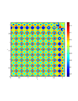
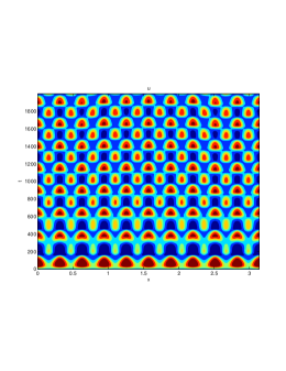
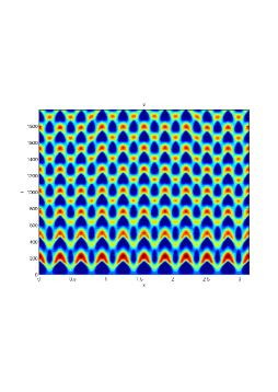
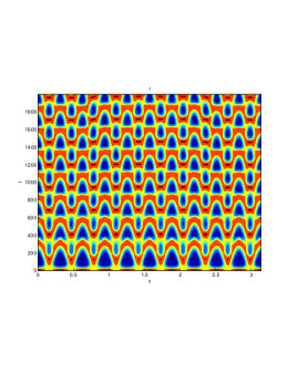
  • Turing instability exists in the model system (2)-(4), via theorem 5.3. Furthermore, the Allee threshold mm has a significant impact on the type of Turing patterns that form, see figures 3, 4, 5, 6, 7, 9.

2 Preliminary Estimates

2.1 Preliminaries

We now present various notations and definitions that will be used frequently. The usual norms in the spaces 𝕃p(Ω)\mathbb{L}^{p}(\Omega), 𝕃(Ω)\mathbb{L}^{\infty}(\Omega) and (Ω¯)\mathbb{C}\left(\overline{\Omega}\right) are respectively denoted by

upp=1|Ω|Ω|u(x)|p𝑑x,\left\|u\right\|_{p}^{p}\text{=}\frac{1}{\left|\Omega\right|}\int\limits_{\Omega}\left|u(x)\right|^{p}dx,
u=maxxΩ|u(x)|.\left\|u\right\|_{\infty}\text{=}\underset{x\in\Omega}{max}\left|u(x)\right|.

We define the following phase spaces

H=L2(Ω)×L2(Ω)×L2(Ω),H=L^{2}(\Omega)\times L^{2}(\Omega)\times L^{2}(\Omega),
E=H1(Ω)×H1(Ω)×H1(Ω),E=H^{1}(\Omega)\times H^{1}(\Omega)\times H^{1}(\Omega),
X=H2(Ω)×H2(Ω)×H2(Ω).X=H^{2}(\Omega)\times H^{2}(\Omega)\times H^{2}(\Omega).

We now recall the following lemma.

Lemma 2.1 (Uniform Gronwall Lemma)

Let β,ζ\beta,\zeta, and hh be nonnegative functions in Lloc1[0,;)L^{1}_{loc}[0,\infty;\mathbb{R}). Assume that β\beta is absolutely continuous on (0,)(0,\infty) and the following differential inequality is satisfied:

dβdtζβ+h,fort>0.\frac{d\beta}{dt}\leq\zeta\beta+h,\ \mbox{for}\ t>0. (5)

If there exists a finite time t1>0t_{1}>0 and some q>0q>0 such that

tt+qζ(τ)𝑑τA,tt+qβ(τ)𝑑τB,andtt+qh(τ)𝑑τC,\int^{t+q}_{t}\zeta(\tau)d\tau\leq A,\ \int^{t+q}_{t}\beta(\tau)d\tau\leq B,\ \mbox{and}\ \int^{t+q}_{t}h(\tau)d\tau\leq C, (6)

for any t>t1t>t_{1}, where A,BA,B, and CC are some positive constants, then

β(t)(Bq+C)eA,for  anyt>t1+q.\beta(t)\leq\left(\frac{B}{q}+C\right)e^{A},\ \mbox{for \ any}\ t>t_{1}+q. (7)

2.2 Uniform L2(Ω)L^{2}(\Omega) and H1(Ω)H^{1}(\Omega) estimates

In all estimates made hence forth the constants C,C1,C2,C3,CC,C_{1},C_{2},C_{3},C_{\infty} are generic constants, that can change in value from line to line, and sometimes within the same line if so required. Using positivity of the solution, and comparison arguments, one is easily able to prove global existence of classical solutions to system (2)-(4). We state the following result.

Proposition 2.2

All positive solutions of the system (2)-(4), with initial data in 𝕃(Ω)\mathbb{L}^{\infty}(\Omega) are classical and global.

See appendix 7.2 for the proof. Although we have global existence of classical via proposition 2.2, we can actually derive uniform L(Ω)L^{\infty}(\Omega) bounds, for initial data only in L2(Ω)L^{2}(\Omega). This will facilitate estimates required to show existence of bounded absorbing sets and the compactness of trajectories, which will lead to the existence of a global attractor in the product space L2(Ω)L^{2}(\Omega). Since the construction of global attractors require a Hilbert space setting, where the appropriate function spaces are the Hilbert spaces L2(Ω)L^{2}(\Omega) and Hs(Ω)H^{s}(\Omega), s=1,2s=1,2, we want to proceed by showing there is a weak solution in these function spaces. We then make estimates on this class of solutions, to proceed with the requisite analysis for the global attractors. We state the following theorem:

Theorem 2.3

Consider the three species food chain model described via (2)-(4). For any initial data (u0,v0,r0)(u_{0},v_{0},r_{0}) in L2(Ω)L^{2}(\Omega), and spatial dimension n=1,2,3n=1,2,3, there exists a global weak solution (u,v,r)(u,v,r) to the system, which becomes a strong solution and then a classical solution.

The proofs of proposition 2.2 and theorem 2.3 follow via remark 2.7 and the estimates referred to therein.

We state the following result next,

Lemma 2.4

Consider (u,v,r)(u,v,r) that are solutions to the diffusive three species food chain model described via (2)-(4), for any (u0,v0,r0)L2(Ω)(u_{0},v_{0},r_{0})\in L^{2}(\Omega), and spatial dimension n=1,2,3n=1,2,3, there exists a time t(u02,v02)t^{*}(||u_{0}||_{2},||v_{0}||_{2}) , and a constant CC independent of time, initial data and the allee threshold mm, and dependent only on the other parameters in (2)-(4), such that for any t>tt>t^{*} the following uniform estimates hold:

u22C,v22C,tt+1u22𝑑sC,tt+1v22𝑑sC,u22C,v22C.||u||^{2}_{2}\leq C,||v||^{2}_{2}\leq C,\int^{t+1}_{t}||\nabla u||^{2}_{2}ds\leq C,\int^{t+1}_{t}||\nabla v||^{2}_{2}ds\leq C,||\nabla u||^{2}_{2}\leq C,||\nabla v||^{2}_{2}\leq C. (8)

This follows easily via the estimates and methods of [20, 18, 19]. Note what differs here from [20, 18, 19] is the equation for rr, particularly due to a Allee effect now being modeled.

We now proceed with the estimate on rr. We multiply (4) by rr and integrate by parts to obtain

12ddtr22+d3r22+w3v+D3r44(c+mw3v+D3)r33.\frac{1}{2}\frac{d}{dt}||r||^{2}_{2}+d_{3}||\nabla r||^{2}_{2}+\frac{w_{3}}{||v||_{\infty}+D_{3}}||r||^{4}_{4}\leq\left(c+\frac{mw_{3}}{v+D_{3}}\right)||r||^{3}_{3}. (9)

Thus we obtain

12ddtr22+d3r22+cmr22+w3v+D3r44(c+mw3v+D3)r33.\frac{1}{2}\frac{d}{dt}||r||^{2}_{2}+d_{3}||\nabla r||^{2}_{2}+cm||r||^{2}_{2}+\frac{w_{3}}{||v||_{\infty}+D_{3}}||r||^{4}_{4}\leq\left(c+\frac{mw_{3}}{v+D_{3}}\right)||r||^{3}_{3}. (10)

We then use Hölder’s inequality followed by Young’s inequality to obtain

12ddtr22+d3r22+cmr22+w3v+D3r44,\displaystyle\frac{1}{2}\frac{d}{dt}||r||^{2}_{2}+d_{3}||\nabla r||^{2}_{2}+cm||r||^{2}_{2}+\frac{w_{3}}{||v||_{\infty}+D_{3}}||r||^{4}_{4},
w3v+D3r44+C1(v+D3+m4)|Ω|.\displaystyle\leq\frac{w_{3}}{||v||_{\infty}+D_{3}}||r||^{4}_{4}+C_{1}(||v||_{\infty}+D_{3}+m^{4})|\Omega|.

Thus we obtain

12ddtr22+cmr22C1(v+D3+m4)|Ω|,\frac{1}{2}\frac{d}{dt}||r||^{2}_{2}+cm||r||^{2}_{2}\leq C_{1}(||v||_{\infty}+D_{3}+m^{4})|\Omega|, (12)

which implies

r22ecmtr022+C1(v+D3+m4)|Ω|cm.||r||^{2}_{2}\leq e^{-cmt}||r_{0}||^{2}_{2}+\frac{C_{1}(||v||_{\infty}+D_{3}+m^{4})|\Omega|}{cm}. (13)

We now use the estimate for v||v||_{\infty} via (27) (which does not depend on rr see remark 2.8) to obtain the following estimates for rr,

r221+C1(C+D3+m4)|Ω|cm,fort>max(t+1,ln(r022)cm).||r||^{2}_{2}\leq 1+\frac{C_{1}(C+D_{3}+m^{4})|\Omega|}{cm},\ \mbox{for}\ t>\max\left(t^{*}+1,\frac{\ln(||r_{0}||^{2}_{2})}{cm}\right). (14)

Integrating (7.4) in the time interval [t,t+1][t,t+1] we obtain

tt+1r22𝑑s1+C1(C+D3+m4)|Ω|cm+2|Ω|14(c+w4D3)(w4D3)14,\int^{t+1}_{t}||\nabla r||^{2}_{2}ds\leq 1+\frac{C_{1}(C+D_{3}+m^{4})|\Omega|}{cm}+2|\Omega|^{\frac{1}{4}}\left(c+\frac{w_{4}}{D_{3}}\right)\left(\frac{w_{4}}{D_{3}}\right)^{\frac{1}{4}}, (15)

for t>max(t+1,ln(r022)cm)t>\max\left(t^{*}+1,\frac{\ln(||r_{0}||^{2}_{2})}{cm}\right).

Here, C,C1C,C_{1} do not depend on mm.

Remark 2.5

What we notice is that the estimate via (14), (15) depend singularly on mm. That is they yield no information, if we try to pass to the limit as m0m\rightarrow 0

We now estimate the gradient of rr. See the appendix 7.3 for details. What the standard analysis in appendix 7.3 shows, is that we have an estimate of the form

lim suptr22C,\mathop{\limsup}_{t\rightarrow\infty}||\nabla r||^{2}_{2}\leq C, (16)
Remark 2.6

The constant CC in (16) is independent of time and initial conditions, but depend singularly on mm. In our estimates we apply the uniform Gronwall lemma which requires us to use the estimate via (15). This also depends singularly on mm, thus the estimate (16) is uniform with respect to time and initial data but depend singularly on mm.

Remark 2.7

The uniform H1(Ω)H^{1}(\Omega) estimates via lemma 2.4 and (95) give us uniform L6(Ω)L^{6}(\Omega) bounds in 3\mathbb{R}^{3}. We can now prove the reaction terms are in Lp(Ω)L^{p}(\Omega) for p>32p>\frac{3}{2}. It suffices to show that

uu2w1uvu+v2Cu42C,||u-u^{2}-w_{1}\frac{uv}{u+v}||_{2}\leq C||u||^{2}_{4}\leq C, (17)
a2v+w2uvu+vw3(vrv+r)2Cv2C,||-a_{2}v+w_{2}\frac{uv}{u+v}-w_{3}\left(\frac{vr}{v+r}\right)||_{2}\leq C||v||_{2}\leq C, (18)
r(rm)(cw4rv+D3)2Cr63C.||r\big{(}{{r-m}}\big{)}\bigg{(}c-\frac{w_{4}r}{v+D_{3}}\bigg{)}||_{2}\leq C||r||^{3}_{6}\leq C. (19)

But the above follows via the uniform L6(Ω)L^{6}(\Omega) bounds on u,v,ru,v,r. This proves proposition 2.2. Furthermore the estimate via (16) and lemma 2.4 allow us to derive the appropriate L2(Ω)L^{2}(\Omega) and H1(Ω)H^{1}(\Omega) bounds on a Galerkin truncation of (2)-(4), extract appropriate subsequebces and pass to the limit as is standard [27, 22], to prove theorem 2.3.

2.3 Uniform in the parameter mm L2(Ω)L^{2}(\Omega) and H1(Ω)H^{1}(\Omega) estimates for rr

Note the estimates via (14), (16) are singular in mm. This causes extensive difficulties if we try to pass to the limit as m0m\rightarrow 0, hence making it difficult to prove upper semicontinuity. Our next goal is to derive uniform in mm estimate on rr. These are derived in detail in the appendix 7.4. However, the key estimate derived therein is

r22CKeKCK,fort>t1=t0+1.\displaystyle||\nabla r||^{2}_{2}\leq C_{K}e^{KC_{K}},\ \mbox{for}\ t>t_{1}=t_{0}+1. (20)

Here CK,KC_{K},K are independent of mm. Thus the H1(Ω)H^{1}(\Omega) estimate for rr can be made independent of mm.

2.4 Uniform H2(Ω)H^{2}(\Omega) estimates

We will now estimate the H2(Ω)H^{2}(\Omega) norms of the solution. We rewrite (2) as

utd1Δu=uu2w1(uvu+v).u_{t}-d_{1}\Delta u=u-u^{2}-w_{1}\left(\frac{uv}{u+v}\right).

We square both sides of the equation and integrate by parts over Ω\Omega to obtain

ut22+d1Δu22+ddtu22,\displaystyle||u_{t}||^{2}_{2}+d_{1}||\Delta u||^{2}_{2}+\frac{d}{dt}||\nabla u||^{2}_{2},
=\displaystyle= (uu2w1(uvu+v))22,\displaystyle\left\|\left(u-u^{2}-w_{1}\left(\frac{uv}{u+v}\right)\right)\right\|_{2}^{2},
\displaystyle\leq C(u22+(w1)2u22+u44)C.\displaystyle C\left(||u||^{2}_{2}+(w_{1})^{2}||u||^{2}_{2}+||u||^{4}_{4}\right)\leq C.

This result follows by the embedding of H1(Ω)L4(Ω)L2(Ω)H^{1}(\Omega)\hookrightarrow L^{4}(\Omega)\hookrightarrow L^{2}(\Omega). Therefore, we obtain

ut22+d1Δu22+ddtu22C(u22+(w1)2u22+u44)C.||u_{t}||^{2}_{2}+d_{1}||\Delta u||^{2}_{2}+\frac{d}{dt}||\nabla u||^{2}_{2}\leq C\left(||u||^{2}_{2}+(w_{1})^{2}||u||^{2}_{2}+||u||^{4}_{4}\right)\leq C.

We now make uniform in time estimates of the higher order terms. Integrating the estimates of (2.4) in the time interval [T,T+1][T,T+1], for T>tT>t^{*}

TT+1ut22𝑑tC1,TT+1Δu22𝑑tC2.\int^{T+1}_{T}||u_{t}||^{2}_{2}dt\leq C_{1},\ \int^{T+1}_{T}||\Delta u||^{2}_{2}dt\leq C_{2}.

Similarly we adopt the same procedure for vv to obtain

TT+1vt22𝑑tC1,TT+1Δv22𝑑tC2.\int^{T+1}_{T}||v_{t}||^{2}_{2}dt\leq C_{1},\ \int^{T+1}_{T}||\Delta v||^{2}_{2}dt\leq C_{2}.

Next, consider the gradient of (2). Following the same technique as in deriving (2.4) we obtain for the left hand side

ut22+d1(Δu)22+ddtΔu22+ΩΔuutndS,\displaystyle||\nabla u_{t}||^{2}_{2}+d_{1}||\nabla(\Delta u)||^{2}_{2}+\frac{d}{dt}||\Delta u||^{2}_{2}+\int_{\partial\Omega}\Delta u\nabla u_{t}\cdot\textbf{n}dS,
=ut22+d1(Δu)22+ddtΔu22+ΩΔut(un)𝑑S,\displaystyle=||\nabla u_{t}||^{2}_{2}+d_{1}||\nabla(\Delta u)||^{2}_{2}+\frac{d}{dt}||\Delta u||^{2}_{2}+\int_{\partial\Omega}\Delta u\frac{\partial}{\partial t}(\nabla u\cdot\textbf{n})dS,
=ut22+d1(Δu)22+ddtΔu22.\displaystyle=||\nabla u_{t}||^{2}_{2}+d_{1}||\nabla(\Delta u)||^{2}_{2}+\frac{d}{dt}||\Delta u||^{2}_{2}. (21)

This follows via the boundary condition. Thus we have

ut22+d1(Δu)22+ddtΔu22,\displaystyle||\nabla u_{t}||^{2}_{2}+d_{1}||\nabla(\Delta u)||^{2}_{2}+\frac{d}{dt}||\Delta u||^{2}_{2},
=((uu2w1(uvu+v)))2,\displaystyle=\left(\nabla(u-u^{2}-w_{1}\left(\frac{uv}{u+v}\right))\right)^{2},
C(u44+v44+Δu24+v22+u22).\displaystyle\leq C(||u||^{4}_{4}+||v||^{4}_{4}+||\Delta u||^{4}_{2}+||\nabla v||^{2}_{2}+||\nabla u||^{2}_{2}). (22)

This follows via Young’s inequality with epsilon, as well as the embedding of H2(Ω)W1,4(Ω)H1(Ω)H^{2}(\Omega)\hookrightarrow W^{1,4}(\Omega)\hookrightarrow H^{1}(\Omega). This implies that

ddtΔu22CΔu24+C(u44+v44+v22+u22).\frac{d}{dt}||\Delta u||^{2}_{2}\leq C||\Delta u||^{4}_{2}+C(||u||^{4}_{4}+||v||^{4}_{4}+||\nabla v||^{2}_{2}+||\nabla u||^{2}_{2}).

We now use the uniform Gronwall lemma with

β(t)=Δu22,ζ(t)=Δu22,h(t)=C(u44+v44+v22+u22),q=1,\beta(t)=||\Delta u||^{2}_{2},\ \zeta(t)=||\Delta u||^{2}_{2},\ h(t)=C(||u||^{4}_{4}+||v||^{4}_{4}+||\nabla v||^{2}_{2}+||\nabla u||^{2}_{2}),~~q=1,

to obtain

Δu2C,Δv2C,fort>t+1.||\Delta u||_{2}\leq C,\ ||\Delta v||_{2}\leq C,\ \mbox{for}\ t>t^{*}+1.

The estimate for vv is derived similarly.

Remark 2.8

It is critical to notice that the estimate for Δv2||\Delta v||_{2} does not involve rr. This is because in order to derive it, we adopt same procedure as in (2.4), instead for the vv equation, and square both sides to proceed. Therein notice that the term involving rr, vrv+r\frac{vr}{v+r} can be estimated as vrv+r2Crv+rv2C1v2||\frac{vr}{v+r}||_{2}\leq C||\frac{r}{v+r}||_{\infty}||v||_{2}\leq C_{1}||v||_{2}. So the right hand side has no dependence on rr.

In order to estimate the H2(Ω)H^{2}(\Omega) norm of rr we proceed similarly to obtain

rt22+d3Δr22+ddtr22\displaystyle||r_{t}||^{2}_{2}+d_{3}||\Delta r||^{2}_{2}+\frac{d}{dt}||\nabla r||^{2}_{2} =\displaystyle= ((c+mw4v+D3)r2w4v+D3r3mcr)22,\displaystyle\left\|\left(\left(c+\frac{mw_{4}}{v+D_{3}}\right)r^{2}-\frac{w_{4}}{v+D_{3}}r^{3}-mcr\right)\right\|_{2}^{2},
\displaystyle\leq C(r22+r44)+r66,\displaystyle C\left(||r||^{2}_{2}+||r||^{4}_{4}\right)+||r||^{6}_{6},
\displaystyle\leq C(r22)3.\displaystyle C\left(||\nabla r||^{2}_{2}\right)^{3}.

We now make uniform in time estimates of the higher order terms. Integrating the estimates of (2.4) in the time interval [T,T+1][T,T+1], for T>t1T>t_{1}, and using the estimates via (7.4) yields

TT+1rt22𝑑tC1,TT+1Δr22𝑑tC2.\int^{T+1}_{T}||r_{t}||^{2}_{2}dt\leq C_{1},\ \int^{T+1}_{T}||\Delta r||^{2}_{2}dt\leq C_{2}.

Next, consider the gradient of (4). Following the same technique as in deriving (2.4) we obtain

rt22+d3(Δr)22+ddtΔr22\displaystyle||\nabla r_{t}||^{2}_{2}+d_{3}||\nabla(\Delta r)||^{2}_{2}+\frac{d}{dt}||\Delta r||^{2}_{2} =(((c+mw4v+D3)r2w4v+D3r3mcr))2,\displaystyle=\left(\nabla\left(\left(c+\frac{mw_{4}}{v+D_{3}}\right)r^{2}-\frac{w_{4}}{v+D_{3}}r^{3}-mcr\right)\right)^{2},
C(r22)2.\displaystyle\leq C\left(||\nabla r||^{2}_{2}\right)^{2}.

This yields

ddtΔr22C(r22)2(Δr22)+C2(r22)2.\frac{d}{dt}||\Delta r||^{2}_{2}\leq C\left(||\nabla r||^{2}_{2}\right)^{2}\left(||\Delta r||^{2}_{2}\right)+C_{2}\left(||r||^{2}_{2}\right)^{2}. (25)

We can now use the estimates via (99), (7.4) in conjunction with the uniform Gronwall lemma to yield a uniform bound on Δr2||\Delta r||_{2}. Thus, via elliptic regularity,

uH2(Ω)C,vH2(Ω)C,rH2(Ω)Cfort>max(t1+1,t+1).||u||_{H^{2}(\Omega)}\leq C,\ ||v||_{H^{2}(\Omega)}\leq C,\ ||r||_{H^{2}(\Omega)}\ \leq C\ \mbox{for}\ t>\max(t_{1}+1,t^{*}+1). (26)

Since H2(Ω)L(Ω)H^{2}(\Omega)\hookrightarrow L^{\infty}(\Omega) in 2\mathbb{R}^{2} and 3\mathbb{R}^{3}, the following estimate is valid in 2\mathbb{R}^{2} and 3\mathbb{R}^{3}

uC,vC,rCfort>max(t1+1,t+1).||u||_{\infty}\leq C,\ ||v||_{\infty}\leq C,\ ||r||_{\infty}\leq C\ \mbox{for}\ t>\max(t_{1}+1,t^{*}+1). (27)

3 Long Time Dynamics

3.1 Existence of global attractor

In this section we prove the existence of a (H,H)(H,H) global attractor for system (2)-(4), which is subsequently demonstrated to be a (H,E)(H,E) attractor. We now state the following theorem,

Theorem 3.1

Consider the reaction diffusion equation described via (2)-(4) where Ω\Omega is of spatial dimension n=1,2,3n=1,2,3. There exists a (H,H)(H,H) global attractor 𝒜\mathcal{A} for the system. This is compact and invariant in HH, and it attracts all bounded subsets of HH in the HH metric.

proof We have shown that the system is well posed via theorems 2.3. Thus there exists a well defined semigroup {S(t)}t0:HH\left\{S(t)\right\}_{t\geq 0}:H\rightarrow H. The estimates derived in Lemma 2.4 demonstrate the existence of bounded absorbing sets in HH and EE. Thus given a sequence {u0,n}n=1\left\{u_{0,n}\right\}^{\infty}_{n=1}, that is bounded in L2(Ω)L^{2}(\Omega), we know that for t>tt>t^{*},

S(t)(u0,n)BH1(Ω).S(t)(u_{0,n})\subset B\subset H^{1}(\Omega). (28)

Here BB is the bounded absorbing set in H1(Ω)H^{1}(\Omega) from lemma 2.4. Now for n large enough tn>tt_{n}>t^{*}, thus for such tnt_{n} we have

S(tn)(u0,n)BH1(Ω).S(t_{n})(u_{0,n})\subset B\subset H^{1}(\Omega). (29)

This implies that we have the following uniform bound,

S(tn)(u0,n)H1(Ω)C,||S(t_{n})(u_{0,n})||_{H^{1}(\Omega)}\leq C, (30)

This implies via standard functional analysis theory, see [27], the existence of a subsequence still labeled S(tn)(u0,n)S(t_{n})(u_{0,n}) such that

S(tn)(u0,n)uinH1(Ω),S(t_{n})(u_{0,n})\rightharpoonup u\ \mbox{in}\ H^{1}(\Omega), (31)

Which implies via the compact Sobolev embedding of

EH,E\hookrightarrow H, (32)

that

S(tn)(u0,n)uinL2(Ω).S(t_{n})(u_{0,n})\rightarrow u\ \mbox{in}\ L^{2}(\Omega). (33)

This yields the asymptotic compactness of the semigroup {S(t)}t0\left\{S(t)\right\}_{t\geq 0} in HH. The convergences for the v,rv,r components follow similarly. The theorem is now proved. \square

Next we can state the following theorem

Theorem 3.2

Consider the reaction diffusion equation described via (2)-(4) where Ω\Omega is of spatial dimension n=1,2,3n=1,2,3. There exists a (H,E)(H,E) global attractor 𝒜\mathcal{A} for the system. This is compact and invariant in HH, and it attracts all bounded subsets of HH in the EE metric.

proof The proof essentially follows verbatim theorem 3.1. The existence of a bounded absorbing set in EE follows from lemma 2.4. In order to prove the asymptotic compactness in EE we use the uniform H2(Ω)H^{2}(\Omega) estimates in (26), and the compact Sobolev embedding of H2(Ω)H1(Ω)H^{2}(\Omega)\hookrightarrow H^{1}(\Omega). \square

3.2 Upper-semicontinuity of Global attractor with respect to the Allee parameter mm

Here we state and prove the main semicontinuity result. This result follows via a series of estimates, and theorems, all of which we derive for the reader in appendix 7.5

Theorem 3.3

Consider the reaction diffusion equation described via (2)-(4) where Ω\Omega is of spatial dimension n=1,2,3n=1,2,3. Given a set of positive parameters excluding mm, the family of global attractors is upper semicontinuous with respect to the Allee threshold m0m\geq 0 as it converges to zero. That is

distE(𝒜m,𝒜0)0,asm0+.dist_{E}(\mathcal{A}_{m},\mathcal{A}_{0})\rightarrow 0,\ \mbox{as}\ m\rightarrow 0^{+}. (34)
Proof 3.4

We know that for ϵ>0\epsilon>0, the global attractor 𝒜0\mathcal{A}_{0} for the reaction diffusion equation described via (2)-(4) attracts 𝒰\mathcal{U}. This follows via theorems 7.6, 7.7 and 7.9. Thus there exists a finite time tϵ>0t_{\epsilon}>0, such that

S0(tϵ)𝒰𝒩E(𝒜0,ϵ2).S_{0}(t_{\epsilon})\mathcal{U}\subset\mathcal{N}_{E}(\mathcal{A}_{0},\frac{\epsilon}{2}). (35)

Here, 𝒩E(𝒜0,ϵ2)\mathcal{N}_{E}(\mathcal{A}_{0},\frac{\epsilon}{2}) is the ϵ2\frac{\epsilon}{2} ball of 𝒜0\mathcal{A}_{0} in the space EE. Now we also know by the uniform convergence theorem, theorem 7.10 that there exists a mϵ(0,1]m_{\epsilon}\in(0,1] such that

supg0𝒰Sm(tϵ)g0S0(tϵ)g0Eϵ2,foranymmϵ.\sup_{g_{0}\in\mathcal{U}}||S_{m}(t_{\epsilon})g_{0}-S_{0}(t_{\epsilon})g_{0}||_{E}\leq\frac{\epsilon}{2},\ \mbox{for}\ \mbox{any}\ m\in m_{\epsilon}. (36)

Since we know 𝒜m\mathcal{A}_{m} is invariant we have

𝒜m=Sm(tϵ)𝒜mSm(tϵ)𝒰𝒩E(S0(tϵ)𝒰,ϵ2)𝒩E(𝒜0,ϵ).\mathcal{A}_{m}=S_{m}(t_{\epsilon})\mathcal{A}_{m}\subset S_{m}(t_{\epsilon})\mathcal{U}\subset\mathcal{N}_{E}(S_{0}(t_{\epsilon})\mathcal{U},\frac{\epsilon}{2})\subset\mathcal{N}_{E}(\mathcal{A}_{0},\epsilon). (37)

Thus one obtains the upper semicontinuity,

distE(𝒜m,𝒜0)0,asm0+.dist_{E}(\mathcal{A}_{m},\mathcal{A}_{0})\rightarrow 0,\ \mbox{as}\ m\rightarrow 0^{+}. (38)

This proves the theorem.

3.3 Computing the decay rate with respect to the Allee threshold parameter mm

In the previous subsection 3.2, the role of the Allee threshold parameter mm on the long time dynamics of system (2)-(4) is explored. Theorem 3.3 shows that the global attractors 𝒜m\mathcal{A}_{m} converge to 𝒜0\mathcal{A}_{0} in the H1(Ω)H^{1}(\Omega) norm, as mm decreases to zero. It is also seen how changing mm effects the Turing dynamics in subsection 5. Theorem 3.3 is a purely theoretical result. It gives no information as to the exact decay rate in terms of the parameter mm. In general, there are no results in the literature to estimate this decay rate. We now aim to examine the role of mm with respect to convergence, as mm decreases to zero as discussed earlier. We aim to explicitly find the decay rate of 𝒜m\mathcal{A}_{m} to a target attractor 𝒜0\mathcal{A}_{0} (that is when m=0m=0). We choose Turing patterns as the state of interest. In particular the numerical scheme discussed in 5 was employed, and the Turing patterns at an extended time are examined. The goal is to gather numerical evidence as to the dependence on mm with respect to the convergence rate,

UmU0H1(Ω)\displaystyle\|U_{m}-U_{0}\|_{H^{1}(\Omega)} <\displaystyle< Cmγ,\displaystyle Cm^{\gamma}, (39)

where U0=(u,v0,r0)U_{0}=(u_{,}v_{0},r_{0}) is the solution for m=0m=0, Um=(um,vm,rm)U_{m}=(u_{m},v_{m},r_{m}) is the solution for any given value of mm, and both CC and γ\gamma are constants.

The numerical approximation for the case m=0m=0 was established at the scaled time, t=10,000t=10,000. The approximations, um(x,t)u_{m}(x,t), vm(x,t)v_{m}(x,t), and rm(x,t)r_{m}(x,t), were then established for a range of values of mm with 121 equally spaced values from 0 to 0.0035. The approximation for each value of mm was established up to t=10,000t=10,000, and it was determined that for each value of mm in this range a fixed spatial pattern was found. The H1(Ω)H^{1}(\Omega) errors for the numerical approximation were then calculated with respect to the m=0m=0 case,

um(,10,000)u0(,10,000)H1(Ω),\displaystyle\|u_{m}(\cdot,10,000)-u_{0}(\cdot,10,000)\|_{H^{1}(\Omega)},
vm(,10,000)v0(,10,000)H1(Ω),\displaystyle\|v_{m}(\cdot,10,000)-v_{0}(\cdot,10,000)\|_{H^{1}(\Omega)},
rm(,10,000)r0(,10,000)H1(Ω).\displaystyle\|r_{m}(\cdot,10,000)-r_{0}(\cdot,10,000)\|_{H^{1}(\Omega)}.
Refer to caption
Figure 1: The H1(Ω)H^{1}(\Omega) errors for the differences um(,10,000)u0(,10,000)\|u_{m}(\cdot,10,000)-u_{0}(\cdot,10,000)\|, vm(,10,000)v0(,10,000)\|v_{m}(\cdot,10,000)-v_{0}(\cdot,10,000)\|, and rm(,10,000)r0(,10,000)\|r_{m}(\cdot,10,000)-r_{0}(\cdot,10,000)\| are shown for a range of values of mm. The solid line is the linear least squares regression line.
Refer to caption
Figure 2: The H1(Ω)H^{1}(\Omega) errors for the differences um(,10,000)u0(,10,000)\|u_{m}(\cdot,10,000)-u_{0}(\cdot,10,000)\|, vm(,10,000)v0(,10,000)\|v_{m}(\cdot,10,000)-v_{0}(\cdot,10,000)\|, and rm(,10,000)r0(,10,000)\|r_{m}(\cdot,10,000)-r_{0}(\cdot,10,000)\| are shown for a range of values of mm but are plotted in a log log format. The solid line is the linear least squares regression line for the log-log data.

The errors are shown in Figure 1 and Figure 2. The first figure, Figure 1, shows the raw errors, and the second figure, Figure 2, shows the errors as a log-log plot. A linear least squares fit for the data was also calculated, and the best fit straight line is shown on both plots. In both cases the close linear fit for larger values of mm contribute to strong, positive correlations in the data. However, for smaller values mm the log-log data moves away from a straight line. For the smaller values of mm the errors in the numerical approximation are of the same order as the error in the H1(Ω)H^{1}(\Omega) norm, and the data no longer follows the same trend.

Examining the errors for umu_{m}, the correlation for the raw data is 0.99995, and the data reveals a strong, positive linear relationship. In this scenario, it is assumed that the value of γ\gamma in equation (39) is one. The approximation for the slope of the raw data gives an estimate of 20.6 with a 95% confidence interval between 20.6215 and 20.6206. The 95% confidence interval for the intercept is between -5.1E-5 and -9.0E-4. Due to the large number of samples, the error in the confidence interval is very small, but the estimate for the parameter is close to zero.

Examining the errors for the log of the errors correlation is 0.993 for the log-log data. The approximation for the slope of the log-log data gives an estimate of 1.003 with a 95% confidence interval between 0.72 and 1.28. The 95% confidence interval for the intercept is between 2.7 and 3.3. Note that the value of one is within the confidence interval making it difficult to claim that the relationship is not linear. The estimate for the slope, in fact, is very close to one indicating that the value of γ\gamma in equation (39) is close to one.

4 Overexploitation Phenomenon

Overexploitation refers to the phenomenon where excessive harvesting of a species can result in its extinction. This finds applications in conservation, biodiversity, cascade control and so on. Although there is a fair amount of literature on this in two species models [32], it is much less studied in three species models. To begin, we state the following theorem

Theorem 4.1 (Middle predator and Allee effect mediated overexploitation)

Consider (u,v,r)(u,v,r) that are solutions to the diffusive three species food chain model described via (2)-(4). If w1>a2+1+w3w_{1}>a_{2}+1+w_{3}, then for any given initial prey density u0u_{0} there exists a threshold M1=1αu0pM_{1}=\frac{1}{\alpha}||u_{0}||_{p}, s.t if M1<v0pM_{1}<||v_{0}||_{p} and r0<min(m,cD3w4)||r_{0}||_{\infty}<\min(m,\frac{cD_{3}}{w_{4}}), then (u,v,r)(0,0,0)(u,v,r)\rightarrow(0,0,0) uniformly for xΩ¯x\in\bar{\Omega} as tt\rightarrow\infty.

proof: We begin by looking at the equation for uu, and following the ideas in [12]

ut=d1Δu+uu2w1uvu+v=d1Δu+uu2w1uuv+1.\frac{\partial u}{\partial t}=d_{1}\Delta u+u-u^{2}-w_{1}\frac{uv}{u+v}=d_{1}\Delta u+u-u^{2}-w_{1}\frac{u}{\frac{u}{v}+1}. (40)

We will claim that for all tt, uv<α||\frac{u}{v}||_{\infty}<\alpha, and limtup0\lim_{t\rightarrow\infty}||u||_{p}\rightarrow 0, p\forall p, if u0pv0p<α\frac{||u_{0}||_{p}}{||v_{0}||_{p}}<\alpha. If not there exists a first time t1t_{1} s.t., upvp<α\frac{||u||_{p}}{||v||_{p}}<\alpha on t[0,t1]t\in[0,t_{1}] and u(t1)pv(t1)p=α\frac{||u(t_{1})||_{p}}{||v(t_{1})||_{p}}=\alpha.

Due to w1>a2+1+w3w_{1}>a_{2}+1+w_{3}, there exists an α\alpha s.t w11+α=1+a2+w3\frac{w_{1}}{1+\alpha}=1+a_{2}+w_{3}, thus

ut=d1Δu+uu2w1uuv+1\displaystyle\frac{\partial u}{\partial t}=d_{1}\Delta u+u-u^{2}-w_{1}\frac{u}{\frac{u}{v}+1} d1Δu+uw1uα+1,\displaystyle\leq d_{1}\Delta u+u-w_{1}\frac{u}{\alpha+1}, (41)
=d1Δu+uua2uw3u,\displaystyle=d_{1}\Delta u+u-u-a_{2}u-w_{3}u,
=d1Δu(a2+w3)u.\displaystyle=d_{1}\Delta u-(a_{2}+w_{3})u.

Thus uu satisfies

upu0pe(a2+w3)t.||u||_{p}\leq||u_{0}||_{p}e^{-(a_{2}+w_{3})t}. (42)

This easily follows via multiplying (2) by |u|p1|u|^{p-1}, and integrating by parts. We also notice that the v~\tilde{v} solving the following equation, with v~0=supv0(x)\tilde{v}_{0}=\sup v_{0}(x), is a super solution to (3)

v~t=(a2+w3)v~.\frac{\partial\tilde{v}}{\partial t}=-(a_{2}+w_{3})\tilde{v}. (43)

Multiplying through by |v|p1|v|^{p-1}, and integrating by parts yields

vpv0pe(a2+w3)t.||v||_{p}\geq||v_{0}||_{p}e^{-(a_{2}+w_{3})t}. (44)

This implies

upvpu0pv0p<α.\frac{||u||_{p}}{||v||_{p}}\leq\frac{||u_{0}||_{p}}{||v_{0}||_{p}}<\alpha. (45)

This implies a contradiction. Thus limtup0\lim_{t\rightarrow\infty}||u||_{p}\rightarrow 0, which implies uniform convergence of a subsequence, say unju_{n_{j}} to 0 (where unu_{n} is a Galerkin truncation of uu and standard theory is adopted [22]), and by uniqueness of solutions, u0u\rightarrow 0 uniformly, as tt\rightarrow\infty. This reduces the vv equation to

vt=d2Δva2vw3(vrv+r)d2Δva2v,\frac{\partial v}{\partial t}=d_{2}\Delta v-a_{2}v-w_{3}\left(\frac{vr}{v+r}\right)\leq d_{2}\Delta v-a_{2}v, (46)

and it is easy to see that v0v\rightarrow 0 uniformly, as tt\rightarrow\infty.

Now the rr equation reduces to

rt=d3Δr+r(rm)(cw4rD3),\frac{\partial r}{\partial t}=d_{3}\Delta r+r\big{(}{{r-m}}\big{)}\bigg{(}c-\frac{w_{4}r}{D_{3}}\bigg{)}, (47)

and if r0<min(m,cD3w4)||r_{0}||_{\infty}<\min(m,\frac{cD_{3}}{w_{4}}) standard analysis yields

r0r\rightarrow 0 uniformly.

This proves the theorem.

\square

Remark 4.2

Note, in the three species food chain model (2)-(4), overexploitation has to be middle predator mediated, and also depends on the allele threshold. Clearly if r0p>max(m,cD3w4)||r_{0}||_{p}>\max(m,\frac{cD_{3}}{w_{4}}), or cD3w4<r0p<m\frac{cD_{3}}{w_{4}}<||r_{0}||_{p}<m, or cD3w4>r0p>m\frac{cD_{3}}{w_{4}}>||r_{0}||_{p}>m, rr cannot go extinct.

Also, if the attack rate of the top predator rr is large enough, it could cause vv to go extinct, before uu does. Once vv goes extinct u1u\rightarrow 1, again prohibiting overexploitation.

Theorem 4.3 (Top predator mediated overexploitation avoidance)

Consider (u,v,r)(u,v,r) that are solutions to the diffusive three species food chain model described via (2)-(4). If w3>w2+1+w1w_{3}>w_{2}+1+w_{1}, then for any given initial prey density u0u_{0} there exists a threshold M2=1α1r0pM_{2}=\frac{1}{\alpha_{1}}||r_{0}||_{p}, s.t if max(M2,m,cD3w4)<r0p\max\left(M_{2},m,\frac{cD_{3}}{w_{4}}\right)<||r_{0}||_{p} then (u,v,r)(1,0,r)(u,v,r)\rightarrow(1,0,r^{*}) uniformly as tt\rightarrow\infty.

proof: We first derive a lower bound on uu. Trivially we have u1||u||_{\infty}\leq 1. Now

utu2w1vuv+uuw1u.\frac{\partial u}{\partial t}\geq-u^{2}-w_{1}\frac{vu}{v+u}\geq-u-w_{1}u. (48)

This yields

upu0pe(1+w1)t.||u||_{p}\geq||u_{0}||_{p}e^{-(1+w_{1})t}. (49)

Next we will claim that for all tt, vr<α1||\frac{v}{r}||_{\infty}<\alpha_{1}, and limtvp0\lim_{t\rightarrow\infty}||v||_{p}\rightarrow 0, p\forall p, if v0pr0p<α1\frac{||v_{0}||_{p}}{||r_{0}||_{p}}<\alpha_{1}. If not there exists a first time t2t_{2} s.t., vprp<α1\frac{||v||_{p}}{||r||_{p}}<\alpha_{1} on t[0,t2]t\in[0,t_{2}] and u(t2)pv(t2)p=α1\frac{||u(t_{2})||_{p}}{||v(t_{2})||_{p}}=\alpha_{1}.

Due to the choice of w3>w2+1+w1w_{3}>w_{2}+1+w_{1}, there exists an α1\alpha_{1} s.t w31+α1=1+w2+w1\frac{w_{3}}{1+\alpha_{1}}=1+w_{2}+w_{1}, thus

vt\displaystyle\frac{\partial v}{\partial t} =d2Δva2v+w2vuv+uw3vvr+1,\displaystyle=d_{2}\Delta v-a_{2}v+w_{2}\frac{vu}{v+u}-w_{3}\frac{v}{\frac{v}{r}+1},
d2Δva2v+w2vw31+α1v,\displaystyle\leq d_{2}\Delta v-a_{2}v+w_{2}v-\frac{w_{3}}{1+\alpha_{1}}v,
=d2Δva2v+w2v(1+w2+w1)v.\displaystyle=d_{2}\Delta v-a_{2}v+w_{2}v-(1+w_{2}+w_{1})v.

Thus vv satisfies

vpv0pe(a2+1+w3)t.||v||_{p}\leq||v_{0}||_{p}e^{-(a_{2}+1+w_{3})t}. (51)

By the restriction on r0r_{0}, we see that trivially rmr\rightarrow m or rcD3w3r\rightarrow\frac{cD_{3}}{w_{3}}. This implies

vprpv0pr0p<α1.\frac{||v||_{p}}{||r||_{p}}\leq\frac{||v_{0}||_{p}}{||r_{0}||_{p}}<\alpha_{1}. (52)

This implies a contradiction. Thus limtvp0\lim_{t\rightarrow\infty}||v||_{p}\rightarrow 0, which implies uniform convergence to 0 of a subsequence, say vnjv_{n_{j}} (where vnv_{n} is a Galerkin truncation of vv and standard theory is adopted [22]), and by uniqueness v0v\rightarrow 0 uniformly as tt\rightarrow\infty. Looking at the decay rate for vv, we see it converges to 0 faster than uu, so u>0u>0, when v0v\rightarrow 0 uniformly, and so then the uu equation reduces to

ut=d1Δu+uu2,\frac{\partial u}{\partial t}=d_{1}\Delta u+u-u^{2}, (53)

and we know via standard theory that now u1u\rightarrow 1 uniformly.

This proves the theorem. \square

Remark 4.4

This also happens if cD3w4<r0<m\frac{cD_{3}}{w_{4}}<||r_{0}||_{\infty}<m, or cD3w4>r0>m\frac{cD_{3}}{w_{4}}>||r_{0}||_{\infty}>m.

The following lemma describes persistence in the top predator.

Lemma 4.5 (Persistence in top predator)

Consider (u,v,r)(u,v,r) that are solutions to the diffusive three species food chain model described via (2)-(4). If min(m,cD3w4)<r0\min(m,\frac{cD_{3}}{w_{4}})<||r_{0}||_{\infty}, then rmax(m,cD3w4)r\rightarrow\max(m,\frac{cD_{3}}{w_{4}}) uniformly as tt\rightarrow\infty, hence persists.

proof: Note cw4rv+D3>cw4rD3c-\frac{w_{4}r}{v+D_{3}}>c-\frac{w_{4}r}{D_{3}}, due to positivity of r,vr,v. Thus we can compare the solution of (4) to the solution of the ODE

dr~dt=r~(r~m)(cw4r~v+D3),\frac{d\tilde{r}}{dt}=\tilde{r}(\tilde{r}-m)\bigg{(}c-\frac{w_{4}\tilde{r}}{v+D_{3}}\bigg{)}, (54)

with r~0=min(r0(x))>min(m,cD3w4)\tilde{r}_{0}=\min(r_{0}(x))>\min(m,\frac{cD_{3}}{w_{4}}). Clearly r~max(m,cD3w4)\tilde{r}\rightarrow\max(m,\frac{cD_{3}}{w_{4}}) as tt\rightarrow\infty, and since rr solving (4) is a supersolution to r~\tilde{r} solving (54), we have lim inftminΩ¯(r(x,t)max(m,cD3w4)\liminf_{t\rightarrow\infty}\min_{\bar{\Omega}}(r(x,t)\geq\max(m,\frac{cD_{3}}{w_{4}}).

\square

Remark 4.6

In the event that there is no Allee effect, or m=0m=0, rcD3w4r\rightarrow\frac{cD_{3}}{w_{4}} uniformly as tt\rightarrow\infty, hence always persists, independent of all other parameters or initial data (u0,v0,r0)(u_{0},v_{0},r_{0}). Thus in a three species system where the top predator is a generalist, and can switch its favorite food source, true overexploitation can only take place if an Allee effect is in place, and not otherwise.

Remark 4.7

All of the over exploitation theorems were verified numerically, for various ranges of parameter values.

5 Turing Instability

In this section we establish the condition needed to ensure a positive interior steady state for model system (2-4). We focus on deriving the condition necessary and sufficient for Turing instability to occur as a result of the introduction of diffusion. This phenomena is referred to as diffusion driven instability, which was first introduced by Alan Turing[29]. We first establish the steady state for model system (55-57)

5.1 Steady States

Before we can begin the analysis of Turing instability, we have to establish the conditions needed to ensure a positive interior steady state for the ODE version of model system (2)-(4), which is given as

dudt=uu2w1uvu+v,\displaystyle\frac{du}{dt}=u-u^{2}-w_{1}\frac{uv}{u+v}, (55)
dvdt=a2v+w2uvu+vw3(vrv+r),\displaystyle\frac{dv}{dt}=-a_{2}v+w_{2}\frac{uv}{u+v}-w_{3}\left(\frac{vr}{v+r}\right), (56)
drdt=r(rm)(cw4rv+D3).\displaystyle\frac{dr}{dt}=r\big{(}{{r-m}}\big{)}\bigg{(}c-\frac{w_{4}r}{v+D_{3}}\bigg{)}. (57)

Also all parameters associated with model system (55-57) are assumed to be positive constants and have the usual biological meaning.

The model system (55)-(57) has the following non-negative steady states

  1. 1.

    Total Extinction of the three species: E0(0,0,0)E_{0}(0,0,0).

  2. 2.

    Predator free steady state: E1(1,0,0)E_{1}(1,0,0).

  3. 3.

    No primary food source for predator steady state: E2(0,0,m)E_{2}(0,0,m) and E3(0,0,cD3w4)E_{3}(0,0,\frac{cD_{3}}{w_{4}}).

  4. 4.

    Top Predator free steady state: E4(u~,v~,0)E_{4}(\tilde{u},\tilde{v},0) where u~=w2w1w2+a2w1w2,v~=(w2a2)u~a2\tilde{u}=\frac{w_{2}-w_{1}w_{2}+a_{2}w_{1}}{w_{2}},\tilde{v}=\frac{(w_{2}-a_{2})\tilde{u}}{a_{2}} if w2>w1(w2a2),w2>a2w_{2}>w_{1}(w_{2}-a_{2}),w_{2}>a_{2}.

  5. 5.

    Middle Predator free steady state: E5(1,0,cD3w4)E_{5}(1,0,\frac{cD_{3}}{w_{4}}) and E6(1,0,m)E_{6}(1,0,m).

  6. 6.

    Coexistence of Species: E7(u~~,v~~,m)E_{7}(\tilde{\tilde{u}},\tilde{\tilde{v}},m) where v~~=(1u~~)u~~(w1+u~~1),(1w1)<u~~<1,w1<1\tilde{\tilde{v}}=\frac{(1-\tilde{\tilde{u}})\tilde{\tilde{u}}}{(w_{1}+\tilde{\tilde{u}}-1)},(1-{w_{1}})<\tilde{\tilde{u}}<1,w_{1}<1 and u~~\tilde{\tilde{u}} is the real positive root of following equation:

    ν1u3+ν2u2+ν3u+ν4=0,\nu_{1}u^{3}+\nu_{2}u^{2}+\nu_{3}u+\nu_{4}=0, (58)

    where ν1=w2,ν2=[a2w1+w2(w1+(2+m))],ν3=[a2w1w1w2+w2+mw1w3m(a2w1+2w2(w11))],ν4=m(w11)[w2+w1(w3(w2a2))].\nu_{1}=w_{2},\,\nu_{2}=-[a_{2}w_{1}+w_{2}(-w_{1}+(2+m))],\nu_{3}=[a_{2}w_{1}-w_{1}w_{2}+w_{2}+mw_{1}w_{3}-m(-a_{2}w_{1}+2w_{2}(w_{1}-1))],\,\nu_{4}=m(w_{1}-1)[w_{2}+w_{1}(w_{3}-(w_{2}-a_{2}))].

  7. 7.

    Coexistence of Species with interior equilibrium population: E8(u,v,r)E_{8}(u^{*},v^{*},r^{*}) is the solution of following equations:

    1uw1vu+v=0,\displaystyle 1-u-\frac{w_{1}v}{u+v}=0, (59a)
    a2+w2uu+vw3rr+v=0,\displaystyle-a_{2}+\frac{w_{2}u}{u+v}-\frac{w_{3}r}{r+v}=0, (59b)
    cw4rv+D3=0.\displaystyle c-\frac{w_{4}r}{v+D_{3}}=0. (59c)

From (59) we have,

v=(1u)uw1+u1,\displaystyle v=\frac{(1-u)u}{w_{1}+u-1}, (60)
r=c(v+D3)w4.\displaystyle r=\frac{c(v+D_{3})}{w_{4}}. (61)

Putting the values of vv and rr from (60) and (61) into (59b), we get

α1u3α2u2α3uα4=0,\displaystyle\alpha_{1}u^{3}-\alpha_{2}u^{2}-\alpha_{3}u-\alpha_{4}=0, (62)

where
α1=w2(w4+c)\alpha_{1}=w_{2}(w_{4}+c),
α2=[w4(a2w1w1w2+2w2)+c(w2(2+D3)+w1(w3+a2w2))]\alpha_{2}=[w_{4}(a_{2}w_{1}-w_{1}w_{2}+2w_{2})+c(w_{2}(2+D_{3})+w_{1}(w_{3}+a_{2}-w_{2}))],
α3=[w2(w4+c)cD3w1(w3+(a22w2))(w1(a2w2)w4+c(2D3w2+w1(w3+a2w2)))]\alpha_{3}=[-w_{2}(w_{4}+c)-cD_{3}w_{1}(w_{3}+(a_{2}-2w_{2}))-(w_{1}(a_{2}-w_{2})w_{4}+c(2D_{3}w_{2}+w_{1}(w_{3}+a_{2}-w_{2})))],
α4=cD3(w11)[w2+w1(w3+a2w2)]\alpha_{4}=-cD_{3}(w_{1}-1)[w_{2}+w_{1}(w_{3}+a_{2}-w_{2})].
uu^{*} is the real positive root of (62). Hence interior equilibrium point E8(u,v,r)E_{8}(u^{*},v^{*},r^{*}) exists if (1w1)<u<1,w1<1({1}-{w_{1}})<u<{1},w_{1}<1. Knowing the value of uu^{*} we can find the values of vv^{*} and rr^{*} from (60) and (61) respectively.

Remark 5.1

From a realistic biological point of view, we are only interested in the dynamical behavior of model system (2)-(4) around the positive interior equilibrium point E8(u,v,r)E_{8}(u^{*},v^{*},r^{*}). This ensures the coexistence of all three species.

Remark 5.2

Equilibrium points E0,E1,E2,E3E_{0},E_{1},E_{2},E_{3} exist, even though an indeterminate form appears in (56), (57) due to the ratio dependent functional response. This has been rigorosly proven in [12].

5.2 Turing conditions

In this subsection we derive sufficient conditions for Turing instability to occur in (2)-(4) where the positive interior equilibrium point E8(u,v,r)E_{8}(u^{*},v^{*},r^{*}) is stable in the absence of diffusion and unstable due to the addition of diffusion, under a small perturbation to E8(u,v,r)E_{8}(u^{*},v^{*},r^{*}). This is achieved by first linearizing model (2)-(4) about the homogenous steady state, by introducing both space and time-dependent fluctuations around E8(u,v,r)E_{8}(u^{*},v^{*},r^{*}). This is given as

u=u+u^(ξ,t),\displaystyle u=u^{*}+\hat{u}(\xi,t), (63a)
v=v+v^(ξ,t),\displaystyle v=v^{*}+\hat{v}(\xi,t), (63b)
r=r+r^(ξ,t),\displaystyle r=r^{*}+\hat{r}(\xi,t), (63c)

where |u^(ξ,t)|u|\hat{u}(\xi,t)|\ll u^{*}, |v^(ξ,t)|v|\hat{v}(\xi,t)|\ll v^{*} and |r^(ξ,t)|r|\hat{r}(\xi,t)|\ll r^{*}. Conventionally we choose

[u^(ξ,t)v^(ξ,t)r^(ξ,t)]=[ϵ1ϵ2ϵ3]eλt+ikξ,\left[{\begin{array}[]{cc}\hat{u}(\xi,t)\\ \hat{v}(\xi,t)\\ \hat{r}(\xi,t)\end{array}}\right]=\left[{\begin{array}[]{cc}\epsilon_{1}\\ \epsilon_{2}\\ \epsilon_{3}\end{array}}\right]e^{\lambda t+ik\xi},

where ϵi\epsilon_{i} for i=1,2,3i=1,2,3 are the corresponding amplitudes, kk is the wavenumber, λ\lambda is the growth rate of perturbation in time tt and ξ\xi is the spatial coordinate. Substituing (63) into (2)-(4) and ignoring higher order terms including nonlinear terms, we obtain the characteristic equation which is given as

(𝐉λ𝐈k2𝐃)[ϵ1ϵ2ϵ3]=0,\displaystyle({\bf J}-\lambda{\bf I}-k^{2}{\bf D})\left[{\begin{array}[]{cc}\epsilon_{1}\\ \epsilon_{2}\\ \epsilon_{3}\end{array}}\right]=0, (67)

where

𝐃=[𝐝𝟏𝟎𝟎𝟎𝐝𝟐𝟎𝟎𝟎𝐝𝟑],\quad\bf{D}=\left[{\begin{array}[]{ccc}d_{1}&0&0\\ 0&d_{2}&0\\ 0&0&d_{3}\end{array}}\right],

𝐉=[𝐮(𝟏+𝐰𝟏𝐯(𝐮+𝐯)𝟐)𝐰𝟏𝐮𝟐(𝐮+𝐯)𝟐𝟎𝐰𝟐𝐯𝟐(𝐮+𝐯)𝟐𝐯(𝐰𝟐𝐮(𝐮+𝐯)𝟐+𝐰𝟑𝐫(𝐯+𝐫)𝟐)𝐰𝟑𝐯𝟐(𝐯+𝐫)𝟐𝟎𝐫𝟐(𝐫𝐦)𝐰𝟒(𝐯+𝐃𝟑)𝟐𝐫(𝐫𝐦)𝐰𝟒(𝐯+𝐃𝟑)]=[𝐉𝟏𝟏𝐉𝟏𝟐𝐉𝟏𝟑𝐉𝟐𝟏𝐉𝟐𝟐𝐉𝟐𝟑𝐉𝟑𝟏𝐉𝟑𝟐𝐉𝟑𝟑],\bf{J}=\begin{bmatrix}u^{*}\left(-1+\frac{w_{1}v^{*}}{(u^{*}+v^{*})^{2}}\right)&-\frac{w_{1}u^{*^{2}}}{(u^{*}+v^{*})^{2}}&0\\ \frac{w_{2}v^{*^{2}}}{(u^{*}+v^{*})^{2}}&v^{*}\left(-\frac{w_{2}u^{*}}{(u^{*}+v^{*})^{2}}+\frac{w_{3}r^{*}}{(v^{*}+r^{*})^{2}}\right)&-\frac{w_{3}v^{*^{2}}}{(v^{*}+r^{*})^{2}}\\ 0&\frac{r^{*^{2}}(r^{*}-m)w_{4}}{(v^{*}+D_{3})^{2}}&-\frac{r^{*}(r^{*}-m)w_{4}}{(v^{*}+D_{3})}\\ \end{bmatrix}=\begin{bmatrix}J_{11}&J_{12}&J_{13}\\ J_{21}&J_{22}&J_{23}\\ J_{31}&J_{32}&J_{33}\\ \end{bmatrix},

and 𝐈\bf{I} is a 3×33\times 3 identity matrix.
For the non-trivial solution of (67), we require that

|J11λk2d1J12J13J21J22λk2d2J23J31J32J33λk2d3|=0,\left|\begin{array}[]{ccc}J_{11}-\lambda-k^{2}d_{1}&J_{12}&J_{13}\\ J_{21}&J_{22}-\lambda-k^{2}d_{2}&J_{23}\\ J_{31}&J_{32}&J_{33}-\lambda-k^{2}d_{3}\\ \end{array}\right|=0,

which gives a dispersion relation corresponding to E8(u,v,r)E_{8}(u^{*},v^{*},r^{*}). To determine the stability domain associated with E8(u,v,r)E_{8}(u^{*},v^{*},r^{*}), we rewrite the dispersion relation as a cubic polynomial function given as

P(λ(k2))=λ3+𝝁𝟐(k2)λ2+𝝁𝟏(k2)λ+𝝁𝟎(k2),\displaystyle P(\lambda(k^{2}))=\lambda^{3}+\boldsymbol{\mu_{2}}(k^{2})\lambda^{2}+\boldsymbol{\mu_{1}}(k^{2})\lambda+\boldsymbol{\mu_{0}}(k^{2}), (68)

with coefficients

𝝁𝟐(k2)\displaystyle\boldsymbol{\mu_{2}}(k^{2}) =(d1+d2+d3)k2(J11+J22+J33),\displaystyle=(d_{1}+d_{2}+d_{3})k^{2}-(J_{11}+J_{22}+J_{33}),
𝝁𝟏(k2)\displaystyle\boldsymbol{\mu_{1}}(k^{2}) =J11J33+J11J22+J22J33J32J23J12J21k2((d3+d1)J22+(d2+d1)J33+(d2+d3)J11)\displaystyle=J_{11}J_{33}+J_{11}J_{22}+J_{22}J_{33}-J_{32}J_{23}-J_{12}J_{21}-k^{2}\big{(}(d_{3}+d_{1})J_{22}+(d_{2}+d_{1})J_{33}+(d_{2}+d_{3})J_{11}\big{)}
+k4(d2d3+d2d1+d1d3),\displaystyle+k^{4}(d_{2}d_{3}+d_{2}d_{1}+d_{1}d_{3}),
𝝁𝟎(k2)\displaystyle\boldsymbol{\mu_{0}}(k^{2}) =J11J32J23J11J22J33+J12J21J33+k2(d1(J22J33J32J23)+d2J11J33+d3(J22J11J12J21))\displaystyle=J_{11}J_{32}J_{23}-J_{11}J_{22}J_{33}+J_{12}J_{21}J_{33}+k^{2}\big{(}d_{1}(J_{22}J_{33}-J_{32}J_{23})+d_{2}J_{11}J_{33}+d_{3}(J_{22}J_{11}-J_{12}J_{21})\big{)}
k4(d2d1J33+d1d3J22+d2d3J11)+k6d1d2d3.\displaystyle-k^{4}\big{(}d_{2}d_{1}J_{33}+d_{1}d_{3}J_{22}+d_{2}d_{3}J_{11}\big{)}+k^{6}d_{1}d_{2}d_{3}.

According to Routh-Hurwitz criterion for stability, e(λ(k2))<0\mathbb{R}e(\lambda(k^{2}))<0 in model (2)-(4) around equilibrium point E8(u,v,r)E_{8}(u^{*},v^{*},r^{*}) (i.e E8E_{8} is stable) if and only if these conditions holds:

𝝁𝟐(k2)>0,𝝁𝟏(k2)>0,𝝁𝟎(k2)>0and[𝝁𝟐𝝁𝟏𝝁𝟎](k2)>0.\displaystyle\boldsymbol{\mu_{2}}(k^{2})>0,\,\boldsymbol{\mu_{1}}(k^{2})>0,\,\boldsymbol{\mu_{0}}(k^{2})>0\quad\text{and}\quad[\boldsymbol{\mu_{2}}\boldsymbol{\mu_{1}}-\boldsymbol{\mu_{0}}](k^{2})>0. (69)

As violating either of the above conditions implies instability (i.e e(λ(k2))>0\mathbb{R}e(\lambda(k^{2}))>0).
We now require conditions where an homogenous steady state (E8(u,v,r)E_{8}(u^{*},v^{*},r^{*})) will be stable to small perturbation in the absence of diffusion and unstable in the present of diffusion with certain kk vaules. Meaning, we require that around the homogenous steady state E8(u,v,r)E_{8}(u^{*},v^{*},r^{*})

e(λ(k2>0))>0,for somekande(λ(k2=0))<0,\displaystyle\mathbb{R}e(\lambda(k^{2}>0))>0,\,\text{for some}\,k\,\text{and}\,\mathbb{R}e(\lambda(k^{2}=0))<0,

where we consider kk to be real and positive even though kk can be complex. This behavior is called diffusion driven instability. Models that exhibits this sort of behavior in 22 and 33 species has been extensively studied in [33], where several different patterns was observed.
In order for homogenous steady state E8(u,v,r)E_{8}(u^{*},v^{*},r^{*}) to be stable( in the absence of diffusion) we need

𝝁𝟐(k2=0)>0,𝝁𝟏(k2=0)>0,𝝁𝟎(k2=0)>0and[𝝁𝟐𝝁𝟏𝝁𝟎](k2=0)>0,\displaystyle\boldsymbol{\mu_{2}}(k^{2}=0)>0,\,\boldsymbol{\mu_{1}}(k^{2}=0)>0,\,\boldsymbol{\mu_{0}}(k^{2}=0)>0\quad\text{and}\quad[\boldsymbol{\mu_{2}}\boldsymbol{\mu_{1}}-\boldsymbol{\mu_{0}}](k^{2}=0)>0,

where as with diffusion (k2>0k^{2}>0) we look for conditions where we can drive the homogenous steady state to be unstable, this can be achieved by studying the coefficient of (68). In order to achieve this we need to reverse at least one of the signs in (69). By which we first study 𝝁𝟐(k2)\boldsymbol{\mu_{2}}(k^{2}). Irrespective of the value of k2k^{2}, 𝝁𝟐(k2)\boldsymbol{\mu_{2}}(k^{2}) will be positive since J11+J22+J33J_{11}+J_{22}+J_{33} is always less than zero. Therefore we cannot depend on 𝝁𝟐(k2)\boldsymbol{\mu_{2}}(k^{2}) for diffusion driven instability to occur. Hence for diffusion driven instability to occur in our case, we only depend on the 22 conditions which are

𝝁𝟎(k2)and[𝝁𝟐𝝁𝟏𝝁𝟎](k2).\displaystyle\boldsymbol{\mu_{0}}(k^{2})\quad\text{and}\quad[\boldsymbol{\mu_{2}}\boldsymbol{\mu_{1}}-\boldsymbol{\mu_{0}}](k^{2}). (70)

Both functions are cubic functions of k2k^{2}, which are generally of the form

G(k2)=HH+k2DD+(k2)2CC+(k2)3BB,withBB>0,andHH>0.\displaystyle G(k^{2})=H_{H}+k^{2}D_{D}+(k^{2})^{2}C_{C}+(k^{2})^{3}B_{B},\,\text{with}\,B_{B}>0,\,\text{and}\,H_{H}>0.

The coefficient of G(k2)G(k^{2}) are given in Table 1.

Table 1: Coefficients of cubic functions 𝝁𝟎(k2)\boldsymbol{\mu_{0}}(k^{2}) and [𝝁𝟐𝝁𝟏𝝁𝟎](k2)[\boldsymbol{\mu_{2}}\boldsymbol{\mu_{1}}-\boldsymbol{\mu_{0}}](k^{2}) used in determining conditions for Turing instability
Coefficient of G(k2)G(k^{2}) 𝝁𝟎(k2)\boldsymbol{\mu_{0}}(k^{2}) [𝝁𝟐𝝁𝟏𝝁𝟎](k2)[\boldsymbol{\mu_{2}}\boldsymbol{\mu_{1}}-\boldsymbol{\mu_{0}}](k^{2})
HHH_{H} J11J32J23+J12J21J33J_{11}J_{32}J_{23}+J_{12}J_{21}J_{33} J11J22J33(J11+J22+J33)(J11J22J12J21+J11J33+J22J33J23J32)J_{11}J_{22}J_{33}-(J_{11}+J_{22}+J_{33})(J_{11}J_{22}-J_{12}J_{21}+J_{11}J_{33}+J_{22}J_{33}-J_{23}J_{32})
J11J22J33-J_{11}J_{22}J_{33} J11J23J32J12J21J33-J_{11}J_{23}J_{32}-J_{12}J_{21}J_{33}
DDD_{D}
d1(J22J33J32J23)+d2J11J33d_{1}(J_{22}J_{33}-J_{32}J_{23})+d_{2}J_{11}J_{33} d1(2J11J33+2J11J22+2J22J33+J33J33+J22J22J12J21)d_{1}(2J_{11}J_{33}+2J_{11}J_{22}+2J_{22}J_{33}+J_{33}J_{33}+J_{22}J_{22}-J_{12}J_{21})
+d3(J11J22J12J21)+d_{3}(J_{11}J_{22}-J_{12}J_{21}) +d2(2J22J11+2J22J33+2J33J11+J11J11+J33J33J21J12J23J32)+d_{2}(2J_{22}J_{11}+2J_{22}J_{33}+2J_{33}J_{11}+J_{11}J_{11}+J_{33}J_{33}-J_{21}J_{12}-J_{23}J_{32})
d3(2J22J11+2J22J33+2J33J11+J11J11+J22J22J23J32)d_{3}(2J_{22}J_{11}+2J_{22}J_{33}+2J_{33}J_{11}+J_{11}J_{11}+J_{22}J_{22}-J_{23}J_{32})
CCC_{C}
d1d2J33d1d3J22d2d3J11-d_{1}d_{2}J_{33}-d_{1}d_{3}J_{22}-d_{2}d_{3}J_{11} J11(d2+d3)(2d1+d2+d3)J22(d1+d3)(d1+2d2+d3)-J_{11}(d_{2}+d_{3})(2d_{1}+d_{2}+d_{3})-J_{22}(d_{1}+d_{3})(d_{1}+2d_{2}+d_{3})
J33(d1+d2)(d1+d2+2d3)-J_{33}(d_{1}+d_{2})(d_{1}+d_{2}+2d_{3})
BBB_{B}
d1d2d3d_{1}d_{2}d_{3} (d2+d3)(d1d1+d2d3+d1d2(d_{2}+d_{3})(d_{1}d_{1}+d_{2}d_{3}+d_{1}d_{2}
+d1d3)+d_{1}d_{3})

To drive either 𝝁𝟎(k2)\boldsymbol{\mu_{0}}(k^{2}) or [𝝁𝟐𝝁𝟏𝝁𝟎](k2)[\boldsymbol{\mu_{2}}\boldsymbol{\mu_{1}}-\boldsymbol{\mu_{0}}](k^{2}) to negative for some kk, we need to find the minimum k2k^{2} referred to as the minimum turing point (kT2k^{2}_{T}) such that G(k2=kT2)<0G(k^{2}=k^{2}_{T})<0. This minimum turing point occurs when

G/(k2)=0,{\partial G/\partial(k^{2})}=0,

this when solved for k2k^{2} yields

k2=kT2=CC+CC23BBDD3BB.\displaystyle k^{2}=k^{2}_{T}={-C_{C}+\sqrt{C_{C}^{2}-3B_{B}D_{D}}\over 3B_{B}}.

To ensures k2k^{2} is real and positive such that 2G/2(k2)>0{\partial^{2}G/\partial^{2}(k^{2})}>0, we require either

DD<0orCC<0,\displaystyle D_{D}<0\quad\text{or}\quad C_{C}<0, (71)

which ensures that

CC23BBDD>0.\displaystyle C_{C}^{2}-3B_{B}D_{D}>0.

Therefore G(k2)<0G(k^{2})<0, if at k2=kT2k^{2}=k^{2}_{T}

Gmin(k2)=2CC39DDCCBB2(CC23DDBB)3/2+27BBHH2<0.\displaystyle G_{min}(k^{2})=2C_{C}^{3}-9D_{D}C_{C}B_{B}-2(C_{C}^{2}-3D_{D}B_{B})^{3/2}+27B_{B}H_{H}^{2}<0. (72)

Hence (71)-(72) are necessary and sufficient conditions for E8(u,v,r)E_{8}(u^{*},v^{*},r^{*}) to produce diffusion driven instability, leading to the emergence of patterns. Also to first establish stability when k=0k=0, HHH_{H} in each case has to be positive. We state this via the following theorem

Theorem 5.3

Consider the three species food chain model described via (2)-(4), with equilibrium point E8(u,v,r)E_{8}(u^{*},v^{*},r^{*}). Supposing we have a set of parameters such that the following conditions are satisfied,

  1. 1.

    HH>0H_{H}>0 when k=0k=0 ,

  2. 2.

    DD<0D_{D}<0 or CC<0C_{C}<0( and CC2>BBDDC_{C}^{2}>B_{B}D_{D}),

  3. 3.

    Gmin(k2)=2CC39DDCCBB2(CC23DDBB)3/2+27BBHH2<0.G_{min}(k^{2})=2C_{C}^{3}-9D_{D}C_{C}B_{B}-2(C_{C}^{2}-3D_{D}B_{B})^{3/2}+27B_{B}H_{H}^{2}<0.

Then Turing instability will always occur in the model.

See [33] for the connection between the signs of the coefficients in table 1 and the associated patterns.

5.3 Effect of Allee threshold parameter mm on Turing Instability

In this section we investigate the effects of Allee threshold mm on Turing patterns. We focus on whether mm can induce Turing instabilities. We perform numerical simulation of model system (2)-(4) and the use of coefficient of dispersion relation, given in Table 1.
A Chebychev collocation scheme is employed for the approximation of the time varying, one-dimensional problem[11, 9].

Our one-dimensional numerical simulation employs the zero-flux boundary condition with a spatial domain of size (256×256)(256\times 256). We define the spatial domain to be X(0,L)X\in(0,L), in the nondimensionalistaion in appendix 7.1, where x=XπL\quad x={X\pi\over L}.

The initial condition as defined is a small perturbation around the positive homogenous steady state given as

u=u+ϵ1cos2(nx)(x>0)(x<π),\displaystyle u=u^{*}+\epsilon_{1}cos^{2}(nx)(x>0)(x<\pi),
v=v+ϵ2cos2(nx)(x>0)(x<π),\displaystyle v=v^{*}+\epsilon_{2}cos^{2}(nx)(x>0)(x<\pi),
r=r+ϵ3cos2(nx)(x>0)(x<π),\displaystyle r=r^{*}+\epsilon_{3}cos^{2}(nx)(x>0)(x<\pi),

where ϵi=0.05\epsilon_{i}=0.05 i\forall i.

In the two-dimensional case, we numerically solve model system (2)-(4) using a finite difference method. A forward difference scheme is used for the reaction part. A standard five-point explicit finite difference scheme is used for the two-dimensional diffusion terms. Model system (2)-(4) is numerically solved in two-dimension over 200×200200\times 200 mesh points with spatial resolution Δx=Δy=0.1\Delta x=\Delta y=0.1 and time step Δt=0.1\Delta t=0.1.
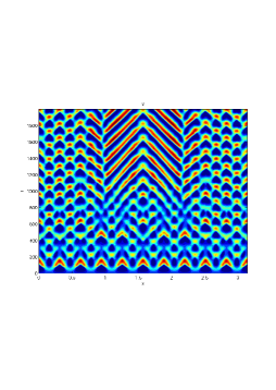
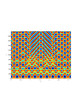
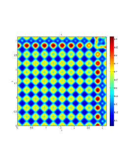
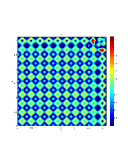
In our numerical simulation both in the one-dimensional and two-dimensional case, with specific parameter set as show in figure (3)-figure (7), different types of dynamics are observed as a result of the value of the Allee threshold mm.
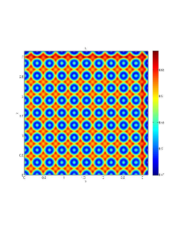
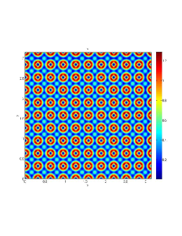
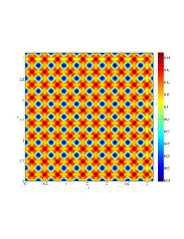
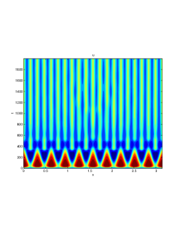
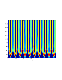
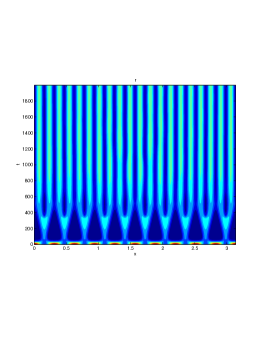
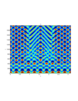
From figure (3)-figure (4), we numerically observe that change in mm can result in disappearance of patterns or the appearance of patterns. Specifically from figure (3)-figure (4), patterns where observed when m=0.01m=0.01 but these patterns change as mm gets larger and finally at m=0.5m=0.5, these patterns completely disappear. The critical Allee threshold mm, for patterns to disappear, depends on the parameter set being used. In some cases, patterns where observed when m=0m=0 but as m0.2m\to 0.2 and beyond, these patterns disappeared.
Refer to caption
Refer to caption
Refer to caption
Figure 3: The densities of the three species are shown as contour plots in the x-t plane (1 dimensional in space). The long-time simulation yields stripes-spots mixture pattern, that are spatio-temporal. The parameters are: m=0.01,w1=0.96,w2=0.52,w3=1.06,w4=0.37,a2=0.014,D3=0.1,c=0.1,d1=103,d2=105,d3=105m=0.01,w_{1}=0.96,w_{2}=0.52,w_{3}=1.06,w_{4}=0.37,a_{2}=0.014,D_{3}=0.1,c=0.1,d_{1}=10^{-3},d_{2}=10^{-5},d_{3}=10^{-5}.
Refer to caption
Refer to caption
Refer to caption
Figure 4: The densities of the three species are shown as contour plots in the x-y plane (2 dimensional in space). The long-time simulation yields spots pattern. The parameters are: m=0.01,w1=0.96,w2=0.52,w3=1.06,w4=0.37,a2=0.014,D3=0.1,c=0.1,d1=103,d2=105,d3=105m=0.01,w_{1}=0.96,w_{2}=0.52,w_{3}=1.06,w_{4}=0.37,a_{2}=0.014,D_{3}=0.1,c=0.1,d_{1}=10^{-3},d_{2}=10^{-5},d_{3}=10^{-5}.

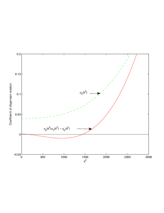
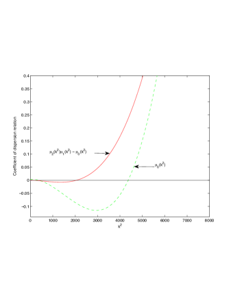
It is also conclusive from figure (5)-figure (7) that Allee threshold has an effect on the type of patterns that do form particularly, as in the case of figure (5) and (7), changing mm, can change spatio-temporal patterns to a fixed spatial patterns. This behavior can be observed using the dispersion relation as shown in figure (9). In choosing μ0(k2)<0\mu_{0}(k^{2})<0 for some kk, which will mostly result in fixed spatial patterns, changing the value of mm does not result in a change in the type of patterns formed, but parameters move out of the Turing space. Therefore in our numerical experiments we do not find parameters such that fixed spatial patterns can change to spatial-temporal patterns, as mm increases from zero.

Refer to caption
Refer to caption
Refer to caption
Figure 5: The densities of the three species are shown as contour plots in the x-t plane (1 dimensional in space). The long-time simulation yields spot and arrow type patterns. The parameters are: m=0,w1=0.95,w2=0.3,w3=0.82,w4=0.53,a2=0.01,D3=0.1,c=0.1,d1=103,d2=105,d3=105m=0,w_{1}=0.95,w_{2}=0.3,w_{3}=0.82,w_{4}=0.53,a_{2}=0.01,D_{3}=0.1,c=0.1,d_{1}=10^{-3},d_{2}=10^{-5},d_{3}=10^{-5}
Refer to caption
Refer to caption
Refer to caption
Figure 6: The densities of the three species are shown as contour plots in the x-y plane (2 dimensional in space). The long-time simulation yields spot patterns. The parameters are: m=0,w1=0.95,w2=0.3,w3=0.82,w4=0.53,a2=0.01,D3=0.1,c=0.1,d1=103,d2=105,d3=105m=0,w_{1}=0.95,w_{2}=0.3,w_{3}=0.82,w_{4}=0.53,a_{2}=0.01,D_{3}=0.1,c=0.1,d_{1}=10^{-3},d_{2}=10^{-5},d_{3}=10^{-5}
Refer to caption
Refer to caption
Refer to caption
Figure 7: The densities of the three species are shown as contour plots in the x-t plane (1 dimensional in space). The long-time simulation yields strip patterns. The parameters are: m=0.1,w1=0.95,w2=0.3,w3=0.82,w4=0.53,a2=0.01,D3=0.1,c=0.1,d1=103,d2=105,d3=105m=0.1,w_{1}=0.95,w_{2}=0.3,w_{3}=0.82,w_{4}=0.53,a_{2}=0.01,D_{3}=0.1,c=0.1,d_{1}=10^{-3},d_{2}=10^{-5},d_{3}=10^{-5}
Refer to caption
Refer to caption
Refer to caption
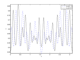
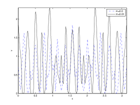
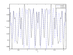
Figure 8: The density of the three species shown in figure 3 has m=0.01m=0.01. We want to compare this density to the case where m=0m=0. Thus we run a simulation with m=0m=0, and the same parameters in figure 3, w1=0.95,w2=0.3,w3=0.82,w4=0.53,a2=0.01,D3=0.1,c=0.1,d1=103,d2=105,d3=105.w_{1}=0.95,w_{2}=0.3,w_{3}=0.82,w_{4}=0.53,a_{2}=0.01,D_{3}=0.1,c=0.1,d_{1}=10^{-3},d_{2}=10^{-5},d_{3}=10^{-5}.

We next observe the densities at time t=1500 for m=0m=0 (dashed line) vs m=0.01m=0.01 (solid line), to see how the species density changes in space as the Allee threshold mm changes.

Refer to caption
Refer to caption
Figure 9: Plot of coefficient of dispersion relation with m=0m=0 and m=0.1m=0.1 for figure (5) and figure (6) respectively.

Table (2), also displays the fact that no patterns were observed as mm increases from m=0.01m=0.01 to m=0.5m=0.5 from figure (3) and figure (4) because mm can destabilizes an already stable equilibrium point in the ode model as in when k=0k=0. Hence as in figure (3) and figure (4) where m=0.01m=0.01 produces patterns since E8(u,v,r)E_{8}(u^{*},v^{*},r^{*}) is stable when k=0k=0, this stable (++) equilibrium point becomes unstable (-) even when k=0k=0.

mm HH=μ0(k2=0)H_{H}=\mu_{0}(k^{2}=0) HH=[μ2μ1μ0](k2=0)H_{H}=[\mu_{2}\mu_{1}-\mu_{0}](k^{2}=0) Pattern
0 ++ ++ Patterns may occur
0.10.1 ++ ++ Patterns may occur
0.20.2 - - No Patterns
0.30.3 - - No Patterns
0.40.4 - - No Patterns
0.50.5 - - No Patterns
Table 2: The influence of mm on the sign of 𝝁𝟎(k2)\boldsymbol{\mu_{0}}(k^{2}) and [𝝁𝟐𝝁𝟏𝝁𝟎](k2)[\boldsymbol{\mu_{2}}\boldsymbol{\mu_{1}}-\boldsymbol{\mu_{0}}](k^{2}). Describing the stability of E8(u,v,r)E_{8}(u^{*},v^{*},r^{*}) when k=0k=0 and how its might lead to pattern formation. The parameters are: w1=0.96,w2=0.52,w3=1.06,w4=0.37,a2=0.014,D3=0.1,c=0.1,d1=103,d2=105,d3=105w_{1}=0.96,w_{2}=0.52,w_{3}=1.06,w_{4}=0.37,a_{2}=0.014,D_{3}=0.1,c=0.1,d_{1}=10^{-3},d_{2}=10^{-5},d_{3}=10^{-5}.

6 Discussion

In this manuscript we have considered a spatially explicit ratio dependent three species food chain model, with a strong Allee effect in the top predator. The model represents dynamics of three interacting species in “well-mixed” conditions and is applicable to ecological problems in terrestrial, as well as aquatic systems. Our goal is to understand the effect of the Allee threshold on the system dynamics, as there is not much work on Allee effects in multi-trophic level food chains, and we hope to address this here.

We first prove the existence of a global attractor for the model. In many systems an interesting question is to consider the effect on the global attractor, under perturbation of the physical parameters in the system. Most often continuity cannot be proven, but upper semi-continuity can. We show that the global attractor is upper semi-continuous w.r.t the Allee threshold parameter mm, that is distE(𝒜m,𝒜0)0,asm0+dist_{E}(\mathcal{A}_{m},\mathcal{A}_{0})\rightarrow 0,\ \mbox{as}\ m\rightarrow 0^{+}, via theorem 3.3. To the best of our knowledge this is the first robustness result for a three-species model with strong Allee effect. Unless a systems dynamics are robust, there is no possibility to capture the same ecological behavior in a laboratory experiment, or natural setting.

The next question of interest, after one has proved such a result, is estimating the rate of decay, in terms of the physical parameter in question. Since there are no theoretical results to estimate the decay rate to the target attractor (that is when m=0m=0), we choose to investigate this rate numerically. We find decay estimates of the order of 𝒪(mγ)\mathcal{O}(m^{\gamma}), where γ\gamma is found explicitly to be slightly less, but very close to 1.

We also find that mm effects the spatiotemporal dynamics of the system in two distinct ways.
(1) It changes the Turing patterns that occur in the system, in both one and two spatial dimensions. That is varying mm, has a distinct effect on the sorts of Turing patterns that form. This can have interesting effects on the patchiness of spatially dispersing species. Our results say that if one can effect the Allee threshold in the top predator, one can effectively change the spatial concentrations of the species involved. This is best visualized in figure 8. This could have many potential applications in Allee mediated biological control, and conservation, as recently biologists have begun to consider Allee effects as beneficial in limiting establishment of an invading species [28].
(2) It facilitates overexploitation phenomenon. That is without mm, or when m=0m=0, one does not see extinction in top predator, as the origin becomes unstable. However, introducing it stabilises the origin, and low initial concentrations of rr, may yield extinction, via theorems 4.1. This has many possible applications to top down trophic cascades and cascade control. This also tells us that in a three species system, where the top predator can switch its food source, only having an Allee effect in place can possibly drive it to extinction, thus bring about true overexploitation. This could have potential applications in Allee mediated biological control, if the top predator is an invasive species.

As future investigations it would be interesting to try to model weak Allee effects in top predator, and/or Allee effects in the other species as well, be they weak or strong. It has been stipulated with evidence, that two or more Allee effects can occur simultaneously in the same population[4]. Thus an extremely interesting question would be to consider different type of Allee effects in the different species, and investigate the interplay of the various Allee thresholds, as they affect the dynamics of the system. All in all our results would be of interest to both the mathematical and ecological communities, and in particular to groups that are interested in conservation efforts in food chain systems, cascade control, such as in many aquatic systems, and even Allee mediated biological control.

References

  • [1] Peter A Abrams and Lev R Ginzburg. The nature of predation: prey dependent, ratio dependent or neither? Trends in Ecology & Evolution, 15(8):337–341, 2000.
  • [2] Warder Clyde Allee. Co-operation among animals. American Journal of Sociology, pages 386–398, 1931.
  • [3] Warder Clyde Allee, Orlando Park, Alfred Edwards Emerson, Thomas Park, Karl P Schmidt, et al. Principles of animal ecology. Number Edn 1. WB Saundere Co. Ltd., 1949.
  • [4] Luděk Berec, Elena Angulo, and Franck Courchamp. Multiple allee effects and population management. Trends in Ecology & Evolution, 22(4):185–191, 2007.
  • [5] Mathematical Bioeconomics. The optimal management of renewable resources, 1990.
  • [6] Stephen R Carpenter, James F Kitchell, and James R Hodgson. Cascading trophic interactions and lake productivity. BioScience, pages 634–639, 1985.
  • [7] Colin W Clark. The worldwide crisis in fisheries: economic models and human behavior. Cambridge University Press, 2006.
  • [8] JM Drake and AM Kramer. Allee effects. Nat. Educ. Knowl, 3(10):2, 2011.
  • [9] David Gottlieb and Liviu Lustman. The spectrum of the chebyshev collocation operator for the heat equation. SIAM journal on numerical analysis, 20(5):909–921, 1983.
  • [10] Dan Henry. Geometric theory of semilinear parabolic equations, volume 840. Springer-Verlag New York, 1981.
  • [11] Jan S Hesthaven, Sigal Gottlieb, and David Gottlieb. Spectral methods for time-dependent problems, volume 21. Cambridge University Press, 2007.
  • [12] Yang Kuang and Edoardo Beretta. Global qualitative analysis of a ratio-dependent predator–prey system. Journal of Mathematical Biology, 36(4):389–406, 1998.
  • [13] Martin Liermann and Ray Hilborn. Depensation: evidence, models and implications. Fish and Fisheries, 2(1):33–58, 2001.
  • [14] Andrew Morozov, Sergei Petrovskii, and Bai-Lian Li. Bifurcations and chaos in a predator-prey system with the allee effect. Proceedings of the Royal Society of London. Series B: Biological Sciences, 271(1546):1407–1414, 2004.
  • [15] James D Murray. Mathematical biology i: An introduction, vol. 17 of interdisciplinary applied mathematics, 2002.
  • [16] Akira Okubo and Smon A Levin. Diffusion and ecological problems: modern perspectives, volume 14. Springer Science & Business Media, 2013.
  • [17] Pallav Jyoti Pal and Prashanta Kumar Mandal. Bifurcation analysis of a modified leslie–gower predator–prey model with beddington–deangelis functional response and strong allee effect. Mathematics and Computers in Simulation, 97:123–146, 2014.
  • [18] Rana D Parshad, Hamid Ait Abderrahmane, Ranjit Kumar Upadhyay, and Nitu Kumari. Finite time blowup in a realistic food-chain model. ISRN Biomathematics, 2013, 2013.
  • [19] Rana D Parshad, Nitu Kumari, Aslan R Kasimov, and Hamid Ait Abderrahmane. Turing patterns and long-time behavior in a three-species food-chain model. Mathematical biosciences, 254:83–102, 2014.
  • [20] Rana D Parshad and Ranjit K Upadhyay. Investigation of long time dynamics of a diffusive three species aquatic model. Dynamics of Partial Differential Equations, 7(3):217–244, 2010.
  • [21] Sergei V Petrovskii, Andrew Y Morozov, and Ezio Venturino. Allee effect makes possible patchy invasion in a predator–prey system. Ecology Letters, 5(3):345–352, 2002.
  • [22] George R Sell and Yuncheng You. Dynamics of evolutionary equations, volume 143. Springer Science & Business Media, 2013.
  • [23] Moitri Sen, Malay Banerjee, and Andrew Morozov. Bifurcation analysis of a ratio-dependent prey–predator model with the allee effect. Ecological Complexity, 11:12–27, 2012.
  • [24] Swarnali Sharma and GP Samanta. A ratio-dependent predator-prey model with allee effect and disease in prey. Journal of Applied Mathematics and Computing, 47(1-2):345–364, 2014.
  • [25] Joel Smoller. Shock waves and reaction?diffusion equations, volume 258. Springer Science & Business Media, 1994.
  • [26] Philip A Stephens and William J Sutherland. Consequences of the allee effect for behaviour, ecology and conservation. Trends in Ecology & Evolution, 14(10):401–405, 1999.
  • [27] Roger Temam. Infinite-dimensional dynamical systems in mechanics and physics, volume 68. Springer Science & Business Media, 2012.
  • [28] Patrick C Tobin, Luděk Berec, and Andrew M Liebhold. Exploiting allee effects for managing biological invasions. Ecology letters, 14(6):615–624, 2011.
  • [29] Alan Mathison Turing. The chemical basis of morphogenesis. Philosophical Transactions of the Royal Society of London B: Biological Sciences, 237(641):37–72, 1952.
  • [30] Ranjit Kumar Upadhyay and Vikas Rai. Why chaos is rarely observed in natural populations. Chaos, Solitons & Fractals, 8(12):1933–1939, 1997.
  • [31] George AK Van Voorn, Lia Hemerik, Martin P Boer, and Bob W Kooi. Heteroclinic orbits indicate overexploitation in predator–prey systems with a strong allee effect. Mathematical biosciences, 209(2):451–469, 2007.
  • [32] Jinfeng Wang, Junping Shi, and Junjie Wei. Dynamics and pattern formation in a diffusive predator–prey system with strong allee effect in prey. Journal of Differential Equations, 251(4):1276–1304, 2011.
  • [33] KAJ White and CA Gilligan. Spatial heterogeneity in three species, plant–parasite–hyperparasite, systems. Philosophical Transactions of the Royal Society B: Biological Sciences, 353(1368):543–557, 1998.

7 Appendix

7.1 Nondimensionalisation

The model system in (2)-(4) is a nondimensionalised version of the following system

UT\displaystyle{\partial U\over{\partial T}} =DUΔU+A1UB1U2W1UVβ1V+U,\displaystyle=D_{U}\Delta U+A_{1}U-B_{1}U^{2}-\frac{W_{1}UV}{\beta_{1}V+U}, (73a)
VT\displaystyle{\partial V\over{\partial T}} =DVΔVA2V+W2UVβ1V+UW3VRβ3R+V,\displaystyle=D_{V}\Delta V-A_{2}V+\frac{W_{2}UV}{\beta_{1}V+U}-\frac{W_{3}VR}{\beta_{3}R+V}, (73b)
RT\displaystyle{\partial R\over{\partial T}} =DRΔR+R(RM)(CW4RV+A3).\displaystyle=D_{R}\Delta R+R\big{(}{{R-M}}\big{)}\bigg{(}C-\frac{W_{4}R}{V+A_{3}}\bigg{)}. (73c)

A1A_{1} is the self-growth rate of the prey population UU. A2A_{2} the intrinsic death rate of the specialist predator VV in the absence of its only food UU, CC measures the rate of self-reproduction of the generalist predator RR. B1B_{1} measures the strength of competition among individuals of the prey species UU. WisW_{i}^{\prime}s are the maximum values which per capita growth rate can attain. A3A_{3} represents the residual loss in RR population due to severe scarcity of its favorite food VV. β1\beta_{1} is the parameters that describes the handling time of the prey UU by predator VV, and β3\beta_{3} is the parameter that describes the handling time of the prey VV by predator RR.

We will now go over the details of the nondimensionalisation. We consider (73), and aim to introduce a change of variables and time scaling which reduces the number of parameters of model system (73)‎. We take

u\displaystyle u =UB1A1,v=VB1β1A1,r=Rb1β1β3A1,\displaystyle={UB_{1}\over A_{1}},\quad v={VB_{1}\beta_{1}\over A_{1}},\quad r={Rb_{1}\beta_{1}\beta_{3}\over A_{1}},
t\displaystyle t =TA1,w1=W1β1A1,a2=A2A1,\displaystyle={T\over{A_{1}}},\quad w_{1}={W_{1}\over\beta_{1}A_{1}},\quad a_{2}={A_{2}\over A_{1}},
w2\displaystyle w_{2} =W2A1,w3=W3β3A1,c=CA1A1B1β1β3,\displaystyle={W_{2}\over A_{1}},\quad w_{3}={W_{3}\over\beta_{3}A_{1}},\quad c={CA_{1}\over{A_{1}B_{1}\beta_{1}\beta_{3}}},
m\displaystyle m =MB1β1β3A1,D3=A3B1β1A1,w4=W4B1B12β1β32,\displaystyle={MB_{1}\beta_{1}\beta_{3}\over A_{1}},\quad D_{3}={A_{3}B_{1}\beta_{1}\over A_{1}},\quad w_{4}={W_{4}B_{1}\over{B_{1}^{2}\beta_{1}\beta_{3}^{2}}},
d1\displaystyle d_{1} =DUπ2B1L2,d2=DVπ2B1β1L2,d3=DRπ2B1β1β3L2.\displaystyle={D_{U}\pi^{2}\over B_{1}L^{2}},\quad d_{2}={D_{V}\pi^{2}\over B_{1}\beta_{1}L^{2}},\quad d_{3}={D_{R}\pi^{2}\over{B_{1}\beta_{1}\beta_{3}L^{2}}}.

Considering Neuman boundary conditions, model system (73) reduces to

ut=d1Δu+uu2w1uvu+v,\displaystyle\frac{\partial u}{\partial t}=d_{1}\Delta u+u-u^{2}-w_{1}\frac{uv}{u+v}, (74)
vt=d2Δva2v+w2uvu+vw3(vrv+r),\displaystyle\frac{\partial v}{\partial t}=d_{2}\Delta v-a_{2}v+w_{2}\frac{uv}{u+v}-w_{3}\left(\frac{vr}{v+r}\right), (75)
rt=d3Δr+r(rm)(cw4rv+D3).\displaystyle\frac{\partial r}{\partial t}=d_{3}\Delta r+r\big{(}{{r-m}}\big{)}\bigg{(}c-\frac{w_{4}r}{v+D_{3}}\bigg{)}. (76)

Also all parameters associated with model system (74-76) are assumed to be positive constants and have the usual biological meaning.

7.2 Global existence

Here we prove proposition 2.2. The positivity of solutions follow trivially from the form of the reaction terms, which are quasi positive. By the positivity of the first component u(t,.)u(t,.) of the solution to (2) on [0,Tmax)[0,T_{\max}) ×Ω\times\Omega, we get from equation (2)

utd1Δua1u, on [0,Tmax)×Ω,\frac{\partial u}{\partial t}-d_{1}\Delta u\leq a_{1}u,\text{ \ on }[0,T_{\max})\times\Omega, (77)

then we use a comparison argument [25]. That is, we can compare the solution uu of (77) to the solution uu^{*}, of the linear heat equation

utd1Δu=a1u, on [0,Tmax)×Ω,\frac{\partial u^{*}}{\partial t}-d_{1}\Delta u^{*}=a_{1}u^{*},\text{ \ on }[0,T_{\max})\times\Omega, (78)

where uu^{*} satisfies the same initial and boundary conditions as uu. Clearly uuu\leq u^{*}, and since uu^{*} (being the solution of a linear heat equation) is bounded, so is uu, and we deduce

u(t,.)C1,u(t,.)\leq C_{1}, (79)

where C1C_{1} is a constant depending only on TmaxT_{\max}. Then equation (3) gives

vtd2Δvw1C1v, on [0,Tmax)×Ω,\frac{\partial v}{\partial t}-d_{2}\Delta v\leq w_{1}C_{1}v,\text{ \ on }[0,T_{\max})\times\Omega, (80)

which implies by the same arguments

v(t,.)C2, on [0,Tmax)×Ω,v(t,.)\leq C_{2},\text{ \ on }[0,T_{\max})\times\Omega, (81)

where C2C_{2} is a constant depending only on TmaxT_{\max}. To get a bound on the component rr we apply Young’s inequality to yield

rtd3Δr+Mcr\displaystyle\frac{\partial r}{\partial t}-d_{3}\Delta r+Mcr
=(c+Mw3v+D3)r2(w3v+D3)r3\displaystyle=\left(c+\frac{Mw_{3}}{v+D_{3}}\right)r^{2}-\left(\frac{w_{3}}{v+D_{3}}\right)r^{3}
(c+Mw3D3)r2(w3v+D3)r3\displaystyle\leq\left(c+\frac{Mw_{3}}{D_{3}}\right)r^{2}-\left(\frac{w_{3}}{v+D_{3}}\right)r^{3}
=(c+Mw3D3)(v+D3w3)23(v+D3w3)23r2(w3v+D3)r3\displaystyle=\left(c+\frac{Mw_{3}}{D_{3}}\right)\left(\frac{v+D_{3}}{w_{3}}\right)^{\frac{2}{3}}\left(\frac{v+D_{3}}{w_{3}}\right)^{-\frac{2}{3}}r^{2}-\left(\frac{w_{3}}{v+D_{3}}\right)r^{3}
(c+Mw3D3)3(v+D3w3)2+(w3v+D3)r3(w3v+D3)r3\displaystyle\leq\left(c+\frac{Mw_{3}}{D_{3}}\right)^{3}\left(\frac{v+D_{3}}{w_{3}}\right)^{2}+\left(\frac{w_{3}}{v+D_{3}}\right)r^{3}-\left(\frac{w_{3}}{v+D_{3}}\right)r^{3}
(c+Mw3D3)3(C2+D3w3)2\displaystyle\leq\left(c+\frac{Mw_{3}}{D_{3}}\right)^{3}\left(\frac{C_{2}+D_{3}}{w_{3}}\right)^{2} (82)

Here we use the bound on vv via (81). Thus there exists a positive constant C3C_{3} such that

r(t,.)C3=(c+Mw3D3)3(C2+D3w3)2, on [0,Tmax)×Ω.r(t,.)\leq C_{3}=\left(c+\frac{Mw_{3}}{D_{3}}\right)^{3}\left(\frac{C_{2}+D_{3}}{w_{3}}\right)^{2},\text{ \ on }[0,T_{\max})\times\Omega. (83)

At this step via (79), (81), (83) standard theory [10] is applicable and the solution is global (Tmax=+T_{\max}=+\infty). This proves the proposition.

7.3 Apriori estimates

In all estimates made hence forth the constants C,C1,C2,C3,CC,C_{1},C_{2},C_{3},C_{\infty} are generic constants, that can change in value from line to line, and sometimes within the same line if so required. We estimate the gradient of rr by multiplying (4) by Δr-\Delta r, and integrating by parts and using standard methods to obtain

12ddtr22+d3Δr22=Ωr(rm)(cw4rv+D3)(Δr)𝑑x.\frac{1}{2}\frac{d}{dt}||\nabla r||^{2}_{2}+d_{3}||\Delta r||^{2}_{2}=\int_{\Omega}r(r-m)(c-w_{4}\frac{r}{v+D_{3}})(-\Delta r)dx. (84)

We have to estimate Ωr(rm)(cw4rv+D3)(Δr)𝑑x\int_{\Omega}r(r-m)(c-w_{4}\frac{r}{v+D_{3}})(-\Delta r)dx. Note

Ωr(rm)(crv+D3)(Δr)𝑑x\displaystyle\int_{\Omega}r(r-m)(c-\frac{r}{v+D_{3}})(-\Delta r)dx =Ω((c+mw4v+D3)r2w4v+D3r3mcr)(Δr)𝑑x,\displaystyle=\int_{\Omega}\left(\left(c+\frac{mw_{4}}{v+D_{3}}\right)r^{2}-\frac{w_{4}}{v+D_{3}}r^{3}-mcr\right)(-\Delta r)dx,
=Ω((c+mw4v+D3)r2w4v+D3r3)(Δr)𝑑xcmr22.\displaystyle=\int_{\Omega}\left(\left(c+\frac{mw_{4}}{v+D_{3}}\right)r^{2}-\frac{w_{4}}{v+D_{3}}r^{3}\right)(-\Delta r)dx-cm||\nabla r||^{2}_{2}.

Thus we obtain

12ddtr22+d3Δr22+cmr22=Ω((c+mw4v+D3)r2w4v+D3r3)(Δr)𝑑x.\frac{1}{2}\frac{d}{dt}||\nabla r||^{2}_{2}+d_{3}||\Delta r||^{2}_{2}+cm||\nabla r||^{2}_{2}=\int_{\Omega}\left(\left(c+\frac{mw_{4}}{v+D_{3}}\right)r^{2}-\frac{w_{4}}{v+D_{3}}r^{3}\right)(-\Delta r)dx. (85)

We now proceed in 2 steps. We first assume ((c+mw4v+D3)r2w4v+D3r3)0\left(\left(c+\frac{mw_{4}}{v+D_{3}}\right)r^{2}-\frac{w_{4}}{v+D_{3}}r^{3}\right)\geq 0.

Young’s Inequality with epsilon then gives us the following estimate

((c+mw4v+D3)r2w4v+D3r3)\displaystyle\left(\left(c+\frac{mw_{4}}{v+D_{3}}\right)r^{2}-\frac{w_{4}}{v+D_{3}}r^{3}\right) (v+D3w4)13(c+mw4v+D3)r(w4v+D3)13rw4r3v+D3,\displaystyle\leq\left(\frac{v+D_{3}}{w_{4}}\right)^{\frac{1}{3}}\left(c+\frac{mw_{4}}{v+D_{3}}\right)r\left(\frac{w_{4}}{v+D_{3}}\right)^{\frac{1}{3}}r-w_{4}\frac{r^{3}}{v+D_{3}},
(v+D3w4)49(c+mw4v+D3)43r43+w4r3v+D3w4r3v+D3,\displaystyle\leq\left(\frac{v+D_{3}}{w_{4}}\right)^{\frac{4}{9}}\left(c+\frac{mw_{4}}{v+D_{3}}\right)^{\frac{4}{3}}r^{\frac{4}{3}}+w_{4}\frac{r^{3}}{v+D_{3}}-w_{4}\frac{r^{3}}{v+D_{3}},
(v+D3w4)(c+mw4v+D3)43r43+w4r3v+D3w4r3v+D3,\displaystyle\leq\left(\frac{||v+D_{3}||_{\infty}}{w_{4}}\right)\left(c+\frac{mw_{4}}{v+D_{3}}\right)^{\frac{4}{3}}r^{\frac{4}{3}}+w_{4}\frac{r^{3}}{v+D_{3}}-w_{4}\frac{r^{3}}{v+D_{3}},
(C+D3w4)(c+mw4D3)43r43+w4r3v+D3w4r3v+D3,\displaystyle\leq\left(\frac{C+D_{3}}{w_{4}}\right)\left(c+\frac{mw_{4}}{D_{3}}\right)^{\frac{4}{3}}r^{\frac{4}{3}}+w_{4}\frac{r^{3}}{v+D_{3}}-w_{4}\frac{r^{3}}{v+D_{3}},
=(C+D3w4)(c+mw4D3)43r43.\displaystyle=\left(\frac{C+D_{3}}{w_{4}}\right)\left(c+\frac{mw_{4}}{D_{3}}\right)^{\frac{4}{3}}r^{\frac{4}{3}}.

Then we obtain

12ddtr22+d3Δr22+2cmr22\displaystyle\frac{1}{2}\frac{d}{dt}||\nabla r||^{2}_{2}+d_{3}||\Delta r||^{2}_{2}+2cm||\nabla r||^{2}_{2} =\displaystyle= Ω((c+mw4v+D3)r2w4v+D3r3)(Δr)𝑑x,\displaystyle\int_{\Omega}\left(\left(c+\frac{mw_{4}}{v+D_{3}}\right)r^{2}-\frac{w_{4}}{v+D_{3}}r^{3}\right)(-\Delta r)dx,
\displaystyle\leq (C+D3w4)(c+mw4D3)43Ωr43|Δr|𝑑x\displaystyle\left(\frac{C+D_{3}}{w_{4}}\right)\left(c+\frac{mw_{4}}{D_{3}}\right)^{\frac{4}{3}}\int_{\Omega}r^{\frac{4}{3}}|-\Delta r|dx

This follows via (7.3). Thus we obtain

12ddtr22+d3Δr22C1r8383+d32Δr22.\frac{1}{2}\frac{d}{dt}||\nabla r||^{2}_{2}+d_{3}||\Delta r||^{2}_{2}\leq C_{1}||r||^{\frac{8}{3}}_{\frac{8}{3}}+\frac{d_{3}}{2}||\Delta r||^{2}_{2}. (88)

Here C1=(C+D3w4)(c+w4D3)43C_{1}=\left(\frac{C+D_{3}}{w_{4}}\right)\left(c+\frac{w_{4}}{D_{3}}\right)^{\frac{4}{3}}. Now we can use the sobolev embedding of H1(Ω)L83(Ω)H^{1}(\Omega)\hookrightarrow L^{\frac{8}{3}}(\Omega), where C3C_{3} is the embedding constant, to obtain

ddtr22+d3Δr22C3C1(r22)(r22).\frac{d}{dt}||\nabla r||^{2}_{2}+d_{3}||\Delta r||^{2}_{2}\leq C_{3}C_{1}\left(||\nabla r||^{2}_{2}\right)\left(||\nabla r||^{2}_{2}\right). (89)

Thus

ddtr22C3C1(r22)(r22).\frac{d}{dt}||\nabla r||^{2}_{2}\leq C_{3}C_{1}(||\nabla r||^{2}_{2})(||\nabla r||^{2}_{2}). (90)

Now we invoke the estimate via (15), and the uniform Gronwall lemma to obtain

lim suptr22C.\mathop{\limsup}_{t\rightarrow\infty}||\nabla r||^{2}_{2}\leq C. (91)

Now assume ((c+mw4v+D3)r2w4v+D3r3)<0\left(\left(c+\frac{mw_{4}}{v+D_{3}}\right)r^{2}-\frac{w_{4}}{v+D_{3}}r^{3}\right)<0. Then we obtain

12ddtr22+d3Δr22+cmr22,\displaystyle\frac{1}{2}\frac{d}{dt}||\nabla r||^{2}_{2}+d_{3}||\Delta r||^{2}_{2}+cm||\nabla r||^{2}_{2},
\displaystyle\leq Ω(c+mw4D3)r2(Δr)𝑑x,\displaystyle\int_{\Omega}\left(c+\frac{mw_{4}}{D_{3}}\right)r^{2}(-\Delta r)dx,
\displaystyle\leq 2d3(c+mw4D3)r44+d32Δr22.\displaystyle\frac{2}{d_{3}}\left(c+\frac{mw_{4}}{D_{3}}\right)||r||^{4}_{4}+\frac{d_{3}}{2}||\Delta r||^{2}_{2}.

We now use the Sobolev embedding of H1(Ω)L4(Ω)H^{1}(\Omega)\hookrightarrow L^{4}(\Omega) to obtain

ddtr22+d3Δr22+cmr222d3(c+w4D3)r24,\frac{d}{dt}||\nabla r||^{2}_{2}+d_{3}||\Delta r||^{2}_{2}+cm||\nabla r||^{2}_{2}\leq\frac{2}{d_{3}}\left(c+\frac{w_{4}}{D_{3}}\right)||\nabla r||^{4}_{2}, (93)

dropping the cmr22cm||\nabla r||^{2}_{2} term yields

ddtr222d3(c+w4D3)(r22)(r22),\frac{d}{dt}||\nabla r||^{2}_{2}\leq\frac{2}{d_{3}}\left(c+\frac{w_{4}}{D_{3}}\right)\left(||\nabla r||^{2}_{2}\right)\left(||\nabla r||^{2}_{2}\right), (94)
lim suptr22C,\mathop{\limsup}_{t\rightarrow\infty}||\nabla r||^{2}_{2}\leq C, (95)

7.4 Apriori estimates independent of the parameter mm

Recall the following L2L^{2} estimate

12ddtr22+d3r22+cmr22+Ωw4v+D3r4𝑑xΩ(c+mw4v+D3)r3𝑑x.\frac{1}{2}\frac{d}{dt}||r||^{2}_{2}+d_{3}||\nabla r||^{2}_{2}+cm||r||^{2}_{2}+\int_{\Omega}\frac{w_{4}}{v+D_{3}}r^{4}dx\leq\int_{\Omega}\left(c+\frac{mw_{4}}{v+D_{3}}\right)r^{3}dx.

We then use Hölder’s inequality followed by Young’s inequality to obtain

12ddtr22+d3r22+cmr22+Ωw4v+D3r4𝑑x,\displaystyle\frac{1}{2}\frac{d}{dt}||r||^{2}_{2}+d_{3}||\nabla r||^{2}_{2}+cm||r||^{2}_{2}+\int_{\Omega}\frac{w_{4}}{v+D_{3}}r^{4}dx,
34Ωw4v+D3r4𝑑x+|Ω|14(c+w4D3)(w4D3)14.\displaystyle\leq\frac{3}{4}\int_{\Omega}\frac{w_{4}}{v+D_{3}}r^{4}dx+|\Omega|^{\frac{1}{4}}\left(c+\frac{w_{4}}{D_{3}}\right)\left(\frac{w_{4}}{D_{3}}\right)^{\frac{1}{4}}.

Now we drop the cmr22cm||r||^{2}_{2} term from the left hand side, to avoid the singularity caused by 1m\frac{1}{m}, the d3r22d_{3}||\nabla r||^{2}_{2}, and use the estimate on v||v||_{\infty} via (27), and the embedding of L4(Ω)L2(Ω)L^{4}(\Omega)\hookrightarrow L^{2}(\Omega) to obtain

ddtr22+Cw4C+D3r222|Ω|14(c+w4D3)(w4D3)14.\frac{d}{dt}||r||^{2}_{2}+\frac{Cw_{4}}{C+D_{3}}||r||^{2}_{2}\leq 2|\Omega|^{\frac{1}{4}}\left(c+\frac{w_{4}}{D_{3}}\right)\left(\frac{w_{4}}{D_{3}}\right)^{\frac{1}{4}}. (97)

Here, we assume r21||r||_{2}\geq 1, else we already have a bound for r2||r||_{2}. Next we use Gronwall’s inequality to obtain

r22e(Cw4C+D3)tr022+2|Ω|14(c+w4D3)(w4D3.)14(C+D3)Cw4.||r||^{2}_{2}\leq e^{-\left(\frac{Cw_{4}}{C+D_{3}}\right)t}||r_{0}||^{2}_{2}+\frac{2|\Omega|^{\frac{1}{4}}\left(c+\frac{w_{4}}{D_{3}}\right)\left(\frac{w_{4}}{D_{3}}.\right)^{\frac{1}{4}}(C+D_{3})}{Cw_{4}}. (98)

Thus for t>t0=max(t+1,ln(r022)(Cw4C+D3))t>t_{0}=\max(t^{*}+1,\frac{\ln(||r_{0}||^{2}_{2})}{\left(\frac{Cw_{4}}{C+D_{3}}\right)}), we obtain

r221+2|Ω|14(c+w4D3)(w4D3)14(C+D3)Cw4,||r||^{2}_{2}\leq 1+\frac{2|\Omega|^{\frac{1}{4}}\left(c+\frac{w_{4}}{D_{3}}\right)\left(\frac{w_{4}}{D_{3}}\right)^{\frac{1}{4}}(C+D_{3})}{Cw_{4}}, (99)

which is a uniform L2(Ω)L^{2}(\Omega) bound in rr that is independent of the Allee parameter mm, time and initial data.

We next focus on making H1(Ω)H^{1}(\Omega) estimates, that are independent of the Allee parameter mm.

We choose the estimate derived in (99) for r2||r||_{2} and insert this in (15) to obtain

tt+1r22𝑑s\displaystyle\int^{t+1}_{t}||\nabla r||^{2}_{2}ds
1+2|Ω|14(c+w4D3)(w4D3)14(C+D3)Cw4+2|Ω|14(c+w4D3)(w4D3)14,\displaystyle\leq 1+\frac{2|\Omega|^{\frac{1}{4}}\left(c+\frac{w_{4}}{D_{3}}\right)\left(\frac{w_{4}}{D_{3}}\right)^{\frac{1}{4}}(C+D_{3})}{Cw_{4}}+2|\Omega|^{\frac{1}{4}}\left(c+\frac{w_{4}}{D_{3}}\right)\left(\frac{w_{4}}{D_{3}}\right)^{\frac{1}{4}},
fort>t0.\displaystyle\ \mbox{for}\ t>t_{0}. (100)

Now we choose

Km=max(2d3(c+mw4D3),C3(C+D3w4)(c+mw4D3)43).K_{m}=\max\left(\frac{2}{d_{3}}\left(c+\frac{mw_{4}}{D_{3}}\right),C_{3}\left(\frac{C+D_{3}}{w_{4}}\right)\left(c+\frac{mw_{4}}{D_{3}}\right)^{\frac{4}{3}}\right). (101)

Then, we can majorise the right hand side of the above by plugging in m=1m=1. Since the above quantities are not singular in mm, this is possible. Thus we obtain

K=max(2d3(c+w4D3),C3(C+D3w4)(c+w4D3)43),K=\max\left(\frac{2}{d_{3}}\left(c+\frac{w_{4}}{D_{3}}\right),C_{3}\left(\frac{C+D_{3}}{w_{4}}\right)\left(c+\frac{w_{4}}{D_{3}}\right)^{\frac{4}{3}}\right), (102)

going back to the H1(Ω)H^{1}(\Omega) estimates in (91), and (95) one obtains,

ddtr22K(r22)(r22).\frac{d}{dt}||\nabla r||^{2}_{2}\leq K\left(||\nabla r||^{2}_{2}\right)\left(||\nabla r||^{2}_{2}\right). (103)

Also note the integral in time estimate via (7.4) is now independent of mm. This allows us to apply the uniform Gronwall lemma on (103) with β(t)=r22,ζ(t)=Kr22,h(t)=0,q=1\beta(t)=||\nabla r||^{2}_{2},\ \zeta(t)=K||\nabla r||^{2}_{2},\ h(t)=0,q=1, and the estimate via (7.4) to yield the following bound

r22\displaystyle||\nabla r||^{2}_{2}
CKeKCK,fort>t1=t0+1.\displaystyle\leq C_{K}e^{KC_{K}},\ \mbox{for}\ t>t_{1}=t_{0}+1. (104)

Thus the H1(Ω)H^{1}(\Omega) estimate for rr can be made independent of mm.

7.5 Upper semi-continuity of global attractors

In this section we prove upper semi continuity of global attractors. We first introduce certain concepts pertinent to the upper semicontinuity of attractors.

Definition 7.1 (Uniform dissipativity)

Suppose there is a family of semiflows {{Sλ(t)}t0}λΛ\{\{S_{\lambda}(t)\}_{t\geq 0}\}_{\lambda\in\Lambda} on a Banach space HH, where Λ\Lambda is an open set in a Euclidean space of parameter λ\lambda, is called uniformly dissipative at λ0Λ\lambda_{0}\in\Lambda, if there is a neighborhood 𝒩\mathcal{N} of λ0\lambda_{0} in Λ\Lambda and there is a bounded set H\mathcal{B}\subset H such that \mathcal{B} is an absorbing set for each semiflow Sλ(t)S_{\lambda}(t), λ𝒩\lambda\in\mathcal{N}, in common.

Definition 7.2 (Upper semicontinuity)

A family of semiflows {{Sλ(t)}t0}λΛ\{\{S_{\lambda}(t)\}_{t\geq 0}\}_{\lambda\in\Lambda} on a Banach space HH, where Λ\Lambda is an open set in a Euclidean space of parameter λ\lambda, and that there exists a global attractor 𝒜λ\mathcal{A}_{\lambda} in \mathcal{H} for each semiflow {{Sλ(t)}t0}λΛ\{\{S_{\lambda}(t)\}_{t\geq 0}\}_{\lambda\in\Lambda}. If λ0Λ\lambda_{0}\in\Lambda and

dist(𝒜λ,𝒜λ0)0,asλλ0inΛ,dist_{\mathcal{H}}(\mathcal{A}_{\lambda},\mathcal{A}_{\lambda_{0}})\rightarrow 0,\ \mbox{as}\ \lambda\rightarrow\lambda_{0}\ \mbox{in}\ \Lambda,

with respect to the Hausdorff semidistance, then we say that the family of global attractors {𝒜λ}λΛ\{\mathcal{A}_{\lambda}\}_{\lambda\in\Lambda} is upper semicontinuous at λ0\lambda_{0}, or that 𝒜λ\mathcal{A}_{\lambda} is robust at λ0\lambda_{0}.

We next recall the following lemma

Lemma 7.3 (Gronwall-Henry Inequality)

Let ψ(t)\psi(t) be a nonnegative function in Lloc[0,T;)L^{\infty}_{loc}[0,T;\mathbb{R}) and ζ(.)\zeta(.) \in Lloc1[0,T;)L^{1}_{loc}[0,T;\mathbb{R}), such that the following inequality is satisfied:

ψ(t)ζ(t)+μ0t(ts)r1ψ(s)𝑑s,t(0,T),\psi(t)\leq\zeta(t)+\mu\int^{t}_{0}(t-s)^{r-1}\psi(s)ds,\ t\in(0,T), (105)

where 0<T0<T\leq\infty, and μ,r\mu,r are positive constants. Then it holds that

ψ(t)ζ(t)+κ0tΦ(κ(ts))ψ(s)𝑑s,t(0,T),\psi(t)\leq\zeta(t)+\kappa\int^{t}_{0}\Phi(\kappa(t-s))\psi(s)ds,\ t\in(0,T), (106)

where κ=(μΓ(r))1r\kappa=(\mu\Gamma(r))^{\frac{1}{r}}, Γ(.)\Gamma(.) is the gamma function, and the function ϕ(t)\phi(t) is given by

ϕ(t)=n=1nrΓ(nr+1)tnr1=n=1nrΓ(nr)tnr1.\phi(t)=\sum^{\infty}_{n=1}\frac{nr}{\Gamma(nr+1)}t^{nr-1}=\sum^{\infty}_{n=1}\frac{nr}{\Gamma(nr)}t^{nr-1}. (107)

We state the following theorem

Theorem 7.4

Consider the reaction diffusion equation described via (2)-(4) where Ω\Omega is of spatial dimension n=1,2,3n=1,2,3. There exists a universal constant K>0K_{\infty}>0, independent of the Allee parameter mm that bounds uniformly in LL^{\infty} the family of global attractors 𝒜m\mathcal{A}_{m}. That is,

0m1𝒜mBL(0,K).\bigcup_{0\leq m\leq 1}\mathcal{A}_{m}\subset B_{L^{\infty}}(0,K_{\infty}). (108)

Where BL(0,K)B_{L^{\infty}}(0,K_{\infty}) is the closed ball of radius KK_{\infty} in the space L(Ω)L^{\infty}(\Omega), with K=3CK_{\infty}=3C, where the CC is from (27).

This follows from the estimates via (27).

We next focus on the uniform dissipativity in L2(Ω)L^{2}(\Omega). The uniform in parameter mm L2(Ω)L^{2}(\Omega) estimate via (99) enables us to state the following theorem

Theorem 7.5

Consider the reaction diffusion system described via (2)-(4) where Ω\Omega is of spatial dimension n=1,2,3n=1,2,3. The family of semiflows {{Sm(t)}t0}m0\{\{S_{m}(t)\}_{t\geq 0}\}_{m\geq 0} for this system on HH, is uniformly dissipative at m=0m=0. Specifically there exists a constant KH>0K_{H}>0 such that the ball BH(0,KH)B_{H}(0,K_{H}), which is the closed ball of radius KHK_{H} in the space HH is a common absorbing set for the semiflows {{Sm(t)}t0}\{\{S_{m}(t)\}_{t\geq 0}\} for all m[0,1]m\in[0,1]. Here KH=1+2|Ω|14(c+w4D3)(w4D3)14(C+D3)Cw4+2CK_{H}=1+\frac{2|\Omega|^{\frac{1}{4}}\left(c+\frac{w_{4}}{D_{3}}\right)\left(\frac{w_{4}}{D_{3}}\right)^{\frac{1}{4}}(C+D_{3})}{Cw_{4}}+2C, where the 2C2C comes from lemma 2.4.

Next, let us choose (u0,v0,r0)(u_{0},v_{0},r_{0}) \in 𝒰\mathcal{U}. We know 𝒰BH(0,KH)\mathcal{U}\subset B_{H}(0,K_{H}), the common absorbing ball in HH for the semiflow Sm(t)S_{m}(t), m[0,1]m\in[0,1], from theorem 7.5. We use the earlier H1(Ω)H^{1}(\Omega) and L2(Ω)L^{2}(\Omega) estimates on u,vu,v from lemma 2.4, noticing that they do not depend on mm, we also use (99) and (7.4) to obtain

Sm(t)((u0,v0,r0))E2\displaystyle||S_{m}(t)((u_{0},v_{0},r_{0}))||^{2}_{E}
=(u,v,r)2+(u,v,r)2\displaystyle=||(\nabla u,\nabla v,\nabla r)||^{2}+||(u,v,r)||^{2}
4C+CKeKCK+1+2|Ω|14(c+w4D3)(w4D3)14(C+D3)Cw4.\displaystyle\leq 4C+C_{K}e^{KC_{K}}+1+\frac{2|\Omega|^{\frac{1}{4}}\left(c+\frac{w_{4}}{D_{3}}\right)\left(\frac{w_{4}}{D_{3}}\right)^{\frac{1}{4}}(C+D_{3})}{Cw_{4}}. (109)

This is true for any (u0,v0,r0)𝒰(u_{0},v_{0},r_{0})\in\mathcal{U} and m[0,1]m\in[0,1]. Now by invariance Sm(t)𝒜m=𝒜mS_{m}(t)\mathcal{A}_{m}=\mathcal{A}_{m}, and so 𝒜mBE(0,KE)\mathcal{A}_{m}\subset B_{E}(0,K_{E}). Where

KE=4C+CKeKCK+1+2|Ω|14(c+w4D3)(w4D3)14(C+D3)Cw4.K_{E}=4C+C_{K}e^{KC_{K}}+1+\frac{2|\Omega|^{\frac{1}{4}}\left(c+\frac{w_{4}}{D_{3}}\right)\left(\frac{w_{4}}{D_{3}}\right)^{\frac{1}{4}}(C+D_{3})}{Cw_{4}}. (110)

This yields the following theorem

Theorem 7.6

Consider the reaction diffusion equation described via (2)-(4) where Ω\Omega is of spatial dimension n=1,2,3n=1,2,3. There exists a universal constant KE>0K_{E}>0, independent of the Allee parameter mm that bounds uniformly in EE the family of global attractors 𝒜m\mathcal{A}_{m}. That is,

0m1𝒜mBE(0,KE),\bigcup_{0\leq m\leq 1}\mathcal{A}_{m}\subset B_{E}(0,K_{E}), (111)

where BE(0,KE)B_{E}(0,K_{E}) is the closed ball of radius KEK_{E} explicitly given in (110).

We next show that the trajectories Sm(t)U,t0S_{m}(t)U,t\geq 0, are uniformly EE-bounded, with respect to mm. Since the estimate in (110) does not depend on mm, we can take a supremum over m[0,1]m\in[0,1] and still achieve the same bound. Thus we have the following result

Theorem 7.7

Consider the reaction diffusion equation described via (2)-(4). There exists a universal constant KE>0K_{E}>0, independent of the Allee parameter mm such that

sup0m1supt0Sm(t)(0m1𝒜m)BE(0,KE),\sup_{0\leq m\leq 1}\sup_{t\geq 0}S_{m}(t)\left(\bigcup_{0\leq m\leq 1}\mathcal{A}_{m}\right)\subset B_{E}(0,K_{E}), (112)

where, BE(0,KE)B_{E}(0,K_{E}) is the closed ball of radius KEK_{E} in the space EE.

We next set m=0m=0 in (4) and note that the corresponding estimates in lemma 2.4 hold for u,vu,v, and do not depend on the parameter mm. Thus we carry out the analysis as in (7.4) - (110) to still yield

r22CKeKCK,fort>t1+1.\displaystyle||\nabla r||^{2}_{2}\leq C_{K}e^{KC_{K}},\ \mbox{for}\ t>t_{1}+1. (113)

Where CKeKCKC_{K}e^{KC_{K}} is independent of the parameter mm. Thus we can state the following result

Theorem 7.8

Consider the reaction diffusion equation described via (2)-(4), when m=0m=0, and where Ω\Omega is of spatial dimension n=1,2,3n=1,2,3. There exists a (H,E)(H,E) global attractor 𝒜\mathcal{A} for the system. This is compact and invariant in HH, and it attracts all bounded subsets of HH in the EE metric.

The proof of the above theorem follows essentially via theorem 3.2.

Note, since (0m1𝒜m)\left(\bigcup_{0\leq m\leq 1}\mathcal{A}_{m}\right) is a bounded set in HH, we can state the following result ,

Theorem 7.9

Consider the reaction diffusion equation described via (2)-(4), with m=0m=0. The global attractor for this system 𝒜0\mathcal{A}_{0}, attracts the set (0m1𝒜m)\left(\bigcup_{0\leq m\leq 1}\mathcal{A}_{m}\right), with respect to the EE-norm. That is

limtdistE(S0(t)(0m1𝒜m),𝒜0).\lim_{t\rightarrow\infty}dist_{E}\left(S_{0}(t)\left(\bigcup_{0\leq m\leq 1}\mathcal{A}_{m}\right),\mathcal{A}_{0}\right). (114)

We now use the Gronwall-Henry lemma, to show uniform convergence in the parameter mm.

Theorem 7.10

Consider the reaction diffusion equation described via (2)-(4), and associated semi-group Sm(t)S_{m}(t). Also consider (2)-(4), when m=0m=0, that is with associated semi-group S0(t)S_{0}(t). For any given t0t\geq 0, it holds that

supg0𝒰Sm(t)g0S0(t)g0E0,asm0+.\sup_{g_{0}\in\mathcal{U}}||S_{m}(t)g_{0}-S_{0}(t)g_{0}||_{E}\rightarrow 0,\mbox{as}\ m\rightarrow 0^{+}. (115)

For any given initial data g0𝒰g_{0}\in\mathcal{U}, we note Sm(t)g0S_{m}(t)g_{0} and S0(t)g0S_{0}(t)g_{0}, are both classical solutions, hence mild solutions. Thus we denote

w(t)=Sm(t)g0S0(t)g0,t0,withw(0)=0.w(t)=S_{m}(t)g_{0}-S_{0}(t)g_{0},t\geq 0,\ \mbox{with}\ w(0)=0. (116)

Using the form of mild solutions, we can write down the following,

w(t)=0teA(tσ)[f0(Sm(σ)g0)f0(S0(σ)g0)]𝑑σ+m0teA(tσ)h(Sm(σ)g0)𝑑σ,t0.w(t)=\int^{t}_{0}e^{A(t-\sigma)}[f_{0}(S_{m}(\sigma)g_{0})-f_{0}(S_{0}(\sigma)g_{0})]d\sigma+m\int^{t}_{0}e^{A(t-\sigma)}h(S_{m}(\sigma)g_{0})d\sigma,\ t\geq 0. (117)

Here eAte^{At} , t0t\geq 0 is the C0C_{0} semi-group generated by A:D(A)HA:D(A)\rightarrow H. Note

fm(u,v,r)=(uu2w1uvu+va2v+w2uvu+vw3(vrv+r)w4v+D3r3+cr2),h(r)=(00mcr+mw4v+D3r2).f_{m}(u,v,r)=\left(\begin{array}[]{c}u-u^{2}-w_{1}\frac{uv}{u+v}\\ -a_{2}v+w_{2}\frac{uv}{u+v}-w_{3}\left(\frac{vr}{v+r}\right)\\ -\frac{w_{4}}{v+D_{3}}r^{3}+cr^{2}\\ \end{array}\ \right),h(r)=\left(\begin{array}[]{c}0\\ 0\\ -mcr+\frac{mw_{4}}{v+D_{3}}r^{2}\\ \end{array}\right). (118)

The above is easily seen to be Lipschitz continuous in EE, due to the Sobolev embedding of H1(Ω)L6(Ω)H^{1}(\Omega)\hookrightarrow L^{6}(\Omega). Here f0f_{0}, which is gotten by setting m=0m=0 in the above, is also Lipschitz continuous, thus there is a Lipschitz constant Lf0(KE)>0L_{f_{0}}(K_{E})>0, depending only on KEK_{E}, where KEK_{E} is given in (110), s.t

f0(g1)f0(g2)Lf0(KE)g1g2E,||f_{0}(g_{1})-f_{0}(g_{2})||\leq L_{f_{0}}(K_{E})||g_{1}-g_{2}||_{E}, (119)

for any g1,g2BE(0,KE)g_{1},g_{2}\in B_{E}(0,K_{E}). From theorems 7.6, 7.7 we have

w(t)E\displaystyle||w(t)||_{E}
0teA(tσ)(H,E)Lf0(KE)Sm(σ)g0S0(σ)g0E𝑑σ,\displaystyle\leq\int^{t}_{0}||e^{A(t-\sigma)}||_{\mathcal{L}(H,E)}L_{f_{0}}(K_{E})||S_{m}(\sigma)g_{0}-S_{0}(\sigma)g_{0}||_{E}d\sigma,
+m0teA(tσ)(H,E)h(Sm(σ)g0)𝑑σ,\displaystyle+m\int^{t}_{0}||e^{A(t-\sigma)}||_{\mathcal{L}(H,E)}h(S_{m}(\sigma)g_{0})d\sigma,
Cm(KE)30tN(tσ)12𝑑σ+NLf0(KE)0t(tσ)12w(t)E𝑑σ,\displaystyle\leq Cm(K_{E})^{3}\int^{t}_{0}N(t-\sigma)^{-\frac{1}{2}}d\sigma+NL_{f_{0}}(K_{E})\int^{t}_{0}(t-\sigma)^{-\frac{1}{2}}||w(t)||_{E}d\sigma,
Cm(KE)3t12+NLf0(KE)0t(tσ)12w(t)E𝑑σ.\displaystyle\leq Cm(K_{E})^{3}t^{\frac{1}{2}}+NL_{f_{0}}(K_{E})\int^{t}_{0}(t-\sigma)^{-\frac{1}{2}}||w(t)||_{E}d\sigma. (120)

This follows via standard decay estimates on the semi-group [22], theorems 7.6, 7.7 and the Sobolev embedding of H1(Ω)L6(Ω)H^{1}(\Omega)\hookrightarrow L^{6}(\Omega). We now apply the Gronwall-Henry inequality with Ψ(t)=w(t)E,ζ(t)=Cm(KE)3t12,μ=NLf0(KE),r=12\Psi(t)=||w(t)||_{E},\zeta(t)=Cm(K_{E})^{3}t^{\frac{1}{2}},\mu=NL_{f_{0}}(K_{E}),r=\frac{1}{2} to obtain

Sm(t)g0S0(t)g0E=w(t)Em(Ψ(t)+k0tΦ(k(ts))Ψ(s)𝑑s),t0.||S_{m}(t)g_{0}-S_{0}(t)g_{0}||_{E}=||w(t)||_{E}\leq m\left(\Psi(t)+k\int^{t}_{0}\Phi(k(t-s))\Psi(s)ds\right),\ t\geq 0. (121)

Here

ζ(t)=C(KE)3t12,k=NLf0(KE)(Γ(12))12,Φ(t)=n=11Γ(n2)tn21.\zeta(t)=C(K_{E})^{3}t^{\frac{1}{2}},\ k=NL_{f_{0}}(K_{E})\left(\Gamma\left(\frac{1}{2}\right)\right)^{\frac{1}{2}},\ \Phi(t)=\sum^{\infty}_{n=1}\frac{1}{\Gamma(\frac{n}{2})}t^{\frac{n}{2}-1}. (122)

Thus we get the uniform convergence as required, and

supg0𝒰Sm(t)g0S0(t)g0E=w(t)E0,asm0+.\sup_{g_{0}\in\mathcal{U}}||S_{m}(t)g_{0}-S_{0}(t)g_{0}||_{E}=||w(t)||_{E}\rightarrow 0,\mbox{as}\ m\rightarrow 0^{+}. (123)

where the convergence is uniform in the parameter mm.