Longitudinal structure function at low and low with model for higher twist: an update
Abstract
A reanalysis of the model for the longitudinal structure function at low and low was undertaken, in view of the advent of the EIC. The model is based on the photon-gluon fusion mechanism suitably extrapolated to the region of low . It includes the kinematic constraint as 0 and higher twist contribution which vanishes as . Revised model was critically updated and compared to the presently available data.
1 Introduction
Knowledge of both and structure functions, from the photoproduction to the deep inelastic region is needed in the calculations of QED radiative corrections to the data from the Deep Inelastic Scattering (DIS) process, l+p l′+X (l, l′ are leptons), Ref. [1]. This knowledge is also essential in verifying the sum rules, e.g. the Gottfried sum rule or (in case of the spin-dependent function ) the Bjorken sum rule [2], a fundamental relation of Quantum ChromoDynamics (QCD). Thus the electroproduction structure functions, , and in the full kinematic region are indispensable in the data analysis, especially in the context of the future DIS facilities like the Electron Ion Collider (EIC), currently planned in the US [3]. In this paper we shall consider the spin-independent longitudinal structure function .
The structure functions depend on two variables: and , conventionally defined as and where and denote the four momentum transfer between the incident and scattered leptons and the four momentum of the target proton respectively; these four-vectors and the four-momentum of the incident lepton, define the inelasticity as . Unlike and , the experimental data for are rather scarce for the low values and thus an extrapolation to this region needs to be performed with a physically motivated model with least number of free parameters. The model should also contain an extrapolation to the region of low , as data both from fixed-target and colliders correlate these two kinematic regions. Such model for was proposed some time ago [4]. It was based on the -factorization formula which involves the unintegrated gluon density with their transverse momentum () dependence. The -factorization was derived in the high-energy limit of , where is the centre-of-mass energy squared in the scattering process and is the four-momentum transfer in the -channel. It was derived for processes like heavy quark production in hadron-hadron collisions as well as for DIS. In principle the unintegrated gluon distribution should be obtained from the Balitsky-Fadin-Kuraev-Lipatov (BFKL) equation, which resums the large logarithms of energy (or small ). In the model used in Ref.[4] the unintegrated gluon distribution function was constructed from the collinear integrated gluon density through the logarithmic derivative over the scale dependence. This effectively neglected higher order small contributions in the gluon anomalous dimension; these contributions are expected to be significant only at extremely low values of .
The -factorization formula was then extrapolated to the low region by introducing the cutoff on the low quark transverse momenta. This region is dominated by the soft physics with a higher twist contribution to vanishing at large . In the model it was treated phenomenologically and its normalization was determined from the (non-perturbative) part of the structure function . The model embodied the kinematic constraint in the limit for fixed . It thus contained only physically motivated parameters.
In this paper we revisit the model of Ref. [4] for the extrapolation of to the region of low values of at low . We have included the updated parametrizations of the Parton Distribution Functions (PDFs) for the quark and gluon densities in the proton, checked the sensitivity of the results to the assumed quark masses and tested the gluon distributions supplemented with the Sudakov form-factor.
The calculations have been compared with high measurements of by HERA and with low data by SLAC and JLab. Here one has to be aware that most of the SLAC and JLab data are in the regime which only marginally overlaps with the region of applicability of the model, as they correspond to rather high values of .
The outline of the paper is as follows. In the next section we discuss the general properties of the longitudinal structure function, in Sec. 3 the -factorization is introduced, while in Sec. 4 the details of the model for the higher twist are given. Numerical results are presented in Sec. 5. Finally, in Sec. 6 we state our conclusions.
2 Longitudinal structure function
The longitudinal structure function corresponds to the interaction of the longitudinally polarized virtual photon in the deep inelastic lepton-nucleon scattering. In the low region it is dominated by the gluon density. The experimental determination of is rather challenging since it requires a measurement of the dependence of the DIS cross-section on , for fixed values of and . This in turn requires performing measurements at varying centre-of-mass energies, see e.g. Ref. [5]. Unlike the structure function, where the experimental data are abundant, the number of data points is rather limited so far and measurement errors are rather large.
In the ‘naive’ quark-parton model the structure function vanishes, as a consequence of quarks having spin 1/2. More precisely, vanishes when the transverse momenta of the quarks are limited. At large , is proportional to (, where is the quark mass and , the quark transverse momentum, is by definition limited in the naive parton model. This remains approximately valid in the leading logarithmic order in the collinear approximation. At higher logarithmic orders the point-like QCD interactions (gluon emissions) allow for the average transverse momenta to grow with increasing . Thus at higher orders of perturbation theory acquires a leading twist contribution. In the limit of small , the longitudinal structure function is driven by the gluons through the transition and thus permits a direct measurement of the gluon density in the nucleon.
In the limit the structure function has to vanish as (for fixed ) which eliminates potential singularities at of the hadronic tensor . It also reflects the vanishing of the cross section in the real photoproduction limit.
The longitudinal structure function is theoretically fairly well understood at high , thanks to the framework of perturbative QCD. On the contrary, very little is known about its extrapolation towards the region of low ; it is possible that it contains large contributions from higher twists there.
3 The factorization
Structure functions in the limit of small and at large
can be evaluated using the -factorization theorem [6, 7, 8, 9, 10, 11, 12].
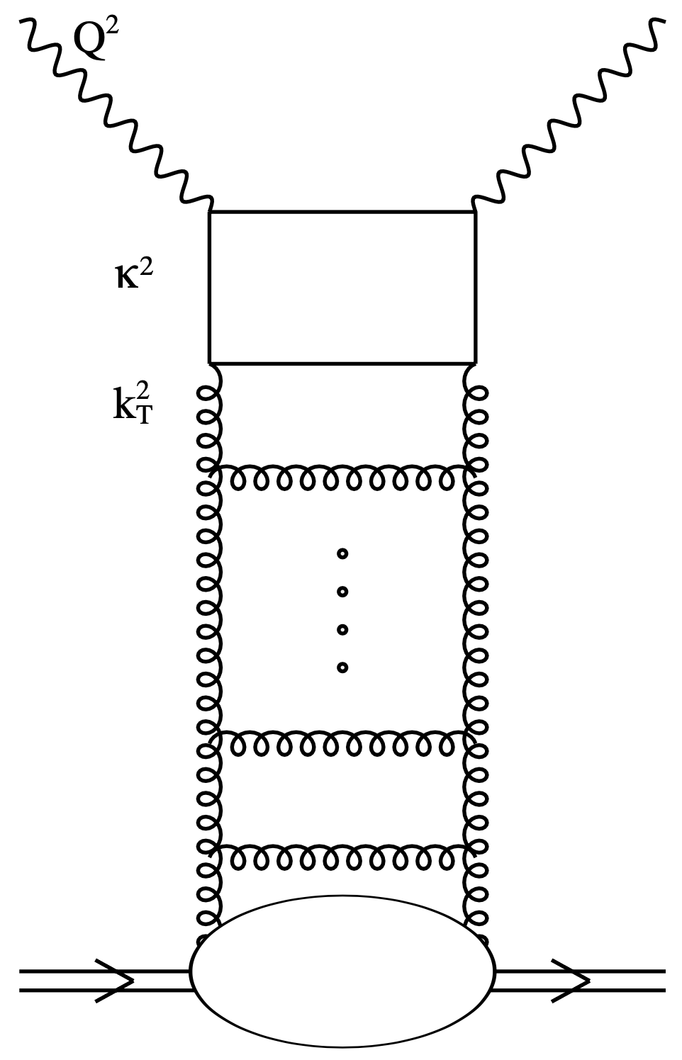
The basic process which we consider is
photon - gluon fusion, , and
the corresponding diagram in the lowest order of perturbation theory
is shown in Fig. 1.
The distinctive feature of the -factorization formula
is the fact that the gluon transverse momentum, here , is taken
into account, unlike in the collinear factorization framework,
where the integrated parton density depends only on the fraction
of the longitudinal nucleon momentum and the scale.
The photon-gluon fusion off-shell amplitude is known up to NLO accuracy [13, 14, 15]. In our model, we use the LO expression for that amplitude but with the additional corrections stemming from the exact kinematics, which effectively takes into account a part of the important higher order corrections [16, 17].
The expression for the longitudinal structure function can be written in the following form
| (1) |
where is defined by
| (2) |
The denominators are defined as
| (3) |
In Eq. (1) the sum runs over all the active quark flavours , here u, d, s, c. The is the strong coupling. The transverse momenta of the quark and gluon are denoted by and respectively, see Fig. 1. Let us define the shifted transverse momentum as follows
| (4) |
The variable is the fraction of the longitudinal momentum of the proton carried by the gluon which can be computed by taking into account the exact kinematics [18]
| (5) |
The variable is the corresponding Sudakov parameter appearing in the quark momentum decomposition into the basic light-like four vectors, and which are defined as
| (6) |
where is the target nucleon mass. We decompose four-vector as
| (7) |
where
| (8) |
The variable in (5) is the fraction of the longitudinal momentum of the proton carried by the gluon, which couples to the quarks in the ‘quark-box’, see Fig.1. In the leading order case this variable should be equal to Bjorken . This is also the case in the dipole model formulation of the high energy scattering. Here however we include the exact kinematics, which effectively makes this fraction larger than . This has significant numerical effects, as demonstrated for example in Ref. [19].
The unintegrated gluon density should in principle be obtained from an equation which resums small contributions, that is the BFKL equation. In Ref.[4] we used the approach where the unintegrated gluon density was computed from the standard integrated density by taking a logarithmic derivative
| (9) |
where satisfies the conventional (LO or NLO) DGLAP equations. In this approximation one neglects the higher order small resummation effects in the gluon density and therefore in the gluon anomalous dimension. This approximation will be used in the present update of the model111This result affects the gluon distribution only at very small values of . . We shall also use the gluon density from the Kimber-Martin-Ryskin approach [20, 21] which supplements the formula (9) with the Sudakov form-factor
| (10) |
defined as
| (11) |
with the the gluon-gluon DGLAP splitting functions. The cut-off is necessary to regulate the divergence at . As discussed in Ref.[22], different forms of the cut-off were considered in the literature: the strong ordering cut-off and the angular ordering cut-off . We checked both choices, which in our calculation do not lead to any significant differences of the results.
The parameters in Eq. (3) are the masses of the quarks. Since we are interested in the low region of the structure function, the values of the masses are important. It should be noted that the integrals defined by Eq. (2) are infrared finite even if we set . However, the non-zero values of the quark masses are necessary if formula (1) is extrapolated down to , respecting the kinematic constraint . The non-zero quark masses then play the role of the infrared regulator.
We shall consider two scenarios for the quark masses. In the first scenario we set the masses equal to where denotes the mass of the lightest vector meson which can be viewed as a component in the photon wave function. This non-perturbative Vector Meson Dominance approach can be argued within the dipole model framework. In the latter one views the DIS process as the photon fluctuating into the pair, the color dipole which then scatters off the target through the exchange of gluons. This exchange can be related to the unintegrated gluon density function, . We thus assume that the expressions for the structure function within photon-gluon fusion mechanism include also the virtual vector meson contributions. This motivates the choice of the quark masses to be related to the vector meson masses.
In the second scenario, we will treat the quark masses as parameters, which can be tuned to obtain the best description of the data at small . As we shall see in more detail in Sec. 5 masses GeV for the u, d, s quarks provide an excellent description of the experimental data from JLab at low values of , as in the dipole model [23].
Finally, it should be mentioned, that yet another process contributes to the structure function, which originates from the virtual photon-quark interactions, with the emission of a gluon, . This contribution is treated within the standard collinear approximation as in Ref. [24]. These two mechanisms will be referred to as gluon and quark contributions respectively.
4 The model for higher twist contribution
In this section we shall describe the model for the higher twist contribution to at low values of , following exactly Ref.[4]. As discussed in Sec. 2 the structure function contains significant higher twist contributions in the region of small [25, 26, 27]. Such higher twists vanish when . For example, higher twists were analyzed in the context of the dipole model, together with the saturation of the dipole cross section. It was demonstrated that this framework predicts large contributions from the higher twists to the longitudinal structure function [28, 29, 30].
The main idea of our approach [4] was to consider separately the regions of low and high transverse momenta of the quarks and the gluons in the proton. Integration over in the integral (2) is divided into the region of low and high transverse momenta, , and , respectively. Here, is an arbitrary phenomenological cut-off parameter, chosen to be of the order of 1 GeV2. We varied this parameter in the range GeV2, and found the sensitivity of the results less than about 10%.
The region of high transverse momenta is treated according to the expression from -factorization, Eq. (2). In the low region, which is likely to be dominated by the soft physics, we use the ‘on-shell’ approximation which corresponds to setting transverse momentum of the gluon to zero. This allows to cast the Eq. (2) into the collinear form with the gluon density which is obtained from an unintegrated gluon density , see Ref. [4] for details. Next, we make the substitution:
| (12) |
where is a dimensionless parameter. This leads to the following representation of the higher twist contribution to :
| (13) |
where the denominator is given by
| (14) |
The constant in Eq. (12) can be fixed from the transverse structure function, . We assume that the non-perturbative contribution to also comes from the region of low values of and is controlled by the same parameter . The term does not depend on and thus can be interpreted as representing the contribution of soft Pomeron exchange with intercept 1.
It should be noted that given by equation (13) vanishes as in the high limit (modulo logarithmically varying factors). We call it therefore a ‘higher twist contribution’. Observe that this term will also respect the kinematic constraint in the limit .
In order to find the parameter one needs to consider the transverse structure function and perform the same approximations on it as above. In the on-shell case, that is when the gluon transverse momentum is small, the corresponding formula which describes the photon - gluon contribution to the structure function is
| (15) | |||||
The soft term in is then obtained from this expression by integrating over the low region (). Finally, we perform the same substitution as in Eq. (12) and we identify this soft part of with the ‘background’ term of Ref.[18], i.e.
| (16) |
where now
| (17) |
A possible weak dependence of is neglected and we set
, see Ref.[18].
The complete structure function is represented as
where is calculated from Eqs (1) and (2) and from Eq. (13).
5 Numerical results
In this section we present numerical results for the longitudinal structure function and compare them with the experimental data.
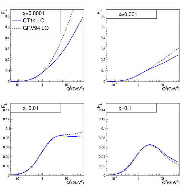
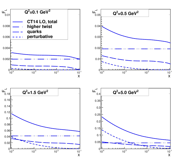
The calculated is shown in Figs 2 and 3 as function of in bins of and as function of in bins of , respectively. Two sets of the quark and gluon PDFs, both at the leading order accuracy, were used: the GRV94LO [31] (used previously in Ref. [4]) and CT14LO [32]. In the region of our interest, low and low values the results practically do not depend on that choice. We have also verified that changing from LO to NLO PDFs has negligible impact on our results in the non-perturbative region. Therefore we stick to the LO choice of the PDFs. In what follows the CT14LO parametrization222The more modern distributions, e.g. CT18 do not contain the LO PDFs. will be used.
Apart from the approach displayed in Eq. (9) we also used the unintegrated gluon density with the Sudakov form-factor, Eq. (10) and found negligible differences between these two approaches. Besides the dominant (at small ) photon-gluon fusion mechanism, we have also included a contribution from quarks, , taking into account threshold effects, for details see Ref.[4].
In the calculations we took into account the contributions from u, d, s and c quarks of masses 0.35, 0.35, 0.5 and 1.5 GeV respectively ( masses). For comparison lower quark masses equal to 0.14 GeV for u, d, s quarks were also employed (). The parameter was set to 0.8 GeV2. This value was varied in the interval 0.5 – 1.2 GeV2 which resulted in changing the by at most 10%.
In Ref. [4] we also have performed calculations within the on-shell approximation, which corresponded to setting the gluon transverse momentum to zero in the photon-gluon amplitude, Eq. (2) and restricting the integration over to . We found that the differences between off-shell and on-shell calculations are small, particularly in the low region. Therefore in this update we only stick to the off-shell calculation.
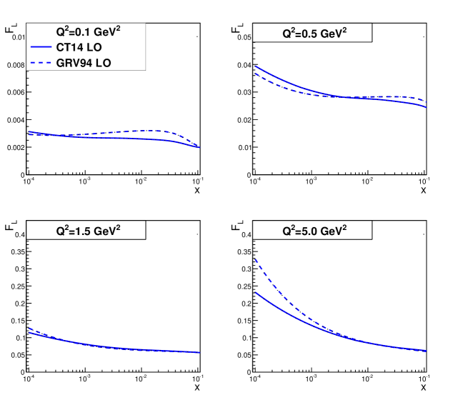
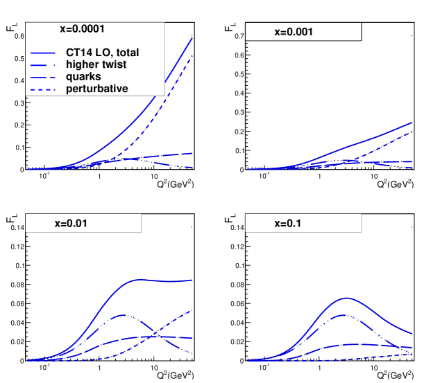
The (small) -dependence is weak at low and slightly growing with decreasing while the at low and low is very small, less than 0.005 (for GeV2) and strongly decreasing with decreasing . Contributions to from the quarks, the perturbative part and the higher twist are illustrated in Figs 4 - 5 and clearly visualize the interplay of different mechanisms in building the in our model. We note that the perturbative mechanism contributes very little in the low region.
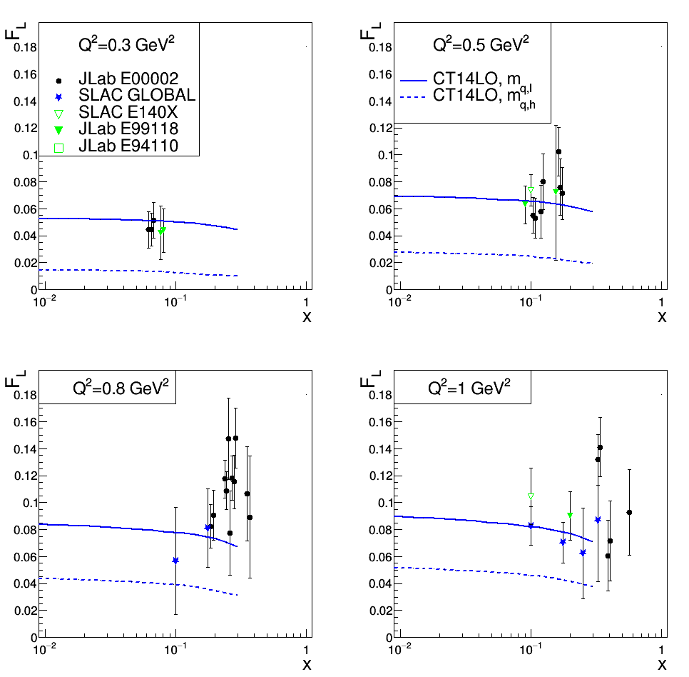
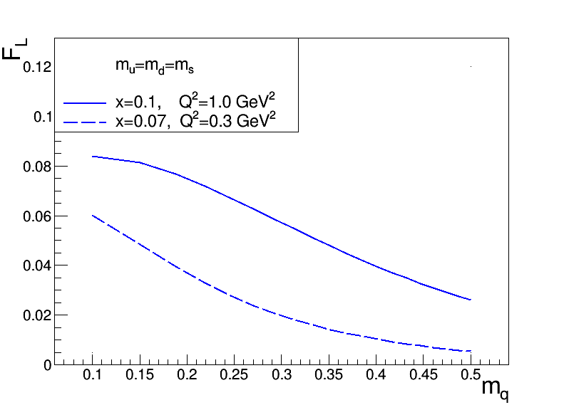
In Fig. 6 we compare the calculations with measurements. Unfortunately the latter are very scarce in the non-perturbative region, see Fig. 1 in Ref.[33] where a compilation of measurements is given. Only results from the JLab E99-118 [34], E94-110 [35], E00-002 [33], SLAC E140X [36] and SLAC GLOBAL analysis [37] extend to the edge of the low non-perturbative region. There our model with standard light quark masses clearly underestimates the data (broken line in Fig. 6). On the other hand, results for the set of low masses of the light quarks (u,d,s), GeV which were used in the dipole model calculations [23] seem to reproduce the measurements well (continuous line in Fig. 6). The strong dependence of the results on the assumed quark masses, is illustrated in Fig. 7 for two kinematic points.
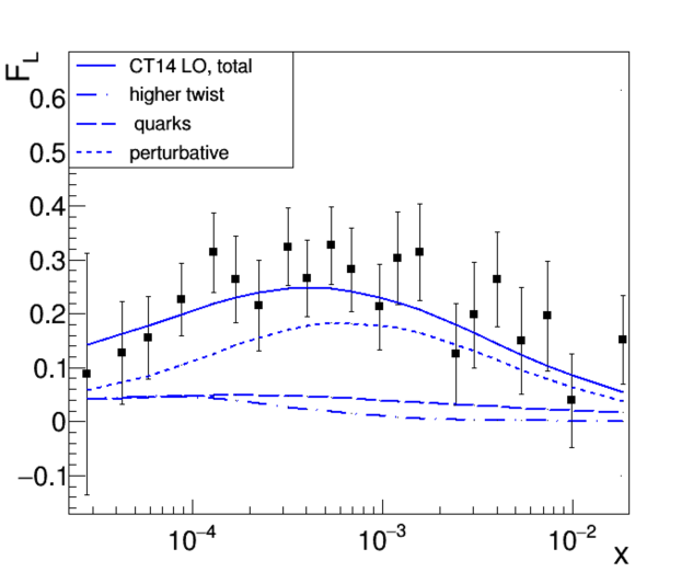
Finally, the H1 Collaboration measurements of in the perturbative region at HERA, [5] are very well reproduced, see Fig. 8.
6 Conclusions
In this paper a parametrization of the proton longitudinal structure function at low and low is presented. It is a revisit and update of the parametrization modelled in Ref.[4] and based on the photon-gluon fusion treated in the factorization, suitably extrapolated to the region of low . There is a severe need to know in this region, down to , in the electroproduction data analysis , e.g. in the QED radiative corrections. Unfortunately there are practically no measurements in this region. This leaves the modelling constrained only at the upper end of the validity interval, as (scarce) measurements are limited to 0.1 GeV2 and 0.1, the latter being the limit of applicability of our model.
The model fulfills the kinematic constraint at . It also contains a higher twist term, which can be interpreted as a soft Pomeron exchange. This term comes from the low transverse momenta of the quarks in the quark box diagram. The coupling of the soft Pomeron to the external virtual photon is modeled by a constant, which is fixed from the non-perturbative term of the transverse structure function. Thus our model for the higher twist in principle does not have any free parameters.
As in the previous version of the model we have used the prescription for the unintegrated gluon density as the logarithmic derivative of the standard integrated gluon density. The unintegrated gluon density which includes the Sudakov form-factor was also employed as an alternative. Compared to the old version of the model, we have used newer parton distributions. The updated parton distributions did not affect the results in the regime of low and low in any significant way.
The structure function turns out to be very small at 0.1 GeV2, essentially independent of at low and low and practically insensitive to the input parton distributions and perturbative accuracy (LO or NLO) of the PDFs. The model of underestimates the JLab and SLAC measurements, performed at low and unless the light quark masses are lowered down to 0.14 GeV, as in the dipole model, which brings the calculations to a very good agreement with the data. These data are however very scarce. On the other hand the model reproduces well the H1 measurements taken in the perturbative region ( 1.5 GeV2). In conclusion, we believe that the presented model will be useful at several stages of the data analysis, e.g. evaluation of the QED radiative corrections at the Electron Ion Collider.
Acknowledgments
We thank Fredrick Olness and Wojciech Słomiński for discussions; we express our gratitude to Eric Christy, Cynthia Keppel, Peter Monaghan, Ioana Niculescu, and Katarzyna Wichmann for supplying us with and discussing the measurements. AMS is supported by the U.S. Department of Energy grant No. DE-SC-0002145 and in part by National Science Centre in Poland, grant 2019/33/B/ST2/02588. The code for calculating is available upon request from the authors.
References
-
[1]
B. Badelek, D. Y. Bardin, K. Kurek and C. Scholz,
Z. Phys. C 66 (1995) 591;
doi:10.1007/BF01579633; arXiv:hep-ph/9403238. -
[2]
COMPASS Collaboration, C. Adolph, et al.,
Phys. Lett. B 753 (2016) 18;
doi: 10.1016/j.physletb.2015.11.064; arXiv:hep-ex/1503.08935. - [3] R. Abdul Khalek, et al., Science Requirements and Detector Concepts for the Electron-Ion Collider: EIC Yellow Report, arXiv:physics.ins-det/2103.05419v3.
-
[4]
B. Badelek, J. Kwiecinski and A. Stasto,
Z. Phys. C 74 (1997) 297;
doi:10.1007/s002880050391; arXiv:hep-ph/9603230. -
[5]
H1 Collaboration, V. Andreev et al.,
Eur. Phys. J. C 74 (2014) 2814;
doi:10.1140/epjc/s10052-014-2814-6; arXiv:hep-ex/1312.4821. -
[6]
S. Catani, M. Ciafaloni and F. Hautmann,
Phys. Lett. B 242 (1990) 97;
doi:10.1016/0370-2693(90)91601-7. -
[7]
S. Catani, M. Ciafaloni and F. Hautmann,
Nucl. Phys. B 366 (1991) 135;
doi:10.1016/0550-3213(91)90055-3. -
[8]
J. C. Collins and R. K. Ellis,
Nucl. Phys. B 360 (1991) 3;
doi:10.1016/0550-3213(91)90288-9. -
[9]
S. Catani and F. Hautmann,
Nucl. Phys. B 427 (1994) 475;
doi:10.1016/0550-3213(94)90636-X; arXiv:hep-ph/9405388. -
[10]
M. Ciafaloni,
Phys. Lett. B 356 (1995) 74;
doi:10.1016/0370-2693(95)00801-Q; arXiv:hep-ph/9507307. -
[11]
E. M. Levin and M. G. Ryskin,
Sov. J. Nucl. Phys. 53 (1991) 653;
LNF-90-025-PT. -
[12]
J. Blumlein,
J. Phys. G 19 (1993) 1623;
doi:10.1088/0954-3899/19/10/021. -
[13]
J. Bartels, S. Gieseke and A. Kyrieleis,
Phys. Rev. D 65 (2001) 014006;
doi:10.1103/PhysRevD.65.014006; arXiv:hep-ph/0107152. -
[14]
J. Bartels, D. Colferai, S. Gieseke and A. Kyrieleis,
Phys. Rev. D 66 (2002) 094017;
doi:10.1103/PhysRevD.66.094017; arXiv:hep-ph/0208130v2. -
[15]
I. Balitsky and G. A. Chirilli,
Phys. Rev. D 87 (2013) 014013;
doi:10.1103/PhysRevD.87.014013; arXiv:1207.3844 [hep-ph]. -
[16]
A. Bialas, H. Navelet and R. B. Peschanski,
Nucl. Phys. B 593 (2001) 438;
doi:10.1016/S0550-3213(00)00640-4; arXiv:hep-ph/0009248. -
[17]
A. Bialas, H. Navelet and R. B. Peschanski,
Nucl. Phys. B 603 (2001) 218;
doi:10.1016/S0550-3213(01)00153-5; arXiv:hep-ph/0101179. -
[18]
A. J. Askew, J. Kwiecinski, A. D. Martin and P. J. Sutton,
Phys. Rev. D 47 (1993) 3775;
doi:10.1103/PhysRevD.47.3775. -
[19]
K. Golec-Biernat and A. M. Stasto,
Phys. Rev. D 80 (2009) 014006;
doi:10.1103/PhysRevD.80.014006; arXiv:0905.1321 [hep-ph]. -
[20]
M. A. Kimber, A. D. Martin and M. G. Ryskin,
Eur. Phys. J. C 12 (2000) 655;
doi:10.1007/s100520000326; arXiv:hep-ph/9911379v2. -
[21]
M. A. Kimber, A. D. Martin and M. G. Ryskin,
Phys. Rev. D 63 (2001) 114027;
doi:10.1103/PhysRevD.63.114027; arXiv:hep-ph/0101348. -
[22]
K. Golec-Biernat and A. M. Stasto,
Phys. Lett. B 781 (2018) 633;
doi:10.1016/j.physletb.2018.04.061; arXiv:1803.06246 [hep-ph]. -
[23]
K. J. Golec-Biernat and M. Wusthoff,
Phys. Rev. D 59 (1998) 014017;
doi:10.1103/PhysRevD.59.014017; arXiv:hep-ph/9807513;
K. J. Golec-Biernat and S. Sapeta, JHEP 03 (2018) 102;
doi:10.1007/JHEP03(2018)102; arXiv:1711.11360 [hep-ph]. -
[24]
G. Altarelli and G. Martinelli,
Phys. Lett. B 76 (1978) 89;
doi:10.1016/0370-2693(78)90109-0. -
[25]
J. L. Miramontes, M. A. Miramontes and J. Sanchez Guillen,
Phys. Rev. D 40 (1989) 2184;
doi:10.1103/PhysRevD.40.2184. -
[26]
J. Sanchez Guillen, et al.,
Nucl. Phys. B 353 (1991) 337;
doi:10.1016/0550-3213(91)90340-4. -
[27]
S. I. Alekhin,
Eur. Phys. J. C 12(2000) 587;
doi:10.1007/s100520000179; arXiv:hep-ph/9902241. -
[28]
J. Bartels, K. J. Golec-Biernat and K. Peters,
Eur. Phys. J. C 17 (2000) 121;
doi:10.1007/s100520000429; arXiv:hep-ph/0003042v4. -
[29]
J. Bartels, K. Golec-Biernat and L. Motyka,
Phys. Rev. D 81 054017 (2010) 054017;
doi:10.1103/PhysRevD.81.054017; arXiv:0911.1935 [hep-ph]. -
[30]
L. Motyka, M. Sadzikowski, W. Słomiński and K. Wichmann,
Eur. Phys. J. C 78 (2018) 80;
doi:10.1140/epjc/s10052-018-5548-z; arXiv:1707.05992 [hep-ph]. -
[31]
M. Glück, E. Reya and A. Vogt, Z. Phys. C 67 (1995) 433;
doi:10.1007/BF01624586. -
[32]
A. Buckley, et al., Phys. J. C 75 (2015) 132;
doi:10.1140/epjc/s10052-015-3318-8; arXiv:1412.7420v2 [hep-ph]. -
[33]
JLab E00-002 Collaboration, V. Tvaskis,
et al.,
Phys. Rev. C 97 (2018) 045204;
doi:10.1103/PhysRevC.97.045204; arXiv:1606.02614 [nucl-ex]. -
[34]
JLab E99-118 Collaboration, V. Tvaskis, et al.,
Phys.Rev.Lett. 98 (2007) 142301;
doi:10.1103/PhysRevLett.98.142301; arXiv:nucl-ex/0611023. -
[35]
JLab E94-110 Collaboration, Y. Liang, et al.,
arXiv:nucl-ex/0410027v2;
Y. Liang, PhD thesis, The American University (2003). -
[36]
SLAC E140X Collaboration, L. H. Tao et al.,
Z. Phys. C 70 (1996) 387;
doi:10.1007/s002880050117. -
[37]
L. W. Whitlow, et al.,
Phys. Lett. B 282 (1992) 475;
doi:10.1016/0370-2693(92)90672-Q.