Lorenz fields convey energy as Nadelstrahlung

As representative Lorenz potential augmentations consider

When $f$, $g$ and $h$ are functionally dependent only on phase factors $\omega t-\mathbf{k}\bullet\mathbf{r}$ where $\mathbf{k}=(k_{x},k_{y},k_{z})$ and $a^{2}k^{2}=\omega^{2}$, these potentials satisfy the homogeneous wave equation and the Lorenz condition. Since $\boldsymbol{\nabla}\Omega_{0}=-\mathring{\Omega}_{0}\mathbf{k}/\omega$ and $\mathbf{k}\times(\mathbf{k}\times\mathring{\mathbf{A}}_{0})=\mathbf{k}(\mathbf{k}\bullet\mathring{\mathbf{A}}_{0})-k^{2}\mathring{\mathbf{A}}_{0}$,

When the vector potential components are periodic functions they can be considered to be plane waves. Unlike Lorenz fields defined by nonlocal potentials, the polarizations are local functions. They are orthogonal, $\mathbf{P}\bullet\mathbf{M}=0$, and have no longitudinal components, $\mathbf{k}\bullet\mathbf{P}=\mathbf{k}\bullet\mathbf{M}=0$; they carry a flux $\mathbf{M}\times\mathbf{P}=\omega^{-2}(\mathbf{k}\times\mathring{\mathbf{A}}_{0})^{2}\mathbf{k}/k$ equal to $\mathbf{D}\times\mathbf{H}$ when $\mathbf{E}=\mathbf{B}=0$ and travel indefinitely in a ray direction $\mathbf{k}$ at speed $a$ without driving sources.

Polarization waves provide, at least, a classical solution to the [7, 8, 9, 21] duality. To see how, consider a vector potential with Lissajous phases $\phi_{1}=\omega_{1}t-\mathbf{k}_{1}\bullet\mathbf{r}$, $\phi_{2}=\omega_{2}t-\mathbf{k}_{2}\bullet\mathbf{r}$ and $\phi_{3}=\omega_{3}t-\mathbf{k}_{3}\bullet\mathbf{r}$ where $\mathbf{k}_{1}=(k_{1x},k_{1y},0)$, $\mathbf{k}_{2}=(k_{2x},k_{2y},0)$ and $\mathbf{k}_{3}=(0,0,k_{3z})$. Though periodic components are not essential, added insight is provided by the simple form

This also satisfies the homogeneous wave equation $\square_{a}\Omega_{0}=0$. So these potentials can be taken to define the Eqs. (5) Lorenz polarizations and flux given in the Appendix.

When $\phi_{1}=\phi_{2}=\phi$ for $\mathbf{k}_{1}\neq\mathbf{k}_{2}$ the phase moves on the parametric line

with velocity

giving $V^{2}=2a^{2}k_{1}k_{2}[k_{1}k_{2}-(k_{1x}k_{2x}+k_{1y}k_{2y})]/(k_{1x}k_{2y}-k_{2x}k_{1y})^{2}$. If the flux vector were to have a component perpendicular to the phase velocity the ray would dissipate. So the vector product components must vanish or, for the Eqs. (17c) and (13) flux and velocity,

This reduces to $(k_{1y}+k_{2x})[k_{1}k_{2}-(k_{1x}k_{2x}+k_{2y}k_{1y})]=0$. So, $\mathbf{k}_{1}$ and $\mathbf{k}_{2}$ can satisfy two alternative conditions for flux and phase velocity directions to be aligned. The phase $\phi$ is a parameter that gives simple harmonic polarizations. But $\phi$ is not a wave phase factor unless $\omega_{1}=\omega_{2}$, because it is confined to the line defined by Eqs. (12). As $\mathbf{k}_{1}\to\mathbf{k}_{2}$, the ray-like character persists.

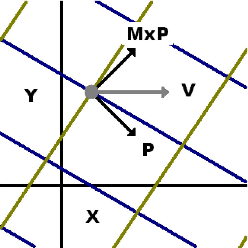
Although the case for $\mathbf{k}_{1}\neq\mathbf{k}_{2}$would appear to have physical relevance in describing light-like waves, the more general case in which $\phi_{1}\neq\phi_{2}$ may provide a particle description for light. In this case, the phase point $(\phi_{1},\phi_{2})$ moves on a path defined by Eqs. (12) with $\phi$ replaced by $\phi_{1}$ or $\phi_{2}$. Now, the flux has the Eq. (16c) form. To prevent ray dissipation by flux components normal to the phase path, restraints must again be applied to $\mathbf{k}_{1}$ and $\mathbf{k}_{2}$. These will depend on $\phi_{1}$ and $\phi_{2}$. This means the flux is carried by phase points. This case is illustrated in Fig. 1 for select wave vector values that give $\mathbf{V}=(a,0,0)$. Construction details are given in the caption. Significantly, Fig. 1 shows that $V$ can equal $a$ even when $\mathbf{V}$ and $\mathbf{M}\times\mathbf{P}$ are not aligned. The concentrated energy bearers can be marshaled into ensembles.

Early last century, H. A. Lorentz (1853-1928) made two comments on Maxwell field potentials. First, the Eqs. (4) electric field strength and magnetic induction are unchanged in form for any gauge function, $\chi$, that gives new potentials defined by

Gauge restraints are now widely accepted [10]. Some gauges do not even specify a gauge function. For these, a gauge function further restrains the potentials. The second comment was that Eq. (1), dubbed the Lorentz condition, causes the Maxwell field potentials to satisfy the Eqs. (2) wave equations. This is shown in [11]. Lorentz did not relate these comments. So, the Lorentz condition has been treated as a gauge that can be freely changed. This freedom and wave function potential nonlocality have caused potential reality to be denied. When Eq. (1) is charge conservation, as I have shown above that it is, these comments are coupled. As charge conservation, Eq. (1) is a basic law. With this, in Sec. 2 I have shown the Eqs. (2) wave function potentials give the Eq. (6) field equations with Maxwell form. This is the second comment converse. Thus, Maxwell fields must always have wave function potentials. The potentials can be local, nonlocal or mixed. Further, as a basic law, Eq. (1) can not be freely changed.

When the original potentials are sourced wave functions Eqs. (15) resolve to three Lorenz classes that need not have the gauge function form. First, the new potentials are not wave functions. Second, the new potentials are wave functions with changed source values. Third, the new potentials are wave functions with unchanged source values. In the first case the Lorentz condition will not apply. Then, charge will not be conserved and the potentials will not propagate with a wave speed. Both must be spurned. The latter, because tests in [12, 13, 14, 15] show longitudinal electric fields to propagate with finite speed. The last two cases will conserve charge if the Lorentz condition persists. This persistence will assure Lorenz field equations in which charge and current density are deemed observables that produce potentials and fields yielding emergent light-like waves. These conserve charge progressively as described in Sec. 3.1. Further, localized energy is conveyed on ray forming phase points as described in Sec. 3.2. For gauge transformations, persistence requires the Lorenz gauge, $\square_{a}\chi\equiv\boldsymbol{\nabla}\bullet\boldsymbol{\nabla}\chi-\overset{\circ\circ}{\chi}/a^{2}=0$. It suppresses the polarizations and, thus, their dependent, emergent rays.

In the late eighteen hundreds, H. von Helmholtz (1821-94) tried to unite electromagnetic theories [16]. To this end he based his concept on electric and magnetic polarization. From this he obtained wave equations for a homogeneous medium. His transverse waves have speed $c/\sqrt{\epsilon\mu}$. Here $c$ is the vacuum light speed. Only difficult, precision measurements could complete the theory, because his longitudinal wave speed has any value greater than or equal to zero. Unlike Helmholtz waves, Lorenz waves are simply transverse, because Eq. (6b) gives $\boldsymbol{\nabla}\bullet\mathbf{P}=0$.

To promote his concept, Helmholtz issued a challenge to measure a coupling between electromagnetism and dielectric polarization. His former student, H. Hertz (1857-94), later claimed the prize. He then went on to observe dipole radiation reflection and interference. Based on this Hertz concluded that polarization propagation is like vacuum light [17, pp. 19 and 122-3] and [18]. Hertz’s dipole field [4, 17, 18] has radial, transverse wave emergence in the far field. At intermediate distances the waves have greater than light speed that approaches light speed in the far field. These waves change from longitudinal to transverse as the radial direction changes from dipole length to dipole equator. Hertz reconciled these properties in the equatorial plane by observing strobed interference between free air and straight wire waves [17, pp. 150-5]. His and recent [19] reports suggest light structure may be open to study. Antiphased fields in [19] may represent an Eq. (6d) Ampere law based, magnetoinductive internal structure [2].

For vacuum polarization waves Eq. (8a) takes a simple form. By the Gauss theorem, it represents an equality between the temporal energy change in a volume and the energy flux through its surface. For monochromatic waves, $\mathbf{M}\times\mathbf{P}$ can be written using the Hertz analogy as $h\nu\mathbf{f}$ where $h\nu$ is photon energy and $\mathbf{f}$ is photon flux with coherence length inversely related to monochromaticity departure [20]. This dependence means that the photon power density must approach zero as the coherence length becomes very large for monochromatic photons. The compact, quantum particle photon concept is untenable in this limit. The concept is further threaten by confounding photon size with wavelength. This problem is revealed by the Table 1 benchmarks. There the lowest energy photons have a wavelength greater than the Earth orbit radius. These conflicts are homologized in [21] by setting a hypothetical photon energy density equal to a flux magnitude divided by the energy transfer speed.

When phase point motion and wave flux are not aligned, flux normal to the phase point motion would force ray dissipation. This is like saying that all light rays are electromagnetic, but not all electromagnetic waves are light rays. Failure to recognize this has prevented light-like rays from being found in electromagnetic fields to help describe light behavior in optics and photography [7, 8, 9]. Synchrotron light emitted as rays by high speed electrons in a circular orbit supports this. These rays are attributed to the radial acceleration not the periodic linear acceleration required to maintain the electron energy. Their presence in the electric field has not been shown [22, 23, 24]. However, one unconfirmed report [25] finds them to be electrically polarized in the electron orbit plane like the Sec. 3.2 phase directed polarization waves.

Although phase independence is compelling, its nonexistence would support treating rays as having the closely bound potentials described in Sec. 3.1 above. In this limit energy should still be borne progressively by charge conserving phase points. Even so, phase independence is a hidden variable whose consequence is unintuitive. Whether electromagnetic energy localization to phase points is consistent with quantum statistics should be examined elsewhere, because it has special features to help model the standard quantum oscillators. The points are defined by Lissajous potentials. They bear a fixed flux at constant speed. They vanish where either charge cannot be conserved or flux and phase are not aligned. Individually, they do not bear oscillations. But they can be marshaled into Eq. (20), Piekara bead-chain, flux magnitude beads. These features provide a new means to help describe light generation. If flux and phase alignment were required for light generation, its low intrinsic likelihood would predict a small efficiency. One challenge is light from atoms. Its study could help increase laser output when atoms are aligned by shell structure.