Lossy Compression in Near-Linear Time
via Efficient Random Codebooks and Databases
Abstract
The compression-complexity trade-off of lossy compression algorithms that are based on a random codebook or a random database is examined. Motivated, in part, by recent results of Gupta-Verdú-Weissman (GVW) and their underlying connections with the pattern-matching scheme of Kontoyiannis’ lossy Lempel-Ziv algorithm, we introduce a non-universal version of the lossy Lempel-Ziv method (termed LLZ). The optimality of LLZ for memoryless sources is established, and its performance is compared to that of the GVW divide-and-conquer approach. Experimental results indicate that the GVW approach often yields better compression than LLZ, but at the price of much higher memory requirements. To combine the advantages of both, we introduce a hybrid algorithm (HYB) that utilizes both the divide-and-conquer idea of GVW and the single-database structure of LLZ. It is proved that HYB shares with GVW the exact same rate-distortion performance and implementation complexity, while, like LLZ, requiring less memory, by a factor which may become unbounded, depending on the choice or the relevant design parameters. Experimental results are also presented, illustrating the performance of all three methods on data generated by simple discrete memoryless sources. In particular, the HYB algorithm is shown to outperform existing schemes for the compression of some simple discrete sources with respect to the Hamming distortion criterion.
Keywords — Lossy data compression, rate-distortion theory, pattern matching, Lempel-Ziv, random codebook, fixed database
1 Introduction
One of the last major outstanding classical problems of information theory is the development of general-purpose, practical, efficiently implementable lossy compression algorithms. The corresponding problem for lossless data compression was essentially settled in the late 1970s by the advance of the Lempel-Ziv (LZ) family of algorithms [58][56][59] and arithmetic coding [42][39][26]; see also the texts [20][5]. Similarly, from the early- to mid-1990s on, efficient channel coding strategies emerged that perform close to capacity, primarily using sparse graph codes, turbo codes, and local message-passing decoding algorithms; see, e.g., [47][30][44][31], the texts [15][29][40], and the references therein.
For lossy data compression, although there is a rich and varied literature on both theoretical results and practical compression schemes, near-optimal, efficiently implementable algorithms are yet to be discovered. From rate-distortion theory [6][43] we know that it is possible to achieve a sometimes dramatic improvement in compression performance by allowing for a certain amount of distortion in the reconstructed data. But the majority of existing algorithms are either compression-suboptimal or they involve exhaustive searches of exponential complexity at the encoder, making them unsuitable for realistic practical implementation.
Until the late 1990s, most of the research effort was devoted to addressing the issue of universality, see [23] and the references therein, as well as [55][37][57][38][36][53][54][49]; algorithms emphasizing more practical aspects have been proposed in [51]. In addition to many application-specific families of compression standards (e.g., JPEG for images and MPEG for video), there is a general theory of algorithm design based on vector quantization; see [16][27][7][17] and the references therein. Yet another line of research, closer in spirit to the present work, is on lossy extensions of the celebrated Lempel-Ziv schemes, based on approximate pattern matching; see [35][45][52][28][2][50][3][13][24][1].
More recently, there has been renewed interest in the compression-complexity trade-off, and in the development of low-complexity compressors that give near-optimal performance, at least for simple sources with known statistics. The lossy LZ algorithm of [24] is rate-distortion optimal and of polynomial complexity, although, in part due the penalty paid for universality, its convergence is slow. For the uniform Bernoulli source, [33][34][32] present codes based on sparse graphs, and, although their performance is promising, like earlier approaches they rely on exponential searches at the encoder. In related work, [46][8] present sparse-graph compression schemes with much more attractive complexity characteristics, but suboptimal compression performance. Rissanen and Tabus [41] describe a different method which, unlike most of the earlier approaches, is not based on a random (or otherwise exponentially large) codebook. It has linear complexity in the encoder and decoder and, although it appears to be rate-distortion suboptimal, it is an effective practical scheme for Bernoulli sources. Sparse-graph codes that are compression-optimal and of subexponential complexity are constructed in [18]. A simulation-based iterative algorithm is presented in [22] and it is shown to be compression-optimal, although its complexity is hard to evaluate precisely as it depends on the convergence of a Markov chain Monte Carlo sampler. The more recent work [21] on the lossy compression of discrete Markov sources also contains promising results; it is based on the combination of a Viterbi-like optimization algorithm at the encoder followed by universal lossless compression.
The present work is partly motivated by the results reported in [19] by Gupta-Verdú-Weissman (GVW). Their compression schemes are based on the “divide-and-conquer” approach, namely the idea that instead of encoding a long message using a classical random codebook of blocklength , it is preferable to break up into shorter sub-blocks of shorter length , say, and encode the sub-blocks separately. The main results in [19] state that, with an appropriately chosen sub-block length , it is possible to achieve asymptotically optimal rate-distortion performance with near-linear implementation complexity (in a sense made precise in Section 3 below).
Our starting point is the observation that there is a closely related, in a sense dual, point of view. On a conceptual as well as mathematical level, the divide-and-conquer approach is very closely related to a pattern-matching scheme with a restricted database. In the divide-and-conquer setting, given a target distortion level and an , each sub-block of length in the original message is encoded using a random codebook consisting of codewords, where is the rate-distortion function of the source being compressed (see the following section for more details and rigorous definitions). To encode each sub-block, the encoder searches all entries of the codebook, in order to find the one which has the smallest distortion with respect to that sub-block.
Now suppose that, instead of a random codebook, the encoder and decoder share a random database with length , generated from the same distribution as the Shannon-optimal codebook. As in [24], the encoder searches for the longest prefix of the message that matches somewhere in the database with distortion or less. Then the prefix is described to the decoder by describing the position and length of the match in the database, and the same process is repeated inductively starting at . Although the match-length is random, we know [13][24] that, asymptotically, it behaves like,
Therefore, because the length of the database was chosen to be , in effect both schemes will individually encode sub-blocks of approximately the same length , and will also have comparable implementation complexity at the encoder.111It is well-known that the main difficulty in designing effective lossy compressors is in the implementation complexity of the encoder. Therefore, in all subsequent results dealing with complexity issues we focus on the case of the encoder. Moreover, it is easy to see that the decoding complexity of all the schemes considered here is linear in the message length.
Thus motivated, after reviewing the GVW scheme in Section 2 we introduce a (non-universal) version of the lossy LZ scheme in [24], termed LLZ, and we compare its performance to that of GVW. Theorem 1 shows that LLZ is asymptotically optimal in the rate-distortion sense for compressing data from a known discrete memoryless source with respect to a single-letter distortion criterion. Simulation results are also presented, comparing the performance of LLZ and GVW on a simple Bernoulli source. These results indicate that for blocklengths around 1000 bits, GVW offers better compression than LLZ at a given distortion level, but it requires significantly more memory for its execution. [The same findings are also confirmed in the other simulation examples presented in Section 4.]
In order to combine the different advantages of the two schemes, in Section 3 we introduce a hybrid algorithm (HYB), which utilizes both the divide-and-conquer idea of GVW and the single-database structure of LLZ. In Theorems 2 and 3 we prove that HYB shares with GVW the exact same rate-distortion performance and implementation complexity, in that it operates in near-linear time at the encoder and linear time at the decoder. Moreover, like LLZ, the HYB scheme requires much less memory, by an unbounded factor, depending on the choice of parameters in the design of the two algorithms. Experimental results are presented in Section 4, comparing the performance of GVW and HYB. These confirm the theoretical findings, and indicate that HYB outperforms existing schemes for the compression of some simple discrete sources with respect to the Hamming distortion criterion. The earlier theoretical results stating that HYB’s rate-distortion performance is the same as GVW’s are confirmed empirically, and it is also shown that, again for blocklengths of approximately 1000 symbols, the HYB scheme requires much less memory, by a factor ranging between 15 and 240.
2 The GVW and LLZ algorithms
After describing the basic setting within which all later results will be developed, in Section 2.2 we recall the divide-and-conquer idea of the GVW scheme, and in Section 2.3 we present a new, non-universal lossy LZ algorithm and examine its properties.
2.1 The setting
Let be a memoryless source on some finite alphabet and suppose that its distribution is described by a known probability mass function on . The objective is to compress with respect to a sequence of single-letter distortion criteria,
where is an arbitrary source string to be compressed, is a potential reproduction string taking values in a finite reproduction alphabet , and is an arbitrary distortion measure. We make the customary assumption that for any source letter there is a reproduction letter with zero distortion,
The best achievable rate at which data from the source can be compressed with distortion not exceeding is given by the rate-distortion function [43][6][9],
| (1) |
where denotes the mutual information between a random variable with the same distribution as the source and a random variable with conditional distribution given .222The mutual information, rate-distortion function, and all other standard information-theoretic quantities here and throughout are expressed in bits; all logarithms are taken to be in base 2, unless stated otherwise. Let ; in order to avoid the trivial case where is identically equal to zero, is assumed to be strictly positive. It is well-known and easy to check that, for all distortion values in the nontrivial range , there is a conditional distribution that achieves the infimum in (1), and this induces a distribution on via , for all . With a slight abuse of terminology (as may not be unique) we refer to as the optimal reproduction distribution at distortion level . Recall also the analogous definition of the distortion-rate function of the source; cf. [6][9].
2.2 The GVW algorithm
The GVW algorithm333To be more precise, this is one of two closely related schemes discussed in [19]; see the relevant comments in Section 3. is a fixed-rate, variable-distortion code of blocklength and target distortion . It is described in terms of two parameters; a “small” , and an integer so that .
Given the target distortion level , let , and take,
| (2) |
First a fixed-rate code of blocklength and rate is created according to Shannon’s classical random codebook construction. Letting denote the optimal reproduction distribution at level , the codebook consists of i.i.d. codewords of length , each generated i.i.d. from . Writing , as the concatenation of sub-blocks, each sub-block is matched to its -nearest neighbor in the codebook, and it is described to the decoder using bits to describe the index of that nearest neighbor in the codebook.
This code is used times, once on each of the sub-blocks, to produce corresponding reconstruction strings , for . The description of is the concatenation of the descriptions of the individual sub-blocks, and the reconstruction string itself is the concatenation of the corresponding reproduction blocks, . The overall description length of this code is bits, so the (fixed) rate of this code is bits/symbol, and its (variable) distortion is .
2.3 The lossy Lempel-Ziv algorithm LLZ
The LLZ algorithm described here can be seen as a simplified (in that it is non-universal) and modified (to facilitate the comparison below) version of the algorithm in [24]. It is a fixed-distortion, variable-rate code of blocklength , described in terms of three parameters; an integer blocklength , and “small” .444Note that in [24] a fixed-rate, variable-distortion universal code is also described, but we restrict attention here to the conceptually simpler fixed-distortion algorithm. The algorithm will be presented in a setting “dual” to that of the GVW algorithm, in the sense that was described in the Introduction. The main difference is that the source sting will be parsed into substrings of variable length, not of fixed length .
Given and a target distortion level , define , take,
and let denote the optimal reproduction distribution at level . Then generate a single i.i.d. database of length,
| (3) |
and make it available to both the encoder and decoder.
The encoding algorithm is as follows: The encoder calculates the length of the longest match (up to -many symbols) of an initial portion of the message , within distortion , in the database. Let denote the length of this longest match,
and let denote the initial phrase of length in Then the encoder describes to the decoder:
-
the length ; this takes bits;
-
the position in the database where the match occurs; this takes bits.
From and the decoder can recover the string which is within distortion of .
Alternatively, can be described with zero distortion by first describing its length as before, and then describing itself directly using,
| (4) |
The encoder uses whichever one of the two descriptions is shorter. [Note that is not necessary to add a flag to indicate which one was chosen; the decoder can simply check if is larger or smaller than .] Therefore, from , , and (4) the length of the description of is,
| (5) |
After has been described within distortion , the same process is repeated to encode the rest of the message: The encoder finds the length of the longest string starting at position in that matches within distortion into the database, and describes to the decoder by repeating the above steps. The algorithm is terminated, in the natural way, when the entire string has been exhausted. At that point, has been parsed into distinct phrases , each of length , with the possible exception of the last phrase, which may be shorter. Since each substring is described within distortion , also the concatenation of all the reproduction strings, call it , will be within distortion of .
The distortion achieved by this code is , and it is guaranteed to be by construction. Regarding the rate, if we write for the overall description length of , then from (5),
| (6) |
and the rate achieved by this code is bits/symbol.
Remark. As mentioned in the Introduction, there are two main differences between the GVW algorithm and the LLZ scheme. The first one is that while the GVW is based on a Shannon-style random codebook, the LLZ uses an LZ-type random database. The second is that GVW divides up the message into fixed-length sub-blocks of size , whereas LLZ parses into variable-length strings of (random) lengths . But there is also an important point of solidarity between the two algorithms. Recall [14, Theorem 23] that, for large , the match length behaves logarithmically in the size of the database; that is, with high probability,
where the second approximation follows by the choice of and of Therefore, both algorithms end up parsing the message into sub-blocks of length symbols.
Our first result shows that LLZ is asymptotically optimal in the usual sense established for fixed-database versions of LZ-like schemes; see [48][24]. Specifically, it is shown that by taking large enough and small enough, the LLZ comes arbitrarily close to any optimal rate-distortion point . Note that is a parameter that simply controls the complexity of the best-match search, and its influence on the rate-distortion performance is asymptotically irrelevant.
Theorem 1. [LLZ Optimality]
Suppose the LLZ with parameters
and is used
to compress a memoryless source
with rate-distortion function
at a target distortion rate .
For any ,
the parameter
can be chosen small enough
such that:
(a) For any choice of and
any blocklength
the distortion achieved by LLZ
is no greater than
(b) Taking large enough,
the asymptotic rate of LLZ achieves
the rate-distortion bound, in that,
| (7) |
where the expectation is over all databases. Therefore, also,
| (8) |
with the expectation here being over both the message and the databases.
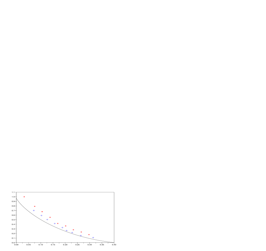
Next, the performance of LLZ is compared with that of GVW on data generated from a Bernoulli source with parameter and with respect to Hamming distortion. Simulation results at different target distortions are shown in Figure 1 and Table 1; see Section 4 for details on the choice of parameter values. It is clear from these results that, at the same distortion level, the GVW algorithm typically gives a better rate than LLZ. In terms of implementation complexity, the two algorithms have comparable execution times, but the LLZ uses significantly less memory. The same pattern – GVW giving better compression but using much more memory than LLZ – is also confirmed in the other examples we consider in Section 4.
Note that, like for the case of GVW, more can be said about the implementation complexity of LLZ and how it depends on the exact choice of parameters and . But since, as we will see next, the performance of both algorithms is dominated by that of a different algorithm (HYB), we do not pursue this direction further.
| Bern(0.4) source, Hamming distortion | |||||
|---|---|---|---|---|---|
| Performance parameters | |||||
| Algorithm | rate | memory | time | ||
| GVW | 0.05 | 0.07143 | 0.70095 | 26MB | 27m53s |
| GVW | 0.08 | 0.10286 | 0.59143 | 23MB | 21m11s |
| GVW | 0.11 | 0.12667 | 0.50381 | 27MB | 20m48s |
| GVW | 0.14 | 0.15714 | 0.41619 | 31MB | 19m52s |
| GVW | 0.17 | 0.18857 | 0.32857 | 36MB | 18m48s |
| GVW | 0.2 | 0.20571 | 0.26286 | 46MB | 19m18s |
| GVW | 0.23 | 0.22857 | 0.21905 | 57MB | 18m42s |
| GVW | 0.26 | 0.26381 | 0.15333 | 79MB | 19m46s |
| GVW | 0.29 | 0.31429 | 0.10952 | 113MB | 20m29s |
| LLZ | 0.05 | 0.03238 | 1.00029 | 1.5MB | 4m23s |
| LLZ | 0.08 | 0.07524 | 0.79129 | 1.28MB | 6m15s |
| LLZ | 0.11 | 0.10571 | 0.6754 | 1.46MB | 8m53s |
| LLZ | 0.14 | 0.1381 | 0.55171 | 1.69MB | 11m18s |
| LLZ | 0.17 | 0.16952 | 0.41827 | 2.6MB | 18m15s |
| LLZ | 0.2 | 0.2019 | 0.36381 | 3.6MB | 20m09s |
| LLZ | 0.23 | 0.23333 | 0.27975 | 6.2MB | 41m32s |
| LLZ | 0.26 | 0.26571 | 0.23102 | 13MB | 63m56s |
| LLZ | 0.29 | 0.29714 | 0.1741 | 47MB | 165m54s |
3 The HYB algorithm
In order to combine the rate-distortion advantage of GVW with the memory advantage of LLZ, in this section we introduce a hybrid algorithm and examine its performance.
The new algorithm, termed HYB, uses the divide-and-conquer approach of GVW, but based on a random database like the LLZ instead of a random codebook. It is a fixed-rate, variable-distortion code of blocklength and target distortion , and it is described in terms of two parameters; a “small” , and an integer so that .
Like with the GVW, given a target distortion level , let and take as in (2). Now, like for the LLZ algorithm, let as in (3), and generate a random database , where the are drawn i.i.d. from the optimal reproduction distribution at level . The database is made available to both the encoder and the decoder, and the message to be compressed is parsed into non-overlapping blocks, .
The first sub-block is matched to its -nearest neighbor in the database, where we consider each possible , as a potential reproduction word. Then is described to the decoder by describing the position of its matching reproduction block in the database using bits, and the same process is repeated on each of the sub-blocks, to produce reconstruction strings. The description of is the concatenation of the descriptions of the individual sub-blocks, and the reconstruction string itself is the concatenation of the corresponding reproduction blocks. The overall description length of this code is bits.
The following result shows that the HYB algorithm shares the exact same rate-distortion performance, as well as the same implementation complexity characteristics, as the GVW. Let:
Theorem 2. [HYB Compression/Complexity Trade-off] Consider a memoryless source with rate-distortion function , which is to be compressed at target distortion level . There exists an such that, for any , the HYB algorithm with parameters and as in (12) achieves a rate of bits/symbol, its expected distortion is less than , and moreover:
– Encoding time per source symbol is proportional to ,
– Decoding time per symbol is independent of and ,
where and are independent of and .
Remarks.
1. Theorem 2 is an exact analog of Theorem 1 proved for GVW in [19], the only difference being that we consider average distortion instead of the probability-of-excess distortion criterion. The reason is that, instead of presenting an existence proof for an algorithm with certain desired properties, here we examine the performance of the HYB algorithm itself. Indeed, the proof of Theorem 2 can easily be modified to prove the stronger claim that there exists some instance of the random database such that, using that particular database, the HYB algorithm also has the additional property that the probability of excess distortion vanishes as . The same comments apply to Theorem 3 below.
2. In [19] a similar result is proved with the roles and and interchanged. In fact, it should be pointed out that the scheme we call “the” GVW algorithm here corresponds to the scheme used in the proof of [19, Theorem 1]. A slight variant (having to do with the choice of parameter values and not with the mechanics of the algorithm itself) is used to prove [19, Theorem 2]. Having gone over the proofs, it would be obvious to the reader that, once the corresponding changes are made for HYB, an analogous result can be proved for HYB. The straightforward but tedious details are omitted.
3. In terms of memory, the GVW scheme requires reproduction symbols for storing the codebook, while using the same memory parameters the HYB algorithm needs symbols. The ratio between the two is,
so that the GVW needs times more memory than HYB. Moreover, the closer we require the algorithm to come to achieving an optimal point, the smaller the values of and need to be taken in Theorem 2, and the larger the corresponding value of ; cf. equation (12). Therefore, not only the difference, but even the ratio of the memory required by GVW compared to HYB, is unbounded.
The next result shows that, choosing the parameters and in HYB appropriately, optimal compression performance can be achieved with linear decoding complexity and near-linear encoding complexity. It is a parallel result to [19, Theorem 3].
Theorem 3. [HYB Near-Linear Complexity] For a memoryless source with rate-distortion function , a target distortion level , and an arbitrary increasing and unbounded function , the HYB algorithm with appropriately chosen parameters and , achieves a limiting rate equal to bits/symbol and limiting average distortion . The encoding and decoding complexities are and respectively.
The actual empirical performance of HYB on simulated data is compared to that of GVW and LLZ in the following section.
4 Simulation results
Here the empirical performance of the HYB scheme is compared with that of GVW and LLZ, on three simulated data sets from simple memoryless sources.555We do not present comparison results with earlier schemes apart from the GVW, since extensive such studies already exist in the literature; in particular, the GVW is compared in [19] with the algorithms proposed in [46], [18] and [41]. The following parameter values were used in all of the experiments. For the GVW and HYB algorithms, was chosen as in [19] to be , where is the rate-distortion function of the source, and was taken equal to . Similarly, for LLZ we took , and . Note that, with this choice of parameters, the complexity of all three algorithms is approximately linear in the message length . All experiments were performed on a Sony Vaio laptop running Ubuntu Linux, under identical conditions.666Although there is a wealth of efficient algorithms for the problem of approximate string matching (see, e.g., [11][2][4][10] and the references therein), since HYB clearly outperforms LLZ, our version of the LLZ scheme was implemented using the naive, greedy scheme consistent with the definition of algorithm.
First we revisit the example of Section 2; bits generated by a Bernoulli source with parameter , are compressed by all three algorithms at various different distortion levels with respect to Hamming distortion. Figure 2 shows the rate-distortion pairs achieved.
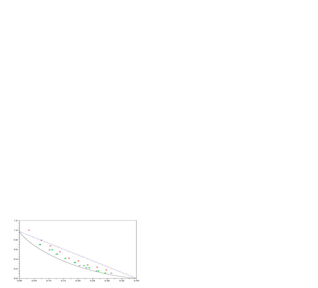
Rate-distortion performance. It is evident that the compression performance obtained by GVW and HYB is near-identical, and better than that of LLZ. This example was also examined by Rissanen and Tabus in [41], where it was noted that it is quite hard for any implementable scheme to produce rate-distortion pairs below the straight line connecting the end-points of the rate-distortion curve corresponding to and . As noted in [19], the Rissanen-Tabus scheme produces results slightly below the straight line, and it is one of the best implementable schemes for this problem.
| Bern(0.4) source, Hamming distortion | |||||
|---|---|---|---|---|---|
| Performance parameters | |||||
| Algorithm | rate | memory | time | ||
| HYB | 0.05 | 0.06952 | 0.70095 | 0.79MB | 2m45s |
| HYB | 0.08 | 0.11238 | 0.59143 | 0.6MB | 3m06s |
| HYB | 0.11 | 0.12952 | 0.50381 | 0.59MB | 3m33s |
| HYB | 0.14 | 0.15714 | 0.41619 | 0.56MB | 4m06s |
| HYB | 0.17 | 0.19143 | 0.32857 | 0.52MB | 4m40s |
| HYB | 0.2 | 0.22095 | 0.26286 | 0.53MB | 5m21s |
| HYB | 0.23 | 0.23905 | 0.21905 | 0.51MB | 5m26s |
| HYB | 0.26 | 0.27048 | 0.15333 | 0.53MB | 6m27s |
| HYB | 0.29 | 0.29333 | 0.10952 | 0.53MB | 6m56s |
Memory and complexity. Tables 1 and 2 contain a complete listing off all performance parameters obtained in the above experiment, including the execution time required for the encoder and the total amount of memory used. As already observed in Section 2, the LLZ scheme requires much less memory that GVW, and so does the hybrid algorithm HYB. In fact, while GVW and HYB produce essentially identical rate-distortion performance, the HYB algorithm requires between 32 and 213 times less memory than GVW. [Note that these figures are deterministic; the memory requirement is fixed by the description of the algorithm and it is not subject to random variations produced by the simulated data.] In terms of the corresponding execution times, the GVW and HYB share the exact same theoretical complexity in their implementation. Nevertheless, because of the vastly different memory requirements, in practice we find that the execution times of HYB were approximately three to ten times faster than GVW.
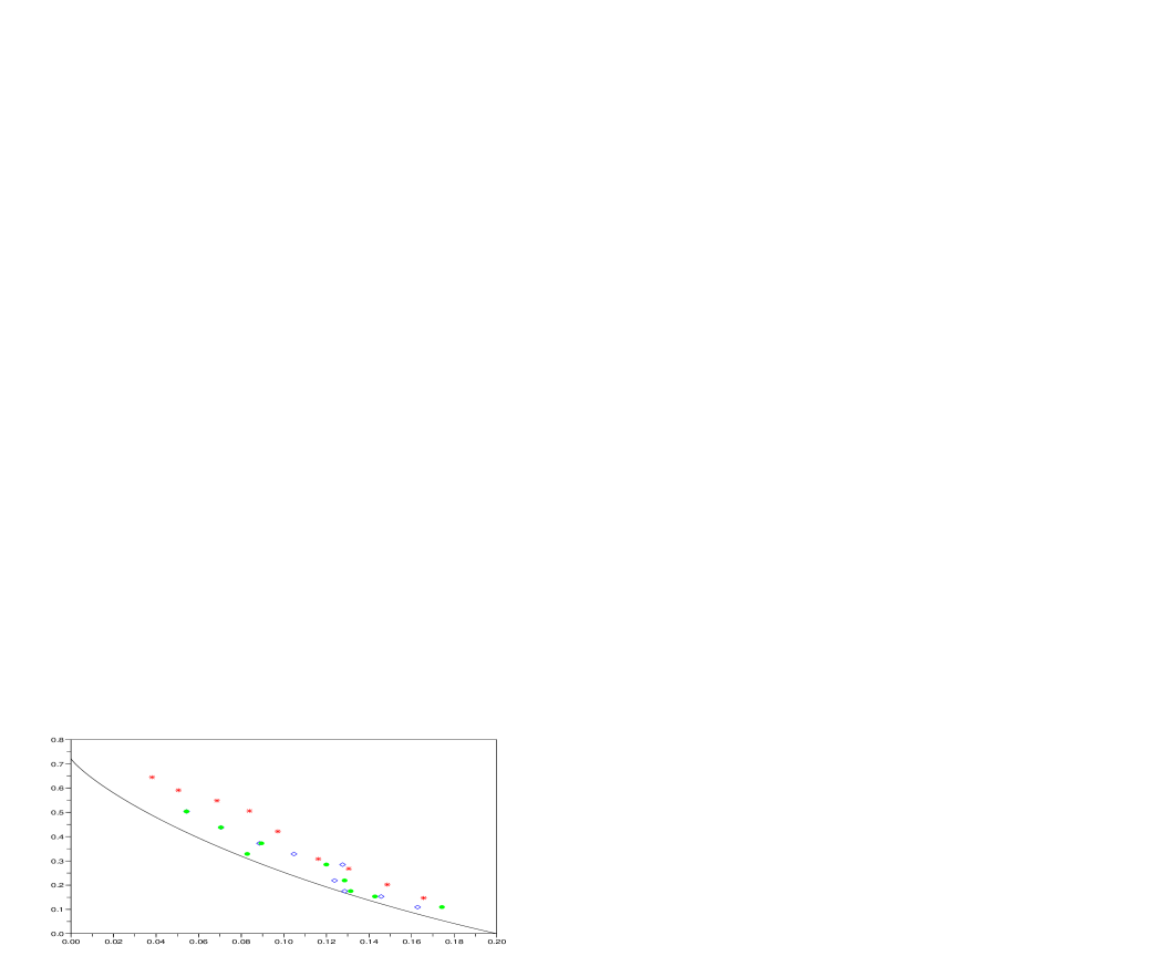
The second example is again on a Bernoulli source with respect to Hamming distortion, this time with source parameter . The corresponding simulation results are displayed in Figure 3 and Table 3.
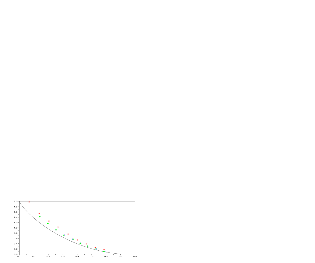
Finally, in the third example is taken as a memoryless source uniformly distributed on , to be compressed with respect to Hamming distortion. The empirical results are shown in Figure 4 and Table 4.
In both these cases, the same qualitative conclusions are drawn. The rate-distortion performance of the GVW and HYB algorithms is essentially indistinguishable, while the compression achieved by LLZ is generally somewhat worse, though in several instances not significantly so. In the second example note that the memory required by HYB is smaller than that of GVW by a factor that ranges between 44 and 242, while in the third example the corresponding factors are between 16 and 218. And again, although the theoretical implementation complexity of GVW and HYB is identical, because of their different memory requirements the encoding time of HYB is smaller than that of GVW by a factor ranging between approximately 3 and 9 in the second example, and between 1.25 and 1.5 in the third example.
| Bern(0.2) source, Hamming distortion | |||||
|---|---|---|---|---|---|
| Performance parameters | |||||
| Algorithm | rate | memory | time | ||
| GVW | 0.04 | 0.05429 | 0.50381 | 25MB | 19m05s |
| GVW | 0.055 | 0.07048 | 0.4381 | 28MB | 18m13s |
| GVW | 0.07 | 0.08857 | 0.37238 | 35MB | 19m50s |
| GVW | 0.085 | 0.10476 | 0.32857 | 42MB | 20m14s |
| GVW | 0.1 | 0.12762 | 0.28476 | 49MB | 19m55s |
| GVW | 0.115 | 0.12381 | 0.21905 | 59MB | 20m03s |
| GVW | 0.13 | 0.12857 | 0.17524 | 73MB | 19m57s |
| GVW | 0.145 | 0.14571 | 0.15333 | 90MB | 19m08s |
| GVW | 0.16 | 0.16286 | 0.10952 | 126MB | 19m38s |
| LLZ | 0.04 | 0.0381 | 0.64495 | 1.36MB | 3m05s |
| LLZ | 0.055 | 0.05048 | 0.59165 | 2.02MB | 7m45s |
| LLZ | 0.07 | 0.06857 | 0.54836 | 1.9MB | 8m02s |
| LLZ | 0.085 | 0.08381 | 0.50616 | 2.4MB | 13m38s |
| LLZ | 0.1 | 0.09714 | 0.42154 | 3.1MB | 22m18s |
| LLZ | 0.115 | 0.11619 | 0.3083 | 5.2MB | 24m03s |
| LLZ | 0.13 | 0.13048 | 0.26809 | 8.3MB | 58m07s |
| LLZ | 0.145 | 0.14857 | 0.20223 | 21MB | 132m30s |
| LLZ | 0.16 | 0.16571 | 0.1472 | 100MB | 377m10s |
| HYB | 0.04 | 0.05429 | 0.50381 | 0.56MB | 2m02s |
| HYB | 0.055 | 0.07048 | 0.4381 | 0.53MB | 2m54s |
| HYB | 0.07 | 0.08952 | 0.37238 | 0.57MB | 3m32s |
| HYB | 0.085 | 0.08286 | 0.32857 | 0.58MB | 3m52s |
| HYB | 0.1 | 0.12 | 0.28476 | 0.57MB | 4m46s |
| HYB | 0.115 | 0.12857 | 0.21905 | 0.56MB | 5m21s |
| HYB | 0.13 | 0.13143 | 0.17524 | 0.55MB | 5m45s |
| HYB | 0.145 | 0.14286 | 0.15333 | 0.52MB | 6m30s |
| HYB | 0.16 | 0.17429 | 0.10952 | 0.52MB | 7m11s |
| source, Hamming distortion | |||||
|---|---|---|---|---|---|
| Performance parameters | |||||
| Algorithm | rate | memory | time | ||
| GVW | 0.1 | 0.1419 | 1.41714 | 43MB | 10m27s |
| GVW | 0.16 | 0.20095 | 1.16095 | 24MB | 6m44s |
| GVW | 0.22 | 0.25238 | 0.92 | 31MB | 8m19s |
| GVW | 0.28 | 0.31333 | 0.72286 | 44MB | 11m12s |
| GVW | 0.34 | 0.36762 | 0.56952 | 43MB | 9m45s |
| GVW | 0.4 | 0.42381 | 0.41619 | 65MB | 12m29s |
| GVW | 0.46 | 0.47238 | 0.30667 | 92MB | 13m59s |
| GVW | 0.52 | 0.53238 | 0.19714 | 124MB | 14m12s |
| GVW | 0.58 | 0.58952 | 0.10952 | 229MB | 17m30s |
| LLZ | 0.1 | 0.06857 | 1.97778 | 3.597MB | 9m54s |
| LLZ | 0.16 | 0.1381 | 1.53794 | 1.79MB | 7m46s |
| LLZ | 0.22 | 0.20381 | 1.25461 | 2.04MB | 12m50s |
| LLZ | 0.28 | 0.26952 | 1.02841 | 2.61MB | 18m51s |
| LLZ | 0.34 | 0.33524 | 0.76228 | 3.445MB | 28m25s |
| LLZ | 0.4 | 0.4019 | 0.5393 | 3.49MB | 30m37s |
| LLZ | 0.46 | 0.46381 | 0.3893 | 5.44MB | 46m19s |
| LLZ | 0.52 | 0.52571 | 0.25807 | 14.6MB | 105m56s |
| LLZ | 0.58 | 0.58571 | 0.17475 | 104MB | 62m16s |
| HYB | 0.1 | 0.1419 | 1.41714 | 2.58MB | 7m49s |
| HYB | 0.16 | 0.19714 | 1.16095 | 1.22MB | 5m06s |
| HYB | 0.22 | 0.25429 | 0.92 | 1.26MB | 6m37s |
| HYB | 0.28 | 0.30762 | 0.72286 | 1.39MB | 8m48s |
| HYB | 0.34 | 0.37238 | 0.56952 | 1.05MB | 7m42s |
| HYB | 0.4 | 0.42095 | 0.41619 | 1.18MB | 9m39s |
| HYB | 0.46 | 0.47143 | 0.30667 | 1.15MB | 10m34s |
| HYB | 0.52 | 0.52952 | 0.19714 | 1.01MB | 10m14s |
| HYB | 0.58 | 0.58476 | 0.10952 | 1.05MB | 11m43s |
5 Conclusions and Extensions
The starting point for this work was the observation that there is a certain duality relationship between the divide-and-conquer compression schemes of Gupta-Verdú-Weissman (GVW) in [19], and certain lossy Lempel-Ziv schemes based on a fixed-database as in [24]. To explore this duality, LLZ, a new (non-universal) lossy LZ algorithm was introduced, and it was shown to be asymptotically rate-distortion optimal. To combine the low-complexity advantage of GVW with the low-memory requirement of LLZ, a hybrid algorithm, called HYB, was then proposed, and its properties were explored both theoretically and empirically.
The main contribution of this short paper is the introduction of memory considerations in the usual compression-complexity trade-off. Building on the success of the GVW algorithm, it was shown that the HYB scheme simultaneously achieves three goals: 1. Its rate-distortion performance can be made arbitrarily close to the fundamental rate-distortion limit; 2. The encoding complexity can be tuned in a rigorous manner so as to balance the trade-off of encoding complexity vs. compression redundancy; and 3. The memory required for the execution of the algorithm is much smaller than that required by GVW, a difference which may be made arbitrarily large depending on the choice of parameters.
Moreover, empirically, for blocklengths of the order of thousands, the HYB scheme appears to outperform existing schemes for the compression of simple memoryless sources with respect to Hamming distortion.
Lastly, we briefly mention that the results presented in this paper can be extended in several directions. First we note that the finite-alphabet assumption was made exclusively for the sake of simplicity of exposition and to avoid cumbersome technicalities. While keeping the structure of all three algorithms exactly the same, this assumption can easily be relaxed, at the price of longer, more technical proofs, along the lines of arguments, e.g., in [49][24][25][19]. For example, Theorem 4 of [19] which gives precise performance and complexity bounds for the GVW used with general source and reproduction alphabets and with respect to an unbounded distortion measure, can easily be generalized to HYB. Similarly, Theorem 5 of [19] which describes the performance of a universal version of GVW can also be generalized to the corresponding statement for a universal version of HYB (with obvious modifications), although, as noted in [19], the utility of that result is purely of theoretical interest.
Appendix
Proof of Theorem 1.
Recall that, under the present assumptions, the rate-distortion function is continuous, differentiable, convex and nonincreasing [6][12]. Given and , assume without loss of generality that ; then we can choose according to , so that . [As it does not change the asymptotic analysis below, we take fixed and arbitrary.] Then the distortion part of the theorem is immediate by the construction of the algorithm.
Before considering the rate, we record two useful asymptotic results for the match-lengths . Let , and as in (3). Then [14, Theorem 23] immediately implies that,
Moreover, for any , the following more precise asymptotic lower bound on holds: As ,
| (9) |
The proof of (9) is a straightforward simplification of the proof of [24, Corollary 3], and therefore omitted.
Now let arbitrary. The encoder parses the message into distinct words , each of length . We let and following [48] we assume, without loss of generality, that is an integer and that the last phrase is complete, i.e.,
To bound above the rate obtained by LLZ, we consider phrases of different lengths separately. We call a phrase long if its length satisfies , and we call short otherwise. Recalling (6), the total description length of the LLZ can be broken into two parts as,
| (10) | |||||
For the first sum we note that, by the choice of and the definition of a short phrase, each summand is bounded above by a constant times , at least for all large enough; therefore, the conditional expectation of the whole sum given is bounded by,
where denotes the indicator function of an event , and the inequality follows by considering not just all ’s, but all the possible positions in where a short match can occur. Dividing by and letting , from (9) we get that this expression converges to zero w.p. 1, so that the conditional expectation of the first term in (10) also converges to zero, w.p.1.
For the second and dominant term in (10), let be the number of long phrases . Since each long has length , we must have , so that
| (11) |
Also, by the definition of , for all large enough (independently of ), we have,
Therefore, the second sum in (10) can be bounded above by,
Combining this with the fact that the first term in (10) vanishes, immediately yields
and since was arbitrary we get the first claim in the theorem. Finally, the second claim follows from the first and Fatou’s lemma.
Proof of Theorem 2.
The proof of the theorem is based on Lemma 1 below, which plays the same role as [19, Lemma 1] in the proof of [19, Theorem 1]. The rest of of the proof is identical, except for the fact that we do not need to invoke the law of large numbers, since here we do not claim that the probability of excess distortion goes to zero.
Before stating the lemma, we define the following auxiliary quantities: , ,
and,
Lemma 1. Consider a memoryless source to be compressed at target distortion level . Then for any , the HYB algorithm with parameters and
| (12) |
when applied to a single block achieves rate , and its expected distortion is less than .
Proof. Given , choose a positive such that,
Now follow the proof of [19, Lemma 1] with in place of , until the beginning of the computation of the probability of excess distortion. The key observation is that, for HYB, this probability can be bounded above by the excess-distortion probability with respect to a random codebook with
words, by just considering possible matches starting at positions , making the corresponding potentially matching blocks in the database independent. Therefore, following the same computation, the required probability can be bounded above as before by,
| (13) |
The first term is bounded above by,
as before, and in order to show that the expected distortion is less than it suffices to show that the last term satisfies,
| (14) |
Substituting the choice of from (12), it becomes,
and since is restricted to be less than one, this can in turn be bounded above, uniformly in , by its value at . [To see that, note that the function is increasing for and decreasing for . By our choice of , the maximum above is achieved at the point .] Therefore, noting also that , this term is bounded above by,
which, after some algebra, simplifies to,
and this is less than by the choice of . This establishes (14) and completes the proof of the lemma.
Proof of Theorem 3.
Taking arbitrary, we let, as in the proof of [19, Theorem 3],
For each we use HYB with the corresponding parameters; the rate result follows from the construction of the algorithm, which, at blocklength , has rate no larger than,
as .
Regarding the distortion, equation (13) in the proof of Theorem 2 shows that that the probability of the event that the distortion of the th block will exceed is bounded above by,
It is easily seen that, for large , this is dominated by the second term,
Therefore, the distortion of any one -block is bounded above by,
Noting that the excess term goes to zero as , it will still go to zero when averaged out over all sub-blocks, and, therefore, the expected distortion over the whole message will converge to .
Finally, the complexity results are straightforward by construction; see the discussion in [19, Section II-A].
Acknowledgments
References
- [1] M. Alzina, W. Szpankowski, and A. Grama. 2D-pattern matching image and video compression. IEEE Trans. Image Processing, 11:318–331, 2002.
- [2] D. Arnaud and W. Szpankowski. Pattern matching image compression with prediction loop: Preliminary experimental results. In Proc. Data Compression Conf. – DCC 97, Los Alamitos, California, 1997. IEEE, IEEE Computer Society Press.
- [3] M. Atallah, Y. Génin, and W. Szpankowski. Pattern matching image compression: Algorithmic and empirical results. IEEE Trans. Pattern Analysis and Machine Intelligence, 21:618–627, 1999.
- [4] M. Atallah, Y. Génin, and W. Szpankowski. Pattern matching image compression: Algorithmic and empirical results. IEEE Trans. Pattern Analysis and Machine Intelligence, 21, 1999.
- [5] J.G. Bell, T.C. Cleary and I.H. Witten. Text Compression. Prentice Hall, New Jersey, 1990.
- [6] T. Berger. Rate Distortion Theory: A Mathematical Basis for Data Compression. Prentice-Hall Inc., Englewood Cliffs, NJ, 1971.
- [7] P.A. Chou, M. Effros, and R.M. Gray. A vector quantization approach to universal noiseless coding and quantizations. IEEE Trans. Inform. Theory, 42(4):1109–1138, 1996.
- [8] S. Ciliberti, M. Mézard, and R. Zecchina. Message-passing algorithms for non-linear nodes and data compression. ComPlexUs, 3:58–65, 2006.
- [9] T.M. Cover and J.A. Thomas. Elements of Information Theory. J. Wiley, New York, 1991.
- [10] M. Crochemore and T. Lecroq. Pattern-matching and text-compression algorithms. ACM Computing Surveys, 28(1):39–41, 1996.
- [11] M. Crochemore and W. Rytter. Text Algorithms. Oxford University Press, New York, 1994.
- [12] I. Csiszár and J. Körner. Information Theory: Coding Theorems for Discrete Memoryless Systems. Academic Press, New York, 1981.
- [13] A. Dembo and I. Kontoyiannis. The asymptotics of waiting times between stationary processes, allowing distortion. Ann. Appl. Probab., 9:413–429, 1999.
- [14] A. Dembo and I. Kontoyiannis. Source coding, large deviations, and approximate pattern matching. IEEE Trans. Inform. Theory, 48:1590–1615, June 2002.
- [15] B.J. Frey. Graphical Models for Machine Learning and Digital Communication. MIT Press, Cambridge, MA, USA, 1998.
- [16] A. Gersho and R.M. Gray. Vector Quantization and Signal Compression. Kluwer Academic Publishers, Boston, 1992.
- [17] R.M. Gray and D.L. Neuhoff. Quantization. IEEE Trans. Inform. Theory, 44(6):2325–2383, 1998.
- [18] A. Gupta and S. Verdú. Nonlinear sparse-graph codes for lossy compression. Preprint, 2008.
- [19] A. Gupta, S. Verdú, and T. Weissman. Rate-distortion in near-linear time. Preprint, 2008.
- [20] D. Hankerson, G.A. Harris, and P.D. Johnson, Jr. Introduction to Information Theory and Data Compression. CRC Press LLC, 1998.
- [21] S. Jalali, A. Montanari, and T. Weissman. An implementable scheme for universal lossy compression of discrete Markov sources. Preprint, 2008.
- [22] S. Jalali and T. Weissman. Rate-distortion via Markov chain Monte Carlo. In Proc. of the IEEE International Symposium on Inform. Theory, pages 852–856, Toronto, Canada, July 2008.
- [23] J.C. Kieffer. A survey of the theory of source coding with a fidelity criterion. IEEE Trans. Inform. Theory, 39(5):1473–1490, 1993.
- [24] I. Kontoyiannis. An implementable lossy version of the Lempel-Ziv algorithm – Part I: Optimality for memoryless sources. IEEE Trans. Inform. Theory, 45(7):2293–2305, November 1999.
- [25] I. Kontoyiannis. Pointwise redundancy in lossy data compression and universal lossy data compression. IEEE Trans. Inform. Theory, 46(1):136–152, January 2000.
- [26] Jr. Langdon, G.G. An introduction to arithmetic coding. IBM J. Res. Develop., 28(2):135–149, 1984.
- [27] T. Linder, G. Lugosi, and K. Zeger. Rates of convergence in the source coding theorem, in empirical quantizer design, and in universal lossy source coding. IEEE Trans. Inform. Theory, 40(6):1728–1740, 1994.
- [28] T. Łuczak and W. Szpankowski. A suboptimal lossy data compression algorithm based on approximate pattern matching. IEEE Trans. Inform. Theory, 43(5):1439–1451, 1997.
- [29] D.J.C. MacKay. Information Theory, Inference and Learning Algorithms. Cambridge University Press, New York, 2003.
- [30] D.J.C. Mackay and R.M. Neal. Good codes based on very sparse matrices. In Cryptography and Coding. 5th IMA Conference, number 1025 in Lecture Notes in Computer Science, pages 100–111. Springer, 1995.
- [31] Y. Mao and A. Banihashemi. Design of good LDPC codes using girth distribution. In Int. Symp. Inform. Theory, Sorrento, Italy, 2000.
- [32] E. Martinian and M. Wainwright. Low density codes achieve the rate-distortion bound. In Proc. Data Compression Conf. – DCC 2006, pages 153–162, Snowbird, UT, March 2006.
- [33] Y. Matsunaga and H. Yamamoto. A coding theorem for lossy data compression by LDPC codes. IEEE Trans. Inform. Theory, 49(9):2225–2229, Sept. 2003.
- [34] S. Miyake. Lossy data compression over Zq by LDPC code. In Proc. of the IEEE International Symposium on Inform. Theory, page 813, Seattle, WA, July 2006.
- [35] H. Morita and K. Kobayashi. An extension of LZW coding algorithm to source coding subject to a fidelity criterion. In 4th Joint Swedish-Soviet Int. Workshop on Inform. Theory, pages 105–109, Gotland, Sweden, 1989.
- [36] J. Muramatsu and F. Kanaya. Distortion-complexity and rate-distortion function. IEICE Trans. Fundamentals, E77-A:1224–1229, 1994.
- [37] R.M. Neuhoff, D.L. Gray and L.D. Davisson. Fixed rate universal block source coding with a fidelity criterion. IEEE Trans. Inform. Theory, 21(5):511–523, 1975.
- [38] D. Ornstein and P.C. Shields. Universal almost sure data compression. Ann. Probab., 18:441–452, 1990.
- [39] R.C. Pasco. Source Coding Algorithms for Fast Data Compression. PhD thesis, Dept. of Electrical Engineering, Stanford, CA, USA, 1976.
- [40] T. Richardson and R. Urbanke. Modern Coding Theory. Cambridge University Press, Cambridge, UK, 2008.
- [41] J. Rissanen and I. Tabus. Rate-distortion without random codebooks. In Workshop on Information Theory and Applications (ITA), UCSD, San Diego, CA, January 2006.
- [42] J.J. Rissanen. Generalized Kraft inequality and arithmetic coding. IBM J. Res. Develop., 20(3):198–203, 1976.
- [43] C.E. Shannon. Coding theorems for a discrete source with a fidelity criterion. IRE Nat. Conv. Rec., part 4:142–163, 1959. Reprinted in D. Slepian (ed.), Key Papers in the Development of Information Theory, IEEE Press, 1974.
- [44] M. Sipser and D.A. Spielman. Expander codes. IEEE Trans. Inform. Theory, 42:1710–1722, 1996.
- [45] Y. Steinberg and M. Gutman. An algorithm for source coding subject to a fidelity criterion, based upon string matching. IEEE Trans. Inform. Theory, 39(3):877–886, 1993.
- [46] M.J. Wainwright and E. Maneva. Lossy source encoding via message-passing and decimation over generalized codewords of LDGM codes. In Proc. of the IEEE International Symposium on Inform. Theory, pages 1493–1497, Adelaide, Australia, Sept. 2005.
- [47] N. Wiberg, H.-A. Loeliger, and R. Koetter. Codes and iterative decoding on general graphs. European Transactions in Telecommunication, 6:513–525, 1995.
- [48] A.D. Wyner and J. Ziv. Fixed data base version of the Lempel-Ziv data compression algorithm. IEEE Trans. Inform. Theory, 37(3):878–880, 1991.
- [49] E.-H. Yang and J.C. Kieffer. Simple universal lossy data data compression schemes derived from the Lempel-Ziv algorithm. IEEE Trans. Inform. Theory, 42(1):239–245, 1996.
- [50] E.-H. Yang and J.C. Kieffer. On the performance of data compression algorithms based upon string matching. IEEE Trans. Inform. Theory, 44(1):47–65, 1998.
- [51] E.-H. Yang, Z. Zhang, and T. Berger. Fixed-slope universal lossy data compression. IEEE Trans. Inform. Theory, 43(5):1465–1476, 1997.
- [52] R. Zamir and K. Rose. Natural type selection in adaptive lossy compression. IEEE Trans. Inform. Theory, 47(1):99–111, 2001.
- [53] Z. Zhang and V.K. Wei. An on-line universal lossy data compression algorithm by continuous codebook refinement – Part I: Basic results. IEEE Trans. Inform. Theory, 42(3):803–821, 1996.
- [54] Z. Zhang and E.-H. Yang. An on-line universal lossy data compression algorithm by continuous codebook refinement – Part II: Optimality for phi-mixing models. IEEE Trans. Inform. Theory, 42(3):822–836, 1996.
- [55] J. Ziv. Coding of sources with unknown statistics – Part II: Distortion relative to a fidelity criterion. IEEE Trans. Inform. Theory, 18(3):389–394, 1972.
- [56] J. Ziv. Coding theorems for individual sequences. IEEE Trans. Inform. Theory, 24(4):405–412, 1978.
- [57] J. Ziv. Distortion-rate theory for individual sequences. IEEE Trans. Inform. Theory, 26(2):137–143, 1980.
- [58] J. Ziv and A. Lempel. A universal algorithm for sequential data compression. IEEE Trans. Inform. Theory, 23(3):337–343, 1977.
- [59] J. Ziv and A. Lempel. Compression of individual sequences by variable rate coding. IEEE Trans. Inform. Theory, 24(5):530–536, 1978.