Lost in the Shuffle: Testing Power in the Presence of Errorful Network Vertex Labels
Abstract
Two-sample network hypothesis testing is an important inference task with applications across diverse fields such as medicine, neuroscience, and sociology. Many of these testing methodologies operate under the implicit assumption that the vertex correspondence across networks is a priori known. This assumption is often untrue, and the power of the subsequent test can degrade when there are misaligned/label-shuffled vertices across networks. This power loss due to shuffling is theoretically explored in the context of random dot product and stochastic block model networks for a pair of hypothesis tests based on Frobenius norm differences between estimated edge probability matrices or between adjacency matrices. The loss in testing power is further reinforced by numerous simulations and experiments, both in the stochastic block model and in the random dot product graph model, where the power loss across multiple recently proposed tests in the literature is considered. Lastly, the impact that shuffling can have in real-data testing is demonstrated in a pair of examples from neuroscience and from social network analysis.
1 Introduction
Interest in graph and network-valued data has soared in the last decades [1], as networks have become a common data type for modeling complex dependencies and interactions in many fields of study, ranging from neuroscience [2, 3, 4] to sociology [5, 6] to biochemistry [7, 8], among others. As network data has become more commonplace, a number of statistical tools tailored for handling network data have been developed [9, 10], including methods for hypothesis testing [11, 12, 13], goodness-of-fit analysis [14, 15, 16], clustering [17, 18, 19, 20, 21, 22], and classification [23, 24, 25, 26], among others.
While early work on network inference often considered a single network as the data set, there has been a relatively recent proliferation of datasets that consist of multiple networks on the same set of vertices (which we will referred to as the “paired” setting) and multiple networks on differing vertex sets (the “unpaired” setting). In the paired setting, example datasets include the DTMRI and FMRI connectome networks considered in [11, 27, 28], and the paired social networks from Twitter (now X) in [29] and from Facebook [30, 31] to name a few. In the unpaired setting, example datasets include the social networks that partially share a user base from [32, 33] and the friendship networks in [34]. When considering multiple paired networks for a single inference task, these methods often make an implicit assumption that the graphs are “vertex-aligned,” i.e., that there is an a priori known, true, one–to–one correspondence across the vertex labels of the graphs. Often, this is not the case in practice (see the voluminous literature on network alignment and graph matching [35, 36, 37]), as node alignments may be obscured by numerous factors, including, for example, different usernames across social networks [33], unknown correspondence of neurons across brain hemispheres [38], and misalignments/misregistrations to a common brain atlas (to create connectomes) as discussed in [39]. Moreover, these errors across the observed vertex labels can have a dramatically detrimental impact on subsequent inferential performance [40].
An important inference task in the multiple network setting is two-sample network hypothesis testing [41, 42]. Two-sample network testing has been used, for example, to compare neurological properties (captured via patient connectomes) of populations of patients along various demographic characteristics like age, sex, and the presence/absence of a neurological disorder (indeed, this connectomic testing example will serve as motivation for us in Section 1.3). Among the work in this area, numerous methods exist for (semi)parametric hypothesis testing across network samples, where one of the parameters being leveraged is the correspondence of labels across networks; see for example [11, 43, 44, 45]. There are also nonparametric methods that estimate and compare network distributions, and ignore the information contained in the vertex labels; see, for example, [12, 46].
This paper considers an amalgam of the above settings in which there is signal to be leveraged in one portion of the vertex labels, and uncertainty across the remaining labels. Our principle task is then two-fold. First, we seek to understand how this label uncertainty impacts testing power both theoretically (Section 2) and in practice (Sections 3–5). Second, we seek to better understand how to mitigate the impact of this uncertainty via a graph matching preprocessing step that aligns the graphs before testing (Section 6). Before formally defining the shuffled testing problem, we will first set here some of the notational conventions that will appear throughout the paper. Note also that all necessary code to reproduce the figures in the paper can be found at https://www.math.umd.edu/~vlyzinsk/Shuffled_testing/.
1.1 Notation
Given an undirected graph -vertex graph (all graphs considered will be undirected graphs with no self-loops), we let denote the vertices of . The adjacency matrix A of is given by: for all . We note here that we will refer to a graph and its adjacency matrix interchangeably, as these objects (in the setting we consider herein) encode equivalent information. We denote the row of any matrix M with the notation (or via if the subscript is needed to denote explicit dependence on ).
We define the usual Frobenius norm of a matrix A via
For positive integers and , we will define the set of orthogonal matrices in via and the set of permutation matrices via . We indicate a matrix of all ones of size by , and is the matrix of all one of size . Similarly, we denote the corresponding matrices of all 0’s by and Lastly, the direct sum of two matrices A and B is denoted by .
For functions , we use here the standard asymptotic notations:
Note that when (resp., and ) when is a complicated function of , we will often write (resp., and ) to ease notation.
1.2 Shuffled testing
To formalize our partially aligned graph setting, suppose we have two networks and on a common vertex set , and that the label correspondence across networks is known for of the vertices; denote the set of these vertices via . We further assume that the user has knowledge of which vertices are in . This, for example, could be the result of graph matching algorithms that provide a measure of certainty for the validity of each matched vertex (see, for example, the soft matching approach of [47] or the vertex nomination work of [48, 49]). The veracity of the correspondence across the remaining vertices not in (which we shall denote via ), is assumed unknown a priori. This may be due, for example, to algorithmic uncertainty in aligning nodes across networks or noise in the data. We then have that there exists an unknown (where is the set of permutation matrices)
such that the practitioner observes and . Given the above framework, it is natural to consider the following semiparametric adaptation of the traditional parametric tests. From and , the user seeks to test if the distribution of is different than from that of , i.e., to test the following hypotheses (where denotes the distribution (law) of ), versus In this work, we will be considering testing within the family of (conditionally) edge-independent graph models, so that is completely determined by . Focusing our attention first on a simple Frobenius-norm based hypothesis test (later considering the spectral embedding based tests of [45, 11, 12]), we reject if
is suitably large; here is an estimate of obtained from , and an estimate of (this will be formalized later in Section 1.5; for intuition and experimental validation on why the test statistic using is preferable to the adjacency-based test using as its statistic, see Section 3). To account for the uncertainty in the labeling of , for each and , define to be the smallest value such that
As we do not know which element of yields the shuffling from to , a valid (conservative) level- test using the Frobenius norm test statistic would reject if
The price of this validity is a loss in testing power against any fixed alternative, especially in the scenario where (the true, but unknown, shuffling) shuffles fewer than vertices in . In this case the conservative test is over-correcting for the uncertainty in . The question we seek to answer is how much testing power is lost in this shuffle, and how robust the adaptations of different testing methods (i.e., different test statistics) are to this shuffling.
1.3 Motivating example: DTMRI connectome testing
To motivate the shuffled testing problem further, we first present the following real-data example. We consider the test/retest connectomic dataset from [52] processed via the algorithmic pipeline at [53] (note that this data is available for download at http://www.cis.jhu.edu/~parky/Microsoft/JHU-MSR/ZMx2/BNU1/DS01216-xyz.zip). This dataset represents human connectomes derived from DTMRI scans, where there are multiple (i.e., test/retest) scans per each of the 57 individuals in the study. We consider three such scans, yielding connectomes and and . Here, and represent test/retest scans from one subject (subject 1) and a scan from a different subject (subject 2 scan 1). In each scan, vertices represent voxel regions of the brain with edges denoting whether a neuronal fiber bundle connects the two regions or not (so that the graphs are binary and undirected). Considering only vertices common to the three connectomes, we are left with three graphs each with vertices.
For , let be an unknown permutation. Observing and and (rather than and ) we seek to test whether is a connectome drawn from the same person as and or from a different person (i.e., under the reasonable assumption that , we seek to test whether is from this same distribution). Ideally, we would then construct our test statistic as
| (1) |
where is the estimate of or derived from as in Section 1.5.
Incorporating the unknown shuffling of in is tricky here, as for moderate it is computationally infeasible to compute for all (where we recall that is the smallest value such that indeed, the order of is given we know the vertices in ), and so it is difficult to compute the conservative critical value . Here, the task of finding the worse-case shuffling in can be cast as finding an optimal matching between one graph and the complement of the second, which we suspect is computationally intractable. To proceed forward, then, we consider the following modification of the overall testing regime: We consider a fixed (randomly chosen) sequence of nested permutations for and consider shuffling by and by for all . We then repeat this process times, each time obtaining an estimate (via bootstrapping as outlined below) of testing power against . This is done here out of computational necessity, and although the test does not achieve level- here, this will nonetheless be sufficient to demonstrate the dramatic loss in testing performance due to shuffling.
In order to estimate the testing power here, we rely on the bootstrapping heuristic inspired by [45, 51] for latent position networks. Informally, we will model , , and as instantiations of the Random Dot Product Graph (RDPG) modeling framework of [54].
Definition 1.1.
Let be such that for all . We say that is an instance of a d-dimensional Random Dot Product Graph (RDPG) with latent positions X and sparsity parameter if given X, the entries of the random, symmetric, hollow adjacency matrix satisfy for all ,
In this framework (where we here have , we posit matrices of latent positions , for , , and for (with ), such that the -th row of X, (resp., Y) corresponds to the latent feature vector associated with the -th vertex in and (resp., ). In this setting, the distribution of networks from the same person (i.e., and ) will serve as our null distribution, and we seek to test , where .
The RDPG model posits a tractable parameterization of the networks provided by the latent position matrices, and there are a number of statistically consistent methods for estimating these parameters under a variety of model variants. Here, we will use the Adjacency Spectral Embedding (ASE) to estimate X and Y; see [55] for a survey of recent work in estimating and inference in RDPGs.
Definition 1.2.
(Adjacency Spectral Embedding) Given the adjacency matrix of an -vertex graph, the Adjacency Spectral Embedding (ASE) of A into is given by
| (2) |
where is the spectral decomposition of is the diagonal matrix with the ordered largest singular values of A on its diagonal, and is the matrix whose columns are the corresponding orthonormal eigenvectors of A.
Once suitable estimates of the parameters are obtained—denoted for those derived via ASE of respectively, and derived via ASE of —we use a parametric bootstrap (here with 200 bootstrap samples) to estimate the null distribution critical value of where in the -th bootstrap sample, the test statistic
is computed as follows: For each ,
-
(i)
sample independent RDPG;
-
(ii)
compute ASE();
-
(iii)
set .
Note that we use a single embedding dimension for all the ASE’s in the null, estimated as detailed in Remark 1.3. Given this estimated critical value, we then estimate the testing level and testing power as follows. For each , we mimic the above procedure (again with 200 bootstrap samples) to estimate the distributions of and where (resp., ) is the ASE derived estimate of (resp., ); note that similar bootstrapping procedures were considered in [11, 45]. The estimated testing level (resp., power) under the null hypothesis that (resp., under the alternative that ) is then computed by calculating the proportion of (resp., ) greater than the estimated critical value.
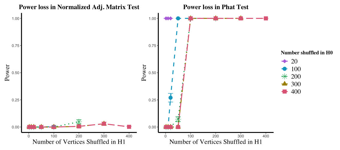
Estimated power for 200 bootstrapped samples of these test statistics at approximate level are plotted in Figure 1 left panel (averaged over the Monte Carlo replicates). In the figure, the -axis represents the number of vertices shuffled via (from to ) while the curve colors represent the maximum number of vertices potentially shuffled via ; here all shuffled by . As seen in figure, the power of this test increases as both and increase, implying that the test is able to correctly distinguish the difference between the two subjects when the effect of the shuffling is either minimal (small ) or when the shuffling is equally severe in both the null and alternative cases (i.e., shuffles as much as ). When is much bigger than , the test is overly conservative (see Figure 1 right panel), as expected. In this case the shuffling in has the effect of inflating the critical value compared to the true (i.e., unshuffled) testing critical value, yielding an overly conservative test that cannot distinguish between the different test subjects.
1.4 Random graph models
As referenced above, to tackle the question of power loss statistically, we will anchor our analysis in commonly studied random graph models from the literature. In addition to the Random Dot Product Graph (RDPG) model [56, 54] mentioned above, we will also consider the Stochastic Blockmodel (SBM) [57] as a data generating mechanism. These models provide tractable settings for the analysis of graphs where the connectivity is driven by latent features—community membership in the SBM and the latent position vector in the RDPG.
The Stochastic Blockmodel—and its myriad variants including mixed membership [58], degree corrected [59], and hierarchical SBMs [25, 60]—provide a simple framework for networks with latent community structure.
Definition 1.3.
We say that an -vertex random graph SBM is distributed according to a stochastic block model random graph with parameters the number of blocks in graph, the block probability matrix, the block membership function, and the sparsity parameter, if
-
i.
The vertex set is partitioned into blocks where for each , we have denotes the size of the block (so that );
-
ii.
The block membership function is such that iff , and we have for each ,
Note that the block membership vector in an SBM is often modeled as a random multinomial vector with block probability parameter giving the probabilities of assigning vertices randomly to each of the blocks. Our analysis is done in the fixed block membership setting, although it translates immediately to the random membership setting. Note also that we will often be considering cases where the number of vertices in satisfies . In this case, we write so that the model parameters may vary in . However, to ease notation, we will suppress the subscript throughout, although the dependence on is implicitly understood.
In SBMs, the connectivity structure is driven by the latent community membership of the vertices. In the space of latent feature models, a natural extension of this idea is to have connectivity modeled as a function of more nuanced, vertex-level, features. In this direction, we will also consider framing our inference in the popular Random Dot Product Graph model introduced in Definition 1.1. Note that the RDPG model encompasses SBM models with positive semidefinite . Indefinite and negative definite SBM’s, are encompassed via the generalized RDPG [61], though the ordinary RDPG will be sufficient for our present purposes. Note also that our theory will be presented for the fixed latent position RDPG above, though it translates immediately to the random latent position setting (i.e., where the rows of , namely the , are i.i.d. from an appropriate distribution ).
Remark 1.1.
An inherent non-identifiability of the RDPG model comes from the fact that for any orthogonal matrix , we get . With this caveat, RDPGs are more suitable for modeling in inference tasks that are rotation invariant, such as clustering [21, 20], classification [24], and appropriately defined hypothesis testing settings [11, 45].
Remark 1.2.
If the RDPG graphs are directed or weighted, then appropriate modifications to the ASE are required to embed the networks (see, for example, [62] and [63]). Analogous concentration results are available in both settings, and we suspect that we can derive theory analogous to Theorems 2.1–2.2. Herein, we restrict ourselves to the unweighted RDPG, and leave the necessary modification to handle directed and weighted graph to future work.
As in [43], we will choose to control the sparsity of our graphs via and not through the latent position matrix or block probability matrix . As such, we will implicitly make the following assumption throughout the remainder for all RDPGs and positive semidefinite SBMs (when viewed as RDPGs):
Assumption 1.
If we consider a random graph sequence where , then we will assume that for all sufficiently large, we have that:
-
i.
is rank , and if are the singular values of , we have ;
-
ii.
There exists a fixed compact set such that the rows of are in for all ;
-
iii.
There exists a fixed constant such that entry-wise.
1.5 Model estimation
In the RDPG (and positive semidefinite SBM) setting, our initial hypothesis test will be predicated upon having a suitable estimate of . In this setting, the Adjacency Spectral Embedding (ASE) (see Definition 1.2) of [21] has proven to be practically useful and theoretically tractable means for obtaining such an estimate. The adjacency spectral embedding has a rich, recent history in the literature (see [55]) as a tool for estimating tractable graph representations, achieving its greatest estimation strength in the class of latent position networks (the RDPG being one such example). In these settings, it is often assumed that the rank of the latent position matrix X is , and that is considerably smaller than , the number of vertices in the graph.
A great amount of inference in the RDPG setting is predicated upon being a suitably accurate estimate of X. To this end, the key statistical properties of consistency and asymptotic residual normality are established for the ASE in [21, 64, 61] and [65, 55] respectively. These results (and analogues for unscaled variants of the ASE) have laid the groundwork for myriad subsequent inference results, including clustering [21, 64, 22, 66], classification [24], time-series analysis [41, 67], and vertex nomination [49, 68], among others.
Remark 1.3.
In practice, there are a number of heuristics for estimating the unknown embedding dimension in the ASE (see, for example, the work in [69, 70, 71]). In the real data experiments below, we will adopt an automated elbow-finder applied to the SCREE plot (as motivated by [72] and [70]); for the simulation experiments, we use the true value for the underlying RDPG’s/SBM’s. Estimating the correct dimension is of paramount importance in spectral graph inference, as underestimating introduces bias into the embedding estimate and overestimating introduces additional variance into the estimate. In our experience, underestimation of would have a more dramatic impact on subsequent inferential performance.
2 Shuffled graph testing in theory
In complicated testing regimes (e.g., the embedding-based tests of [11, 45, 44]), analyzing the distribution of the test under the alternative is itself a challenging proposition (see, for example, the work in [73, 11]). Accounting for a second layer of uncertainty due to the shuffling adds further complexity to the analysis. In order to build intuition for these more complex settings in the context of the RDPG and SBM models (which we will explore empirically in Section 4), we examine the effect on testing power of shuffling in the simple Frobenius norm test considered in Section 1.3.
We consider first the case where RDPG and we have an independent RDPG. Under the null , and we will consider elements of the alternative that satisfy the following: for all but rows of , we have so that we have where (with the proper vertex reordering)
| (3) |
We will further assume that there exists constants and such that for all entries of and . We note that we will assume throughout that both and satisfy the conditions of Assumption 1.
The principle challenge of testing in this regime is that the veracity of the (across graph) labels of vertices in is unknown a priori. It could be the case that these vertices were all shuffled or all correctly aligned, and it is difficult to disentangle the effect on testing power of versus the potential shuffling. To model this, we consider shuffled elements of the alternative, so that we observe and , where the true but unknown shuffling of is , which shuffles labels in .
2.1 Power analysis and the effect of shuffling: test
In this section, we will present a trio of theorems, namely Theorems 2.1–2.3, in which we characterize the impact on power of the two distinct sources of noise here: the shuffling error ( and ) and the error in the alternative captured here by . When the difference between and is comparably large (for example, when and ), then the power of the resulting test will be low even in the presence of modest error . In this case, the relative size of the error in the alternative is overwhelmed by the excess shuffling in the null which is needed to maintain testing level . The actual shuffling error (i.e., ) is much less than the conservative null shuffling (i.e., ), and the test is not able to distinguish the two graphs in light of the conservative test’s overcompensation. Even in the case where is relatively small, if the error is sufficiently small, we will have low testing power, as expected. However, when the difference between and is relatively small compared to , or and are both relatively small compared to (see the conditions in Theorem 2.1 and Theorem 2.2), then the difference in the number of vertices being shuffled across the conservative null and truly shuffled in the alternative is overwhelmed by the error in the alternative. In this case, the noise created by the relatively small differences in shuffling between null and alternative can be overcome, and high power can still be achieved.
2.1.1 Small regime
Before presenting the trio of theorems, we will first establish the following notation
-
i.
For let be the ASE-based estimate of derived from ;
-
ii.
For and for any , let be the ASE-based estimate of derived from ;
-
iii.
Let ; let be the shuffling of vertices in such that we observe .
In this section, we will be concerned with conditions under which power is asymptotically almost surely 1; specifically conditions under which the following holds for all sufficiently large
| (4) |
Our first result tackles the case in which is relatively small, and only modest error is needed to achieve high testing power. Note that the proof of Theorem 2.1 can be found in Appendix A.1.
Theorem 2.1.
Note that so the assumption on the growth rate of in Theorem 2.1 considers the case where the shuffling due to does not compensate for the shuffling due to , and the shuffling due to needs to be relatively minor to achieve the desired power (here, the growth rates on in terms of ).
Our second result tackles the case in which is relatively small, and only modest error is needed to achieve high testing power. The proof of Theorem 2.2 can be found in Appendix A.1.
Theorem 2.2.
With notation as above, assume there exist such that and , and that . In the sparse setting where for where , if and either
-
i.
; ; and ; or
-
ii.
; ; and
then Eq. 4 holds for all sufficiently large. In the dense case where and , if either
-
i.
; ; and ; or
-
ii.
; ; and ,
then Eq. 4 holds for all sufficiently large.
The assumption on the growth rate of in Theorem 2.2 considers the case where the shuffling due to can compensate for the shuffling due to (i.e., when ). In this setting, it is possible to achieve the desired power in alternative regimes with significantly smaller . Under mild assumptions, this growth rate condition will hold, for example, in the SBM where the shuffling is across blocks; see Section 2.1.2.
2.1.2 Shuffled graph testing in SBMs
We consider next the case where SBM, and we assume there exists a matrix of the form (up to vertex reordering) of Eq. 3. such that, under , is an independently sampled graph with independently drawn edges sampled according to
We will consider here being block-structured (in which case is itself an SBM). As before, we will assume that there exists constants and such that for all entries of .
Consider the setting where and so that at most vertices have shuffled labels and of these are in each of blocks 1 and 2. Note that, as block labels are arbitrary, this captures the setting where vertices may be flipped between any two different blocks. In what follows below (see Proposition A.1 in the Appendix), we will see that we can bound in terms of any permutation that interchange exactly vertices between blocks 1 and 2. Without loss of generality we can then bound in terms of defined via
where
We again consider shuffled elements of the alternative, so that we observe and , where is defined analogously to (i.e., for any , shuffles the first vertices between blocks 1 and 2). In this SBM setting, note that
If for each and (as assumed in Theorems 2.1 and 2.2), then under mild assumptions on , and Theorem 2.2 applies.
2.1.3 Large regime
We next tackle the power lost by an overly conservative test (i.e., when is much bigger than ). In this case, it is reasonable to expect the power of the resulting test to be small, as in this setting the shuffling noise could hide the true discriminatory signal in the alternative (here presented by ). Note that the proof of Theorem 2.3 can be found in Appendix A.2.
Theorem 2.3.
With notation as in Section 2.1.1, assume that
and Suppose further that Then if either
-
i.
; or
-
ii.
we have that for all sufficiently large
| (5) |
3 versus A in the Frobenius test
The issue that is at the heart of the problem with the Frobenius-norm test using adjacency matrices (rather than using ) can be best understood via the following simple example:
Example 3.1.
Consider the simple setting where we have independent random variables
In this case
Note that
is greater than when and , or when and ; and is less than when and , or when and .
Consider next the task of testing for a pair of graphs A and B. A natural first test statistic to use is , and it is natural to then reject the null when is relatively large. In the case where ER (i.e., all edges appear in A with i.i.d. probability independent of all other edges) and ER, the test becomes . However, under we have and under the alternative . If , then implies , and rejecting for large values of would fail to reject for this range of alternatives. Of course, in the homogeneous Erdős-Rényi (ER) case, we would want a two-sided rejection region (or we can appropriately scale to render a one-sided test suitable), though in heterogeneous ER models, adapting is more nuanced as we shall show below. While the test using does not suffer from this particular quirk, we do not claim it is the optimal test in the low-rank heterogeneous ER model. Indeed, we suspect the more direct spectral tests of [11, 45] would be more effective, though the effect of the shuffling is more nuanced in those tests. There, it is considerably more difficult to disentangle the shuffling from the embedding alignment steps of the testing regimes (Procrustes alignment in [11], and the Omnibus construction in [45]).
Note that, as here we are working with a -block SBM setting of Section 2.1.2, we adopt the notation for to emphasize that total vertices are being shuffled, with coming from each block. For and all , let be shorthand for and be shorthand for . Consider the hypothesis test for testing using the test statistic (where is the set of all -vertex undirected graphs) defined via .
Assume that we are in the dense setting (i.e., for all ) and that the following holds:
-
i.
There exists an such that entry-wise;
-
ii.
There exists a such that for all , ;
-
iii.
, and
In this case, we have that is stochastically greater than for , and so the conservative level test—to account for the uncertainty in —using would reject if where is the smallest value such that As the following proposition shows (proven in Appendix A.3), the decay of power for this adjacency-based test exhibits pathologies not present in the -based test (where denotes the sum over unordered pairs of elements of , and , and and ).
Proposition 3.1.
With notation as above, let and define and . We have that
if
Digging a bit deeper into this proposition, we see the phenomena of Example 3.1 at play. Even when is relatively small, if sufficiently often we have that
| (6) | ||||
| (7) |
then can itself be positive and divergent, driving power to .
3.0.1 Power loss in Presence of Shuffling: Adjacency versus -based tests
Note that in this section, the testing power was computed by directly sampling the distributions of the test statistic under the null and alternative. In this 2-block stochastic block model setting, all shufflings permuting the same number of vertices between blocks are stochastically equivalent, and hence we can directly estimate the testing critical value under the null, and statistic under the alternative (for all ).
Here the number of Monte Carlo replicates used to estimate the critical values is , and further Monte Carlo replicates are used to estimate the power curves under each value of under consideration. We note here that the true dimension was used to embed the graphs in this section.
To further explore the theoretical analysis of considered above, we consider the following simple, illustrative experimental setup. With , we consider two vertex SBMs defined via
| (8) |
where , and ranges over (for an example of an analogous test—and result—in the sparse regime, see Appendix A.4). According to Eq. 6 and 7, we would expect the power of the adjacency matrix-based test to be poor for the values, even when is relatively small (i.e., even when the shuffling has a negligible effect). We see this play out in Figure 2, where the adjacency matrix-based test (i.e., the test where ) demonstrates the following: diminishing power in the setting when is large, and uniformly poor power in the setting. Notably, when is small, the test power is (relatively) large when and is near 0 when . In Figure 3, we see the above phenomena does not occur for the -based test (i.e., the test where ), as for this test we see (nearly identical) diminishing power in the and settings when is large, and relatively high power when is small. In both cases, the power is increasing as increases as expected. We note here the odd behavior in Figures 2 and 3 when and and . When , most of the vertices are being shuffled, and the least favorable shuffling under the null does not shuffle the full vertices (indeed, the critical value when is larger here). This is because when here, the graphs are closer to the original 2-dimensional, 2-block SBM’s with the blocks reversed. In this case, the “overshuffling” of results in a smaller test statistic than the least favorable shuffling.
One possible solution to the issue presented in Example 3.1 (and exemplified in Eq. 6–7) is to normalize the adjacency matrices to account for degree discrepancy. With the setup the same as in Example 3.1, consider
so that
With ER and ER, rejecting for large values of will be asymptotically strongly consistent. However, in heterogeneous ER settings (see Figure 4) this degree normalization is less effective (especially when the expected degrees are equal across networks). In Figure 4, with
we consider two vertex SBMs defined via
| (9) |
and we consider testing in the presence of shuffling using the test statistic
for the normalized adjacency matrix test (left panel), and the usual for the test (right panel). From the figure, we see that in settings such as this where , the degree normalization is (unsurprisingly) unable to overcome the issues with the adjacency based test outlined in Example 3.1.
4 Empirically exploring shuffling in ASE-based tests
As mentioned in previous sections, multiple spectral-based hypothesis testing regimes have been proposed in the literature over the past several years; see, for example, [45, 11, 12, 44]. One of the chief advantages of the -based test considered herein is the ease in which the analysis lends itself to understanding the effect of shuffling; indeed, this power analysis is markedly more complex for the tests considered in [45, 11], for example.
In the ASE-based tests in [45, 11], the authors consider vertex, dimensional RDPG’s and , and seek to test
| (10) |
where holds if there exists an orthogonal matrix such that . This rotation is to account for the inherent non-identifiability of the RDPG model, as latent positions X and Y satisfying yield the same graph distribution. The semiparametric test of [11] used as its test statistic a suitably scaled version of the Frobenius norm between suitably rotated ASE estimates of X and ; namely, an appropriately scaled version of where ASE() and ASE(). While consistency of the test based on is shown in [11], the effect of shuffling vertex labels in the presence of the Procrustean alignment step is difficult to parse here, and is the subject of current research.
The separate graph embeddings cannot be compared in above without first being aligned (e.g., without the Procrustes alignment provided by W) due to the non-identifiability of the RDPG model, and this added variability (uncertainty) motivated the Omnibus joint embedding regime of [45]. The Omnibus matrix in the setting— here the number of graphs to embed—is defined as follows. Given two adjacency matrices on the same vertex set with known vertex correspondence, the omnibus matrix is defined as
Note that this definition can easily extend to a sequence of matrices , where the -th block of the omnibus matrix for all . We present the case when for simplicity. When combined with ASE, the Omni framework allows for us to simultaneously produce directly comparable estimates of the latent positions of each network without the need for a rotation. Let the ASE of be defined as where provides, via its first rows denoted , an estimate of X and, via its second rows denoted , an estimate of . The Omnibus test, as proposed in [45], seeks to test the hypotheses in Eq. 10 via the test statistic Concentration and asymptotic normality of under is established in [45] (see also the work analyzing under the alternative in [73]), and in [45] the Omni-based test demonstrates superior empirical testing performance compared to the test in [11]. As in the case with , the effect of shuffling vertex labels in the presence of the omnibus structural/construction alignment is difficult to theoretically understand, and is the subject of current research.
In the setting above, we will compare the performance of the and adjacency-based tests with and in a (slightly) modified version of the experimental setup of [45]. To wit, we consider paired -vertex RDPG graphs where the rows of X are i.i.d. Dirichlet() random vectors, with the exception that the first five rows of X are fixed to be (in [45] they consider one fixed row). The rows of Y are identical to those of X, with the exception that the first five rows of Y are fixed to be ; here we consider ranging over (plots for the and values not shown here can be found in Appendix A.4). In the language of Section 2, we are setting here , with the controlling the level of error in each entry of . This change in notation (from to ) is to maintain consistency with the notation used in the motivating work of [45, 74]. Note that in each ASE computed in this experiment, the true dimension was used for the embedding.
As in the connectomic real-data example, incorporating the unknown shuffling of into the adjacency and -based tests and into and is tricky here, as for moderate it is computationally infeasible to compute the conservative critical values exactly. Our compromise is that in the Monte Carlo simulations below, we sample random permutations that fix no element of to act as the elements generating the least favorable null; while this will not guarantee the worst case shuffling is sampled (and so the test will most-likely not achieve its desired level of ), this seems reasonable in light of the non-fixed rows of X being i.i.d.
In order to simulate testing , we consider the following two-tiered Monte Carlo simulation approach.
-
1.
For
-
i.
Simulate X and Y, drawn as above
-
ii.
For
-
a.
Generate a nested sequence of random derangements of the elements of (ranging over );
-
b.
Simulate and independently simulate ;
-
c.
Compute the test statistic under the null and alternative for each , namely compute for the null, and for the alternative;
-
a.
-
iii.
Estimate the critical value for the test for each using
-
iv.
Estimate the power for the test at each by computing the proportion of greater than the critical value in step iii.
-
i.
-
2.
Compute the power average over the outer Monte Carlo iterates.
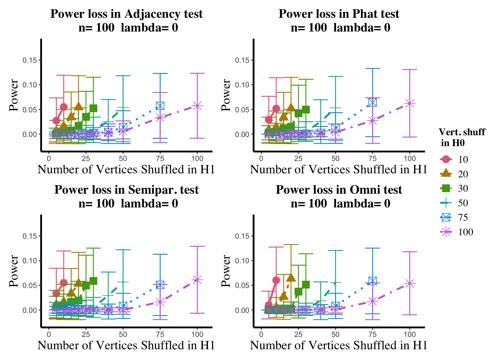
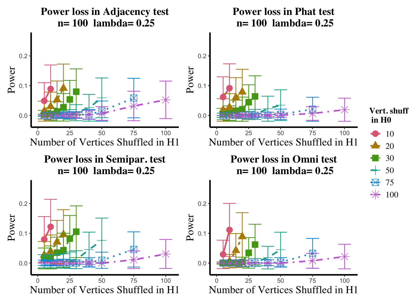
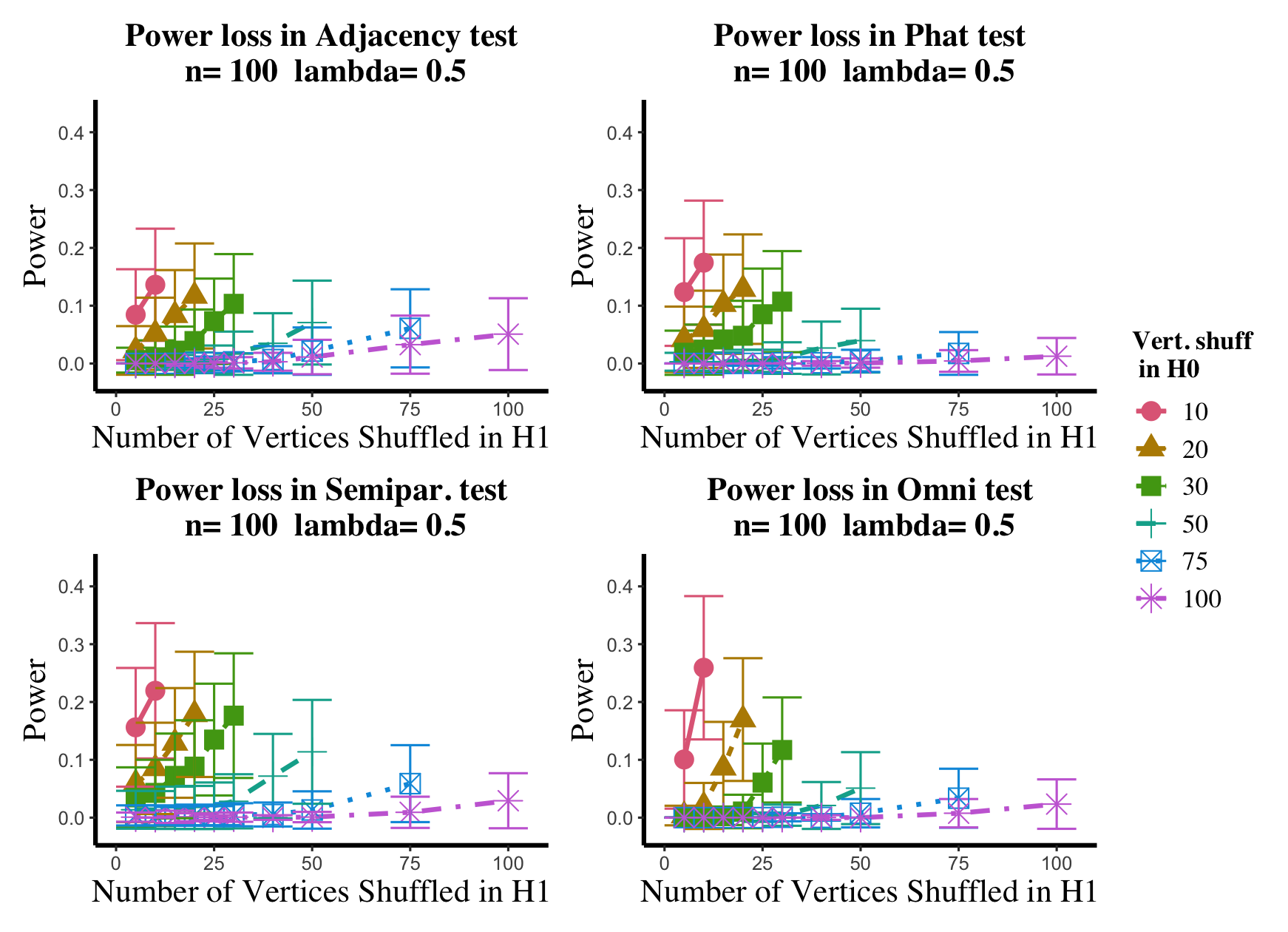
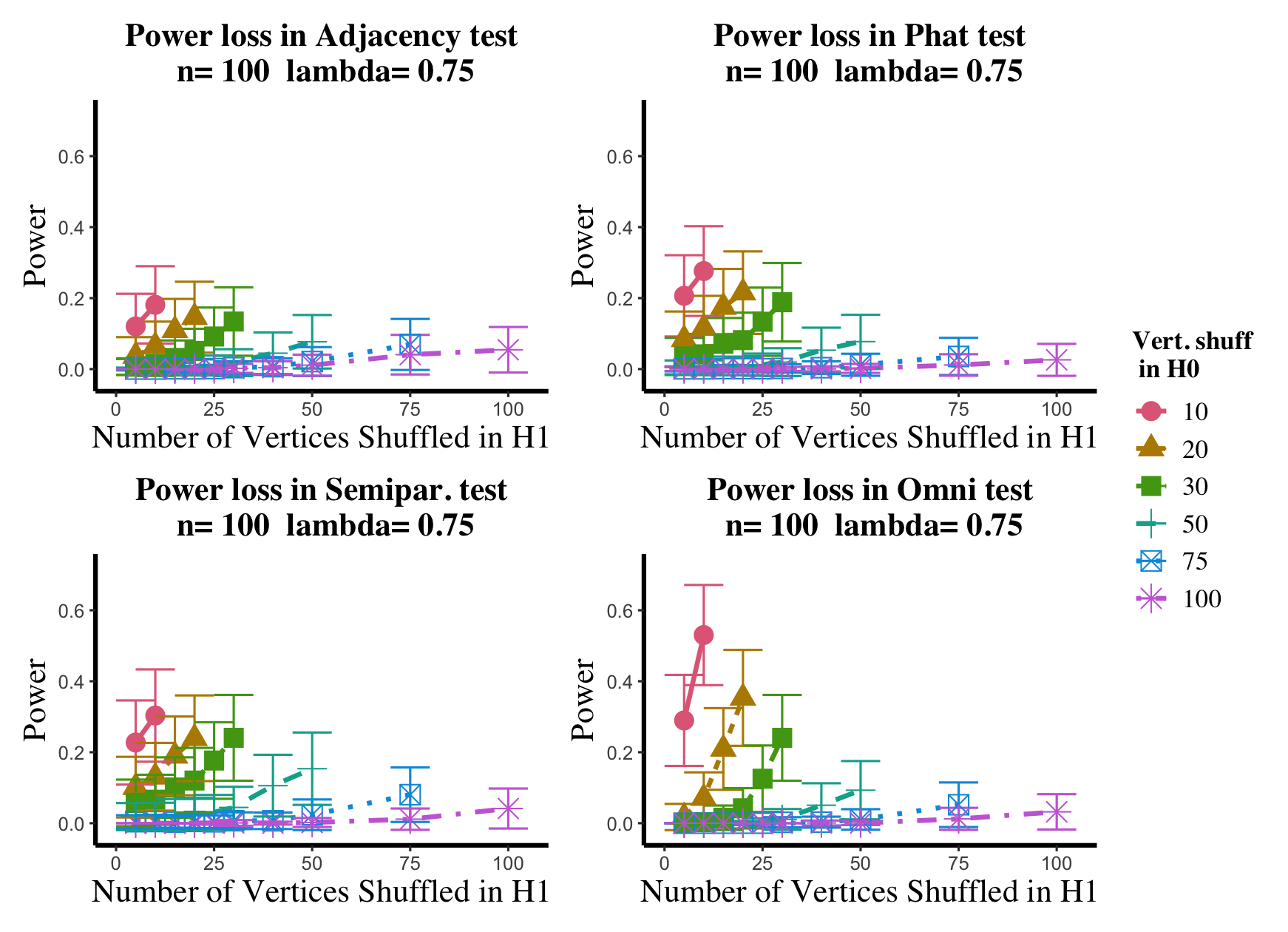
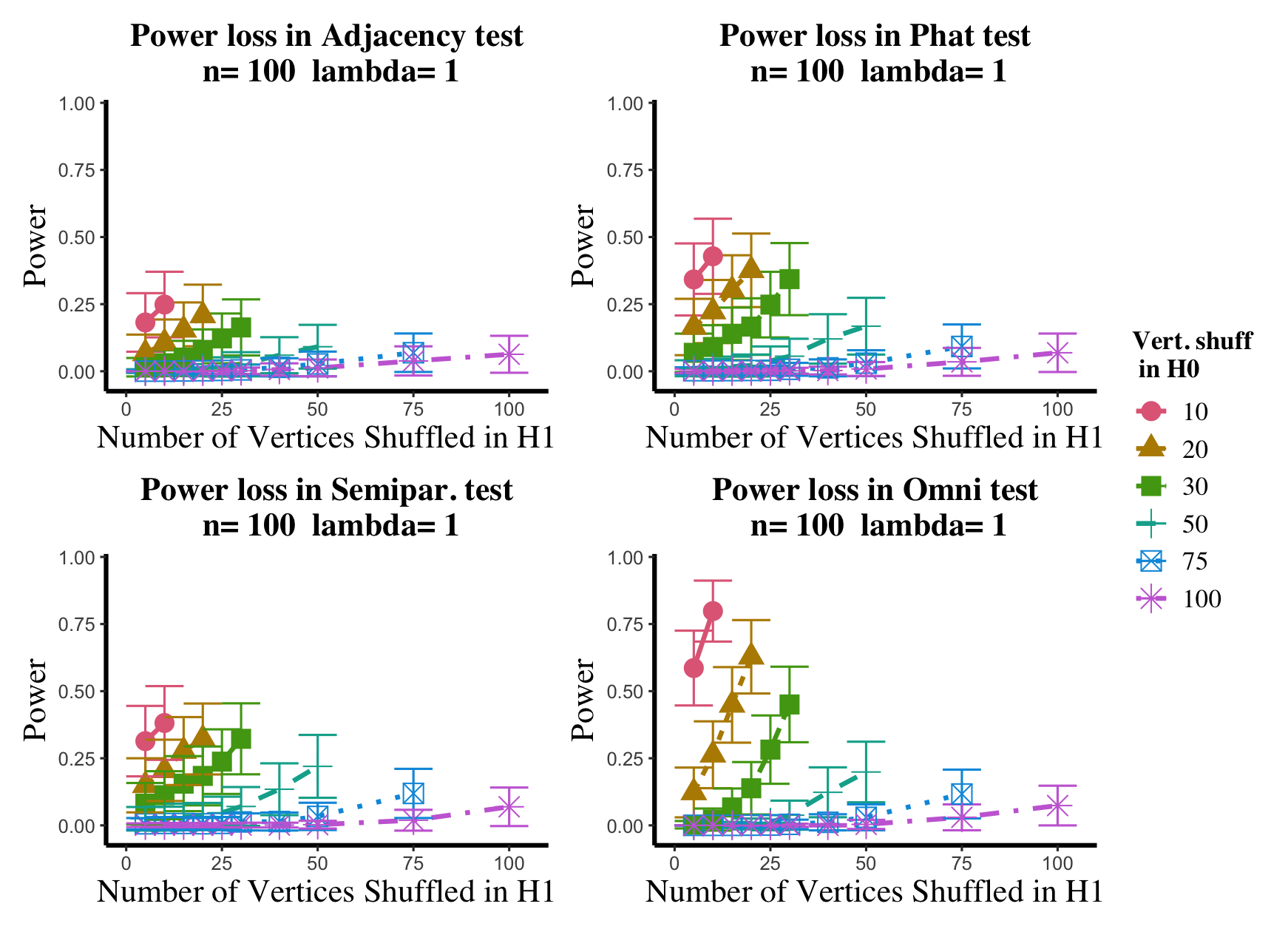
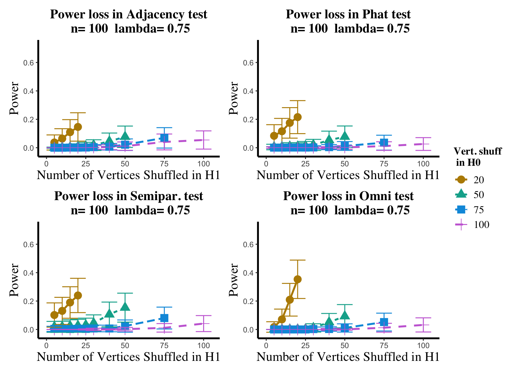
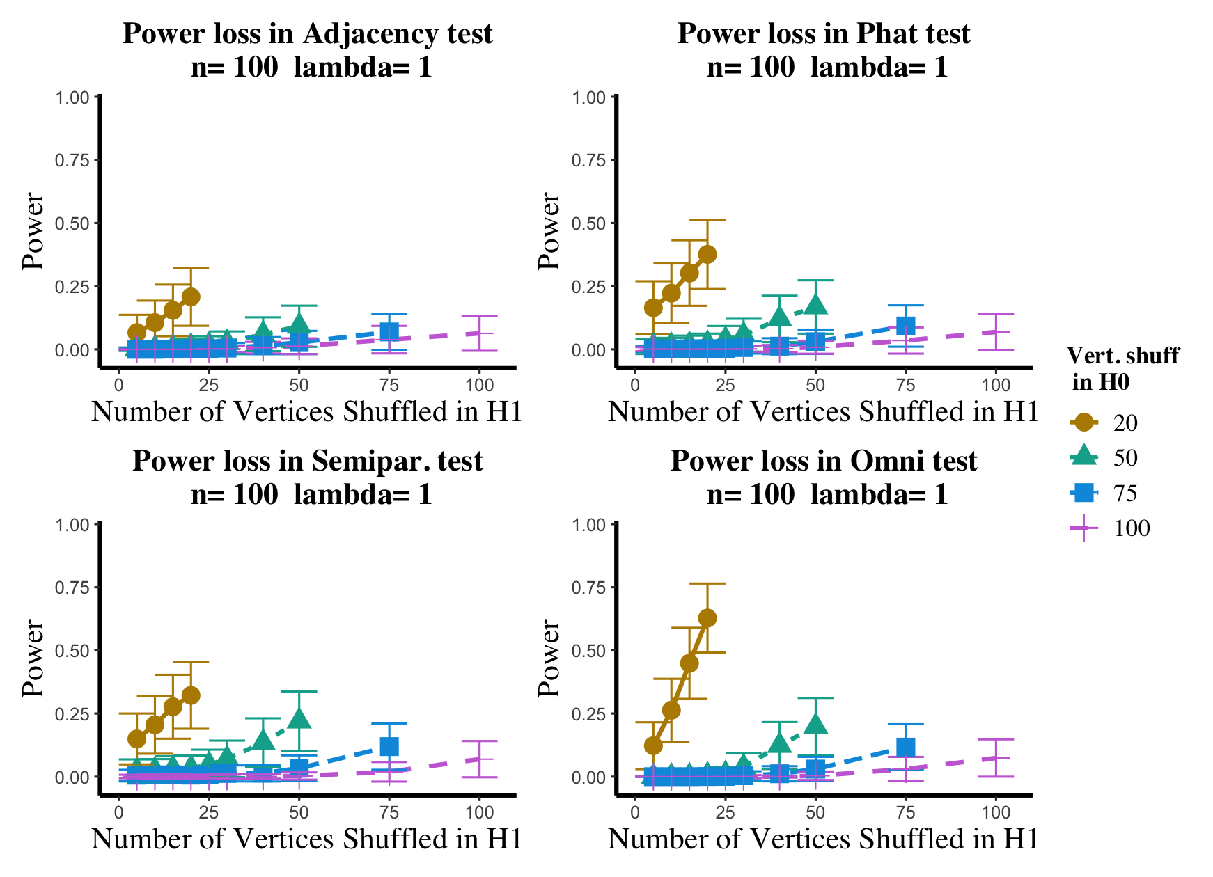
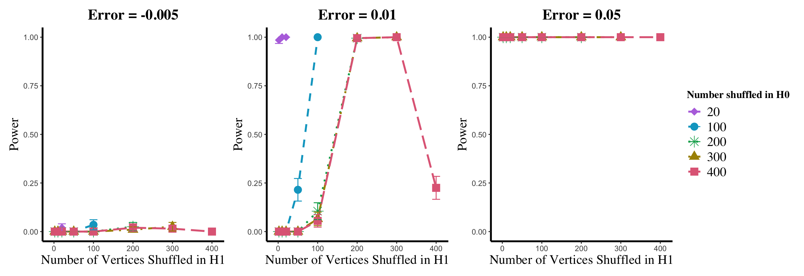
Results are displayed in Figure 5– 6 where we range (in the figures in Appendix A.4, we range ) and different values are represented by different colors/shapes of the plotted lines. Here , the number shuffled in the alternative (i.e., the number of actual incorrect labels in ), ranges over the values plotted on the -axis. Figure 5 (resp., Figure 6) show results for (resp., ); plots for the remaining values of can be found in Appendix A.4. From the figures, we see that, as expected, larger values of (i.e., more signal in the alternative) yield higher testing power, and that power diminishes greatly as the number of vertices shuffled in the null is increasing relative to the number shuffled in the alternative. We also note that the Omnibus based test appears to be more robust to shuffling than the other tests; developing analogous theory to Theorems 2.1–2.3 for the Omnibus test is a natural next step, though we do pursue this further here. We lastly note that the loss in power in the large settings is more pronounced here than in the SBM simulations, even when ; we suspect here this is due to the noise introduced by the large amount of shuffling being of higher order than the signal in the alternative.
5 Shuffling in social networks
In this section, we explore the shuffled testing phenomena in the context of the social media data found in [32]. The data contains a multilayer social network consisting of user activity across three distinct social networks: YouTube, Twitter, and FriendFeed; after initially cleaning the data (removing isolates, and symmetrizing the networks, etc.), there are a total of 422 common users across the three networks. Given adjacency matrices of our three 422-user social networks (Youtube), (Twitter), and (FriendFeed), we ultimately wish to understand the effect of vertex misalignment on testing the following hypotheses
In this case, it is difficult to get a handle on the critical values across these three tests under shuffling, so we consider the following simple initial illustrative experiment to shed light on these tests. Assuming an underlying RDPG model for each of the three networks, and using Friendfeed as our fulcrum (note that similar results are obtained using Twitter as the fulcrum network), we consider testing the simple parametric hypotheses under the effect of shuffling
| (11) |
Letting represents the edge probability matrix for the corresponding social network, we compute (similarly and ), where the embedding dimensions needed to compute ( being the ASE of the associated network) are each chosen via an automated elbow finder on the scree plot of inspired by [72] and [70], and where we then set a common embedding dimension for the three networks to the max of these three estimated dimensions.
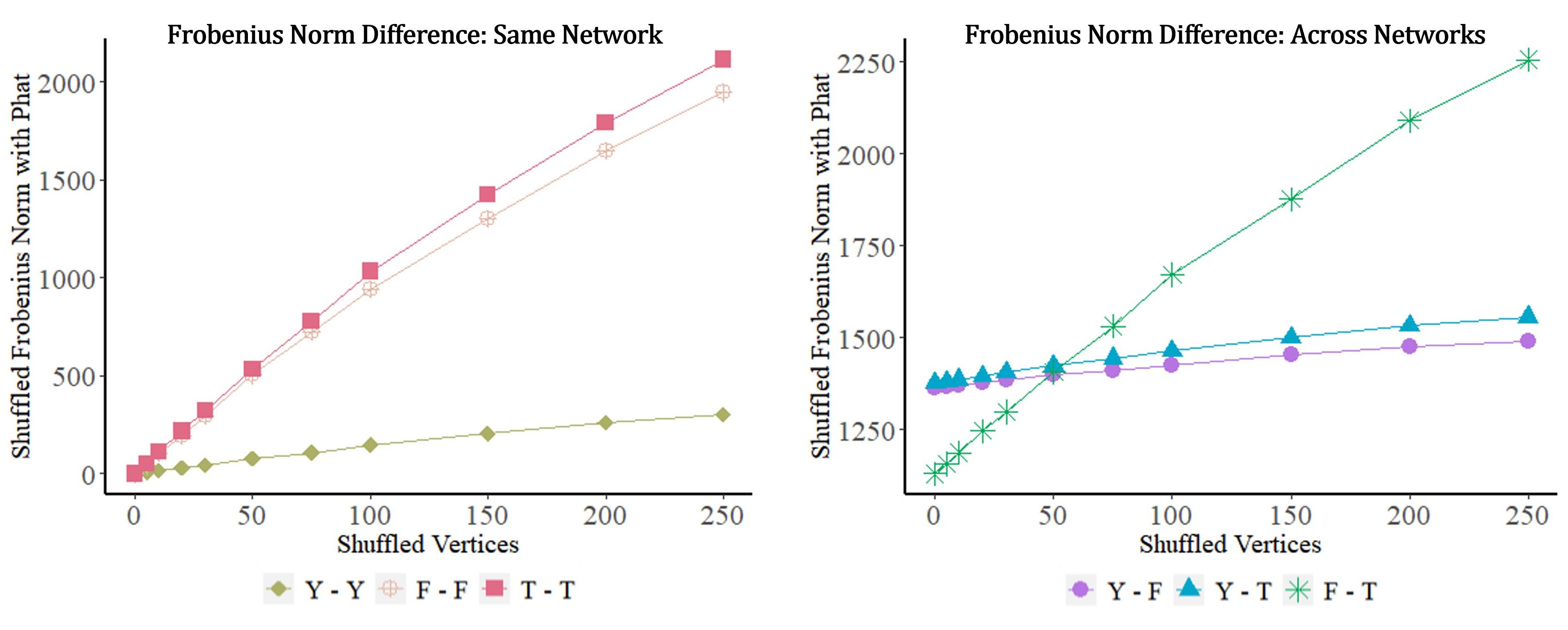
We plot these initial findings in Figure 7. In the left (resp., right) panel of the figure, we plot the Frobenius norm difference of the estimated between the same (resp., across) network as the number of shuffled vertex labels is increased within (resp., across) networks; the -axis represents the number of vertices shuffled. Note the different scales on the -axes of the two panels in the figure. From the figure, we see that although all network pairs differ significantly from each other, the FriendFeed and Twitter networks are more similar to each other (according to ) than either is to the Youtube network. However, this is obscured given enough vertex shuffling as seen by the green curve crossing the blue/purple curves in the right panel. Given enough uncertainty in the vertex labels, we posit that a conservative test using —i.e., one that must assume the uncertain labels are shuffled—would compute the FriendFeed and Twitter networks to be more similar to each other (if the uncertain labels are, in fact, correct and not shuffled under ) than either is to themselves, and so we should be less likely to reject of Eq. 11.
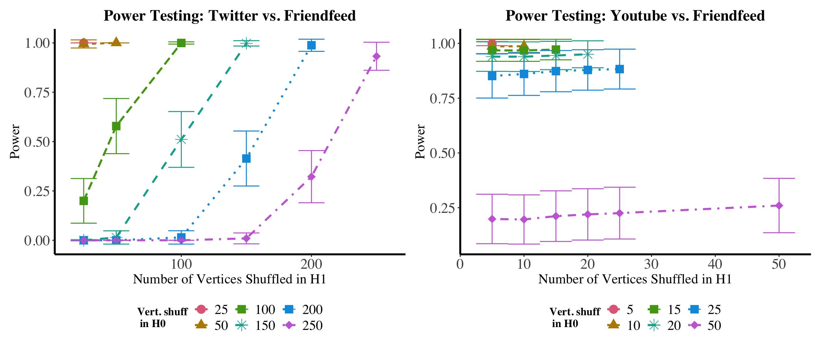
We see this play out in Figure 8, where we use a parametric bootstrap (assuming the RDPG model framework) with 200 bootstrapped replicates to estimate each of the critical values and the testing power in order to see the effect of vertex shuffling on the testing power for and of Eq. 11; note that as in section 1.3 we consider the following modification of the overall testing regime: We consider a fixed (randomly chosen) sequence of nested permutations for for and for . We consider shuffling the null by and the alternative by for all . We then repeat this process times, each time obtaining a bootstrapped estimate of testing power against . In the figure, we plot the average empirical testing power, where the amount shuffled in the conservative null is (so that is entirely shuffled); the different colored curves represent the different -values. The amount actually shuffled in the alternative, , is plotted on the -axis. From the figure, we see that the test would reject the null in both cases when few vertices are shuffled (i.e., a small -value) or when is small in the Twitter versus Friendfeed panel; this is as expected from Figure 7, as the networks all seem to differ significantly from each other. However, testing power degrades significantly when is large in the Twitter versus Friendfeed setting and in the large setting for Youtube versus Friendfeed, and the test no longer rejects the null. While the former is as expected—indeed, with enough uncertainty the small differences across the Twitter and Youtube networks is lost in the shuffle, even when the networks are different—the latter is surprising. Further investigation yields that this power degradation as a function of alone stems from a difference in density, as the Youtube network is sparse and ; in this case the error in shuffling under the null when is large overwhelms any effect of shuffling in the alternative.
If the sparse Youtube network is used as the fulcrum, then both power figures would have power equal to one uniformly. The sparse Youtube graph is markedly different in degree from the two denser networks, and the shuffling does not affect that difference. In general, testing for a measure of equality in graphs with markedly different degree distributions would require a modified version of the hypotheses and test statistic, perhaps of the form (inspired by [11]) for a scaling constant (to test equality of latent positions up to rotation and constant scaling) or for a diagonal scaling matrix (to test equality of latent positions up to rotation and diagonal scaling).
6 Graph matching (unshuffling)
Once we quantify the added uncertainty due to shuffles in the vertex correspondences, it is natural to try to remedy this shuffling via graph matching. In this context, the graph matching problem seeks the correspondence between the vertices of the graphs that minimizes the number of induced edge disagreements [37]. Formally, letting again denote the sets of permutations matrices, the simplest formulation of the graph matching problem can be cast as seeking elements in . For a survey on the current state of the graph matching literature, see [35, 36, 37].
The problem of graph matching can often be made easier by having prior information about the true vertex correspondence. This information can come in the form of seeds, or a list of vertices for which the true, latent correspondence is known a priori; see [75, 47, 76]. In the current shuffled testing regime, only the vertices of have unknown correspondence, and so the graph matching problem would reduce to seeking elements in ; i.e., those vertices in can be treated as seeds. While there are no efficient algorithms known for matching in general (with or without seeds), there are a number of approximate seeded graph matching algorithms (see, for example, [47, 76]) that have proven effective in practice. In applications below, we will make use of the SGM algorithm of [47] to approximately solve the seeded graph matching problem.
6.1 SBM Shuffling and Matching
We first begin by testing the dual effects of shuffling and matching on testing power in the SBM setting (where, as in Section 3.0.1, the critical values and the power can be computed via direct simulation). Adopting the notation of Section 2.1.2, we first consider an SBM with vertices, where is given by:
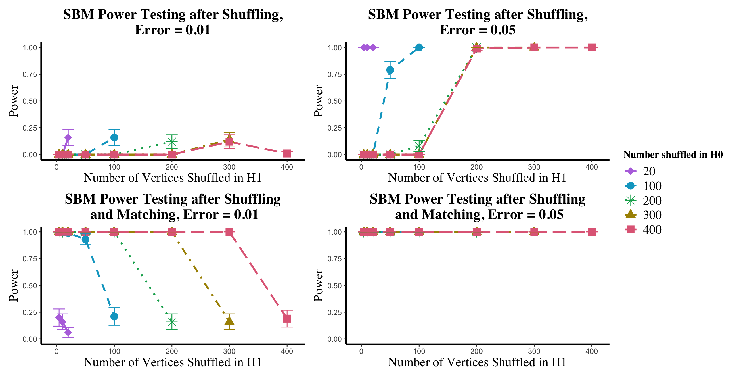
Letting (, so that vertices are shuffled between each of the two blocks) be as defined in Section 2.1.2, we consider the error matrix ; in this example we will consider . In this setting, we will simulate directly (using the true model parameters) from the SBM models to estimate the relevant critical values and the testing powers; here, all critical values and power estimates are based on Monte Carlo replicates.
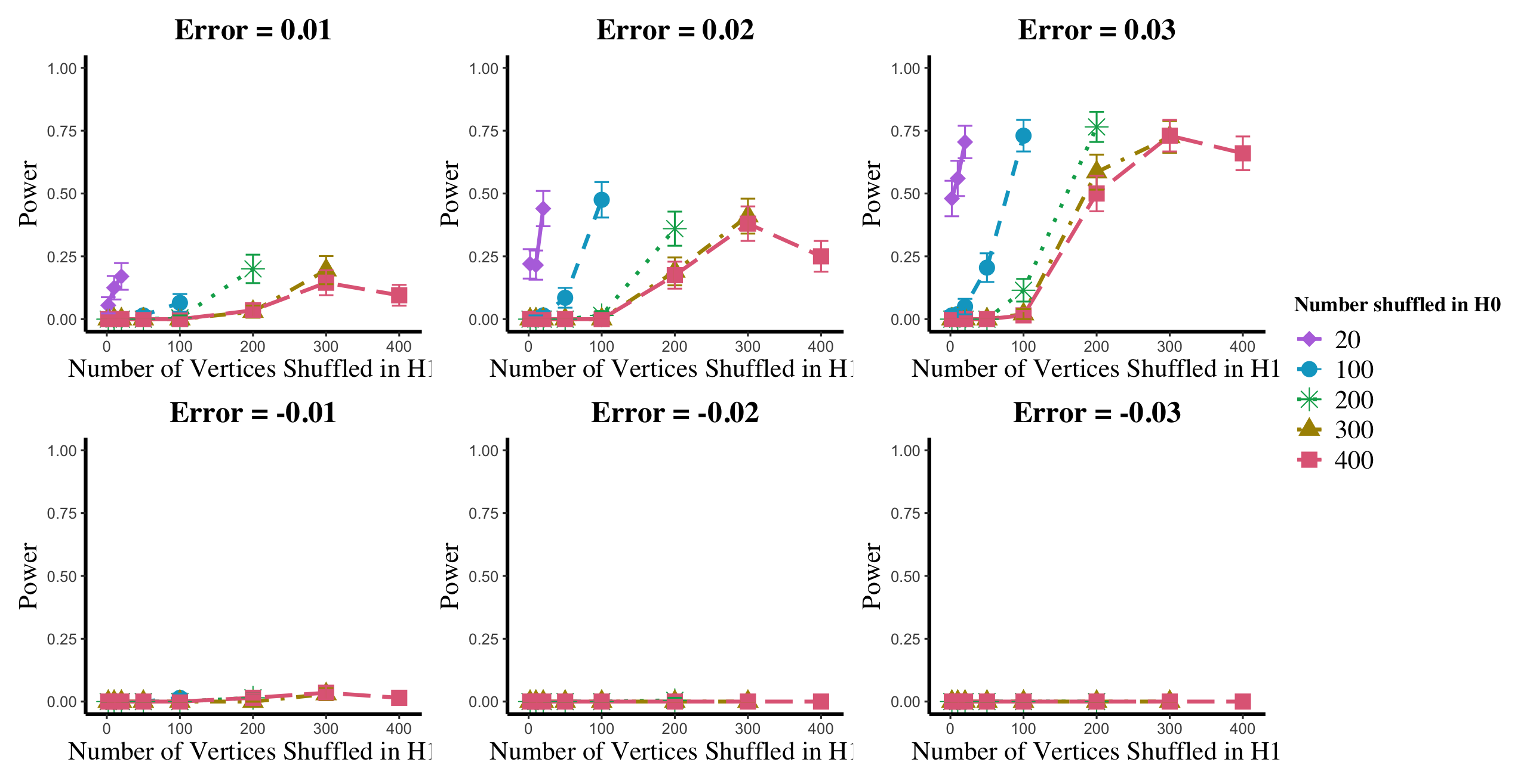
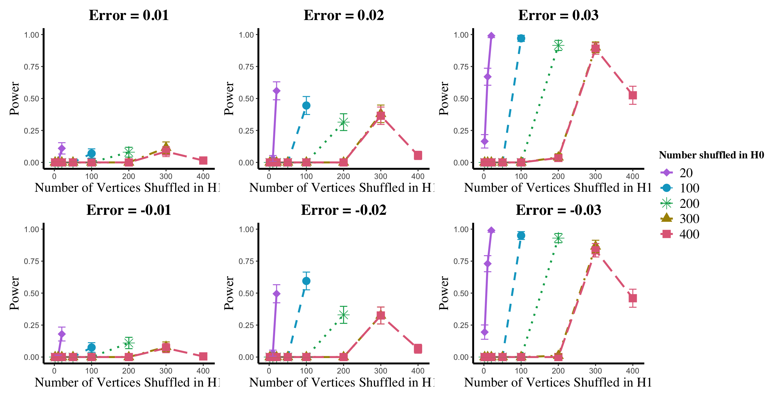
In Figures 9, we plot (in the upper panels) the power loss due to shuffling in the and settings; in the bottom panels, we plot the effect of shuffling and then matching on testing power (where we first match the graphs, and then use the unshuffled statistic for the hypothesis test. For each , we would (in practice) use SGM to unshuffle all vertices in regardless of the value of —represented here by the unshuffling in the case. Here, we also show the effect of unshuffling only the vertices truly shuffled in the alternative. From the case, we see that matching recovers the lost shuffling power. From the setting, we see that the (possible) downside of unshuffling is its propensity to align the two graphs better than the true, latent alignment. In general, the more vertices being matched, the smaller the graph matching objective function, and hence the smaller the test statistic, which here manifests as larger than desired type-I error probability. Note that in each ASE used to compute in this experiment, we used the true value of .
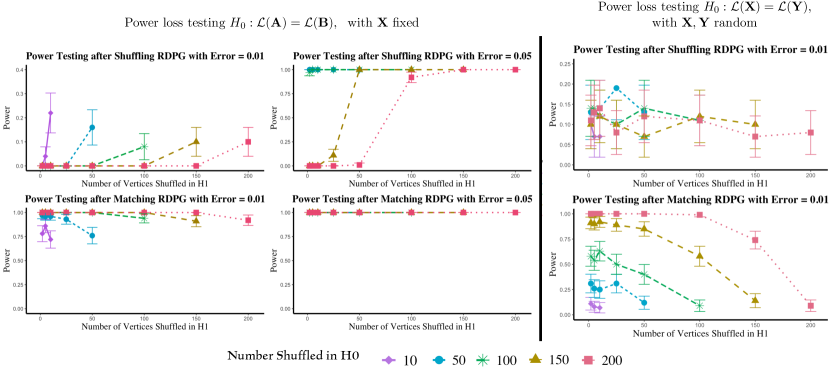
These results play out in more general random graph settings as well, with Figure 10, showing the corresponding results in the RDPG setting of Section 4; i.e., each graph is vertices with the rows of X are i.i.d. Dirichlet(1,1,1). The error here is added directly to the latent positions, as for , and . In the left panels, where we are fixing the latent positions and testing , the results are similar: unshuffling recovering the testing power, and over-matching providing artificially high testing power. In the right panel, we show results for testing where the latent positions are random and the rows of X are i.i.d. In this case, shuffling has no effect on testing power (as seen in the upper panel), while over-matching can still detrimentally add artificial power (as seen in the lower panel).
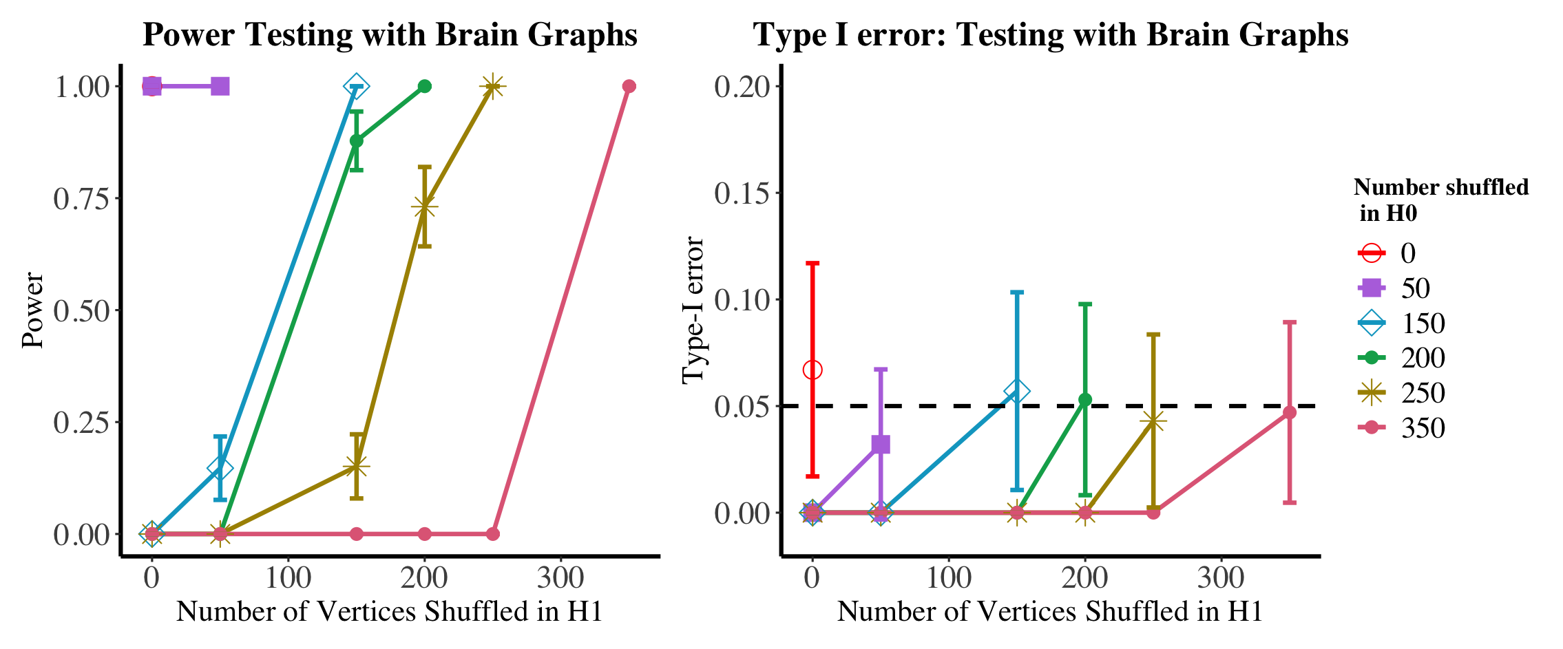
6.2 Brain networks shuffling and matching
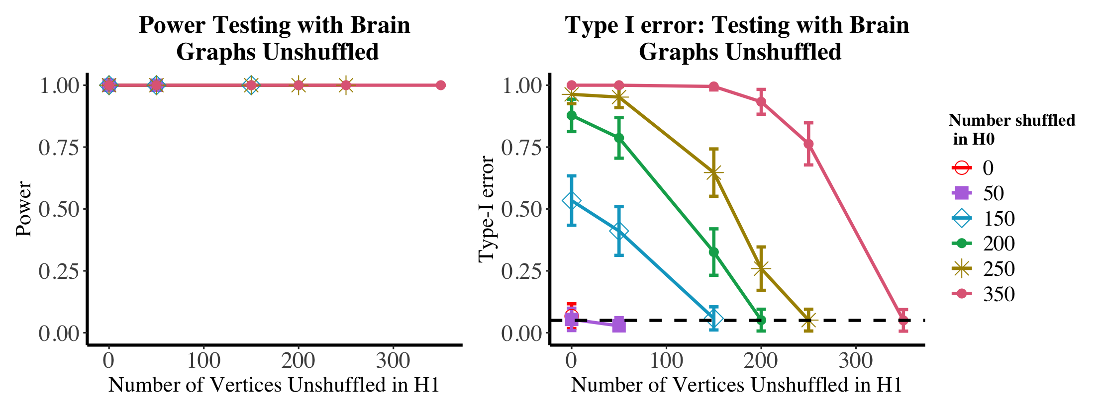
We explore the dual effects of shuffling and matching on testing power in the motivating brain testing example of Section 1.3 (again with 200 bootstrap samples and averaged over nMC=100 Monte Carlo trials). In Figures 11, we plot (in the left panel) the power of the test when the brains are shuffled, then matched before testing (the power here is estimated using the parametric bootstrap procedure outlined in Section 1.3); note, as we first match the graphs we use the unshuffled statistic for this hypothesis test, i.e., we use when estimating the null critical value, and when estimating the testing power. Again, we show the effect of unshuffling all unknown vertices in the null and only the vertices truly shuffled in the alternative. As in the simulations, from the case, we see that matching recovers the lost shuffling power while maintaining the desired testing level. From the setting, we see that this recovered power is at the expense of testing level much greater than the desired . In the event that the matching is viewed as a pre-processing step, matching more vertices in the null than the alternative could increase the true level of the test resulting in heightened type-I error risk (resulting in possibly artificially high testing power) as seen in the right panel of Figure 11.
7 Conclusions
As network data has become more commonplace, a number of statistical tools tailored for handling network data have been developed, including methods for hypothesis testing, goodness-of-fit analysis, clustering, and classification among others. Classically, many of the paired or multiple network inference tasks have assumed the vertices are aligned across networks, and this known alignment is often leveraged to improve subsequent inference. Exploring the impact of shuffled/misaligned vertices on inferential performance—here on testing power—is an increasingly important problem as these methods gain more traction in noisy network domains. By systematically breaking down a simple Frobenius-norm hypothesis test, we uncover and numerically analyze the decline of power as a function of both the distributional difference in the alternative and the number of shuffled nodes. Further analysis in a pair of real data settings reinforce our findings in giving practical guidance for the level of tolerable noise in paired, vertex-aligned testing procedures.
Our most thorough analysis of power loss is done in the context of random dot product and stochastic block models; bolstered by extensive simulation with real data experiments backing up our findings. While the goal of our research is to test the robustness of multiple network hypothesis testing methodologies, there still remains work to do in extending our findings to more general network models and to more complex network testing paradigms. A natural next step is to lift the simple Frobenius norm hypothesis test analysis to more broad and complex models, as well as test misalignment of vertices in the Omnibus and Semiparametric testing settings (see Section 4). Within the context of SBM’s we aim to see how our power analysis changes for more esoteric shufflings (more blocks, different number flipped between blocks, etc.). Further extensions include extending the theory to non-edge independent graph models, and to shuffling in two sample tests where there are multiple graphs per sample, and where there is an interplay to explore in shuffling within and across populations. In non-testing inference tasks, often the vertices are assumed aligned as well (e.g., tensor factorization, multiple graph embeddings, etc.), and exploring the inferential performance loss due to shuffled vertices in these settings is a natural next step.
In the event that vertex labels are incorrectly known, it is natural to use a graph matching/network alignment methods to align the networks before proceeding with subsequent inference. There are a host of matching procedures in the literature that could be applied to recover the true vertex alignment, and in doing so recover the lost testing power [40]. We explore this in the context of our simulations and find that while matching recovers the lost power, “over matching” can result in artificially high power. Care must be taken when using alignment tools for data pre-processing, as graph matching methods can induce artificial signal across even disparate network pairs (this is related to the “phantom alignment strength” phenomena of [77]). Natural next steps in this direction include the following questions (among others): how the signal in an imperfectly recovered matching affects power loss as opposed to a random misalignment; how a probabilistic alignment (where the unknown in vertex labels is encoded into a stochastic matrix giving probabilities of alignment) can be incorporated into the testing framework; and how to use matching metrics (e.g., alignment strength [50, 77]) to estimate the size and membership of when this is unknown a priori.
Acknowledgements: This material is based on research sponsored by the Air Force Research Laboratory (AFRL) and Defense Advanced Research Projects Agency (DARPA) under agreement number FA8750-20-2-1001. The U.S. Government is authorized to reproduce and distribute reprints for Governmental purposes notwithstanding any copyright notation thereon. The views and conclusions contained herein are those of the authors and should not be interpreted as necessarily representing the official policies or endorsements, either expressed or implied, of the AFRL and DARPA or the U.S. Government.
References
- [1] A. Goldenberg, A. X. Zheng, S. E. Fienberg, E. M. Airoldi, A survey of statistical network models, Found. Trends Mach. Learn. 2 (2) (2009) 129–233. arXiv:0912.5410, doi:10.1561/2200000005.
- [2] E. Bullmore, O. Sporns, Complex brain networks: graph theoretical analysis of structural and functional systems, Nature reviews neuroscience 10 (3) (2009) 186–198.
- [3] D. Durante, D. B. Dunson, Bayesian inference and testing of group differences in brain networks, Bayesian Analysis 13 (1) (2018) 29–58.
- [4] J. Chung, E. Bridgeford, J. Arroyo, B. D. Pedigo, A. Saad-Eldin, V. Gopalakrishnan, L. Xiang, C. E. Priebe, J. T. Vogelstein, Statistical connectomics, Annu. Rev. Stat. Appl. 8 (2021) 463–492.
- [5] J. C. Mitchell, Social networks, Annual review of anthropology 3 (1) (1974) 279–299.
- [6] P. J. Carrington, J. Scott, S. Wasserman, Models and methods in social network analysis, Vol. 28, Cambridge university press, 2005.
- [7] A. Vazquez, A. Flammini, A. Maritan, A. Vespignani, Global protein function prediction from protein-protein interaction networks, Nature biotechnology 21 (6) (2003) 697–700.
- [8] O. N. Temkin, A. V. Zeigarnik, D. Bonchev, Chemical reaction networks: a graph-theoretical approach, CRC Press, 2020.
- [9] E. D. Kolaczyk, Statistical Analysis of Network Data: Methods and Models, Springer Science & Business Media, 2009.
- [10] E. D. Kolaczyk, G. Csárdi, Statistical analysis of network data with R, Vol. 65, Springer, 2014.
- [11] M. Tang, A. Athreya, D. L. Sussman, V. Lyzinski, Y. Park, C. E. Priebe, A semiparametric two-sample hypothesis testing problem for random graphs, Journ. of Computational and Graphical Statistics 26 (2) (2017) 344–354.
- [12] M. Tang, A. Athreya, D. L. Sussman, V. Lyzinski, C. E. Priebe, A nonparametric two-sample hypothesis testing problem for random graphs, Bernoulli 23 (3) (2017) 1599–1630. arXiv:arXiv:1409.2344, doi:10.3150/15-BEJ789.
- [13] C. E. Ginestet, J. Li, P. Balachandran, S. Rosenberg, E. D. Kolaczyk, Hypothesis testing for network data in functional neuroimaging, Ann. Appl. Stat. (2017) 725–750.
- [14] D. R. Hunter, S. M. Goodreau, M. S. Handcock, Goodness of fit of social network models, J. Am. Stat. Assoc. 103 (481) (2008) 248–258.
- [15] J. Lei, A goodness-of-fit test for stochastic block models, Ann. Stat. 44 (1) (2016) 401–424.
- [16] Y. R. Wang, P. J. Bickel, Likelihood-based model selection for stochastic block models, Ann. Stat. 45 (2) (2017) 500–528.
- [17] M. E. Newman, Clustering and preferential attachment in growing networks, Physical review E 64 (2) (2001) 025102.
- [18] A. Clauset, M. E. Newman, C. Moore, Finding community structure in very large networks, Physical review E 70 (6) (2004) 066111.
- [19] V. D. Blondel, J.-L. Guillaume, R. Lambiotte, E. Lefebvre, Fast unfolding of communities in large networks, Journ. of statistical mechanics: theory and experiment 2008 (10) (2008) P10008.
- [20] K. Rohe, S. Chatterjee, B. Yu, Spectral clustering and the high-dimensional stochastic blockmodel, Ann. Stat. 39 (4) (2011) 1878–1915.
- [21] D. L. Sussman, M. Tang, D. E. Fishkind, C. E. Priebe, A consistent adjacency spectral embedding for stochastic blockmodel graphs, J. Am. Stat. Assoc. 107 (499) (2012) 1119–1128. arXiv:1108.2228, doi:10.1080/01621459.2012.699795.
- [22] J. Lei, A. Rinaldo, Consistency of spectral clustering in stochastic block models, Ann. Stat. 43 (1) (2015) 215–237.
- [23] J. T. Vogelstein, C. E. Priebe, Shuffled graph classification: Theory and connectome applications, J. Classif. 32 (1) (2015) 3–20.
- [24] M. Tang, D. L. Sussman, C. E. Priebe, Universally consistent vertex classification for latent positions graphs, Ann. Stat. 41 (3) (2013) 1406–1430.
- [25] V. Lyzinski, M. Tang, A. Athreya, Y. Park, C. E. Priebe, Community detection and classification in hierarchical stochastic blockmodels, IEEE Trans. on Network Science and Engineering 4 (1) (2016) 13–26.
- [26] M. Zhang, Z. Cui, M. Neumann, Y. Chen, An end-to-end deep learning architecture for graph classification, in: Thirty-Second AAAI Conf. on Artificial Intelligence, 2018.
- [27] D. Durante, D. B. Dunson, J. T. Vogelstein, Nonparametric bayes modeling of populations of networks, Journal of the American Statistical Association 112 (520) (2017) 1516–1530.
-
[28]
J. Arroyo, A. Athreya, J. Cape, G. Chen, C. E. Priebe, J. T. Vogelstein,
Inference for multiple heterogeneous
networks with a common invariant subspace (2019) 1–45arXiv:1906.10026.
URL http://arxiv.org/abs/1906.10026 - [29] V. Lyzinski, D. L. Sussman, Matchability of heterogeneous networks pairs, Information and Inference: A Journal of the IMA 9 (4) (2020) 749–783.
- [30] B. Viswanath, A. Mislove, M. Cha, K. P. Gummadi, On the evolution of user interaction in facebook, in: Proceedings of the 2nd ACM workshop on Online social networks, 2009, pp. 37–42.
- [31] M. Heimann, H. Shen, T. Safavi, D. Koutra, Regal: Representation learning-based graph alignment, in: Proceedings of the 27th ACM international conference on information and knowledge management, 2018, pp. 117–126.
- [32] M. Magnani, L. Rossi, The ml-model for multi-layer social networks, in: Inter. Conf. Adv. Soc Netw Anal Min, IEEE, 2011, pp. 5–12.
- [33] H. G. Patsolic, Y. Park, V. Lyzinski, C. E. Priebe, Vertex nomination via seeded graph matching, Statistical Analysis and Data Mining: The ASA Data Science Journal 13 (3) (2020) 229–244.
- [34] R. Mastrandrea, J. Fournet, A. Barrat, Contact patterns in a high school: a comparison between data collected using wearable sensors, contact diaries and friendship surveys, PloS one 10 (9) (2015) e0136497.
- [35] D. Conte, P. Foggia, C. Sansone, M. Vento, Thirty years of graph matching in pattern recognition, Intern J Pattern Recognit Artif Intell 18 (03) (2004) 265–298.
- [36] P. Foggia, G. Percannella, M. Vento, Graph matching and learning in pattern recognition in the last 10 years, Intern J Pattern Recognit Artif Intell 28 (01) (2014) 1450001.
- [37] J. Yan, X.-C. Yin, W. Lin, C. Deng, H. Zha, X. Yang, A short survey of recent advances in graph matching, in: Proceedings of the 2016 ACM on International Conf. on Multimedia Retrieval, 2016, pp. 167–174.
- [38] B. D. Pedigo, M. Winding, C. E. Priebe, J. T. Vogelstein, Bisected graph matching improves automated pairing of bilaterally homologous neurons from connectomes, Network Neuroscience 7 (2) (2023) 522–538.
- [39] M. Fiori, P. Sprechmann, J. Vogelstein, P. Musé, G. Sapiro, Robust multimodal graph matching: Sparse coding meets graph matching, Advances in neural information processing systems 26 (2013).
- [40] V. Lyzinski, Information recovery in shuffled graphs via graph matching, IEEE Trans. on Information Theory 64 (5) (2018) 3254–3273.
- [41] G. Chen, J. Arroyo, A. Athreya, J. Cape, J. T. Vogelstein, Y. Park, C. White, J. Larson, W. Yang, C. E. Priebe, Multiple network embedding for anomaly detection in time series of graphs, arXiv preprint arXiv:2008.10055 (2020).
- [42] L. Chen, J. Zhou, L. Lin, Hypothesis testing for populations of networks, Communications in Statistics-Theory and Methods 52 (11) (2023) 3661–3684.
- [43] X. Du, M. Tang, Hypothesis testing for equality of latent positions in random graphs, Bernoulli 29 (4) (2023) 3221–3254.
- [44] D. Asta, C. R. Shalizi, Geometric network comparison, Proceedings of the 31st Annual Conference on Uncertainty in AI (UAI) (2015).
- [45] K. Levin, A. Athreya, M. Tang, V. Lyzinski, C. E. Priebe, A central limit theorem for an omnibus embedding of multiple random dot product graphs, 2017 IEEE inter. conf. on data mining workshops (2017) 964–967.
- [46] J. Agterberg, M. Tang, C. Priebe, Nonparametric two-sample hypothesis testing for random graphs with negative and repeated eigenvalues, arXiv preprint arXiv:2012.09828 (2020).
- [47] D. E. Fishkind, S. Adali, H. G. Patsolic, L. Meng, D. Singh, V. Lyzinski, C. E. Priebe, Seeded graph matching, Pattern Recognit. 87 (2019) 203–215.
- [48] G. Coppersmith, Vertex nomination, Wiley Interdisciplinary Reviews: Computational Statistics 6 (2) (2014) 144–153.
- [49] D. E. Fishkind, V. Lyzinski, H. Pao, L. Chen, C. E. Priebe, Vertex nomination schemes for membership prediction, Ann. Appl. Stat. 9 (3) (2015) 1510–1532.
- [50] D. E. Fishkind, L. Meng, A. Sun, C. E. Priebe, V. Lyzinski, Alignment strength and correlation for graphs, Pattern Recognit. Lett. 125 (2019) 295–302.
- [51] K. Levin, E. Levina, Bootstrapping networks with latent space structure, arXiv preprint arXiv:1907.10821 (2019).
- [52] X. Zuo, J. S. Anderson, P. Bellec, R. M. Birn, B. B. Biswal, J. Blautzik, J. C. Breitner, R. L. Buckner, V. D. Calhoun, F. X. Castellanos, et al., An open science resource for establishing reliability and reproducibility in functional connectomics, Scientific data 1 (1) (2014) 1–13.
- [53] G. Kiar, E. W. Bridgeford, W. R. G. Roncal, C. for Reliability, R. (CoRR), V. Chandrashekhar, D. Mhembere, S. Ryman, X. Zuo, D. S. Margulies, R. C. Craddock, et al., A high-throughput pipeline identifies robust connectomes but troublesome variability, bioRxiv (2017) 188706.
- [54] S. J. Young, E. R. Scheinerman, Random dot product graph models for social networks, in: International Workshop on Algorithms and Models for the Web-Graph, Springer, 2007, pp. 138–149.
- [55] A. Athreya, D. E. Fishkind, M. Tang, C. E. Priebe, Y. Park, J. T. Vogelstein, K. Levin, V. Lyzinski, Y. Qin, D. L. Sussman, Statistical inference on random dot product graphs: A survey, J. Mach. Learn. Res. 18 (2018) 1–92.
- [56] P. D. Hoff, A. E. Raftery, M. S. Handcock, Latent space approaches to social network analysis, J. Am. Stat. Assoc. 97 (460) (2002) 1090–1098.
- [57] P. W. Holland, K. B. Laskey, S. Leinhardt, Stochastic blockmodels: First steps, Social networks 5 (2) (1983) 109–137.
- [58] E. M. Airoldi, D. M. Blei, S. E. Fienberg, E. P. Xing, Mixed membership stochastic blockmodels, J. Mach. Learn. Res. (2008).
- [59] B. Karrer, M. E. J. Newman, Stochastic blockmodels and community structure in networks, Physical review E 83 (1) (2011) 016107.
- [60] T. Li, L. Lei, S. Bhattacharyya, K. Van den Berge, P. Sarkar, P. J. Bickel, E. Levina, Hierarchical community detection by recursive partitioning, J. Am. Stat. Assoc. (2020) 1–18.
- [61] P. Rubin-Delanchy, J. Cape, M. Tang, C. E. Priebe, A statistical interpretation of spectral embedding: the generalised random dot product graph, J. R. Stat. Soc. Series B to appear (2022).
- [62] D. L. Sussman, M. Tang, C. E. Priebe, Consistent latent position estimation and vertex classification for random dot product graphs, IEEE Trans. Pattern Anal. Mach. Intell. 36 (1) (2014) 48–57. arXiv:arXiv:1207.6745v1, doi:10.1109/TPAMI.2013.135.
- [63] I. Gallagher, A. Jones, A. Bertiger, C. E. Priebe, P. Rubin-Delanchy, Spectral embedding of weighted graphs, Journal of the American Statistical Association (2023) 1–10.
- [64] V. Lyzinski, D. L. Sussman, M. Tang, A. Athreya, C. E. Priebe, Perfect clustering for stochastic blockmodel graphs via adjacency spectral embedding, Electron. J. Stat. 8 (2014) 2905–2922. arXiv:1310.0532, doi:10.1214/14-EJS978.
- [65] A. Athreya, C. E. Priebe, M. Tang, V. Lyzinski, D. J. Marchette, D. L. Sussman, A limit theorem for scaled eigenvectors of random dot product graphs, Sankhya A 78 (2016) 1–18.
- [66] F. Sanna Passino, N. A. Heard, P. Rubin-Delanchy, Spectral clustering on spherical coordinates under the degree-corrected stochastic blockmodel, Technometrics (just-accepted) (2021) 1–28.
- [67] K. Pantazis, A. Athreya, W. N. Frost, E. S. Hill, V. Lyzinski, The importance of being correlated: Implications of dependence in joint spectral inference across multiple networks, Journal of Machine Learning Research 23 (141) (2022) 1–77.
- [68] J. Yoder, L. Chen, H. Pao, E. Bridgeford, K. Levin, D. E. Fishkind, C. Priebe, V. Lyzinski, Vertex nomination: The canonical sampling and the extended spectral nomination schemes, Computational Statistics & Data Analysis 145 (2020) 106916.
- [69] D. E. Fishkind, D. L. Sussman, M. Tang, J. T. Vogelstein, C. E. Priebe, Consistent adjacency-spectral partitioning for the stochastic block model when the model parameters are unknown, SIAM Journ. on Matrix Analysis and Applications 34 (1) (2013) 23–39.
- [70] S. Chatterjee, Matrix estimation by universal singular value thresholding, Ann. Stat. 43 (1) (2015) 177–214.
- [71] T. Li, E. Levina, J. Zhu, Network cross-validation by edge sampling, Biometrika 107 (2) (2020) 257–276.
- [72] M. Zhu, A. Ghodsi, Automatic dimensionality selection from the scree plot via the use of profile likelihood, Computational Statistics & Data Analysis 51 (2) (2006) 918–930.
- [73] B. Draves, D. L. Sussman, Bias-variance tradeoffs in joint spectral embeddings, arXiv preprint arXiv:2005.02511 (2020).
- [74] K. Levin, A. Athreya, M. Tang, V. Lyzinski, Y. Park, C. E. Priebe, A central limit theorem for an omnibus embedding of multiple random graphs and implications for multiscale network inference, arXiv preprint arXiv:1705.09355 (2017).
- [75] F. Fang, D. L. Sussman, V. Lyzinski, Tractable graph matching via soft seeding, arXiv preprint arXiv:1807.09299 (2018).
- [76] E. Mossel, J. Xu, Seeded graph matching via large neighborhood statistics, Random Structures & Algorithms 57 (3) (2020) 570–611.
- [77] D. E. Fishkind, F. Parker, H. Sawczuk, L. Meng, E. Bridgeford, A. Athreya, C. Priebe, V. Lyzinski, The phantom alignment strength conjecture: practical use of graph matching alignment strength to indicate a meaningful graph match, Appl. Netw. Sci. 6 (1) (2021) 1–27.
- [78] C. Stein, Approximate computation of expectations, IMS, 1986.
- [79] N. Ross, Fundamentals of Stein’s method, Probability Surveys 8 (2011) 210–293.
Appendix A Proofs of main and supporting results
Herein, we collect the proofs of the main and supporting results from the paper. We first present a useful theorem and corollary that will be used throughout.
In the shuffled testing analysis that we consider herein, we will use the following ASE consistency result from [61, 43]. Note that we write here that a random variable is if for any constant , there exists and constant (both possibly depending on ) such that for all .
Theorem A.1.
Given Assumption 1, let be a sequence of -dimensional RDPGs, and let the adjacency spectral embedding of be given by ASE. There exists a sequence of orthogonal matrices and a universal constant such that if the sparsity factor , then (suppressing the dependence of X and on )
| (12) |
From Eq. 12, we can derive the following rough (though sufficient for our present needs) estimation bound on .
Corollary A.1.
With notation and assumptions as in Theorem A.1, let and (where ASE). We then have
| (13) |
Proof.
Let be the sequence of W’s from Theorem A.1. Note first that (suppressing the subscript dependence on )
Applying this entry-wise to we get
as desired. ∎
A.1 Proof of Theorems 2.1 and 2.2
These proofs will proceed by using Corollary A.1 to sharply bound the critical value of the level test in terms of the error between the models (i.e., the difference of the P matrices) and the sampling error (i.e., the difference between P and ). Growth rate analysis on the difference of the P matrices will then allow for the detailed power analysis.
We will begin by recalling/establishing some notation. Let , . To ease notation moving forward, we will define
-
i.
For , let be the ASE-based estimate of derived from ;
-
ii.
For , for any , let be the ASE-based estimate of derived from ;
Given and (where shuffles vertices of ), a valid (conservative) level- test using the Frobenius norm test statistic would correctly reject if
Our first Proposition will bound in terms of as follows:
Proposition A.1.
With notation and setup as above, we have that for any fixed , there exists an such that for all sufficiently large ,
and
Proof.
Note that under the null hypothesis, . As these critical values are computed under under the null hypothesis assumption, we shall make use of this throughout. Note, however that in general, as these are estimated from and , which are equal only in distribution. Note that for the ASE-based estimate of , we have . We then have
where the last line follows from Corollary A.1. Therefore, for any there exists an and such that for any , and any we have that
implying (as was chosen arbitrarily)
For the lower bound, recall that for , we have is the smallest value such that . From the triangle inequality, we have that
so that for any , there exists an and such that for all (recalling by assumption),
This then implies that (for a well chosen ), that there exists an and such that for all
Letting yields the desired result. ∎
For ease of notation let , and define
We have then that (under the assumptions of Theorem 2.1) there exists constants and an integer such that for , the following holds with probability at least under ,
Recalling the form of , we have the following simplification of under ; first note that
so that (where and are constants that can change line–to–line)
We are now ready to prove Theorem 2.1, which we state here for completeness. Recall, we are concerned with showing that for all sufficiently large ,
| (14) |
Theorem 2.1.
Proof.
Note that we will see below that we will require for an appropriate constant , so the assumption that is not overly stringent. We begin by noting that for sufficiently large (as )
| (15) |
Now, for power to be asymptotically almost surely 1 (i.e., bounded below by for all sufficiently large), it suffices that under (as the critical value for the hypothesis test is bounded above by Proposition A.1 by ),
which is implied by
| (16) |
To show Eq. 16 holds, it suffices that all of the following hold
| (17) |
In the sparse setting where for , we have Eq. 17 is implied by the following (as and so that and then )
| (18) |
note that for these equations to be possible, we must have . If , then Eq. 18 is implied by . Consider next , in which case Eq. 18 are implied by .
We next turn our attention to Theorem 2.2.
Theorem 2.2.
With notation as above, assume there exist such that and , and that
In the sparse setting where for where , if and either
-
i.
; ; and ; or
-
ii.
; ; and
then Eq. 14 holds for all sufficiently large. In the dense case where and , if either
-
i.
; ; and ; or
-
ii.
; ; and ,
then Eq. 14 holds for all sufficiently large.
Proof.
Mimicking the proof of Theorem 2.1, for Eq. 14 to hold, it suffices that all of the following hold
| (20) |
In the sparse setting where for , we have Eq. 20 is implied by the following
| (21) |
note that for these equations to be possible, we must have . Recalling the assumption that , the behavior in this case hinges on as well, as Eq. 21 is implied by
In the dense case where , we have that Eq. 20 is implied by the following
| (22) |
Under the assumption that , Eq. 22 is implied by
as desired. ∎
A.2 Proof of Theorem 2.3
Recall that
so that the assumption
yields that there exists a constant such that for sufficiently large
Now, for power to be asymptotically almost surely 0 (i.e., bounded below by for all sufficiently large), it suffices that under we have, where is an appropriate constant that can change line-to-line (as the critical value for the hypothesis test is bounded below by Proposition A.1 by )
| (23) |
Eq. 23 is then implied by
which is implied by
| (24) |
Suppose further that
In this case Eq. 24 is implied by
| (25) |
as desired.
A.3 Proof of Proposition 3.1
To ease notation, define . We will adopt the following notations for the entries of the shuffled edge expectation matrices: for , the -th entry of is denoted via (and where will refer to the -th entry of ). We will also define (recall, signifies the sum over unordered pairs of elements of ) , and Then, we have that (where we recall that is the shuffled noise matrix)
So that in the dense setting (i.e., for all ), letting and , we have that (where to ease notation, we define )
| (26) | ||||
| (27) | ||||
| (28) | ||||
| (29) | ||||
| (30) |
To see this, we first focus on bounding the terms in Eqs. (26)–(28). To ease notation, let and . For the desired bound, it suffices to show that
To see this, note that
as this yields the terms in Eqs. (26)–(28) are bounded above by as desired. For a lower bound, we have that (where )
To derive the desired lower bound on the terms in Eqs. (26)–(28), we see that
as desired.
Under our assumptions on and , we have that
To see this for (with being analogous), let (resp., ) be the permutation associated with (resp., ), and define
For ease of notation, define
Then
noting that
yields
and, similarly, .
Stein’s method (see [78, 79]) yields that under both (resp., ) (resp., ) are aymptotically normally distributed, and hence the testing power is asymptotically equal to (where is the standard normal tail CDF, and is a constant that can change line-to-line, and )
Now, we have that power is asymptotically negligible if
as desired.
A.4 Additional Experiments
Herein, we include the additional experiments from Sections 3 and 4. We first show an example of the test in a sparser regime than that considered in Section 3. As in Section 3, we consider , we consider two vertex SBMs defined via
| (31) |
where for . Results are displayed in Figure 12; here we see the same trend in play for the modestly sparse regime (when ). Indeed, in this sparse regime, the testing power is high even for low noise (), as the signal–to–noise ratio is still favorable for inference. As in the dense case, if the error is too small (here ), the test is unable to distinguish the two networks irregardless of the shuffling effect.
We next consider additional experiments in the ASE-based testing of Section 4. Herein, we show results for more values of .