Low-Complexity Near-ML Decoding of Large Non-Orthogonal STBCs using Reactive Tabu Search
Abstract
Non-orthogonal space-time block codes (STBC) with large dimensions are attractive because they can simultaneously achieve both high spectral efficiencies (same spectral efficiency as in V-BLAST for a given number of transmit antennas) as well as full transmit diversity. Decoding of non-orthogonal STBCs with large dimensions has been a challenge. In this paper, we present a reactive tabu search (RTS) based algorithm for decoding non-orthogonal STBCs from cyclic division algebras (CDA) having large dimensions. Under i.i.d fading and perfect channel state information at the receiver (CSIR), our simulation results show that RTS based decoding of STBC from CDA and 4-QAM with 288 real dimensions achieves uncoded BER at an SNR of just 0.5 dB away from SISO AWGN performance, and a coded BER performance close to within about 5 dB of the theoretical MIMO capacity, using rate-3/4 turbo code at a spectral efficiency of 18 bps/Hz. RTS is shown to achieve near SISO AWGN performance with less number of dimensions than with LAS algorithm (which we reported recently) at some extra complexity than LAS. We also report good BER performance of RTS when i.i.d fading and perfect CSIR assumptions are relaxed by considering a spatially correlated MIMO channel model, and by using a training based iterative RTS decoding/channel estimation scheme.
I Introduction
MIMO systems that employ non-orthogonal space-time block codes (STBC) from cyclic division algebras (CDA) for arbitrary number of transmit antennas, , are attractive because they can simultaneously provide both full-rate (i.e., complex symbols per channel use, which is same as in V-BLAST) as well as full transmit diversity [1],[2]. The Golden code is a well known non-orthogonal STBC from CDA for 2 transmit antennas [3]. High spectral efficiencies of the order of tens of bps/Hz can be achieved using large non-orthogonal STBCs. For e.g., a STBC from CDA has 256 complex symbols in it with 512 real dimensions; with 16-QAM and rate-3/4 turbo code, this system offers a high spectral efficiency of 48 bps/Hz. Decoding of non-orthogonal STBCs with such large dimensions, however, has been a challenge. Sphere decoder and its low-complexity variants are prohibitively complex for decoding such STBCs with hundreds of dimensions. Recently, we proposed a low-complexity near-ML achieving algorithm to decode large non-orthogonal STBCs from CDA; this algorithm, which is based on bit-flipping approach, is termed as likelihood ascent search (LAS) algorithm [4]-[6]. In this paper, we present a reactive tabu search (RTS) based approach to near-ML decoding of non-orthogonal STBCs with large dimensions.
Key attractive features of the proposed RTS based decoding are its low-complexity and near-ML performance in systems with large dimensions (e.g., hundreds of dimensions). While creating hundreds of dimensions in space alone (e.g., V-BLAST) requires hundreds of antennas, use of non-orthogonal STBCs from CDA can create hundreds of dimensions with just tens of antennas (space) and tens of channel uses (time). Given that 802.11 smart WiFi products with 12 transmit antennas11112 antennas in these products are now used only for beamforming. Single-beam multi-antenna approaches can offer range increase and interference avoidance, but not spectral efficiency increase. at 2.5 GHz are now commercially available [7] (which establishes that issues related to placement of many antennas and RF/IF chains can be solved in large aperture communication terminals like set-top boxes/laptops), large non-orthogonal STBCs (e.g., STBC from CDA) in combination with large dimension near-ML decoding using RTS can enable communications at increased spectral efficiencies of the order of tens of bps/Hz (note that current standards achieve only bps/Hz using only up to 4 tx antennas).
Tabu search (TS), a heuristic originally designed to obtain approximate solutions to combinatorial optimization problems [8]-[11], is increasingly applied in communication problems [12]-[14]. For e.g., in [12], design of constellation label maps to maximize asymptotic coding gain is formulated as a quadratic assignment problem (QAP), which is solved using RTS [11]. RTS approach is shown to be effective in terms of BER performance and efficient in terms of computational complexity in CDMA multiuser detection [13]. In [14], a fixed TS based detection in V-BLAST is presented. In this paper, we establish that RTS based decoding of non-orthogonal STBCs can achieve excellent BER performance (near-ML and near-capacity performance) in large dimensions at practically affordable low-complexities. We also present a stopping-criterion for the RTS algorithm. RTS for large dimension non-orthogonal STBC decoding has not been reported so far. Our results in this paper can be summarized as follows:
-
•
Under i.i.d fading and perfect channel state information at the receiver (CSIR), our simulation results show that RTS based decoding of STBC from CDA and 4-QAM (288 real dimensions) achieves uncoded BER at an SNR of just 0.5 dB away from SISO AWGN performance, and a coded BER performance close to within about 5 dB of the theoretical capacity using rate-3/4 turbo code at a spectral efficiency of 18 bps/Hz.
- •
-
•
We report good BER performance when i.i.d fading and perfect CSIR assumptions are relaxed by adopting a spatially correlated MIMO channel model, and a training based iterative RTS decoding/channel estimation scheme.
II Non-Orthogonal STBC MIMO System Model
Consider a STBC MIMO system with multiple transmit and receive antennas. An STBC is represented by a matrix , where and denote the number of transmit antennas and number of time slots, respectively, and denotes the number of complex data symbols sent in one STBC matrix. The th entry in represents the complex number transmitted from the th transmit antenna in the th time slot. The rate of an STBC is . Let and denote the number of receive and transmit antennas, respectively. Let denote the channel gain matrix, where the th entry in is the complex channel gain from the th transmit antenna to the th receive antenna. We assume that the channel gains remain constant over one STBC matrix and vary (i.i.d) from one STBC matrix to the other. Assuming rich scattering, we model the entries of as i.i.d . The received space-time signal matrix, , can be written as
| (1) |
where is the noise matrix at the receiver and its entries are modeled as i.i.d , where is the average energy of the transmitted symbols, and is the average received SNR per receive antenna [15], and the th entry in is the received signal at the th receive antenna in the th time-slot. Consider linear dispersion STBCs, where can be written in the form [15]
| (2) |
where is the th complex data symbol, and is its corresponding weight matrix. The received signal model in (1) can be written in an equivalent V-BLAST form as
| (3) |
where , , , , whose th entry is the data symbol , and whose th column is , . Each element of is an -PAM/-QAM symbol. Let , , , be decomposed into real and imaginary parts as:
| (4) |
Further, we define , , , and as
| (7) | |||
| (8) |
Now, (3) can be written as
| (9) |
Henceforth, we work with the real-valued system in (9). For notational simplicity, we drop subscripts in (9) and write
| (10) |
where , , , and . We assume that the channel coefficients are known at the receiver but not at the transmitter. Let where denote the -PAM signal set from which (th entry of ) takes values, . The ML solution is given by
| (11) |
whose complexity is exponential in .
II-A Full-rate Non-orthogonal STBCs from CDA
We focus on the decoding of square (i.e., ), full-rate (i.e., ), circulant (where the weight matrices ’s are permutation type), non-orthogonal STBCs from CDA [1], whose construction for arbitrary number of transmit antennas is given by the matrix in Eqn.(9.a) given at the bottom of this column. In (9.a), , , and , are the data symbols from a QAM alphabet. When , the code in (9.a) is information lossless (ILL), and when and , it is of full-diversity and information lossless (FD-ILL) [1]. High spectral efficiencies with large can be achieved using this code construction. However, since these STBCs are non-orthogonal, ML detection gets increasingly impractical for large . Consequently, a key challenge in realizing the benefits of these large STBCs in practice is that of achieving near-ML performance for large at low decoding complexities. The BER performance results we report in Sec. IV show that the RTS based decoding algorithm we present in the following section essentially meets this challenge.
III RTS Algorithm for Large Non-Orthogonal STBC Decoding
In this section, we present the RTS algorithm for decoding non-orthogonal STBCs. The goal is to get , an estimate of , given and .
Neighborhood Definitions: For each vector in the solution space, define the neighborhood structure as follows. Symbol neighborhood of a signal point , , is defined as the set ; e.g., for 4-PAM, , and , , and so on. Then, is the number of symbol neighbors of . Note that the maximum and minimum value can take is and 1, respectively. Let denote the data vector in the th iteration. We refer to the vector
| (12) |
as the th vector neighbor of , , , if differs from in the th coordinate, and the th element of is the th symbol neighbor of . That is,
| (13) |
where , is the th element in . So we will have vectors which differ from a given vector in the solution space in only one coordinate. These vectors form the neighborhood of the given vector. It is noted that bit-flipping is a special case with and .
Tabu Matrix: A tabu_matrix of size with non-negative integer entries is created; this matrix will contain the tabu information for all the moves in the search. A non-zero entry in the tabu_matrix means that the corresponding move is a tabu.
RTS Algorithm: Let be the vector which has the least ML cost found till the th iteration of the algorithm. Let be the average length (in number of iterations) between two successive occurrences of the same solution vector (repetitions), at the end of an iteration. Tabu period, , a dynamic non-negative integer parameter, is defined. If a move is marked as tabu in an iteration, it will remain as tabu for subsequent iterations. The algorithm starts with an initial solution vector , which, for e.g., could be the MMSE or MF output vector. Set , , and . All the entries of the tabu_matrix are set to zero. The following steps 1) to 3) are performed in each iteration. Consider th iteration in the algorithm, .
Step 1): Define , , and . Let . The ML costs of the neighbors of , namely, , , , are computed as
| (14) | |||||
where is the th element of , is th element of , and is the th element of . on the RHS in (14) can be dropped since it will not affect the cost minimization. Let
| (15) |
The move is accepted if any one of the following two conditions is satisfied:
where .
If move is accepted, then make
| (16) |
If move is not accepted (i.e., neither of conditions and is satisfied), find such that
| (17) |
and check for acceptance of the move. If this also cannot be accepted, repeat the procedure for , and so on. If all the moves are tabu, then all the tabu_matrix entries are decremented by the minimum value in the tabu_matrix; this goes on till one of the moves becomes permissible. Let be the index of the neighbor with the minimum cost for which the move is permitted. Let , and , where .
Step 2: After a move is done, the new solution vector is checked for repetition. For the channel model in (10), repetition can be checked by comparing the ML costs of the solutions in the previous iterations. If there is a repetition, the length of the repetition from the previous occurrence is found, and the average length, , is updated. The tabu period is modified as . If the number of iterations elapsed since the last change of the value of exceeds , for a fixed , make . The minimum value of , however, will be 1. Note that this step, if executed, also qualifies as the one which changed . After a move is accepted, make
| (18) |
and . However, if , then make
| (19) |
and .
Step 3): Update the entries of the tabu_matrix as
| (20) |
for , is updated as
| (21) |
where is the th column of .
Stopping criterion: The algorithm can be stopped based on a fixed number of iterations. Though convergence can be slow at low SNRs (typ. hundreds of iterations), it can be fast (typ. tens of iterations) at moderate to high SNRs. So rather than fixing a large number of iterations to stop the algorithm irrespective of the SNR, we use an efficient stopping criterion which makes use of the knowledge of the best ML cost in a given iteration, as follows.
Since the ML criterion is to minimize , the minimum value of the objective function , , is equal to . We stop the algorithm when the least ML cost achieved in an iteration is within certain range of the global minimum, which is . We stop the algorithm in the th iteration, if the condition
| (22) |
is met with at least min_iter iterations being completed to make sure the search algorithm has ‘settled.’ The bound is gradually relaxed as the number of iterations increase and the algorithm is terminated when
| (23) |
In addition, we terminate the algorithm whenever the number of repetitions of solutions exceeds max_rep. Also, the maximum number of iterations is set to max_iter. We have found that use of the following stopping criterion parameters results in low complexity without compromising much on the performance (compared to a fixed number of iterations of 300) for 4-QAM: , , , , and .
IV Simulation Results
In this section, we present the uncoded/coded BER performance of the RTS algorithm in decoding non-orthogonal STBCs with (i.e., ILL) and , (i.e., FD-ILL222Our simulation results show that the BER performance of FD-ILL and ILL STBCs with RTS decoding are almost the same.). The following RTS parameters are used in all the simulations: MMSE initial vector, .
IV-A Uncoded BER performance of RTS:
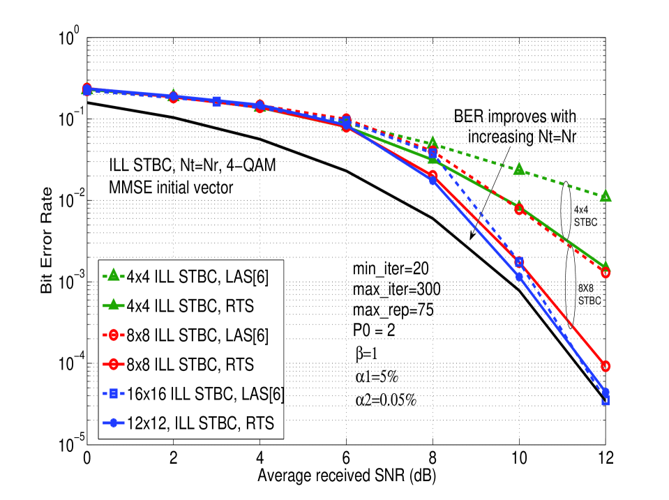
RTS versus LAS Performance: In Fig. 1, we plot the uncoded BER of the RTS algorithm as a function of average received SNR per receive antenna, [15], in decoding (32 dimensions), (128 dimensions) and (288 dimensions) non-orthogonal ILL STBCs for 4-QAM and . Perfect CSIR and i.i.d fading are assumed. For the same settings, performance of the LAS algorithm in [4]-[6] are also plotted for comparison. MMSE initial vector is used in both RTS and LAS. As a reference, we have plotted the BER performance on a SISO AWGN channel as well. From Fig. 1, the following interesting observations can be made:
-
•
the BER of RTS algorithm improves and approaches SISO AWGN performance as (i.e., STBC size) is increased; e.g., performance close to within 0.5 dB from SISO AWGN performance is achieved at uncoded BER in decoding STBC with 288 real dimensions.
-
•
RTS algorithm performs better than LAS algorithm (see RTS and LAS BER plots for and STBCs. Further, while both RTS and LAS algorithms exhibit large system behavior (i.e., BER improves as is increased), RTS is able to achieve nearness to SISO AWGN performance at BER with less number of dimensions than with LAS. This is evident by observing that, while LAS requires 512 dimensions ( STBC) to achieve 1 dB closeness to SISO AWGN performance at BER, RTS is able to achieve even 0.5 dB closeness with just 288 dimensions ( STBC). RTS is able to achieve this better performance because, while the bit/symbol-flipping strategies are similar in both RTS and LAS, the inherent escape strategy in RTS allows it to move out of local minimas and move towards better solutions. Consequently, RTS incurs some extra complexity compared to LAS, without increase in the order of complexity.
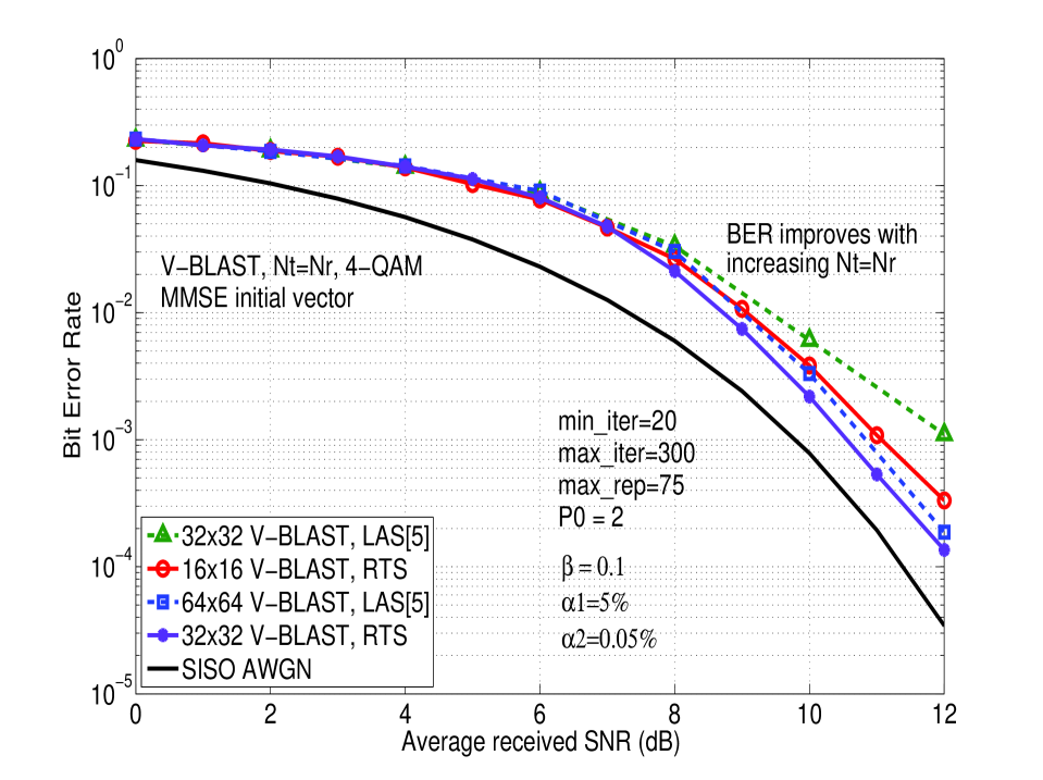
RTS performance in V-BLAST: A similar observation can be made with uncoded BER of RTS detection in V-BLAST in Fig. 2 for and 4-QAM. From Fig. 2, it is seen that LAS requires 128 dimensions ( V-BLAST) to achieve performance within 1 dB of SISO AWGN performance at BER, whereas RTS is able to achieve even better closeness with just 64 dimensions ( V-BLAST). In summary, the ability to achieve near SISO AWGN performance at less dimensions than LAS is an attractive feature of RTS.
IV-B Turbo coded BER performance of RTS
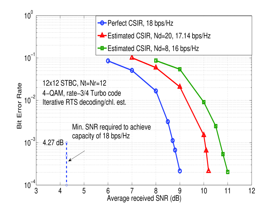
Figure 3 shows the rate-3/4 turbo coded BER of RTS decoding of non-orthogonal ILL STBC with and 4-QAM (corresponding to a spectral efficiency of 18 bps/Hz), under perfect CSIR and i.i.d fading. The theoretical minimum SNR required to achieve 18 bps/Hz spectral efficiency on a MIMO channel with perfect CSIR and i.i.d fading is 4.27 dB (obtained through simulation of the ergodic capacity formula [15]). From Fig. 3, it is seen that RTS decoding is able to achieve vertical fall in coded BER close to within about 5 dB from the theoretical minimum SNR, which is good nearness to capacity performance. This nearness to capacity can be further improved by 1 to 1.5 dB if soft decision values, proposed in [5], are fed to the turbo decoder.
IV-C Iterative RTS Decoding/Channel Estimation
Next, we relax the perfect CSIR assumption by considering a training based iterative RTS decoding/channel estimation scheme. Transmission is carried out in frames, where one pilot matrix (for training purposes) followed by data STBC matrices are sent in each frame as shown in Fig. 4. One frame length, , (taken to be the channel coherence time) is channel uses. The proposed scheme works as follows: obtain an MMSE estimate of the channel matrix during the pilot phase, use the estimated channel matrix to decode the data STBC matrices using RTS algorithm, and iterate between channel estimation and RTS decoding for a certain number of times. For ILL STBC, in addition to perfect CSIR performance, Fig. 3 also shows the performance with CSIR estimated using the above iterative RTS decoding/channel estimation scheme for and . 2 iterations between RTS decoding and channel estimation are used. With (which corresponds to large coherence times, i.e., slow fading) the BER and bps/Hz with estimated CSIR get closer to those with perfect CSIR.
IV-D Effect of MIMO Spatial Correlation
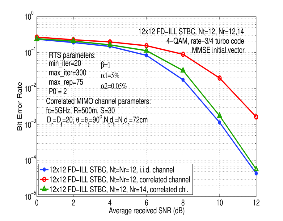
In Figs. 1 to 3, we assumed i.i.d fading. But spatial correlation at transmit/receive antennas and the structure of scattering and propagation environment can affect the rank structure of the MIMO channel resulting in degraded performance [16],[17]. We relaxed the i.i.d. fading assumption by considering the correlated MIMO channel model proposed by Gesbert et al in [17], which takes into account carrier frequency (), spacing between antenna elements (), distance between tx and rx antennas (), and scattering environment. In Fig. 5, we plot the uncoded BER of RTS decoding of FD-ILL STBC with perfect CSIR in i.i.d. fading, and correlated MIMO fading model in [17]. It is seen that, compared to i.i.d fading, there is a loss in diversity order in spatial correlation for ; further, use of more receive antennas () alleviates this loss in performance. Finally, we note that have carried out simulations of RTS decoding for 16-QAM as well, where similar results reported here for 4-QAM are observed. The RTS decoding can be used to decode perfect codes of large dimensions as well.
References
- [1] B. A. Sethuraman, B. Sundar Rajan, and V. Shashidhar, “Full-diversity high-rate space-time block codes from division algebras,” IEEE Trans. Inform. Theory, vol. 49, no. 10, pp. 2596-2616, October 2003.
- [2] F. Oggier, J.-C. Belfiore, and E. Viterbo, Cyclic Division Algebras: A Tool for Space-Time Coding, Foundations and Trends in Commun. and Inform. Theory, vol. 4, no. 1, pp. 1-95, Now Publishers, 2007.
- [3] J.-C. Belfiore, G. Rekaya, and E. Viterbo, “The golden code: A full-rate space-time code with non-vanishing determinants,” IEEE Trans. Inform. Theory, vol. 51, no. 4, April 2005.
- [4] K. Vishnu Vardhan, Saif K. Mohammed, A. Chockalingam, B. Sundar Rajan, “A low-complexity detector for large MIMO systems and multicarrier CDMA systems,” IEEE JSAC Spl. Iss. on Multiuser Detection, for Adv. Commun. Systems and Networks, pp. 473-485, April 2008.
- [5] Saif K. Mohammed, A. Chockalingam, and B. Sundar Rajan, “A low-complexity near-ML performance achieving algorithm for large MIMO detection,” Proc. IEEE ISIT’2008, Toronto, July 2008.
- [6] Saif K. Mohammed, A. Chockalingam, and B. Sundar Rajan, “High-rate space-time coded large MIMO systems: Low-complexity detection and performance,” Proc. IEEE GLOBECOM’2008, December 2008.
- [7] http://www.ruckuswireless.com/technology/beamflex.php
- [8] F. Glover, “Tabu Search - Part I,” ORSA Journal of Computing, vol. 1, no. 3, Summer 1989, pp. 190-206.
- [9] F. Glover, “Tabu Search - Part II,” ORSA Journal of Computing, vol. 2, no. 1, Winter 1990, pp. 4-32.
- [10] F. Glover and M. Laguna, “Tabu Search - Modern Heuristic Techniques for Combinatorial Problems,” Colin R. Reeves Ed., 70-150, Blackwell Scientific Publications, Oxford, 1993.
- [11] R. Battiti and G. Tecchiolli, “The reactive tabu search,” ORSA Journal on Computing, no. 2, pp. 126-140, 1994.
- [12] Y. Huang and J. A. Ritcey, “Improved 16-QAM constellation labeling for BI-STCM-ID with the Alamouti scheme,” IEEE Commun. Letters, vol. 9, no. 2, pp. 157-159, February 2005.
- [13] P. H. Tan and L. K. Rasmussen, “Multiuser detection in CDMA - A comparison of relaxations, exact, and heuristic search methods,” IEEE Trans. Wireless Commun., pp. 1802-1809, September 2004.
- [14] H. Zhao, H. Long, and W. Wang, “Tabu search detection for MIMO systems,” Proc. IEEE PIMRC’2007, Athens, September 2007.
- [15] H. Jafarkhani, Space-Time Coding: Theory and Practice, Cambridge University Press, 2005.
- [16] D. Shiu, G. J. Foschini, M. J. Gans, and J. M. Khan, “Fading correlation and its effect on the capacity of multi-antenna systems,” IEEE Trans. on Commun., vol. 48, pp. 502-513, March 2000.
- [17] D. Gesbert, H. Bölcskei, D. A. Gore, and A. J. Paulraj, “Outdoor MIMO wireless channels: Models and performance prediction,” IEEE Trans. on Commun., vol. 50, pp. 1926-1934, December 2002.