Low-Rank Covariance Function Estimation for Multidimensional Functional Data
Abstract
Multidimensional function data arise from many fields nowadays. The covariance function plays an important role in the analysis of such increasingly common data. In this paper, we propose a novel nonparametric covariance function estimation approach under the framework of reproducing kernel Hilbert spaces (RKHS) that can handle both sparse and dense functional data. We extend multilinear rank structures for (finite-dimensional) tensors to functions, which allow for flexible modeling of both covariance operators and marginal structures. The proposed framework can guarantee that the resulting estimator is automatically semi-positive definite, and can incorporate various spectral regularizations. The trace-norm regularization in particular can promote low ranks for both covariance operator and marginal structures. Despite the lack of a closed form, under mild assumptions, the proposed estimator can achieve unified theoretical results that hold for any relative magnitudes between the sample size and the number of observations per sample field, and the rate of convergence reveals the “phase-transition” phenomenon from sparse to dense functional data. Based on a new representer theorem, an ADMM algorithm is developed for the trace-norm regularization. The appealing numerical performance of the proposed estimator is demonstrated by a simulation study and the analysis of a dataset from the Argo project.
Keywords: Functional data analysis; multilinear ranks; tensor product space; unified theory
1 Introduction
In recent decades, functional data analysis (FDA) has become a popular branch of statistical research. General introductions to FDA can be found in a few monographs (e.g., Ramsay and Silverman, 2005; Ferraty and Vieu, 2006; Horváth and Kokoszka, 2012; Hsing and Eubank, 2015; Kokoszka and Reimherr, 2017). While traditional FDA deals with a sample of time-varying trajectories, many new forms of functional data have emerged due to improved capabilities of data recording and storage, as well as advances in scientific computing. One particular new form of functional data is multidimensional functional data, which becomes increasingly common in various fields such as climate science, neuroscience and chemometrics. Multidimensional functional data are generated from random fields, i.e., random functions of several input variables. One example is multi-subject magnetic resonance imaging (MRI) scans, such as those collected by the Alzheimer’s Disease Neuroimaging Initiative. A human brain is virtually divided into three-dimensional boxes called “voxels” and brain signals obtained from these voxels form a three-dimensional functional sample indexed by spatial locations of the voxels. Despite the growing popularity of multidimensional functional data, statistical methods for such data are limited apart from very few existing works (e.g., Huang et al., 2009; Allen, 2013; Zhang et al., 2013; Zhou and Pan, 2014; Wang and Huang, 2017).
In FDA covariance function estimation plays an important role. Many methods have been proposed for unidimensional functional data (e.g., Rice and Silverman, 1991; James et al., 2000; Yao et al., 2005; Paul and Peng, 2009; Li and Hsing, 2010; Goldsmith et al., 2011; Xiao et al., 2013), and a few were particularly developed for two-dimensional functional data (e.g., Zhou and Pan, 2014; Wang and Huang, 2017). In general when the input domain is of dimension , one needs to estimate a -dimensional covariance function. Since covariance function estimation in FDA is typically nonparametric, the curse of dimensionality emerges soon when is moderate or large.
For general , most work are restricted to regular and fixed designs (e.g., Zipunnikov et al., 2011; Allen, 2013), where all random fields are observed over a regular grid like MRI scans. Such sampling plan leads to a tensor dataset, so one may apply tensor/matrix decompositions to estimate the covariance function. When random fields are observed at irregular locations, the dataset is no longer a completely observed tensor so tensor/matrix decompositions are not directly applicable. If observations are densely collected for each random field, a two-step approach is a natural solution, which involves pre-smoothing every random field followed by ensor/matrix decompositions at a fine discretized grid. However, this solution is infeasible for sparse data where there are a limited number of observations per random field. One example is the data collected by the international Argo project (http://www.argo.net). See Section 7 for more details. In such sparse data setting, one may apply the local smoothing method of Chen and Jiang (2017), but it suffers from the curse of dimensionality when the dimension is moderate due to a -dimensional nonparametric regression.
We notice that there is a related class of literature on longitudinal functional data (e.g., Chen and Müller, 2012; Park and Staicu, 2015; Chen et al., 2017), a special type of multidimensional functional data where a function is repeatedly measured over longitudinal times. Typically multi-step methods are needed to model the functional and longitudinal dimensions either separately (one dimension at a time) or sequentially (one dimension given the other), as opposed to the joint estimation procedure proposed in this paper. We also notice a recent work on longitudinal functional data under the Bayesian framework (Shamshoian et al., 2019).
The contribution of this paper is three-fold. First, we propose a new and flexible nonparametric method for low-rank covariance function estimation for multidimensional functional data, via the introduction of (infinite-dimensional) unfolding operators (See Section 3). This method can handle both sparse and dense functional data, and can achieve joint structural reductions in all dimensions, in addition to rank reduction of the covariance operator. The proposed estimator is guaranteed to be semi-positive definite. As a one-step procedure, our method reduces the theoretical complexities compared to multi-steps estimators which often involve a functional principal component analysis followed by a truncation and reconstruction step (e.g., Hall and Vial, 2006; Poskitt and Sengarapillai, 2013).
Second, we generalize the representer theorem for unidimensional functional data by Wong and Zhang (2019) to the multidimensional case with more complex spectral regularizations. The new representer theorem makes the estimation procedure practically computable by generating a finite-dimensional parametrization to the solution of the underlying infinite-dimensional optimization.
Finally, a unified asymptotic theory is developed for the proposed estimator. It automatically incorporates the settings of dense and sparse functional data, and reveals a phase transition in the rate of convergence. Different from existing theoretical work heavily based on closed-form representations of estimators, (Li and Hsing, 2010; Cai and Yuan, 2010; Zhang and Wang, 2016; Liebl, 2019), this paper provides the first unified theory for penalized global M-estimators of covariance functions which does not require a closed-form solution. Furthermore, a near-optimal (i.e., optimal up to a logarithmic order) one-dimensional nonparametric rate of convergence is attainable for the -dimensional covariance function estimator for Sobolev-Hilbert spaces.
The rest of the paper is organized as follows. Section 2 provides some background on reproducing kernel Hilbert space (RKHS) frameworks for functional data. Section 3 introduces Tucker decomposition for finite-dimensional tensors and our proposed generalization to tensor product RKHS operators, which is the foundation for our estimation procedure. The proposed estimation method is given in Section 4, together with an computational algorithm. The unified theoretical results are presented in Section 5. The numerical performance of the proposed method is evaluated by a simulation study in Section 6 and a real data application in Section 7.
2 RKHS Framework for Functional Data
In recent years there is a surge of RKHS methods in FDA (e.g., Yuan and Cai, 2010; Zhu et al., 2014; Li and Song, 2017; Reimherr et al., 2018; Sun et al., 2018; Wong et al., 2019). However, covariance function estimation, a seemingly well-studied problem, does not receive the same amount of attention in the development of RKHS methods, even for unidimensional functional data. Interestingly, we find that the RKHS modeling provides a versatile framework for both unidimensional and multidimensional functional data.
Let be a random field defined on an index set , with a mean function and a covariance function , and let be independently and identically distributed (i.i.d.) copies of . Typically, a functional dataset is represented by , where
| (1) |
is the noisy measurement of the -th random field taken at the corresponding index , is the number of measurements observed from the -th random field, and are independent errors with mean zero and finite variance. For simplicity and without loss of generality, we assume for all .
As in many nonparametric regression setups such as penalized regression splines (e.g., Pearce and Wand, 2006) and smoothing splines (e.g., Wahba, 1990; Gu, 2013), the sample field of , i.e., the realized (as opposed to the sample path of a unidimensional random function), is assumed to reside in an RKHS of functions defined on with a continuous and square integrable reproducing kernel . Let and denote the inner product and norm of respectively. With the technical condition , the covariance function resides in the tensor product RKHS . It can be shown that is an RKHS, equipped with the reproducing kernel defined as , for any . This result has been exploited by Cai and Yuan (2010) and Wong and Zhang (2019) for covariance estimation in the unidimensional setting.
For any function , there exists an operator mapping to defined by . When is a covariance function, we call the induced operator a -covariance operator, or simply a covariance operator as below. To avoid clutter, the induced operator will share the same notation with the generating function. Similar to -covariance operators, the definition of an induced operator is obtained by replacing the inner product by the RKHS inner product. The benefits of considering this operator have been discussed in Wong and Zhang (2019). We also note that a singular value decomposition (e.g., Hsing and Eubank, 2015) of the induced operator exists whenever the corresponding function belongs to the tensor product RKHS . The idea of induced operator can be similarly extended to general tensor product space where and are two generic RKHSs of functions.
For any , let be the transpose of , i.e., , . Define . To guarantee symmetry and positive semi-definiteness of the estimators, Wong and Zhang (2019) adopted as the hypothesis class of and considered the following regularized estimator:
| (2) |
where is a convex and smooth loss function characterizing the fidelity to the data, is a spectral penalty function (see Definition 5 below), and is a tuning parameter. Due to the constraints specified in , the resulting covariance estimator is always positive semi-definite. In particular, if the spectral penalty function imposes the trace-norm regularization, an -type shrinkage penalty on the respective singular values, the estimator is usually of low rank. Cai and Yuan (2010) adopted a similar objective function as in (2) but with the hypothesis class and an -type penalty , so the resulting estimator may neither be positive semi-definite nor low-rank.
Although Cai and Yuan (2010) and Wong and Zhang (2019) focused on unidimensional functional data, their frameworks can be directly extended to the multidimensional setting. Explicitly, similar to (2), as long as a proper for the random fields with dimension is selected, an efficient “one-step” covariance function estimation with the hypothesis class can be obtained immediately, which results in a positive semi-definite and possibly low-rank estimator. Since an RKHS is identified by its reproducing kernel, we simply need to pick a multivariate reproducing kernel for multidimensional functional data. However, even when the low-rank approximation/estimation is adopted (e.g., by trace-norm regularization), we still need to estimate several -dimensional eigenfunctions nonparametrically. This curse of dimensionality calls for a more efficient modeling. Below, we explore this through the lens of tensor decomposition in finite-dimensional vector spaces and its extension to infinite-dimensional function spaces.
3 Low-Rank Modeling via Functional Unfolding
In this section we will extend the well-known Tucker decomposition for finite-dimensional tensors to functional data, then introduce the concept of functional unfolding for low-rank modeling, and finally apply functional unfolding to covariance function estimation.
3.1 Tucker decomposition for finite-dimensional tensors
First, we give a brief introduction to the popular Tucker decomposition (Tucker, 1966) for finite-dimensional tensors. Let denote a generic tensor product space with finite-dimensional . If the dimension of is , , then each element in can be identified by an array in , which contains the coefficients through an orthonormal basis. By Tucker decomposition, any array in can be represented in terms of -mode products as follows.
Definition 1 (-mode product).
For any arrays and ,
, the -mode product between and , denoted by , is a array of dimension
of which -th element is defined by
Definition 2 (Tucker decomposition).
Tucker decomposition of is
| (3) |
where , are called the “factor matrices” (usually orthonormal) with and is called the “core tensor”.
Figure 1 provides a pictorial illustration of a Tucker decomposition. Unlike matrices, the concept of rank is more complicated for arrays of order 3 or above. Tucker decomposition naturally leads to a particular form of rank, called “multilinear rank”, which is directly related to the familiar concept of matrix ranks. To see this, we employ a reshaping operation called matricization, which rearranges elements of an array into a matrix.
=
Definition 3 (Matricization).
For any , the -mode matricization of , denoted by , is a matrix of dimension of which -th element is defined by , where 111All empty products are defined as 1. For example, when ..
For any , by simple derivations, one can obtain a useful relationship between the -mode matricization and Tucker decomposition :
| (4) |
where, with a slight abuse of notation, also represents the Kronecker product between matrices. Hence if the factor matrices are of full rank, then . The vector is known as the multilinear rank of . Clearly from (4), one can choose a Tucker decomposition such that are orthonormal matrices and . Therefore a “small” multilinear rank corresponds to a small core tensor and thus an intrinsic dimension reduction, which potentially improves estimation and interpretation. We will relate this low-rank structure to multidimensional functional data.
3.2 Functional unfolding for infinite-dimensional tensors
To encourage low-rank structures in covariance function estimation, we generalize the matricization operation for finite-dimensional arrays to infinite-dimensional tensors (Hackbusch, 2012). Here let denote a generic tensor product space where is an RKHS of functions with an inner product , for .
Notice that the tensor product space can be generated by some elementary tensors of the form where . More specifically, is the completion of the linear span of all elementary tensors under the inner product , for any .
In Definition 4 below, we generalize matricization/unfolding for finite-dimensional arrays to infinite-dimensional elementary tensors. We also define a square unfolding for infinite-dimensional tensors that will be used to describe the spectrum of covariance operators.
Definition 4 (Functional unfolding operators).
The one-way unfolding operator and square unfolding operators are defined as follows for any elementary tensor of the form .
-
1.
One-way unfolding operator for : The -mode one-way unfolding operator is defined by .
-
2.
Square unfolding operator : When is even, the square unfolding operator is defined by .
These definitions extend to any function by linearity. For notational simplicity we denote by , , and by .
Note that the range of each functional unfolding operator, either , or , is a tensor product of two RKHSs, so its output can be interpreted as an (induced) operator. Given a function , the multilinear rank can be defined as , where ’s are interpreted as an operator here and is the rank of any operator . If all are finite-dimensional, the singular values of the output of any functional unfolding operator match with those of the -mode matricization (of the corresponding array representation).
3.3 Functional unfolding for covariance functions
Suppose that the random field where each is a RKHS of functions equipped with an inner product and corresponding norm , . Then the covariance function resides in . To estimate , we could consider a special case of in Section 3.2 by letting , for ; for ; and for .
Clearly, the elements of are identified by those in . In terms of the folding structure, has a squarely unfolded structure. Since a low-multilinear-rank structure is represented by different unfolded forms, it would be easier to study the completely folded space instead of the squarely unfolded space . We use to represent the folded covariance function, the corresponding element of in . In other words, . For any , is defined as the two-way rank of while are defined as the one-way ranks of .
Remark 1.
For an array , the one-way unfolding is the same as matricization, if we further impose the same ordering of the columns in the output of , . This ordering is just related to how we represent the array, and is not crucial in the general definition of . Since the description of the computation strategy depends on the explicit representation, we will always assume this ordering. Similarly, we also define a specific ordering of rows and columns for when is even, such that its -th entry is where and .
3.4 One-way and two-way ranks in covariance functions
Here we illustrate the roles of one-way and two-way ranks in the modeling of covariance functions. For a general , let be a set of orthonormal basis functions of for , where is allowed to be infinite, depending on the dimensionality of . Then forms a set of orthonormal basis functions for . Thus for any , we can express
| (5) |
where the coefficients are real numbers. For convenience, we collectively put them into an array .
To illustrate the low-multilinear-rank structures for covariance functions, we consider , i.e., , and then by (5) the folded covariance function can be expressed by
To be precise, the covariance function is the squarely unfolded . Suppose that possesses (or is well-approximated by) a structure of a low multilinear rank, and yields Tucker decomposition 222Definition 1 is extended to the case when is infinite. where , for , and columns of are orthonormal. Apparently is the two-way rank of , while and are the corresponding one-way ranks. Now the covariance function can be further represented as
where and are (possibly infinite) linear combinations of the original basis functions. In fact, and are the sets of orthonormal functions of and respectively. Apparently .
Consider the eigen-decomposition of the squarely unfolded core tensor where and has orthonormal columns. Then we obtain the eigen-decomposition of the covariance function :
where the eigenfunction is
with and .
First, this indicates that the two-way rank is the same as the rank of the covariance operator. Second, this shows that is the common basis for the variation along the dimension , hence describing the marginal structure along . Similarly is the common basis that characterizes the marginal variation along the dimension . We call them the marginal basis along the respective dimension. Therefore, the one-way ranks and are the minimal numbers of the one-dimensional functions for the dimensions and respectively that construct all the eigenfunctions of covariance function .
Similarly, for -dimensional functional data, each eigenfunction can be represented by a linear combination of -products of univariate functions. One can then show that the two-way rank is the same as the rank of the covariance operator and the one-way ranks are the minimal numbers of one-dimensional functions along respective dimensions that characterize all eigenfunctions of the covariance operator.
Remark 2.
Obviously, for -dimensional functional data. If the random field has the property of “weak separability” as defined by Lynch and Chen (2018), then so the low-rank structure in terms of will be automatically translated to low one-way ranks. Note that the construction of our estimator and corresponding theoretical analysis do not require separability conditions.
Compared to typical low-rank covariance modelings only in terms of , we also intend to regularize the one-way ranks for two reasons. First, the illustration above shows that the structure of low one-way ranks encourages a “sharing” structure of one-dimensional variations among different eigenfunctions. Promoting low one-way ranks can facilitate additional dimension reduction and further alleviates the curse of dimensionality. Moreover, one-dimensional marginal structures will provide more details of the covariance function structure and thus help with a better understanding of -dimensional eigenfunctions.
Therefore, we will utilize both one-way and two-way structures and propose an estimation procedure that regularizes one-way and two-way ranks jointly and flexibly, with the aim of seeking the “sharing” of marginal structures while controlling the number of eigen-components simultaneously.
4 Covariance Function Estimation
In this section we propose a low-rank covariance function estimation framework based on functional unfolding operators and spectral regularizations. Spectral penalty functions (Abernethy et al., 2009; Wong and Zhang, 2019) are defined as follows.
Definition 5 (Spectral penalty function).
Given a compact operator , a spectral penalty function takes the form with the singular values of the operator , , , in a descending order of magnitude and a non-decreasing penalty function such that .
Recall and where , for , and for . Clearly, a covariance operator is self-adjoint and positive semi-definite. Therefore we consider the hypothesis space , where , and propose a general class of covariance function estimators as follows:
| (6) |
where is a convex and smooth loss function, are spectral penalty functions, and , are tuning parameters. Here penalizes the squarely unfolded operator while regularizes one-way unfolded operator respectively for . The tuning parameter controls the relative degree of regularization between one-way and two-way singular values. The larger the is, the more penalty is imposed on the two-way singular values relative to the one-way singular values. When , the penalization is only on the eigenvalues of the covariance operator (i.e., the two-way singular values), similarly as Wong and Zhang (2019).
To achieve low-rank estimation, we adopt a special form of (6):
| (7) |
where is the sum of singular values, also called trace norm, and is the squared error loss:
| (8) |
with , as an estimate of the mean function, and as the -th element of location vector . Notice that trace-norm regularizations promote low-rankness of the underlying operators, hence leading to a low-rank estimation in terms of both the one-way and two-way (covariance) ranks.
4.1 Representer theorem and parametrization
Before deriving a computational algorithm, we notice that the optimization (7) is an infinite-dimensional optimization which is generally unsolvable. To overcome this challenge, we show that the solution to (7) always lies in a known finite-dimensional sub-space given data, hence allowing a finite-dimensional parametrization. Indeed, we are able to achieve a stronger result in Theorem 1 which holds for the general class of estimators obtained by (6).
Let .
Theorem 1 (Representer theorem).
If the solution set of (6) is not empty, there always exists a solution lying in the space , where and
for .
The solution takes the form:
| (9) |
where the -th element of is with . Also, is a -th order tensor where the dimension of each mode is and is a symmetric matrix.
The proof of Theorem 1 is given in Section S1 of the supplementary material. By Theorem 1, we can now only focus on covariance function estimators of the form (9). Let , where is a matrix such that . With , we can express
| (10) | ||||
where is defined in Theorem 1 and is the Moore–Penrose inverse of matrix .
The Gram matrix is often approximately low-rank. For computational simplicity, one could adopt to be significantly smaller than . Ideally we can obtain the “best” low-rank approximation with respect to the Frobenius norm by eigen-decomposition, but a full eigen-decomposition is computationally expensive. Instead, randomized algorithms can be used to obtain low-rank approximations in an efficient manner (Halko et al., 2009).
One can easily show that the eigenvalues of the operator are the same as those of the matrix and that the singular values of the operator are the same as those of the matrix . Therefore, solving (7) is equivalent to solving the following optimization:
| (11) |
where also represents the trace norm of matrices, if matrix is positive semi-definite, and otherwise, and , where is constructed from (10).
Beyond estimating the covariance function, one may be further interested in the eigen-decomposition of via the inner product, e.g., to perform functional principal component analysis in the usual sense. Due to the finite-dimensional parametrization, a closed-form expression of eigen-decomposition can be derived from our estimator without further discretization or approximation. In addition, we can obtain a similar one-way analysis in terms of the inner product. We can define a singular value decomposition via the Tucker form and obtain the marginal basis. Details are given in Appendix A.
4.2 Computational algorithm
We solve (11) by the accelerated alternating direction method of multipliers (ADMM) algorithm (Kadkhodaie et al., 2015). We begin with an alternative form of (11):
| (12) | ||||
| (13) |
where for .
Then a standard ADMM algorithm solves the optimization problem (12) by minimizing the augmented Lagrangian with respect to different variables alternatively. More explicitly, at the -th iteration, the following updates are implemented:
| (14a) | ||||
| (14b) | ||||
| (14c) | ||||
| (14d) | ||||
where , for , are scaled Lagrangian multipliers and is an algorithmic parameter. An adaptive strategy to tune is provided in Boyd et al. (2010). One can see that Steps (14a), (14b) and (14c) involve additional optimizations. Now we discuss how to solve them.
The objective function of (14a) is a quadratic function, and so we can easily solve this with a closed-form solution, given in line 2 of Algorithm 1. To solve (14b) and (14c), we use proximal operator , and respectively defined by
| (15a) | ||||
| (15b) | ||||
for . By Lemma 1 in Mazumder et al. (2010), the solutions to (15) have closed forms.
For (15a), write the singular value decomposition of as , then where . As for (15b), is restricted to be a symmetric matrix since the penalty equals infinity otherwise. Thus (15b) is equivalent to minimizing since . Suppose that yields eigen-decomposition . Then , where . Unlike singular values, the eigenvalues may be negative. Hence, as opposed to , this procedure also removes eigen-components with negative eigenvalues.
The details of computational algorithm are given in Algorithm 1, an accelerated version of ADMM which involves additional steps for a faster algorithmic convergence.
5 Asymptotic Properties
In this section, we conduct an asymptotic analysis for the proposed estimator as defined in (7). Our analysis has a unified flavor such that the derived convergence rate of the proposed estimator automatically adapts to sparse and dense settings. Throughout this section, we neglect the mean function estimation error by setting for any , which leads to a cleaner and more focused analysis. The additional error from the mean function estimation can be incorporated into our proofs without any fundamental difficulty.
5.1 Assumptions
Without loss of generality let . The assumptions needed in the asymptotic results are listed as follows.
Assumption 1.
Sample fields reside in where is an RKHS of functions on with a continuous and square integrable reproducing kernel .
Assumption 2.
The true (folded) covariance function and , where , for and for .
Assumption 3.
The locations
are independent
random vectors from ,
and they are independent of
.
The errors are independent of both locations and sample fields.
Assumption 4.
For each , is sub-Gaussian with a parameter which does not depend on , i.e., for all and .
Assumption 5.
For each and , is a mean-zero sub-Gaussian random variable with a parameter independent of and , i.e., .
Moreover
all errors are independent.
Assumption 1 delineates a tensor product RKHS modeling, commonly seen in the nonparametric regression literature (e.g., Wahba, 1990; Gu, 2013). In Assumption 2, the condition is satisfied if , as shown in Cai and Yuan (2010). Assumption 3 is specified for random design and we adopt the uniform distribution here for simplicity. The uniform distribution on can be generalized to any other continuous distribution of which density function satisfies for all , for some constants , to ensure both Theorems 2 and 3 still hold. Assumptions 4 and 5 involve sub-Gaussian conditions of the stochastic process and measurement error, which are standard tail conditions.
5.2 Reproducing kernels
In Assumption 1, the “smoothness” of the function in the underlying RKHS is not explicitly specified. It is well-known that such smoothness conditions are directly related to the eigen-decay of the respective reproducing kernel. By Mercer’s Theorem (Mercer, 1909), the reproducing kernel of possesses the eigen-decomposition
| (16) |
where are non-negative eigenvalues and are eigenfunctions on . Then for the space , which is also identified by , its corresponding reproducing kernel has the following eigen-decomposition
where are the eigenvalues of . Due to continuity assumption (Assumption 1) of the univariate kernels, there exists a constant such that
The decay rate of the eigenvalues is involved in our analysis through two quantities and , which have relatively complex forms defined in Appendix B. Similar quantities can be found in other analyses of RKHS-based estimators (e.g., Raskutti et al., 2012) that accommodate general choices of RKHS. Generally and are expected to diminish in certain orders of and , characterized by the decay rate of the eigenvalues . The smoother the functions in the RKHS, the faster these two quantities diminish. Our general results in Theorems 2 and 3 are specified in terms of these quantities. To provide a solid example, we derive the orders of and under a Sobolev-Hilbert space setting and provide the convergence rate of the proposed estimator in Corollary 1.
5.3 Unified rates of convergence
We write the penalty in (7) as . For arbitrary functions , define their empirical inner product and the corresponding (squared) empirical norm as
Additionally, the norm of a function is defined as .
Define . We first provide the empirical rate of convergence for .
Theorem 2.
Next, we provide the rate of convergence for .
Theorem 3.
Under the same conditions as Theorem 2, there exist a positive constant depending on , , and , such that
with probability at least for some constant depending on .
Remark 3.
Theorems 2 and 3 are applicable to general RKHS which satisfies Assumption 1. The convergence rate depends on the eigen-decay rates of the reproducing kernel. A special case of polynomial decay rates for univariate RKHS will be given in Corollary 1. Moreover, our analysis has a unified flavor in the sense that the resulting convergence rates automatically adapt to the orders of both and . In Remark 5 we will provide a discussion of a “phase transition” between dense and sparse functional data revealed by our theory.
Remark 4.
With a properly chosen , Theorems 2 and 3 bound the convergence rates (in terms of both the empirical and theoretical norm) by , which cannot be faster than . The logarithmic order is due to the use of Adamczak bound in Lemma S2 in the supplementary material. If one further assumes boundedness for the sample fields ’s (in terms of the sup-norm) and the noise variables ’s, we can instead use Talagrand concentration inequality (Bousquet bound in Koltchinskii (2011)) and the results in Theorems 2 and 3 can be improved to , where .
Next we focus on a special case where the reproducing kernels of the univariate RKHS ’s exhibit polynomial eigen-decay rates, which holds for a range of commonly used RKHS. A canonical example is -th order Sobolev-Hilbert space:
where . Here is the same as in Corollary 1. To derive the convergence rates, we relate the eigenvalues in (16) to the univariate RKHS , . Due to Mercer’s Theorem, the reproducing kernel of yields an eigen-decomposition with non-negative eigenvalues and an eigenfunction , i.e., Therefore, the set of eigenvalues in (16) is the same as the set . Given the eigen-decay of , one can obtain the order of and hence the convergence rates from Theorems 2 and 3. Here are the results under the setting of a polynomial eigen-decay.
Corollary 1.
Suppose that the same conditions in Theorem 3 hold. If the eigenvalues of for have polynomial decaying rates, that is, there exists such that for all , then
Remark 5.
All Theorems 2 and 3 and Corollary 1 reveal a “phase-transition” of the convergence rate depending on the relative magnitudes between , the sample size, and , the number of observations per field. When , which is equivalent to in Corollary 1, both empirical and theoretical rates of convergence can achieve the near-optimal rate . Under the stronger assumptions in Remark 4, the convergence rate will achieve the optimal order when (or in Corollary 1). In this case, the observations are so densely sampled that we can estimate the covariance function as precisely as if the entire sample fields are observable. On the contrary, when (or in Corollary 1), the convergence rate is determined by the total number of observations . When , the asymptotic result in Corollary 1, up to some and terms, is the same as the minimax optimal rate obtained by Cai and Yuan (2010), and is comparable to the rate obtained by Paul and Peng (2009) for .
Remark 6.
For covariance function estimation for unidimensional functional data, i.e., , a limited number of approaches, including Cai and Yuan (2010), Li and Hsing (2010), Zhang and Wang (2016), and Liebl (2019), can achieve unified theoretical results in the sense that they hold for all relative magnitudes of and . The similarity of these approaches is the availability of a closed form for each covariance function estimator. In contrast, our estimator obtained from (7) does not have a closed form due to the non-differentiability of the penalty, but it can still achieve unified theoretical results which hold for both unidimensional and multidimensional functional data. Due to the lack of a closed form of our covariance estimator, we used the empirical process techniques (e.g., Bartlett et al., 2005; Koltchinskii, 2011) in the theoretical development. In particular, we have developed a novel grouping lemma (Lemma S4 in the supplementary material) to deterministically decouple the dependence within a -statistics of order 2. We believe this lemma is of independent interest. In our analysis, the corresponding -statistics is indexed by a function class, and this grouping lemma provides a tool to obtain uniform results (see Lemma S3 in the supplementary material). In particular, this allows us to relate the empirical and theoretical norm of the underlying function class, in precise enough order dependence on and to derive the unified theory. See Lemma S3 for more details. To the best of our knowledge, this paper is one of the first in the FDA literature that derives a unified result in terms of empirical process theories, and the proof technique is potentially useful for some other estimators without a closed form.
6 Simulation
To evaluate the practical performance of the proposed method, we conducted a simulation study. We in particular focused on two-dimensional functional data. Let and both be the RKHS with kernel , where , . This RKHS has been used in various studies in FDA, e.g., the simulation study of Cai and Yuan (2012). Each is generated from a mean-zero Gaussian random field with a covariance function
where the eigenfunctions . Three combinations of one-way ranks () and two-way rank were studied for :
Setting 1: , , ; Setting 2: , ;
Setting 3: .
For each setting, we chose functions out of to be such that smoother functions are associated with larger eigenvalues. The details are described in Section S2.1 of the supplementary material.
In terms of sampling plans, we considered both sparse and dense designs. Due to the space limit, here we only show and discuss the results for the sparse design, while defer those for the dense design to Section S2.3 of the supplementary material. For the sparse design, the random locations were independently generated from the continuous uniform distribution on within each field and across different fields, and the random errors were independently generated from . In each of the 200 simulation runs, the observed data were obtained following (1) with various combinations of , and noise level .
We compared the proposed method, denoted by mOpCov, with three existing methods: 1) OpCov: the estimator based on Wong and Zhang (2019) with adaption to two dimensional case (see Section 2); 2) ll-smooth: local linear smoothing with Epanechnikov kernel; 3) ll-smooth+: the two-step estimator constructed by retaining eigen-components of ll-smoothselected by 99% fraction of variation explained (FVE), and then removing the eigen-components with negative eigenvalues. For both OpCov and mOpCov, 5-fold cross-validation was adopted to select the corresponding tuning parameters.
Table 1 show the average integrated squared error (AISE), average of estimated two-way rank (), as well as average of estimated one-way ranks () of the above covariance estimators over 200 simulated data sets in respective settings when sample size is . Corresponding results for can be found in Table S4 of the supplementary material, and they lead to similar conclusions. Obviously ll-smooth and ll-smooth+, especially ll-smooth, perform significantly worse than the other two methods in both estimation accuracy and rank reduction (if applicable). Below we only compare mOpCov and OpCov.
Regarding estimation accuracy, the proposed mOpCov has uniformly smaller AISE values than OpCov, with around improvement of AISE over OpCov in most cases under Settings 1 and 2. If the standard error (SE) of AISE is taken into account, the improvements of AISE by mOpCov are more distinguishable in Settings 1 and 2 than those in Setting 3 since the SEs of OpCov in Setting 3 are relatively high. This is due to the fact that in Setting 3, marginal basis are not shared by different two-dimensional eigenfunctions, and hence mOpCov cannot benefit from the structure sharing among eigenfunctions. Setting 3 is in fact an extreme setting we designed to challenge the proposed method.
For rank estimation, OpCov almost always underestimates two-way ranks, while mOpCov typically overestimates both one-way and two-way ranks. For mOpCov, the average one-way rank estimates are always smaller than the average two-way rank estimates, and their differences are substantial in Settings 1 and 2. This demonstrates the benefit of mOpCov of detecting structure sharing of one-dimensional basis among two-dimensional eigenfunctions.
We also tested the performance of mOpCov in the dense and regular designs, and compared it with the existing methods mentioned above together with the one by Wang and Huang (2017), which is not applicable to the sparse design. Details are given in Section S2.3 of the supplementary material, where all methods achieve similar AISE values, but mOpCov performs slightly better in estimation accuracy when the noise level is high.
| Setting | mOpCov | OpCov | ll-smooth | ll-smooth+ | |||
|---|---|---|---|---|---|---|---|
| 1 | 10 | 0.1 | AISE | 0.053 (1.97e-03) | 0.0632 (3.22e-03) | 0.652 (1.92e-01) | 0.337 (5.35e-02) |
| 8.38 | 2.94 | - | 172.70 | ||||
| , | 5.4, 5.4 | _ | _ | _ | |||
| 0.4 | AISE | 0.0547 (2.01e-03) | 0.0656 (2.72e-03) | 0.714 (2.11e-01) | 0.366 (5.96e-02) | ||
| 9.16 | 2.84 | - | 177.3 | ||||
| , | 5.34, 5.32 | _ | _ | _ | |||
| 20 | 0.1 | AISE | 0.0343 (1.46e-03) | 0.0421 (1.97e-03) | 0.297 (1.39e-02) | 0.206 (4.62e-03) | |
| 8.38 | 3.78 | - | 317.44 | ||||
| , | 5.84, 5.82 | _ | _ | _ | |||
| 0.4 | AISE | 0.0354 (1.52e-03) | 0.044 (2.21e-03) | 0.325 (1.58e-02) | 0.223 (4.94e-03) | ||
| 8.86 | 3.76 | - | 326.31 | ||||
| , | 5.83, 5.84 | _ | _ | _ | |||
| 2 | 10 | 0.1 | AISE | 0.0532 (1.98e-03) | 0.0636 (3.12e-03) | 2.33 (1.13e+00) | 0.795 (2.98e-01) |
| 8.48 | 3.02 | - | 191.175 | ||||
| , | 5.82, 5.82 | _ | _ | _ | |||
| 0.4 | AISE | 0.0548 (2.05e-03) | 0.0686 (3.53e-03) | 2.44 (1.17e+00) | 0.828 (3.04e-01) | ||
| 9.04 | 3.04 | - | 196.34 | ||||
| , | 5.71, 5.74 | _ | _ | _ | |||
| 20 | 0.1 | AISE | 0.0341 (1.43e-03) | 0.0419 (2.02e-03) | 0.301 (1.58e-02) | 0.208 (4.50e-03) | |
| 8.99 | 3.74 | - | 318.645 | ||||
| , | 5.93, 5.92 | _ | _ | _ | |||
| 0.4 | AISE | 0.0348 (1.43e-03) | 0.043 (2.22e-03) | 0.328 (1.78e-02) | 0.225 (4.74e-03) | ||
| 8.01 | 3.6 | - | 327.395 | ||||
| , | 5.94, 5.93 | _ | _ | _ | |||
| 3 | 10 | 0.1 | AISE | 0.058 (2.62e-03) | 0.0692 (5.33e-03) | 0.454 (7.28e-02) | 0.286 (2.89e-02) |
| 6.26 | 3.12 | - | 182.74 | ||||
| , | 5, 5.06 | _ | _ | _ | |||
| 0.4 | AISE | 0.0598 (2.68e-03) | 0.0733 (6.14e-03) | 0.531 (1.07e-01) | 0.323 (4.23e-02) | ||
| 6.48 | 3.2 | - | 185.82 | ||||
| , | 4.99, 5.07 | _ | _ | _ | |||
| 20 | 0.1 | AISE | 0.0422 (1.37e-03) | 0.0535 (2.64e-03) | 0.267 (5.04e-03) | 0.196 (3.59e-03) | |
| 6.29 | 4.49 | - | 332.09 | ||||
| , | 5.62, 5.69 | _ | _ | _ | |||
| 0.4 | AISE | 0.0424 (1.30e-03) | 0.0494 (2.42e-03) | 0.292 (5.30e-03) | 0.212 (3.72e-03) | ||
| 5.68 | 3.36 | - | 338.725 | ||||
| , | 5.59, 5.66 | _ | _ | _ |
7 Real Data Application
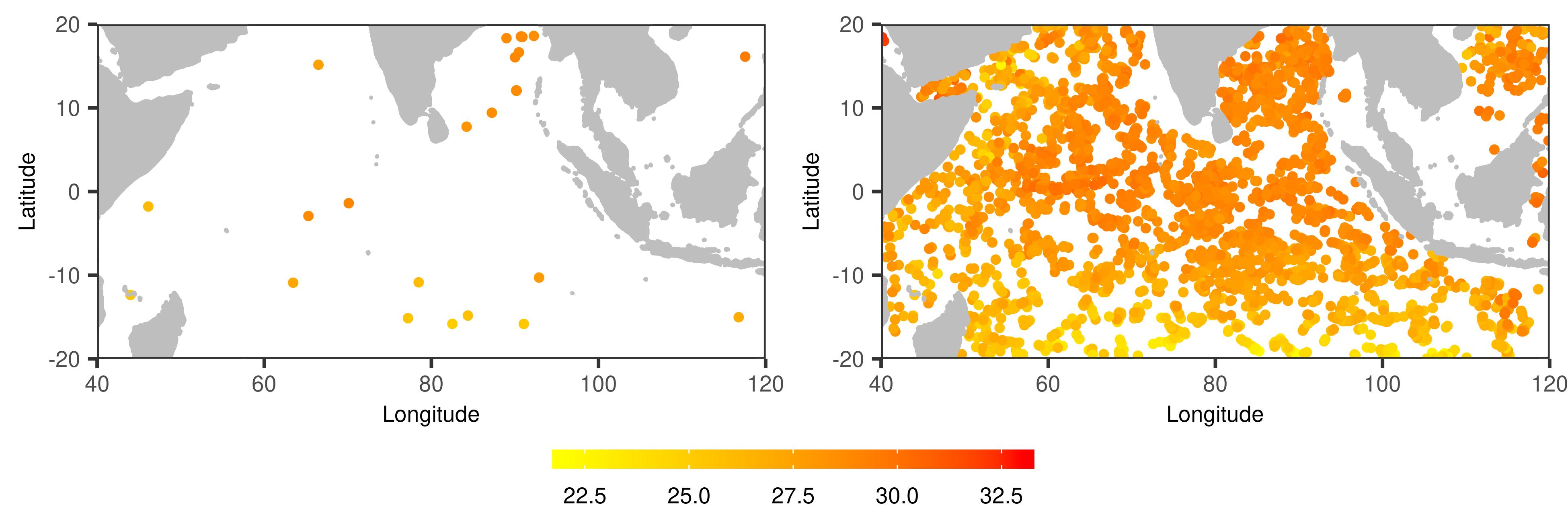
We applied the proposed method to an Argo profile data set, obtained from http://www.argo.ucsd.edu/Argo_data_and.html. The Argo project has a global array of approximately 3,800 free-drifting profiling floats, which measure temperature and salinity of the ocean. These floats drift freely in the depths of the ocean most of the time, and ascend regularly to the sea surface, where they transmit the collected data to the satellites. Every day only a small subset of floats show up on the sea surface. Due to the drifting process, these floats measure temperature and salinity at irregular locations over the ocean. See Figure 2 for examples.
In this analysis, we focus on the different changes of sea surface temperature between the tropical western and eastern Indian Ocean, which is called the Indian Ocean Dipole (IOD). The IOD is known to be associated with droughts in Australia (Ummenhofer et al., 2009) and has a significant effect on rainfall patterns in southeast Australia (Behera and Yamagata, 2003). According to Shinoda et al. (2004), the IOD phenomenon is a predominant inter-annual variation of sea surface temperature during late boreal summer and autumn (Shinoda et al., 2004), so in this application we focused on the sea surface temperature in the Indian Ocean region of longitude 40120 and latitude -2020 between September and November every year from 2003 to 2018.
Based on a simple autocorrelation analysis on the gridded data, we decided to use measurements for every ten days in order to reduce the temporal dependence among the data.
At each location of a float on a particular day, the average temperature between 0 and 5 hPa from the float is regarded as a measurement. The Argo float dataset provides multiple versions of data, and we adopted the quality controlled (QC) version. Eventually we have a two-dimensional functional data collected of days, where the number of observed locations per day varies from 7 to 47, i.e., , , with an average of 21.83. The locations are rescaled to . As shown in Figure 2, the data has a random sparse design.
First we used kernel ridge regression with the corresponding kernel for the tensor product of two second order Sobolev spaces (e.g., Wong and Zhang, 2019) to obtain a mean function estimate for every month. Then we applied the proposed covariance function estimator with the same kernel.
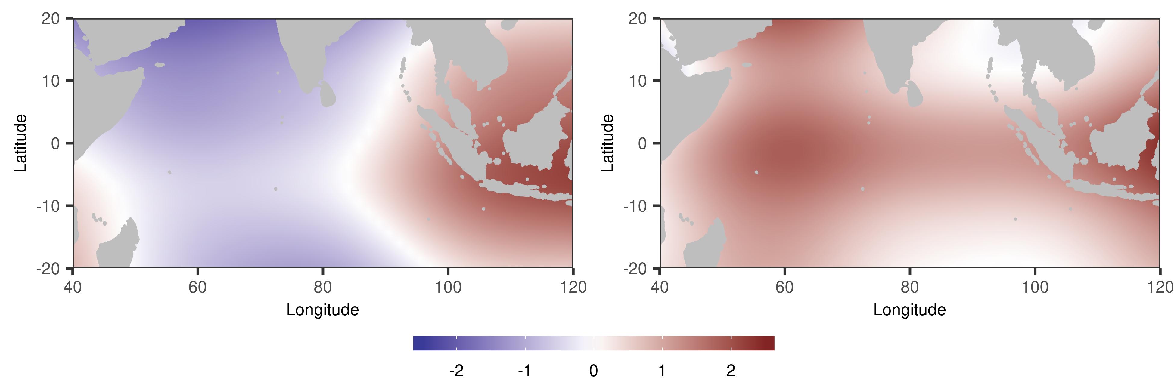
The estimates of the top two two-dimensional eigenfunctions are illustrated in Figure 3. The first eigenfunction shows the east-west dipole mode, which aligns with existing scientific findings (e.g., Shinoda et al., 2004; Chu et al., 2014; Deser et al., 2010). The second eigenfunction can be interpreted as the basin-wide mode, which is a dominant mode all around the year (e.g., Deser et al., 2010; Chu et al., 2014).
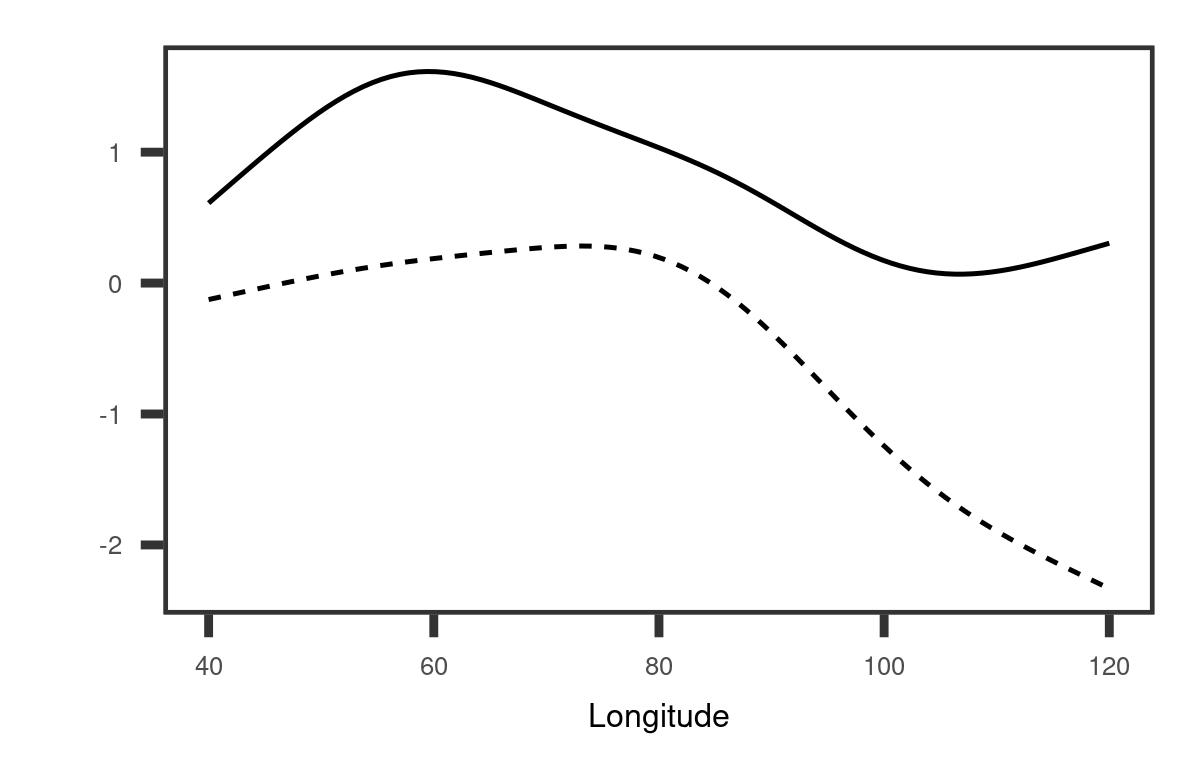
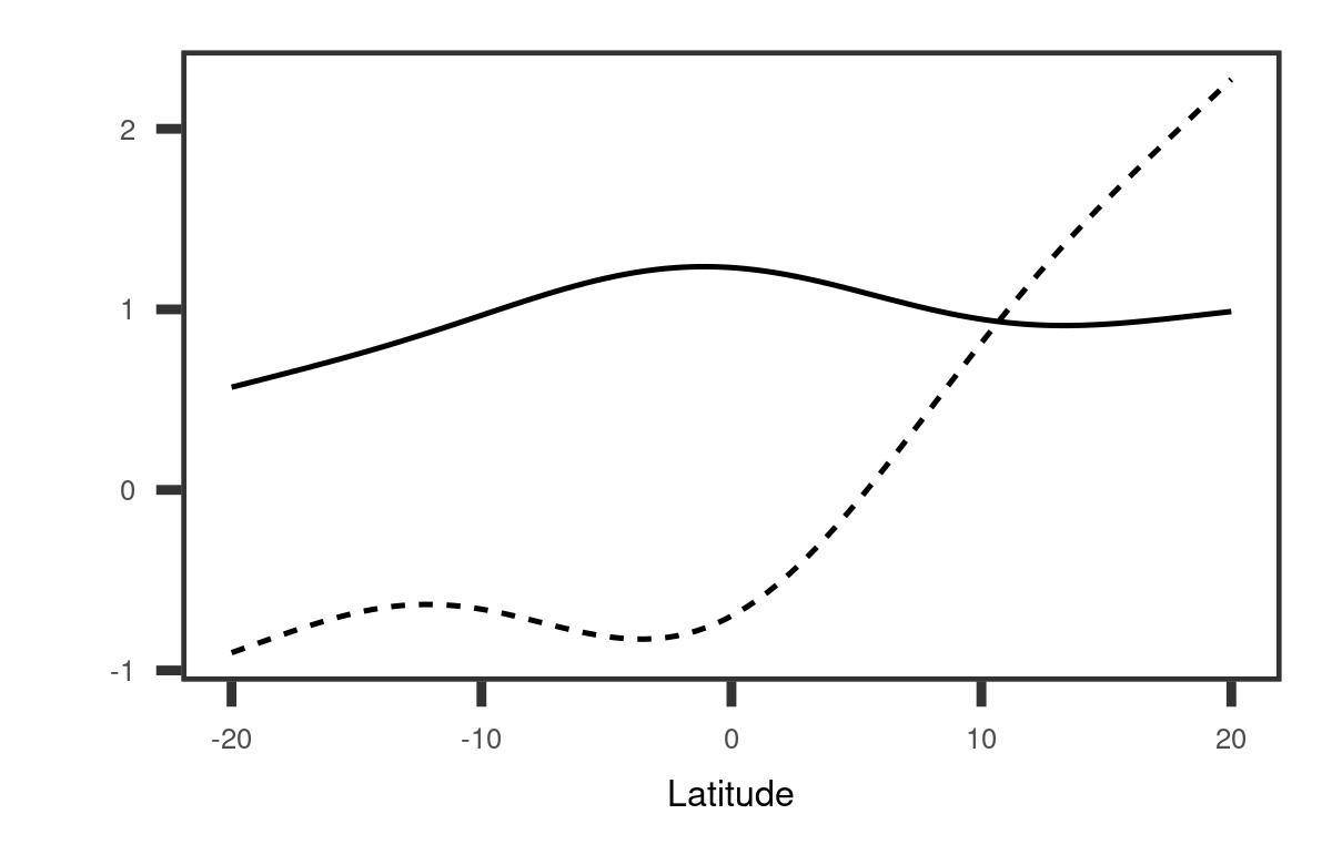
To provide a clearer understanding of the covariance function structure, we derived a marginal basis along longitude and latitude respectively. The details are given in Appendix A. The left panel of Figure 4 demonstrates that the first longitudinal marginal basis reflects a large variation in the western region while the second one corresponds to the variation in the eastern region. Due to different linear combinations, the variation along longitude may contribute to not only opposite changes between the eastern and western sides of the Indian Ocean as shown in the first two-dimensional eigenfunction, but also an overall warming or cooling tendency as shown in the second two-dimensional eigenfunction. The second longitudinal marginal basis reveals that the closer to the east boundary, the greater the variation is, which suggests that the IOD may be related to the Pacific Ocean. This aligns with the evidence that the IOD has a link with El Niño Southern Oscillation (ENSO) (Stuecker et al., 2017), an irregularly periodic variation in sea surface temperature over the tropical eastern Pacific Ocean. As shown in the right panel of Figure 4, the overall trend for the first latitude marginal basis is almost a constant function. This provides evidence that the IOD is primarily associated with the variation along longitude.
Appendix
Appendix A eigensystem and marginal basis
In this section, we present a transformation procedure to produce eigenfunctions and corresponding eigenvalues from our estimator obtained by (11).
Let , . Then , where and form a basis of , so . The eigenvalues of coincide with the eigenvalues of matrix , and the number of nonzero eigenvalues is the same as the rank of . The eigenfunction that corresponds to the -th eigenvalue of can be expressed as , where , are defined in Theorem 1, and with being the -th eigenvector of matrix . Using the property of Kronecker products, we have .
By simple verification, we can see that are one-dimensional orthonormal functions for dimension , . Therefore, we can also express with these one-dimensional basis and the coefficients will form a th order tensor of dimension . We use to represent this new coefficient tensor and extend our unfolding operators to space. It is easy to see that .
Since is a compact operator in the space, this yields a singular value decomposition which leads to a basis characterizing the marginal variation along the th dimension. We call it a marginal basis for the th dimension. Obviously the marginal basis function corresponding to the -th singular value for dimension can be expressed as , where , and is the -th singular vector of . And the marginal singular values of coincide with the singular values of matrix .
Appendix B Definitions of and
Here we provide the specific forms of and , which are closely related to the decay of . Specifically, is defined as the smallest positive such that
| (17) | |||
where is a universal constant, and is defined as the smallest positive such that
| (18) |
where is a constant depending on . The existences of and are shown in the proof of Theorem 2.
Supplementary Material
In the supplementary material related to this paper, we provide proofs of our theoretical findings and additional simulation results.
Acknowledgement
The research of Raymond K. W. Wong is partially supported by the U.S. National Science Foundation under grants DMS-1806063, DMS-1711952 (subcontract) and CCF-1934904. The research of Xiaoke Zhang is partially supported by the U.S. National Science Foundation under grant DMS-1832046. Portions of this research were conducted with high performance research computing resources provided by Texas A&M University (https://hprc.tamu.edu).
References
- Abernethy et al. (2009) Abernethy, J., F. Bach, T. Evgeniou, and J.-P. Vert (2009). A new approach to collaborative filtering: Operator estimation with spectral regularization. Journal of Machine Learning Research 10, 803–826.
- Allen (2013) Allen, G. I. (2013). Multi-way functional principal components analysis. In 2013 5th IEEE International Workshop on Computational Advances in Multi-Sensor Adaptive Processing (CAMSAP), pp. 220–223. IEEE.
- Bartlett et al. (2005) Bartlett, P. L., O. Bousquet, and S. Mendelson (2005). Local rademacher complexities. The Annals of Statistics 33(4), 1497–1537.
- Behera and Yamagata (2003) Behera, S. K. and T. Yamagata (2003). Influence of the indian ocean dipole on the southern oscillation. Journal of the Meteorological Society of Japan. Ser. II 81(1), 169–177.
- Boyd et al. (2010) Boyd, S., N. Parikh, E. Chu, B. Peleato, and J. Eckstein (2010). Distributed optimization and statistical learning via the alternating direction method of multipliers. Foundations and Trends® in Machine Learning 3(1), 1–122.
- Cai and Yuan (2010) Cai, T. T. and M. Yuan (2010). Nonparametric covariance function estimation for functional and longitudinal data. Technical report, Georgia Institute of Technology, Atlanta, GA.
- Cai and Yuan (2012) Cai, T. T. and M. Yuan (2012). Minimax and adaptive prediction for functional linear regression. Journal of the American Statistical Association 107(499), 1201–1216.
- Chen et al. (2017) Chen, K., P. Delicado, and H.-G. Müller (2017). Modelling function-valued stochastic processes, with applications to fertility dynamics. Journal of the Royal Statistical Society: Series B (Statistical Methodology) 79(1), 177–196.
- Chen and Müller (2012) Chen, K. and H.-G. Müller (2012). Modeling repeated functional observations. Journal of the American Statistical Association 107(500), 1599–1609.
- Chen and Jiang (2017) Chen, L.-H. and C.-R. Jiang (2017). Multi-dimensional functional principal component analysis. Statistics and Computing 27(5), 1181–1192.
- Chu et al. (2014) Chu, J.-E., K.-J. Ha, J.-Y. Lee, B. Wang, B.-H. Kim, and C. E. Chung (2014). Future change of the indian ocean basin-wide and dipole modes in the cmip5. Climate dynamics 43(1-2), 535–551.
- Deser et al. (2010) Deser, C., M. A. Alexander, S.-P. Xie, and A. S. Phillips (2010). Sea surface temperature variability: Patterns and mechanisms. Annual review of marine science 2, 115–143.
- Ferraty and Vieu (2006) Ferraty, F. and P. Vieu (2006). Nonparametric functional data analysis: theory and practice. Springer, New York.
- Goldsmith et al. (2011) Goldsmith, J., J. Bobb, C. M. Crainiceanu, B. Caffo, and D. Reich (2011). Penalized functional regression. Journal of Computational and Graphical Statistics 20(4), 830–851.
- Gu (2013) Gu, C. (2013). Smoothing Spline ANOVA Models (2nd ed.). New York: Springer.
- Hackbusch (2012) Hackbusch, W. (2012). Tensor spaces and numerical tensor calculus, Volume 42. Springer Science & Business Media.
- Halko et al. (2009) Halko, N., P.-G. Martinsson, and J. A. Tropp (2009). Finding structure with randomness: Stochastic algorithms for constructing approximate matrix decompositions. arXiv preprint arXiv:0909.4061.
- Hall and Vial (2006) Hall, P. and C. Vial (2006). Assessing the finite dimensionality of functional data. Journal of the Royal Statistical Society: Series B 68(4), 689–705.
- Horváth and Kokoszka (2012) Horváth, L. and P. Kokoszka (2012). Inference for functional data with applications, Volume 200. Springer, New York.
- Hsing and Eubank (2015) Hsing, T. and R. Eubank (2015). Theoretical foundations of functional data analysis, with an introduction to linear operators. John Wiley & Sons.
- Huang et al. (2009) Huang, J. Z., H. Shen, and A. Buja (2009). The analysis of two-way functional data using two-way regularized singular value decompositions. Journal of the American Statistical Association 104(488), 1609–1620.
- James et al. (2000) James, G. M., T. J. Hastie, and C. A. Sugar (2000). Principal component models for sparse functional data. Biometrika 87(3), 587–602.
- Kadkhodaie et al. (2015) Kadkhodaie, M., K. Christakopoulou, M. Sanjabi, and A. Banerjee (2015). Accelerated alternating direction method of multipliers. In Proceedings of the 21th ACM SIGKDD international conference on knowledge discovery and data mining, pp. 497–506. ACM.
- Kokoszka and Reimherr (2017) Kokoszka, P. and M. Reimherr (2017). Introduction to functional data analysis. CRC Press.
- Koltchinskii (2011) Koltchinskii, V. (2011). Oracle Inequalities in Empirical Risk Minimization and Sparse Recovery Problems: Ecole d’Eté de Probabilités de Saint-Flour XXXVIII-2008, Volume 2033. Springer Science & Business Media.
- Li and Song (2017) Li, B. and J. Song (2017). Nonlinear sufficient dimension reduction for functional data. The Annals of Statistics 45(3), 1059–1095.
- Li and Hsing (2010) Li, Y. and T. Hsing (2010). Uniform convergence rates for nonparametric regression and principal component analysis in functional/longitudinal data. The Annals of Statistics 38(6), 3321–3351.
- Liebl (2019) Liebl, D. (2019). Inference for sparse and dense functional data with covariate adjustments. Journal of Multivariate Analysis 170, 315–335.
- Lynch and Chen (2018) Lynch, B. and K. Chen (2018). A test of weak separability for multi-way functional data, with application to brain connectivity studies. Biometrika 105(4), 815–831.
- Mazumder et al. (2010) Mazumder, R., T. Hastie, and R. Tibshirani (2010). Spectral regularization algorithms for learning large incomplete matrices. Journal of machine learning research 11(Aug), 2287–2322.
- Mercer (1909) Mercer, J. (1909). Xvi. functions of positive and negative type, and their connection the theory of integral equations. Philosophical transactions of the royal society of London. Series A, containing papers of a mathematical or physical character 209(441-458), 415–446.
- Park and Staicu (2015) Park, S. Y. and A.-M. Staicu (2015). Longitudinal functional data analysis. Stat 4(1), 212–226.
- Paul and Peng (2009) Paul, D. and J. Peng (2009). Consistency of restricted maximum likelihood estimators of principal components. The Annals of Statistics 37(3), 1229–1271.
- Pearce and Wand (2006) Pearce, N. D. and M. P. Wand (2006). Penalized splines and reproducing kernel methods. The American Statistician 60(3), 233–240.
- Poskitt and Sengarapillai (2013) Poskitt, D. S. and A. Sengarapillai (2013). Description length and dimensionality reduction in functional data analysis. Computational Statistics & Data Analysis 58, 98–113.
- Ramsay and Silverman (2005) Ramsay, J. and B. Silverman (2005). Functional data analysis. Springer, New York.
- Raskutti et al. (2012) Raskutti, G., M. J. Wainwright, and B. Yu (2012). Minimax-optimal rates for sparse additive models over kernel classes via convex programming. The Journal of Machine Learning Research 13, 389–427.
- Reimherr et al. (2018) Reimherr, M., B. Sriperumbudur, and B. Taoufik (2018). Optimal prediction for additive function-on-function regression. Electronic Journal of Statistics 12(2), 4571–4601.
- Rice and Silverman (1991) Rice, J. A. and B. W. Silverman (1991). Estimating the mean and covariance structure nonparametrically when the data are curves. Journal of the Royal Statistical Society: Series B (Methodological) 53(1), 233–243.
- Shamshoian et al. (2019) Shamshoian, J., D. Senturk, S. Jeste, and D. Telesca (2019). Bayesian analysis of multidimensional functional data. arXiv preprint arXiv:1909.08763.
- Shinoda et al. (2004) Shinoda, T., H. H. Hendon, and M. A. Alexander (2004). Surface and subsurface dipole variability in the indian ocean and its relation with enso. Deep Sea Research Part I: Oceanographic Research Papers 51(5), 619–635.
- Stuecker et al. (2017) Stuecker, M. F., A. Timmermann, F.-F. Jin, Y. Chikamoto, W. Zhang, A. T. Wittenberg, E. Widiasih, and S. Zhao (2017). Revisiting enso/indian ocean dipole phase relationships. Geophysical Research Letters 44(5), 2481–2492.
- Sun et al. (2018) Sun, X., P. Du, X. Wang, and P. Ma (2018). Optimal penalized function-on-function regression under a reproducing kernel hilbert space framework. Journal of the American Statistical Association 113(524), 1601–1611.
- Tucker (1966) Tucker, L. R. (1966). Some mathematical notes on three-mode factor analysis. Psychometrika 31(3), 279–311.
- Ummenhofer et al. (2009) Ummenhofer, C. C., M. H. England, P. C. McIntosh, G. A. Meyers, M. J. Pook, J. S. Risbey, A. S. Gupta, and A. S. Taschetto (2009). What causes southeast australia’s worst droughts? Geophysical Research Letters 36(4).
- Wahba (1990) Wahba, G. (1990). Spline Models for Observational Data. Philadelphia: SIAM.
- Wang and Huang (2017) Wang, W.-T. and H.-C. Huang (2017). Regularized principal component analysis for spatial data. Journal of Computational and Graphical Statistics 26(1), 14–25.
- Wong et al. (2019) Wong, R. K. W., Y. Li, and Z. Zhu (2019). Partially linear functional additive models for multivariate functional data. Journal of the American Statistical Association 114(525), 406–418.
- Wong and Zhang (2019) Wong, R. K. W. and X. Zhang (2019). Nonparametric operator-regularized covariance function estimation for functional data. Computational Statistics & Data Analysis 131, 131–144.
- Xiao et al. (2013) Xiao, L., Y. Li, and D. Ruppert (2013). Fast bivariate p-splines: the sandwich smoother. Journal of the Royal Statistical Society: Series B (Statistical Methodology) 75(3), 577–599.
- Yao et al. (2005) Yao, F., H.-G. Müller, and J.-L. Wang (2005). Functional data analysis for sparse longitudinal data. Journal of the American Statistical Association 100(470), 577–590.
- Yuan and Cai (2010) Yuan, M. and T. T. Cai (2010). A reproducing kernel hilbert space approach to functional linear regression. The Annals of Statistics 38(6), 3412–3444.
- Zhang et al. (2013) Zhang, L., H. Shen, and J. Z. Huang (2013). Robust regularized singular value decomposition with application to mortality data. The Annals of Applied Statistics 7(3), 1540–1561.
- Zhang and Wang (2016) Zhang, X. and J.-L. Wang (2016). From sparse to dense functional data and beyond. The Annals of Statistics 44(5), 2281–2321.
- Zhou and Pan (2014) Zhou, L. and H. Pan (2014). Principal component analysis of two-dimensional functional data. Journal of Computational and Graphical Statistics 23(3), 779–801.
- Zhu et al. (2014) Zhu, H., F. Yao, and H. H. Zhang (2014). Structured functional additive regression in reproducing kernel hilbert spaces. Journal of the Royal Statistical Society: Series B 76(3), 581–603.
- Zipunnikov et al. (2011) Zipunnikov, V., B. Caffo, D. M. Yousem, C. Davatzikos, B. S. Schwartz, and C. Crainiceanu (2011). Multilevel functional principal component analysis for high-dimensional data. Journal of Computational and Graphical Statistics 20(4), 852–873.