Lower bounding the MaxCut of high girth 3-regular graphs using the QAOA
Abstract
We study MaxCut on 3-regular graphs of minimum girth for various ’s. We obtain new lower bounds on the maximum cut achievable in such graphs by analyzing the Quantum Approximate Optimization Algorithm (QAOA). For , at depth , the QAOA improves on previously known lower bounds. Our bounds are established through classical numerical analysis of the QAOA’s expected performance. This analysis does not produce the actual cuts but establishes their existence. When implemented on a quantum computer, the QAOA provides an efficient algorithm for finding such cuts, using a constant-depth quantum circuit. To our knowledge, this gives an exponential speedup over the best known classical algorithm guaranteed to achieve cuts of this size on graphs of this girth. We also apply the QAOA to the Maximum Independent Set problem on the same class of graphs.
1 Introduction
The MaxCut problem asks one to partition the vertices of a graph into two subsets to maximize the size of the “cut,” or the set of edges that cross between the subsets. Determining the maximum cut of a graph is NP-hard, one of Karp’s original 21 problems [1], and it remains NP-hard when restricted to 3-regular graphs [2]. Often one studies MaxCut as an approximate optimization problem, with the goal of finding a large cut.
Here we study MaxCut on 3-regular graphs with large girth. The girth of a graph is the length of its shortest cycle. We are interested in two questions: (1) How can we lower bound the maximum cut of a graph in terms of its girth, and (2) How can we use a classical or quantum algorithm to efficiently obtain a cut at least this large? We answer both questions through our analysis of the Quantum Approximate Optimization Algorithm (QAOA) [3]. While the first question is a mathematical question that does not concern algorithms, we prove a new lower bound constructively, by proving a performance guarantee on the QAOA applied to 3-regular graphs of sufficient girth. Here we have analyzed the performance of the QAOA without the need to actually run the algorithm. To find a cut of that size using the QAOA, you need to run the algorithm on quantum hardware. To our knowledge, the QAOA then provides an exponential speedup over the best known classical algorithms guaranteed to achieve a cut of this size, which require exponential time.
We quantify a cut by the cut fraction, that is, the fraction of edges that appear in the cut. For a graph , we can ask about the cut fraction of the largest cut, or for edge set . The smallest possible maximum cut fraction among all 3-regular graphs of girth at least is denoted
| (1) |
We use the infimum because the set of graphs with girth() is infinite, but (1) means that every graph of girth at least has a cut of size at least . The numerical value of is currently unknown for general .
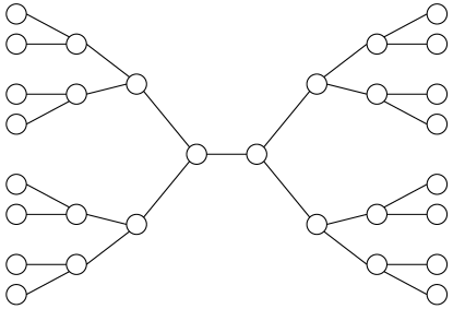
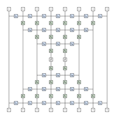
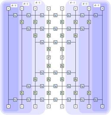
In this paper, we obtain new rigorous lower bounds on . We do this by predicting the performance of the QAOA for MaxCut on large girth 3-regular graphs. MaxCut may be viewed as an optimization problem over bit strings of length , where is the vertex set, and each bit string indicates a partition of the graph into two subsets. The QAOA is a quantum algorithm for approximate optimization over bit strings. It has a depth parameter and performance can only improve as increases. The QAOA produces a quantum state where the expectation of the MaxCut cost function is guaranteed to have a certain value. This means that there must exist cuts of at least this value. The MaxCut cost function is a sum of terms from each edge of the graph. For high-girth graphs, at each edge the neighborhood relevant to the QAOA is a tree. See Fig. 1 for an example at . To guarantee this we need . Each of these tree neighborhoods is isomorphic and at optimal parameters makes a contribution of for each edge of the graph. The total contribution to the quantum expected value of the cost, at optimal parameters, is . The size of the largest cut must be at least the size of the cut found by the QAOA. So we then have
| (2) |
for . So is lower bounded by a quantum expectation value.
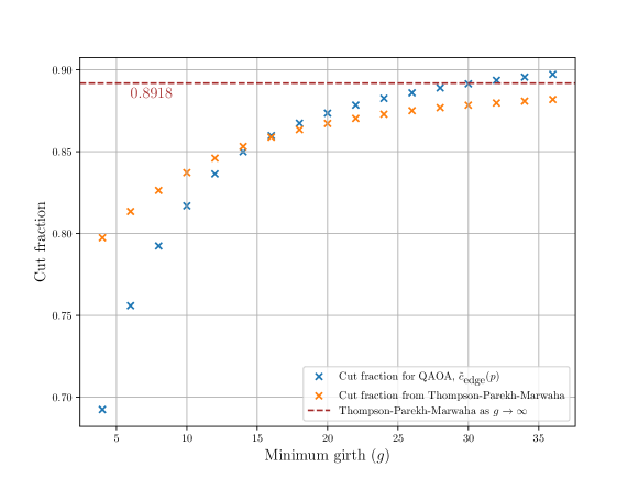
Our paper explains how we calculate with classical numerical computation. We get values for up to , corresponding to of . The numerical computations are highly accurate and the numbers we quote are good to at least four digits. In fact we have the best lower bound known to us for for any , improving on previous results by Thompson, Parekh, and Marwaha [4]. At and we are guaranteed a cut fraction of . See Fig. 2. Separately, from Refs. [5] and [6], one finds .
Actually running the QAOA on a graph has time-complexity , and it uses a constant-depth quantum circuit. For any 3-regular graph of girth , by using repeated applications of the QAOA, with total time-complexity , we can obtain a cut of size at least with probability . This may be viewed as an optimization or search problem with a promise (about the girth), with the goal of obtaining a cut of size above this threshold. There exist several classical algorithms for MaxCut, and we do not claim that the QAOA is superior in practice. However, besides the QAOA, we do not know any quantum or classical algorithms proven to solve this promise problem in subexponential time.
A natural point of comparison is the celebrated Goemans-Williamson (GW) algorithm [7]. The success of approximation algorithms is often measured by their approximation ratio: the ratio of the obtained value to the optimal value. The GW algorithm guarantees an approximation ratio of 0.878 for general graphs, and an improved ratio of 0.932 when specialized to graphs of maximum degree 3 [8]. Assuming the Unique Games Conjecture [9], it is NP-hard to exceed the GW algorithm’s 0.878 guarantee for the worst case. Our present analysis of the QAOA, however, focuses on cut fraction rather than approximation ratio. While our highest cut fraction guarantee of immediately guarantees an approximation ratio at least this size, such an approximation ratio is already exceeded by the specialized GW algorithm. Meanwhile, the GW algorithm does not provide any direct guarantee on cut fraction. So given a graph of girth , with the task of finding a cut of size at least , the GW algorithm is not guaranteed to succeed in general, while our specification of the QAOA provides an efficient algorithm. On the other hand, in the particular case of bipartite graphs (of any girth) the GW algorithm achieves the perfect cut, while the QAOA generally does not.
We briefly review QAOA, then describe the classical numerical methods used to obtain the performance guarantee. Our calculations are similar to the original calculations of Ref. [3], though performed at larger depth with distinct methods. We draw inspiration from the tensor network methods of Ref. [10], where the same QAOA quantities were calculated, though at lower depth . See also Refs. [11, 12] for related calculations at lower depth but including graphs of higher degree. Our main technical contribution is to analyze the QAOA for MaxCut on 3-regular graphs of large girth, using modified numerical methods to allow higher depth than previously obtained. We then interpret these results in relation to previous lower bounds for the maximum cut and previous algorithms for approximating its value. Finally we apply the QAOA to the problem of Maximum Independent Set on high-girth 3-regular graphs.
2 Review of the QAOA
The Quantum Approximate Optimization Algorithm (QAOA) is a quantum algorithm for finding approximate solutions to combinatorial optimization problems. We seek to optimize an objective function over bit strings, which is usually a sum over terms that each involves a few bits. The QAOA depends on an integer parameter and produces quantum states of the form
| (3) |
Here is the uniform superposition over computational basis states, is diagonal in the computational basis, and where is the sum of single-qubit Pauli X operators. The angles and are classical parameters which specify the QAOA state. For MaxCut, given a graph with vertices and edges , the cost function operator counts edges crossing between two subsets in a partition,
| (4) |
When measured in the computational basis, the state produces a bit string with a cost function value whose expectation is
| (5) |
The angles are optimized to maximize the expectation value . The quantum circuit depth grows with , and the performance at optimal parameters can only improve with larger .
3 Pre-computing QAOA parameters for graphs with large girth
Traditionally, the QAOA is executed by applying the quantum circuit with initial parameters, estimating through measurements, then using classical optimization to update and repeating the process. Here we take a different approach, emphasized especially by Ref. [10], where parameters are chosen in advance for all graphs of a given girth.
First note that the expectation value can be decomposed as a sum over edge terms. For MaxCut, each term depends only on the subgraph within distance of that edge. When a graph has girth at least
| (6) |
these neighborhoods are trees. Moreover, for all 3-regular graphs with this minimum girth, these trees are all isomorphic and make the same contribution to . We then can write
| (7) |
where
| (8) |
and can be any pair of neighboring nodes in since they all make identical contributions. Since (7) holds for all 3-regular graphs of girth at least , we have
| (9) |
for any . By finding optimal (or near optimal) parameters we improve the bound. We later discuss how we find the near optimal parameters . Let
| (10) |
Then we have
| (11) |
for any .
Wurtz and Lykov [10] computed up to and we reproduce these numbers. We compute up to . More precisely, for any fixed , we compute numerically using exact tensor network methods. The numerical error in the computation of is negligible compared to the 4-digit accuracy reported in our results. Then we maximize to obtain some approximately optimal parameters . Despite this approximate optimization, the value then serves as a precise lower bound for , due to (11).
When running the QAOA for graphs of girth greater than 36, it would be helpful to pre-compute the optimal parameters for , which we have not done. For sufficiently large this may be intractable, or it may be well-approximated by extrapolation of the optimal parameters from smaller to larger . Regardless, for the purpose of proposing a formal algorithm, for all 3-regular graphs of girth greater than 36, we propose running the QAOA with our fixed, pre-computed parameters. This protocol already gives an algorithm with polynomial runtime with respect to graph size, with the best currently known performance guarantee on cut fraction. The only other algorithms we currently know with the same performance guarantee take exponential time. One example is the the brute force algorithm, which finds the best cut in exponential time, and is therefore guaranteed to find a cut of size at least , whose existence follows from our present results. A classical algorithm of Williams [13] finds the best cut in exponential time but using a smaller exponent than brute force search.
4 Analyzing time-complexity
Here we detail the runtime of the QAOA as an algorithm running on a quantum computer to find an actual cut. (This analysis is separate from the classical numerical computations discussed in Section 5.2, which establish performance guarantees and serve as a pre-computation that is independent of problem instance.) We focus on the QAOA for -regular graphs on vertices, treating as a constant. The problem size is the number of edges, . The QAOA at depth uses total gates. When analyzing the runtime of quantum algorithms, we are interested in both the total number of gates and also the circuit depth, which counts the minimal number of layers such that each layer involves non-overlapping gates.
While the parameter is sometimes called the “depth” of the QAOA, its relation to circuit depth depends on the graph. The unitary can be implemented in a single layer of depth 1. On the other hand, while is naturally implemented by a two-qubit gate for every edge, these gates overlap whenever two edges share a vertex, so requires circuit depth larger than 1. Szegedy noted that one can use Vizing’s theorem to calculate the circuit depth [14]. For graph , the “edge chromatic number” is the minimal number of colors required for an edge-coloring where no two adjacent edges share the same color. By using a layer of gates for each color, we see can be implemented in depth using 2-local gates. Vizing’s theorem states that for general graphs, , where is the maximum degree. Again treating as a constant, we conclude has circuit depth, and the full QAOA has circuit depth . To achieve this -depth circuit, we need to classically pre-compute to actually find one of the colorings guaranteed by Vizing’s theorem. For a bounded degree graph, this computation runs in time [15], the same as the problem size, hence not contributing to the asymptotic complexity.
In this section, when we analyze the time complexity of running the QAOA on a quantum computer at fixed , we imagine running with fixed parameters given in advance. There is no outer loop variational search. The quantum circuit uses qubits, with gates and constant circuit depth.
After running the QAOA circuit and performing a measurement in the computational basis, we obtain a cut of the graph that depends on the measurement outcome. The expected value of the cut size is . We can also ask for a guarantee that the cut is above (the floor of) this expected value with high probability. To that end, repeat the QAOA circuit and measurement many times and record the best outcome. The probability of sampling a cut size of at least with a single sample is at least . So with repetitions, we obtain a sample with cut at least , with probability at least (or any constant probability below 1).
5 Numerical results and methods
5.1 Results
| 1 | 2 | 3 | 4 | 5 | 6 | 7 | 8 | 9 | |
|---|---|---|---|---|---|---|---|---|---|
| 10 | 11 | 12 | 13 | 14 | 15 | 16 | 17 | ||
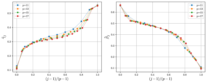
In order to maximize the quantum expected value of the cut size, we numerically evaluate the quantum expectation value of the cost function of Eq. (4). As we emphasized before, at the QAOA depths we consider, on these high girth graphs, each edge has an isomorphic tree neighborhood and so each edge gives the same contribution. We find values of that approximately maximize . For fixed the quantum expectation is evaluated using the tensor network contraction method described in Section 5.2. The blue crosses in Fig. 2 show the optimized values of at approximately optimal parameters, . The values are listed in Table 1. The parameters and are shown in Fig. 3 for different values of .
5.2 Methods
In order to evaluate , we consider the operator , as well as all quantum gates in the QAOA circuit contained in the light cone of this operator. In the simple case of , i.e., when is a line, the tensor network that evaluates is that of Fig. 5(a). Here we have followed the tensor definitions:
|
|
|
|||||
|
|
|
(12) |
where all tensor indices have support . Note that every gate of the form is diagonal, which we explicitly exploit in writing its corresponding tensor over only two variables and making use of hyperindices in the tensor network, corresponding to hyperedges in the underlying network.
In the generic case of the number of qubits in the light-cone of the operator grows exponentially with . For a 3-regular graph (i.e. ), at the size of the light cone is In general, for a -regular graph, the number of qubits at depth is . For and the size of the light-cone is 524,286 qubits. However, due to the fact that all branches in the regular tree are identical, we can perform this computation in a compact way that is not affected by the exponential growth in the number of qubits in the calculation. We contract a single branch inwards towards the root of the tree, raising its tensor entries to the th power before proceeding to the next level of the tree. This is expressed in graphical notation in Fig. 5(b), where we have made use of the definition
| (13) |
for the entrywise exponentiation of a tensor. Note that the cost of the evaluation of Eq. (8) as expressed in Fig. 5(b) has both time and space complexities that grow as . This is quadratically better than the time complexity reported in Refs. [11] and [12] for finite . Note also that the cost is independent of , in contrast to that of the method used in Ref. [10], which scales exponentially in and was run up to at and lower values of at larger . This allows us to evaluate and optimize Eq. (8) up to for any value of . Our implementation of the method is written in C++ and parallelized using OpenMP [18]. We also make use of the Eigen library for the manipulation of vectors [19] as well as the LBFGS++ library, which implements the Limited-memory BFGS algorithm for unconstrained optimization problems [20].
We remind the reader that all of our numerical methods are exact. We use computers to evaluate expressions, but there are no approximations. For and at depth we evaluate on a tree with vertices at a computational cost of . We go to p of 17. An alternate approach would be to use a quantum computer with qubits. Here we would evaluate the central edge of the tree using the full QAOA cost. Although we would be running a quantum computer, we would not be finding cuts but rather estimates of lower bounds on MaxCut values. It appears that this scales more favorably than our exact calculation of lower bounds, at least while . For this method to go beyond our result requires a highly accurate quantum computer capable of handling graphs with at least one million vertices. Repeated measurements would extract an accurate estimate of the quantum expectation but not a proof of a lower bound.
(a)
 (b)
(b)
6 MaxCut Comparisons
We can directly compare our results with those of Thompson, Parekh and Marwaha [4]. They have a classical algorithm for MaxCut which they apply to large girth graphs. They lower bound the performance of their algorithm to obtain lower bounds on for all . Using the formula found in Theorem 1 of their paper we can compare with our results. See Fig. 2. For any the QAOA (at appropriate ) finds cuts bigger than the TPM guarantees. Note that the limit as goes to infinity of their bound is which we exceed at of .
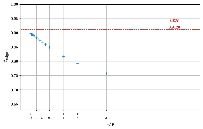
The results of Csóka et al [5] and Gamarnik and Li [6] imply that the limit as goes to infinity of is greater than or equal to 0.912. (These methods could in principle be used to find bounds on for finite , but as far as we know this has not been done.) Our numerical techniques are stretched to the limit at of and we do not have an analytic way of taking to infinity. See Fig. 4 where we plot versus and also show the target of 0.912. The reader can decide if we pass this target as increases, an empirical question left for future computations.
The graphs which we have considered have large girth and every edge sits in a tree neighborhood. We can ask about large random 3-regular graphs where almost all edges sit in tree neighborhoods. Such graphs have an order unity number of triangles, squares, pentagons, or any cycle of constant length, which means that they are not strictly large girth. However, since there are so few short cycles, any lower bound on for any is a lower bound on the cut fraction of a typical large random 3-regular graph [6]. Furthermore the QAOA at level achieves cut fraction on these graphs. There is an upper bound on the cut fraction of typical large random 3-regular graphs of 0.9351, described in Ref. [21] and shown by Hladky and McKay [16, 17]. Therefore the QAOA cut fraction cannot exceed 0.9351 even as . This value is shown in Fig. 4.
7 Maximum Independent Set
An independent set is a subset of the vertices of a graph with the property that there are no edges between any two members of the subset. The Maximum Independent Set problem (MIS) is to find the biggest independent set. The MIS problem is NP-hard for general graphs. Here we will use a general connection between independent sets and MaxCut that allows us to use our MaxCut results to get quick bounds on the independence ratio which is the fraction of vertices in the largest independent set. We then apply a variant of the QAOA to large-girth 3-regular graphs to establish better bounds on the independence ratio. We are not aware of any other bounds for MIS on this class of fixed girth graphs. However there are results in the limit as the girth goes to infinity [22].
| 1 | 2 | 3 | 4 | 5 | 6 | 7 | 8 | 9 | |
|---|---|---|---|---|---|---|---|---|---|
| Indep. ratio (2 params.) | 0.4051 | ||||||||
| Indep. ratio (3 params.) | 0.4094 | ||||||||
| 10 | 11 | 12 | 13 | 14 | 15 | 16 | 17 | ||
| Indep. ratio (2 params.) | 0.4228 | ||||||||
| Indep. ratio (3 params.) | 0.4244 |
A convenient local cost function for the MIS problem is
| (14) |
written as a function of the bit string , where each bit string also represents a subset of the vertex set , with if vertex is in the subset. Note this cost function is defined on all subsets and not just independent sets. The first term of is the Hamming weight which we want to make big, and the subtracted term counts violations of the independent set property. We now argue that given any bit string with associated cost , there exists an independent set of size at least . In particular, we consider the set of vertices labeled 1 in the bit string, and we construct a subset of these vertices that forms an independent set of size at least . To begin, given a bit string with cost , assume that the set of ’s is not yet an independent set. Choose any violated edge , that is with , then choose either or and re-label it as , that is, remove the vertex from the set under consideration. Consider the cost function for this new string: the bit flip decreases the Hamming weight by and decreases the number of violations by at least , so cannot decrease. Repeat this until there are no more violations so the final bit string must have ’s that form a valid independent set. The new value of is equal the size of the independent set which must be at least the original value of . Now the maximum of occurs when corresponds to an actual maximum independent set so achieving a high value of gives an approximation to the size of the largest independent set.
We now use the connection between MaxCut and independent sets to get a general bound on MIS. Consider the problem of maximizing the total number of vertices in two disjoint independent sets. We consider a cost function given by the sum of two terms, one for each set:
| (15) |
Write the two terms as . For any input bit string, the ’s represent one set and the ’s the complementary set. (Note that and here do not mean what they meant in the previous paragraph.) By the above argument regarding , first applied to , there exists a subset of ’s that forms an independent set, with size at least . Meanwhile, the same argument applied to implies there exists a subset of ’s that forms an independent set, with size at least . Thus we have two disjoint independent sets of total size at least .
We can rewrite Eq. (15) to get
| (16) |
where the sum on edges is the MaxCut cost. Let be the maximum fraction of combined vertices in two disjoint independent sets. Then for any graph,
| (17) |
where is the cut size associated to any bit string . For 3-regular graphs we get
| (18) |
As an aside, we note an interesting relation between and , where denotes the cut fraction of the best cut:
| (19) |
To see this, first note
| (20) |
which follows immediately from Eq. (18). This holds for any 3-regular graph with no restriction on girth. Now we refer to Gamarnik and Li [6]. From the argument in their Section 6, one can deduce
| (21) |
Together, these two inequalities yield the claimed Eq. (19) and we end our aside.
Let be the independence ratio, the fraction of vertices in the largest independent set. Then , since one of the two independent sets must contain at least half of their combined vertices. So from Eq. (18) we have
| (22) |
Taking the quantum expectation and using our MaxCut result for large girth 3-regular graphs we have
| (23) |
So we now have a lower bound on the independence ratio for any using the values from Table 1. These values are given as the first line in Table 2. In particular for girth at least we get a lower bound of .
But we can do better. Return to the cost function of Eq. (14). First we need to write it as a sum over edges. For 3-regular graphs,
| (24) |
Now using the fact that we can write the cost in terms of the operators which is more convenient,
| (25) |
Again we are looking at graphs with so each edge makes an identical contribution to the quantum expectation in the QAOA state. The quantum expectation equals the contribution from any edge times the number of edges , that is,
| (26) |
where as before is any edge in the graph, and is some state produced by the QAOA.
We are free to use any local operator to drive the QAOA. Here we modify the cost function part of the driver and but not the sum of the ’s. We will introduce two parameters, and , for each layer of the cost function unitary. In particular for the driving cost function operator we try
| (27) |
Including the at each layer there are a total of parameters. If , this amounts to using the MaxCut cost function as the driver. Using symmetry we can show that the linear term in the objective in expression (26) vanishes. So in fact with both the driver and objective function are those of MaxCut up to constants. Noting that and dividing (26) by gives, at optimal parameters, the right hand side of (23). If the ratio of to is set to the right constant, see expression (25), then the driver is the same as the objective function. So if we optimize over all ’s and ’s and ’s we do at least as well as using the MaxCut cost function as the driver or the local MIS cost function as the driver. In Table 2 we give lower bounds on the independence ratio for MIS produced by this optimization over parameters.
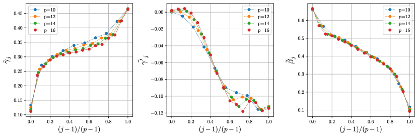
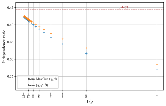
In Fig. 6 we show the lower bounds we get on the independence ratio as a function of from our MaxCut results and using the -parameter per layer ansatz. The -parameter ansatz must lie above the other but the difference shrinks as grows. The red line is the best available bound on the independence ratio for large girth 3-regular graphs as the girth goes to infinity [22]. The optimized parameters are shown in Fig. 7 for different values of .
To find independent sets which meet these guarantees you can run the QAOA on quantum hardware with constant circuit depth for a constant . This gives a polynomial-time quantum algorithm for this problem. We know of no classical algorithm that performs as well (in terms of guaranteed independence ratio) on the problem of MIS on 3-regular graphs of girth at least .
8 Conclusions
We proved a new lower bound for MaxCut on high-girth graphs by using a classical computer to analyze the performance of a quantum algorithm. This graph-theoretic result holds even if quantum computing is infeasible. We are unaware of other examples where the analysis of quantum algorithmic performance yields similarly novel results.
Running the quantum algorithm on a quantum computer would efficiently find the actual cuts that achieve our lower bounds. This provides an exponential speedup for finding these cuts, compared to known classical algorithms with rigorous guarantees.
9 Acknowledgements
This project was an outgrowth of a project which included Brandon Augustino, Madelyn Cain, Swati Gupta, Eugene Tang and Katherine Van Kirk. We are grateful to them for getting us going. We also thank Ojas Parekh and Kunal Marwaha for reading our manuscript. We thank David Gamarnik for suggesting that we look at MIS. We thank Joao Basso, Stephen Jordan and Mario Szegedy for helpful comments and Leo Zhou for introducing the idea of the last paragraph of Section 5.2. DR acknowledges support by the Simons Foundation under grant 376205.
References
- [1] Richard M Karp. On the computational complexity of combinatorial problems. Networks, 5(1):45–68, 1975.
- [2] Mihalis Yannakakis. Node-and edge-deletion np-complete problems. In Proceedings of the tenth annual ACM symposium on Theory of computing, pages 253–264, 1978.
- [3] Edward Farhi, Jeffrey Goldstone, and Sam Gutmann. A quantum approximate optimization algorithm. arXiv preprint arXiv:1411.4028, 2014.
- [4] Jessica K Thompson, Ojas Parekh, and Kunal Marwaha. An explicit vector algorithm for high-girth maxcut. In Symposium on Simplicity in Algorithms (SOSA), pages 238–246. SIAM, 2022.
- [5] Endre Csóka, Balázs Gerencsér, Viktor Harangi, and Bálint Virág. Invariant gaussian processes and independent sets on regular graphs of large girth. Random Structures & Algorithms, 47(2):284–303, 2015.
- [6] David Gamarnik and Quan Li. On the max-cut of sparse random graphs. Random Structures & Algorithms, 52(2):219–262, 2018.
- [7] Michel X Goemans and David P Williamson. Improved approximation algorithms for maximum cut and satisfiability problems using semidefinite programming. Journal of the ACM (JACM), 42(6):1115–1145, 1995.
- [8] Eran Halperin, Dror Livnat, and Uri Zwick. Max cut in cubic graphs. Journal of Algorithms, 53(2):169–185, 2004.
- [9] Subhash Khot. On the power of unique 2-prover 1-round games. In Proceedings of the thiry-fourth annual ACM symposium on Theory of computing, pages 767–775, 2002.
- [10] Jonathan Wurtz and Danylo Lykov. The fixed angle conjecture for qaoa on regular maxcut graphs. arXiv preprint arXiv:2107.00677, 2021.
- [11] Joao Basso, Edward Farhi, Kunal Marwaha, Benjamin Villalonga, and Leo Zhou. The quantum approximate optimization algorithm at high depth for maxcut on large-girth regular graphs and the sherrington-kirkpatrick model. arXiv preprint arXiv:2110.14206, 2021.
- [12] Elisabeth Wybo and Martin Leib. Missing puzzle pieces in the performance landscape of the quantum approximate optimization algorithm. arXiv preprint arXiv:2406.14618, 2024.
- [13] Ryan Williams. A new algorithm for optimal 2-constraint satisfaction and its implications. Theoretical Computer Science, 348(2-3):357–365, 2005.
- [14] Mario Szegedy. What do qaoa energies reveal about graphs? arXiv preprint arXiv:1912.12277, 2019.
- [15] Anton Bernshteyn and Abhishek Dhawan. Fast algorithms for vizing’s theorem on bounded degree graphs. arXiv preprint arXiv:2303.05408, 2023.
- [16] Jan Hladkỳ. Structural properties of graphs—probabilistic and deterministic point of view. 2006.
- [17] Brendan D McKay. Maximum bipartite subgraphs of regular graphs with large girth. In Proc. 13th SE Conf. on Combin. Graph Theory and Computing, Boca Raton, Florida, volume 436, 1982.
- [18] Leonardo Dagum and Ramesh Menon. OpenMP: an industry standard API for shared-memory programming. Computational Science & Engineering, IEEE, 5(1):46–55, 1998.
- [19] Gaël Guennebaud, Benoît Jacob, et al. Eigen v3. Online, 2010.
- [20] Yixuan Qiu and Dirk Toewe. LBFGS++. Online, 2020.
- [21] František Kardoš, Daniel Král, and Jan Volec. Maximum edge-cuts in cubic graphs with large girth and in random cubic graphs. Random Structures & Algorithms, 41(4):506–520, 2012.
- [22] Endre Csóka. Independent sets and cuts in large-girth regular graphs. arXiv preprint arXiv:1602.02747, 2016.