LPHE-MS-Sept-24-revised
Topological 4D gravity and
gravitational defects

Y. Boujakhrout ¹¹1boujakhroutyoussra@gmail.com, R. Sammani, E.H Saidi
1. LPHE-MS, Science Faculty, Mohammed V University in Rabat, Morocco
2. Centre of Physics and Mathematics, CPM- Morocco

Abstract

Using the Chern-Simons formulation of AdS₃ gravity as well as the Costello-Witten-Yamazaki (CWY) theory for quantum integrability, we construct a novel topological 4D gravity given by Eq(5.1) with observables based on gravitational gauge field holonomies. The field action $\mathcal{S}_{4D}^{grav}$ of this gravity has a gauge symmetry $SL(2,\mathbb{C})$ and reads also as the difference $\mathcal{S}_{4D}^{CWY_{L}}-\mathcal{S}_{4D}^{CWY_{R}}$ with 4D Chern-Simons field actions $\mathcal{S}_{4D}^{CWY_{L/R}}$ given by left/right CWY theory Eq(3.9). We also use this 4D gravity derivation to build observables describing gravitational topological defects and their interactions. We conclude our study with few comments regarding quantum integrability and the extension of AdS₃/CFT₂ correspondence with regard to the obtained topological 4D gravity.

Keywords: AdS₃ gravity and CS formulation, AdS₃/CFT₂, Line defects in CS and 4D gravity, Integrable spin chains and brane realisations in strings.

1 Introduction

Following [1], the 3D Chern-Simons theory with hermitian gauge field action $\mathcal{S}_{3D}^{{\small CS}}\left[A\right]$ has an unconventional 4D extension giving a powerful QFT framework to study quantum integrability [2]-[4]. This is an exotic 4D extension of the usual 3D Chern-Simons (CS) modeling to which we refer below to as the Costello-Witten-Yamazaki theory. It lives in a 4D space $\boldsymbol{M}_{4D}$ fibered like $\Sigma_{2}\times\tilde{\Sigma}_{2}$ ; that is the products of two 2D real surfaces thought of in this study as $\mathbb{R}^{2}\times\mathbb{CP}^{1}$ with complex projective line isomorphic to the real 2-sphere $\mathbb{S}^{2}$ [5]. The Costello-Witten-Yamazaki (CWY) theory is a 4D topological quantum field theory with field action $\mathcal{S}_{4D}^{{\small CWY}}\left[\mathbf{A}\right]$ leading to a flat 2-form gauge curvature F ${}_{2}=d\mathbf{A}+\mathbf{A}^{2}=0$ . Its observables are given by line and surface defects that have been shown to carry precious information on quantum integrability [6]-[13]. Typical gauge invariant line defects are given by Wilson and ’t Hooft lines as well as their braiding [14],[15]. These line defects have been given interpretations in terms of Q-operators of integrable quantum spin and superspin chains [16]; and were realised in terms of intersecting branes in type II strings and M-theory [17]-[19]. The main steps in the derivation of the CWY theory by starting from the 3D Chern-Simons are given in section 3; we refer to these steps as the Building ALgorithm (BAL); this BAL will be in our construction.

On the other hand, it is quite well known that 3D Anti-de Sitter (AdS₃) gravity is intimately related with 3D Chern-Simons theory [20]-[24]. The field action $\mathcal{S}_{AdS_{3}}^{grav}\left[\mathbf{e,\omega}\right]$ of the AdS₃ gravity is a functional of two 1-forms given by the real dreibein $\mathbf{e}$ and the real 3D spin connection $\mathbf{\omega}$ . But it has been shown that $\mathbf{e}$ and $\ \mathbf{\omega}$ can be expressed in terms of left/right pair ( $A_{L},A_{R}$ ) of Chern-Simons gauge fields in 3D. In this CS description, the $\mathbf{\omega}$ is given by the mean field ( $A_{L}+A_{R}$ )/2 and $\mathbf{e}$ by the reduced field variable ( $A_{L}-A_{R}$ )/2. Concretely, it was found that the $\mathcal{S}_{AdS_{3}}^{grav}$ can be nicely formulated like the difference of two Chern-Simons field actions as

\mathcal{S}_{AdS_{3}}^{grav}=\mathcal{S}_{3D}^{{\small CS}}\left[A_{L}\right]-\mathcal{S}_{3D}^{{\small CS}}\left[A_{R}\right]

(1.1)

where $A_{L}$ and $A_{R}$ are hermitian 1-form CS gauge potentials valued in left and right Lie algebras; say $A_{L}$ valued in $sl(2,\mathbb{R})_{L}$ and $A_{R}$ valued in $sl(2,\mathbb{R})_{R}.$ Because of its rich properties, the AdS₃ gravity has been the subject of increasing interest; especially in connection with AdS₃/CFT₂ correspondence [22, 23, 25], BTZ black holes [26] and higher spin 3D gravities [22, 23, 27].

In this paper, we contribute to the study of AdS₃ gravity from the view of quantum integrability and topological gravitational defects. For that, we apply the method of CWY of integrable systems to the AdS₃ gravity with Anti-de Sitter group $SO(2,2)$ while using its formulation in terms of the CS gauge potentials $A_{L/R}$ . In this way, one opens a window on applications of integrable system methods obtained by CWY in QFT to 4D topological gravity with line and surface defects. The outcome of this study is twofold:

First, the derivation of a novel 4D topological gravity living on the 4D space $\mathbb{R}^{2}\times\mathbb{CP}^{1}$ with field action $\mathcal{S}_{4D}^{grav}$ that can be expressed in two equivalent ways: $\left(\mathbf{i}\right)$ as a functional of a 4D left $\mathbf{A}_{L}$ and a 4D right $\mathbf{A}_{R}$ Chern-Simons like fields (two CWY gauge fields $\mathbf{A}_{L}/\mathbf{A}_{R}$ ) as follows

\mathcal{S}_{4D}^{grav}\left[\mathbf{A}_{L}\mathbf{,A}_{R}\right]=\mathcal{S}_{4D}^{{\small CWY}}\left[\mathbf{A}_{L}\right]-\mathcal{S}_{4D}^{{\small CWY}}\left[\mathbf{A}_{R}\right]

(1.2)

with $\mathcal{S}_{4D}^{{\small CWY}}\left[\mathbf{A}_{L/R}\right]$ given by eqs(4.2-4.8); or $\left(\mathbf{ii}\right)$ like the functional $\mathcal{S}_{4D}^{grav}\left[\mathbf{E,\Omega}\right]$ reading as in eq(5.1). The four dimensional $\mathbf{E}$ and $\mathbf{\Omega}$ are the vielbein and the spin connection 1-forms living on $\mathbb{R}^{2}\times\mathbb{CP}^{1}$ and valued in $sl(2,\mathbb{C})$ . These gravity potentials are given by linear combinations $(\mathbf{A}_{L}\pm\mathbf{A}_{R})/2$ in a similar fashion to the Achucarro-Townsend 3D Chern- Simons derivation. We show that the two point correlation functions $\left\langle\mathbf{E}(\zeta_{1})\mathbf{E}(\zeta_{2})\right\rangle$ and $\left\langle\mathbf{\Omega}(\zeta_{1})\mathbf{\Omega}(\zeta_{2})\right\rangle$ vanish identically while $\left\langle\mathbf{E}(\zeta_{1})\mathbf{\Omega}(\zeta_{2})\right\rangle$ is a non vanishing propagator $\boldsymbol{P}(\zeta_{1}-\zeta_{2})$ given by eqs(4.33-4.35).

Second, considering the above 4D topological field action (1.2) with $\mathbf{E}$ and $\mathbf{\Omega}$ expressed in terms of CYW connections $(\mathbf{A}_{L}\pm\mathbf{A}_{R})/2$ , we obtain two types of 4D gravitational line defects W ${}_{E}\left[\mathrm{\gamma}_{z}\right]$ and W ${}_{\Omega}\left[\mathrm{\gamma}_{w}\right]$ described by topological observables based on the holonomy of the topological gravitational 1-form potentials

\Phi_{E}=\mathop{\displaystyle\oint}\nolimits_{\mathrm{\gamma}_{z}}\mathbf{E}\qquad,\qquad\Phi_{\Omega}=\mathop{\displaystyle\oint}\nolimits_{\mathrm{\gamma}_{w}}\mathbf{\Omega}

(1.3)

with loops $\mathrm{\gamma}_{z}$ and $\mathrm{\gamma}_{w}$ spreading in the topological plane $\mathbb{R}^{2}$ and located at the points z and w in $\mathbb{CP}^{1}\simeq\mathbb{S}^{2}$ . Moreover, using the topological invariant $\mathcal{S}_{4D}^{grav}$ as well as the vielbein and spin connection line defects, we give partial results on quantum integrability including Yang-Baxter and RLL equations; and comment on the extension of the AdS₃/CFT₂ correspondence in the new framework of 4D topological gravity (1.2).

Before proceeding, we would like to emphasise that the derivation of the field action (1.2) of the 4D topological gravity will be carried out in three consecutive steps 1, 2 and 3 as indicated by the following diagram in Table 1.

3D : AdS₃ gravity $S_{AdS_{3}}^{grav}\left[e,\omega\right]$ $\ \ \ \underrightarrow{\text{ \ \ step }1\text{ \ \ }}$ $S_{3D}^{cs}\left[A_{L}\right]-S_{3D}^{cs}\left[A_{R}\right]$ $\downarrow$ $\ \ \text{steps }1$ - $2$ - $3$ $\downarrow$ step $2$ 4D : 4D gravity $S_{4D}^{grav}\left[E,\Omega\right]$ $\underleftarrow{\text{ \ \ step }3\text{ \ \ \ }}$ $S_{4D}^{cyw}\left[A_{L}\right]-S_{4D}^{cyw}\left[A_{R}\right]$

Table 1: the way diagram to build 4D topological gravity by starting from AdS₃ gravity. The way is achieved into three steps 1, 2 and 3 as indicated by the arrows.

The organisation of the paper is as follows: In section 2, we revisit useful aspects of the Chern-Simons formulation of AdS₃ gravity and its boundary CFT₂. In section 3, we give the building algorithm (BAL) for the derivation of the CWY theory by starting from the usual 3D-Chern-Simons. In section 4, we develop the basis of the 4D topological gravity deduced from the AdS₃ gravity and investigate the topological defects within. Section 5 is devoted to conclusion and comments with regards to integrable quantum spin chains and the extension of AdS₃/CFT₂ correspondence.

2 Chern-Simons formulation of AdS₃ gravity

We begin by describing the Anti-de Sitter 3D gravity with spacetime metric $g_{\mu\nu}=e_{\mu}^{a}\eta_{ab}e_{\nu}^{b}$ where $\eta_{ab}$ is the usual flat $diag(-,+,+)$ of 3D with rotation group in tangent space given by $SO\left(1,2\right).$ This non compact space is a maximally symmetric solution of 3D Einstein’s equation with a negative cosmological constant (negative constant curvature). By using the Dreibein $e_{\mu}^{a}$ and the (dualized) spin connection $\omega_{\mu}^{a}$ of AdS₃ as well as the associated 1-forms $e^{a}=e_{\mu}^{a}dx^{\mu}$ and $\omega^{a}=\omega_{\mu}^{a}dx^{\mu}$ invariant under Diff(AdS₃) but transforming as $SO\left(1,2\right)$ vectors, the field action $\mathcal{S}_{{\small 3D}}^{{\small grav}}=\mathcal{S}_{{\small 3D}}^{{\small grav}}\left[e,\omega\right]$ of the AdS₃ gravity reads in differential form language as follows [20, 22, 29, 30]

\mathcal{S}_{{\small 3D}}^{{\small grav}}=\frac{1}{8\pi G}\mathop{\displaystyle\int}\nolimits_{\mathcal{M}_{3D}}\mathcal{L}_{3}^{grav}

(2.1)

The 3-form Lagrangian density reads in terms of the curvature 2-form $\mathcal{R}_{a}$ like,

$\mathcal{L}_{3}^{grav}$	$=$	$e^{a}\wedge\mathcal{R}_{a}+\frac{\xi}{3!}\varepsilon_{abc}e^{a}\wedge e^{b}\wedge e^{c}$
$\mathcal{R}_{a}$	$=$	$d\omega_{a}+\frac{1}{2}\varepsilon_{abc}\omega^{b}\wedge\omega^{c}$

(2.2)

where for convenience we have set $\xi=8\pi G_{N}/l_{{\small AdS}}^{2}$ with $l_{{\small AdS}}$ the AdS₃ radius and $G_{N}$ the Newton constant in 3D. The field equations of motion following from the above $\mathcal{S}_{{\small 3D}}^{{\small grav}}$ are given by

$\mathcal{R}_{a}$	$=$	$-\frac{\xi}{2}\varepsilon_{abc}e^{b}\wedge e^{c}$
$de_{a}$	$=$	$-\frac{1}{2}\varepsilon_{abc}e^{b}\wedge\omega^{c}$

(2.3)

and are solved by the AdS₃ metric [31]. Notice that the 3D field action $\mathcal{S}_{{\small 3D}}^{{\small grav}}$ is sometimes termed as the spin $s_{cft}=2$ AdS₃ gravity; a terminology due to the AdS₃/CFT₂ correspondence [22, 25, 32]. This duality means that on the boundary of AdS₃ lives a scale invariant field theory with quantum states described by conformal symmetry generated by a conformal spin $s_{cft}=2$ current T_zz satisfying the Virasoro algebra [28].

On the other hand, following [20, 22, 23, 28], the gravity field action $\mathcal{S}_{{\small 3D}}^{{\small grav}}$ given by (2.2) can be expressed like the difference of two Chern-Simons field actions as follows

\mathcal{S}_{{\small 3D}}^{{\small grav}}=\mathcal{S}_{{\small 3D}}^{{\small CS}}\left[A_{L}\right]-\mathcal{S}_{{\small 3D}}^{{\small CS}}\left[A_{R}\right]

(2.4)

with

\mathcal{S}_{{\small 3D}}^{{\small CS}}\left[A\right]=\frac{k}{4\pi}\mathop{\displaystyle\int}\nolimits_{\mathcal{M}_{3D}}Tr\left(AdA+\frac{2}{3}A^{3}\right)

(2.5)

In the eqs(2.5), the Chern-Simons levels $k_{L}$ and $k_{R}$ are taken equal; and the $A_{L}=A_{L}(x^{0},x^{1},x^{2})$ and $A_{R}=A_{R}(x^{0},x^{1},x^{2})$ are the 3D Chern-Simons gauge potentials. They are valued in the $SO\left(1,2\right)_{L}$ and $SO\left(1,2\right)_{R}$ gauge symmetries having the homomorphisms

SO\left(1,2\right)\simeq SU\left(1,1\right)\simeq SL\left(2,\mathbb{R}\right)

(2.6)

These Chern-Simons 1-forms $A_{L}$ and $A_{R}$ expand in terms of the space-time 1-forms $dx^{\mu}$ and the three $SU\left(1,1\right)$ generators $J_{a}$ like

A=A^{a}J_{a}=dx^{\mu}A_{\mu}=dx^{\mu}A_{\mu}^{a}J_{a}

(2.7)

The link between the CS gauge fields $A_{L},$ $A_{R}$ and the gravity fields $e_{\mu}^{a},$ $\omega_{\mu}^{a}$ is given by the Achucarro-Townsend relations [20, 22, 23]

$A_{L}^{a}$	$=$	$\omega^{a}+\frac{1}{l_{{\small AdS}}}e^{a}$
$A_{R}^{a}$	$=$	$\omega^{a}-\frac{1}{l_{{\small AdS}}}e^{a}$

(2.8)

In what follows, we set $l_{{\small AdS}}=1$ for simplicity; and by using eq(2.7), we then have $A_{L/R}^{a}=\omega^{a}\pm e^{a}$ . With the relations (2.1-2.2) and (2.4-2.5) as well as (2.8), we have completed the step-1 in the way diagram of Table 1.

3 From 3D Chern-Simons to CWY theory

First, we recall useful aspects of the 3D Chern-Simons theory; then we give the Building ALgorithm (BAL) where we briefly describe the main pillars to extend the 3D Chern-Simons theory to the CWY theory. This investigation constitutes the second step of Table 1 towards the derivation of the novel topological 4D gravity (1.2).

3.1 More on 3D Chern-Simons action

In 3D, the Chern-Simons gauge field action $\mathcal{S}_{3D}^{{\small CS}}=\int_{\mathcal{M}_{3D}}\mathcal{L}_{3}^{{\small CS}}$ with generic gauge symmetry G depends on the 1-form gauge potential field $dx^{\mu}A_{\mu}^{a}$ as follows [33]

\mathcal{L}_{3}^{{\small CS}}=A^{a}\wedge dA_{a}+\frac{2}{3}\varepsilon_{abc}A^{a}\wedge A^{b}\wedge A^{c}

(3.1)

Here, we will think about G either as $SU\left(2\right)$ or like $SU\left(1,1\right)$ having the homomorphisms (2.6). These two gauge symmetries are the two real forms of the complex $SL(2,\mathbb{C})$ which turns out to play a basic role in our derivation of 4D topological gravity. In passing, note that when considering applications in 3D higher spin theory, the tangent space of the 3D spacetime can be imagined either as the euclidian $\mathbb{R}^{3}$ with $SO\left(3\right)\simeq SU\left(2\right)$ isotropy, or like the Lorentzian $\mathbb{R}^{1,2}$ with $SO\left(1,2\right)\simeq SU\left(1,1\right)$ symmetry.

The field equation of the three dimensional $SL\left(2,\mathbb{R}\right)$ CS gauge field is given by

F_{a}=dA_{a}+\varepsilon_{abc}A^{b}\wedge A^{c}=0

(3.2)

By using the expansions $A\left(x\right)=A^{a}\left(x\right)J_{a}$ and $F\left(x\right)=F^{a}\left(x\right)J_{a}$ in terms of the generators $J_{a}$ of the Lie algebra of the gauge symmetry, the above field equation reads shortly as follows

F=dA+A\wedge A=0

(3.3)

So, the CS gauge field $A$ has a flat curvature showing that the 3D Chern-Simons theory has no observable constructed out of the 2-form $F.$ However, one can still build gauge invariant observables in this topological 3D gauge theory; they are given by gauge topological line defects such as the Wilson loops $\mathrm{\gamma}$ on which propagate quantum states $\left|\lambda\right\rangle$ sitting in some representation $\boldsymbol{R}$ of the gauge symmetry G. These observables are built as [1],

W_{\boldsymbol{R}}\left[\mathrm{\gamma}\right]=Tr_{\boldsymbol{R}}\left[P\exp\left(\mathop{\displaystyle\oint}\nolimits_{\mathrm{\gamma}}A\right)\right]

(3.4)

where for the case $G=SU\left(2\right)$ , the $\boldsymbol{R}$ representation (labeled as $\boldsymbol{R}_{j}$ ) have spin states $\left|j,m\right\rangle$ sitting in multiplets $\mathfrak{M}_{j}$ with dimension $2j+1.$ This construction extends straightforwardly to the classical gauge symmetries in the Cartan classification of Lie algebras; but here below we will focuss on the real forms of $SL\left(2,\mathbb{C}\right)$ .

3.2 CWY theory: building algorithm

The CWY theory is a 4D topological quantum field theory that can derived from the usual 3D Chern-Simons theory using BAL[1]. This topological QFT_4D also has a six dimensional origin [34]. From a practical point of view, the CWY construction is a complexified gauge theory living on the 4D space $\boldsymbol{M}_{4}=\Sigma_{2}\times C$ with $\Sigma_{2}$ a real surface thought of here as $\mathbb{R}^{2}$ ; and $C$ a complex curve which can be either $\left(i\right)$ the complex projective line $\mathbb{CP}^{1}$ , $\left(ii\right)$ the complex line $\mathbb{C}^{\times}$ without the origin; or $\left(iii\right)$ an elliptic curve $\mathcal{E}$ . This theory has been a subject of big interest in the few last years especially when it comes to quantum integrability and brane realisation of integrable systems [17, 18, 19, 35].

Below, we give a rough re-derivation of this theory; starting from eq(3.1) and following [1], one can construct a 4D extension of the usual 3D Chern-Simons gauge theory by performing some surgery on the 3D Chern-Simons theory. The building algorithm of the 4D topological CWY theory from 3D-Chern-Simons may be done into three steps as follows.

$\left(\mathbf{1}\right)$

the 3D space $\mathcal{M}_{3D}$ in the CS field action

\mathcal{S}_{3D}^{{\small CS}}=\int_{\mathcal{M}_{3D}}\mathcal{L}_{3}^{{\small CS}}

(3.5)

is broken to $R_{t}\times\Sigma_{2}$ . The surface $\Sigma_{2}$ is named the real topological plane where spread the gauge invariant line defects $\mathrm{\gamma}$ of the CWY theory. The real line $\mathrm{\gamma}$ can be imagined in terms of sites in the integrable quantum spin chain; or as branes intersection line in type II strings and M- theory [17]-[19]. In what follows, this surface $\Sigma_{2}$ will be taken as $\mathbb{R}^{2}$ .

$\mathbf{(2)}$

promote the time axis $R_{t}$ to a complex line $C$ with local coordinate $z=x^{3}+it$ ; this is possible by adding a fourth coordinate $x^{3}$ to the old three ( $t,x^{1},x^{2}$ ); thus leading to ( $t,x^{1},x^{2},x^{3}$ ) imagined as ( $x,y,z,\bar{z}$ ). Here, we think about this $z$ as the local coordinate of the projective $\mathbb{CP}^{1}$ which is isomorphic to the real 2-sphere $\mathbb{S}^{2}.$ The complex line $C$ in the CWY theory is sometimes termed as the holomorphic plane. With this surgery, the space $\mathcal{M}_{3D}$ of the Chern-Simons theory becomes a 4D space $\boldsymbol{M}_{4}$ factorised like

\boldsymbol{M}_{4}=\Sigma_{2}\times\mathbb{CP}^{1}=\mathbb{R}^{2}\times\mathbb{S}^{2}

(3.6)

Regarding the fields and symmetries of the CWY theory, we have the following emerging quantities: $\left(i\right)$ Under surgery, the initial 1-form 3D CS gauge field $A^{a}\left(x,y,t\right)$ with expansion $A^{a}=A_{x}^{a}dx+A_{y}^{a}dy+A_{t}^{a}dt$ becomes a complex 4D gauge field $\boldsymbol{A}^{a}=\boldsymbol{A}^{a}\left(x,y,z,\bar{z}\right)$ with the expansion

dz\wedge\boldsymbol{A}^{a}=d\bar{z}\wedge\left(\boldsymbol{A}_{x}^{a}dx+\boldsymbol{A}_{y}^{a}dy+\boldsymbol{A}_{\bar{z}}^{a}d\bar{z}\right)

(3.7)

that we denote shortly as $dz\wedge d\zeta^{\text{{a}}}A_{\text{{a}}}$ where $\zeta^{\text{{a}}}$ refers to ( $x,y,\bar{z}$ ). $\left(ii\right)$ the gauge symmetry, which in the 3D Chern-Simons was taken as $su\left(2\right)$ or $su(1,1)$ , gets replaced by the complexified version namely $sl(2,\mathbb{C})$ .

$\left(\mathbf{3}\right)$

the gauge field action $\mathcal{S}_{4D}^{{\small CWY}}$ resulting from the promotion of the 3D CS theory to $\boldsymbol{M}_{4}=\mathbb{R}^{2}\times\mathbb{CP}^{1}$ defines the CWY theory. This field action is complex and can be presented as follows

\mathcal{S}_{4D}^{{\small CWY}}=\mathop{\displaystyle\int}\nolimits_{\boldsymbol{M}_{4}}\mathcal{L}_{4}^{{\small CWY}}

(3.8)

with Lagrangian 4-form given by the trace

\mathcal{L}_{4}^{{\small CWY}}=dz\wedge Tr\left(\boldsymbol{A}^{a}\wedge d\boldsymbol{A}_{a}+\frac{2}{3}\varepsilon_{abc}\boldsymbol{A}^{a}\wedge\boldsymbol{A}^{b}\wedge\boldsymbol{A}^{c}\right)

(3.9)

Notice that because of the factor $dz\wedge$ in the Lagrangian 4-form, the 1-form gauge field $\boldsymbol{A}^{a}\left(x,y,z,\bar{z}\right)$ living on $\boldsymbol{M}_{4}$ contributes only through the partial expansion (3.7) namely $\boldsymbol{A}_{x}^{a}dx+\boldsymbol{A}_{y}^{a}dy+A_{\bar{z}}^{a}d\bar{z}$ . The shift of $\boldsymbol{A}^{a}$ by the missing term $\boldsymbol{A}_{z}^{a}dz$ is a symmetry of $\mathcal{L}_{4}$ and so can be dropped out due to the property $dz\wedge dz=0$ .

The field equation of motion of the CWY gauge potential (3.7) expressed as $\boldsymbol{A}=\boldsymbol{A}^{a}J_{a}$ is given by

H_{3}=dz\wedge\boldsymbol{F}_{2}=0\qquad\Rightarrow\qquad\boldsymbol{F}_{2}=0

(3.10)

with $\boldsymbol{F}_{2}=d\boldsymbol{A}+\boldsymbol{A}\wedge\boldsymbol{A}$ expanding like $d\zeta^{\text{{a}}}\wedge d\zeta^{\text{{b}}}F_{\left[\text{{ab}}\right]}.$ So, for this 4D Chern-Simons theory there is no observable constructed from the gauge curvature $\boldsymbol{F}_{2}$ . However, we do have topological observables given by surface and line defects [1, 2, 5, 14] as exemplified by the pictures of the Figure 1. For instance, we have the Wilson loop $W_{\boldsymbol{R}}\left[\mathrm{\gamma}_{z}\right]$ defined as

W_{\boldsymbol{R}}\left[\mathrm{\gamma}_{z}\right]=P\exp\left(\mathop{\displaystyle\oint}\nolimits_{\mathrm{\gamma}}\boldsymbol{A}\right)=P\exp\left(\mathop{\displaystyle\oint}\nolimits_{\mathrm{\gamma}}\left(\boldsymbol{A}_{x}dx+\boldsymbol{A}_{y}dy\right)\right)

(3.11)

with loop $\mathrm{\gamma}_{z}$ spreading in the topological plane $\mathbb{R}^{2}$ ; but located the point z in $\mathbb{CP}^{1}$ . The prefactor $P$ refers to path ordering.

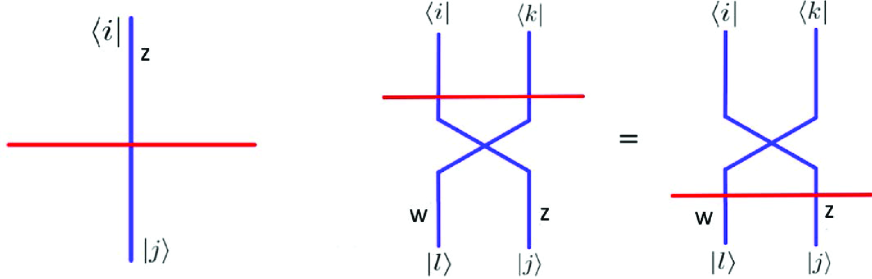
Refer to caption — Figure 1: On the left, the Lax operator $\mathcal{L}\left(z\right)$ given by the crossing of a ’t Hooft line at z=0 (in red) and a Wilson line at z (in blue) with incoming $\left\langle i\right|$ and out going $\left|j\right\rangle$ states. On the right, the RLL relations encoding the commutation relations between two L-operators at z and w.

Notice that in eq(3.11), the usual trace has been dropped out while $W_{\boldsymbol{R}}\left[\mathrm{\gamma}_{z}\right]$ still preserving gauge symmetry; this remarkable feature is due to asymptotic conditions described in [1]. Along with the line defects, one may also have their couplings given by lines’ crossings like those involved in Yang-Baxter equation (YBE). Another special type of lines crossings is given by the so-called Lax operator denoted as $\boldsymbol{L}_{(\mathbf{\hat{\mu})}}$ ; it describes the crossing of Wilson line $W_{\boldsymbol{R}}\left[\mathrm{\gamma}_{z}\right]$ by a ’t Hooft line tH ${}_{\boldsymbol{\mu}}\left[\mathrm{\gamma}_{0}\right]$ characterised by a minuscule coweight $\mathbf{\hat{\mu}}.$ An interesting realisation of this $\boldsymbol{L}_{(\mathbf{\hat{\mu})}}$ has been obtained in the CWY theory; it is given by [5],

\boldsymbol{L}_{\mathbf{\mu}}=e^{X}z^{\mathbf{\hat{\mu}}}e^{Y}

(3.12)

where $\mathbf{\hat{\mu}}$ is a minuscule coweight and X and Y are nilpotent operators of the gauge symmetry of the CWY theory. For explicit calculations regarding eq(3.12), see [19]. With this description regarding lines defects and their couplings, we complete the step-2 in the way diagram of Table 1.

4 From AdS₃ to topological 4D gravity

In this section, we carry out the third step in the way diagram of Table 1. First, we derive the field action (1.2) of the topological 4D gravity from the AdS₃ theory by implementing the building algorithm used in the derivation of the CWY theory as described above. Then, we construct gravitational line defects of the 4D topological theory and discuss their application in integrable quantum systems.

4.1 Deriving the topological 4D gravity

Following [20, 22], the AdS₃ gravity can be formulated as a difference of two Chern-Simons gauge theories. In this tricky formulation briefly revisited in section 2 as shown by eqs(2.4-2.5), the AdS₃ gravity action reads in terms of the differential- form language as the difference of two 3D CS- field actions as follows

\mathcal{S}_{3D}^{gravity}=\mathop{\displaystyle\int}\nolimits_{\mathcal{M}_{3D}}\mathcal{L}_{3}^{{\small CS}_{L}}-\mathop{\displaystyle\int}\nolimits_{\mathcal{M}_{3D}}\mathcal{L}_{3}^{{\small CS}_{R}}

(4.1)

where $\mathcal{L}_{3}^{{\small CS}_{L}}$ and $\mathcal{L}_{3}^{{\small CS}_{R}}$ are Chern-Simons 3-forms with gauge symmetries G_L and G_R.

4.1.1 Action $\mathcal{S}_{4D}^{gravity}$ in terms of CWY fields

Applying the building algorithm, used in the derivation of the CWY theory (3.5-3.10), to the 3D AdS₃ gravity action (4.1), we end up with a 4D topological gravity described by

\mathcal{S}_{4D}^{gravity}=\mathop{\displaystyle\int}\nolimits_{\boldsymbol{M}_{4D}}\mathcal{L}_{4}^{gravity}

(4.2)

with

\mathcal{L}_{4}^{gravity}=\mathcal{L}_{4}^{{\small CWY}_{L}}-\mathcal{L}_{4}^{{\small CWY}_{R}}

(4.3)

In this field action, the 4D space $\boldsymbol{M}_{4D}$ is given by the fibration $\mathbb{R}^{2}\times\mathbb{CP}^{1}$ while the left $\mathcal{L}_{4}^{{\small CWY}_{L}}$ and the right $\mathcal{L}_{4}^{{\small CWY}_{R}}$ Lagrangian 4-forms read as follows

$\mathcal{L}_{4}^{{\small CWY}_{L}}$	$=$	$dz\wedge tr\mathcal{L}_{3}^{{\small CWY}_{L}}$
$\mathcal{L}_{4}^{{\small CWY}_{R}}$	$=$	$dz\wedge tr\mathcal{L}_{3}^{{\small CWY}_{R}}$

(4.4)

with

	$\displaystyle\mathcal{L}_{3}^{{\small CWY}_{L}}$	$\displaystyle=$	$\displaystyle\boldsymbol{A}_{L}\wedge d\boldsymbol{A}_{L}+\frac{2}{3}\boldsymbol{A}_{L}\wedge\boldsymbol{A}_{L}\wedge\boldsymbol{A}_{L}$		(4.5)
	$\displaystyle\mathcal{L}_{3}^{{\small CWY}_{R}}$	$\displaystyle=$	$\displaystyle\boldsymbol{A}_{R}\wedge d\boldsymbol{A}_{R}+\frac{2}{3}\boldsymbol{A}_{R}\wedge\boldsymbol{A}_{R}\wedge\boldsymbol{A}_{R}$		(4.6)

Notice that the gauge fields $\boldsymbol{A}_{L/R}=\boldsymbol{A}_{L/R}\left(x,y,z,\bar{z}\right)$ are given by eq(3.7); i.e $\boldsymbol{A}_{L/R}=d\zeta^{\text{{a}}}A_{\text{{a}}}^{L/R}$ ; and the operator $dz\wedge$ is as in the CWY topological theory. Here, the $\boldsymbol{A}_{L}$ is valued into the Lie algebra $sl(2,\mathbb{C})_{L}$ generated by $J_{L}^{a}$ ; that is $\boldsymbol{A}_{L}=J_{a}^{L}A_{L}^{a}$ . Similarly, the $\boldsymbol{A}_{R}$ is valued into the Lie algebra $sl(2,\mathbb{C})_{R}$ generated by $J_{R}^{a}$ allowing $\boldsymbol{A}_{R}=J_{a}^{R}A_{R}^{a}.$ By performing the trace in the above relationships, we obtain

	$\displaystyle\mathcal{L}_{3}^{{\small CWY}_{L}}$	$\displaystyle=$	$\displaystyle q_{ab}\boldsymbol{A}_{L}^{a}\wedge d\boldsymbol{A}_{L}^{b}+\frac{2}{3}\varepsilon_{abc}\boldsymbol{A}_{L}^{a}\wedge\boldsymbol{A}_{L}^{b}\wedge\boldsymbol{A}_{L}^{c}$		(4.7)
	$\displaystyle\mathcal{L}_{3}^{{\small CWY}_{R}}$	$\displaystyle=$	$\displaystyle q_{ab}\boldsymbol{A}_{R}^{a}\wedge d\boldsymbol{A}_{R}^{b}+\frac{2}{3}\varepsilon_{abc}\boldsymbol{A}_{R}^{a}\wedge\boldsymbol{A}_{R}^{b}\wedge\boldsymbol{A}_{R}^{c}$		(4.8)

with Killing form $q_{ab}=Tr\left(J_{a}J_{b}\right)$ for both $sl(2,\mathbb{C})_{L}$ and $sl(2,\mathbb{C})_{R}.$ The field equation of the CWY gauge potentials 1-forms $\boldsymbol{A}_{L}$ and $\boldsymbol{A}_{R}$ are given by

	$\displaystyle\boldsymbol{H}_{3}^{L}$	$\displaystyle=$	$\displaystyle dz\wedge\boldsymbol{F}_{2}^{L}=0\,\qquad\Rightarrow\qquad\boldsymbol{F}_{2}^{L}=0$		(4.9)
	$\displaystyle\boldsymbol{H}_{3}^{R}$	$\displaystyle=$	$\displaystyle dz\wedge\boldsymbol{F}_{2}^{R}=0\,\qquad\Rightarrow\qquad\boldsymbol{F}_{2}^{R}=0$		(4.10)

where

	$\displaystyle\boldsymbol{F}_{2}^{L}$	$\displaystyle=$	$\displaystyle d\boldsymbol{A}_{L}+\boldsymbol{A}_{L}\wedge\boldsymbol{A}_{L}$		(4.11)
	$\displaystyle\boldsymbol{F}_{2}^{R}$	$\displaystyle=$	$\displaystyle d\boldsymbol{A}_{R}+\boldsymbol{A}_{R}\wedge\boldsymbol{A}_{R}$		(4.12)

The topological 4D gravity action (4.2) is one of the main results in this paper. Its explicit expression in terms of the 4D gravity 1-forms is obtained by substituting into eq(4.2) the $A_{L/R}^{a}$ by the following

$A_{L}^{a}$	$=$	$\Omega^{a}+E^{a}$
$A_{R}^{a}$	$=$	$\Omega^{a}-E^{a}$

(4.13)

They behave as 3-vectors of the complexified gauge symmetry; that is $A_{L}^{a}$ a complex triplet of $SL(2,\mathbb{C})_{L}$ while $A_{R}^{a}$ a triplet of $SL(2,\mathbb{C})_{R}$ . In this new setting, the complex potential $E^{a}$ is the 1-form dreibein expanding as $d\zeta^{\text{{a}}}E_{\text{{a}}}^{a}$ with sections $E_{\text{{a}}}^{a}=E_{\text{{a}}}^{a}\left(x,y,z,\bar{z}\right)$ living in the 4D space $\mathbb{R}^{2}\times\mathbb{CP}^{1}$ ; and the complex $\Omega^{a}$ is the l-form spin connection $d\zeta^{\text{{a}}}\Omega_{\text{{a}}}^{a}$ with components $\Omega_{\text{{a}}}^{a}=\Omega_{\text{{a}}}^{a}\left(x,y,z,\bar{z}\right)$ . For later use, we denote the two- points Green functions of these gauge fields $A_{L/R}^{a}\left(\zeta\right)=d\zeta^{\text{{a}}}A_{\text{{a}}L/R}^{a}\left(\zeta\right)$ as follows

$\left\langle A_{\text{{a}}L}^{a}\left(\zeta_{1}\right)A_{\text{{b}}L}^{b}\left(\zeta_{2}\right)\right\rangle$	$=$	$\mathcal{P}_{\text{{ab}}L}^{ab}\left(\zeta_{1}-\zeta_{2}\right)$
$\left\langle A_{\text{{a}}L}^{a}\left(\zeta_{1}\right)A_{\text{{b}}R}^{b}\left(\zeta_{2}\right)\right\rangle$	$=$	$0$
$\left\langle A_{\text{{a}}R}^{a}\left(\zeta_{1}\right)A_{\text{{b}}R}^{b}\left(\zeta_{2}\right)\right\rangle$	$=$	$\mathcal{P}_{\text{{ab}}R}^{ab}\left(\zeta_{1}-\zeta_{2}\right)$

(4.14)

where the translation invariant tensor $\mathcal{P}_{\text{{ab}}}^{ab}$ can be read from [1, 2]. Because of the minus sign in the $\mathcal{L}_{4}^{gravity}$ gravity Lagrangian given by the difference $\mathcal{L}_{4}^{{\small CWY}_{L}}-\mathcal{L}_{4}^{{\small CWY}_{R}}$ , the two-points Green functions in the right sector are related to their homologue in the left sector as

\mathcal{P}_{\text{{ab}}R}^{ab}=-\mathcal{P}_{\text{{ab}}L}^{ab}\equiv-\mathcal{P}_{\text{{ab}}}^{ab}

(4.15)

4.1.2 Action $\mathcal{S}_{4D}^{gravity}$ in terms of gravity fields

Here, we study the building of the action $\mathcal{S}_{4D}^{gravity}$ in terms of 4D gravity fields $E^{a}$ and $\Omega^{a};$ it can be obtained by substituting (4.13) into eqs (4.2-4.8). From the relations (4.13), we deduce interesting features; in particular the following two:

$\left(\mathbf{1}\right)$ The complexified 1-form spin connection $\Omega^{a}$ is related to the left and right CWY fields as the mean field of the two gauge potentials namely $(A_{L}^{a}+A_{R}^{a})/2$ ; while the complexified 1-form vielbein $E^{a}$ is given by the reduced field given by $(A_{L}^{a}-A_{R}^{a})/2$ . Notice that by putting $A_{L}^{a}=A_{R}^{a}=A^{a}$ ; then the $\left.E^{a}\right|_{A_{L}^{a}=A_{R}^{a}}$ vanishes and the spin connection $\left.\Omega^{a}\right|_{A_{L}^{a}=A_{R}^{a}}$ reduces to $A^{a}$ ; thus leading to

\left.\mathcal{L}_{4}^{{\small CWY}_{L}}\right|_{A_{L}^{a}=A_{R}^{a}}=\left.\mathcal{L}_{4}^{{\small CWY}_{R}}\right|_{A_{L}^{a}=A_{R}^{a}}

(4.16)

and consequently $\left.\mathcal{S}_{4D}^{gravity}\right|_{A_{L}^{a}=A_{R}^{a}}$ vanishes. This property indicates that the topological Lagrangian 4-form $\mathcal{L}_{4}^{gravity}(\mathbf{E},\mathbf{\Omega})$ is factorised like

\mathcal{S}_{4D}^{gravity}=\mathop{\displaystyle\int}\nolimits_{\boldsymbol{M}_{4D}}\mathcal{L}_{4}^{gravity}=\mathop{\displaystyle\int}\nolimits_{\boldsymbol{M}_{4D}}E_{a}\wedge\mathcal{K}_{3}^{a}

(4.17)

with $\mathcal{K}_{3}=\mathcal{K}_{3}(\mathbf{E},\mathbf{\Omega})$ is a 3-form function of the vielbein $\mathbf{E}$ and the spin connection $\mathbf{\Omega}$ one-forms.

$\left(\mathbf{2}\right)$ Using the operators $J^{a}=(J_{L}^{a}+J_{R}^{a})/\sqrt{2}$ generating the diagonal Lie algebra of the CS gauge symmetry namely

SL(2,\mathbb{C})_{+}=\frac{SL(2,\mathbb{C})_{L}\times SL(2,\mathbb{C})_{R}}{SL(2,\mathbb{C})_{-}}

(4.18)

one can deal with the vielbein $\mathbf{E}$ and the spin connection $\mathbf{\Omega}$ as 1-form matrices valued in $sl(2,\mathbb{C})_{+};$ thus facilitating the explicit calculations. In this formulation, the two 1-forms decompose like $\mathbf{\Omega}=\Omega^{a}J_{a}$ and $\mathbf{E}=E^{a}J_{a}$ ; which by using the Killing form $q_{ab}=tr\left(J_{a}J_{b}\right)$ , give $tr\left(J_{a}\mathbf{\Omega}\right)=q_{ab}\Omega^{b}$ and $tr\left(J_{a}\mathbf{E}\right)=q_{ab}E^{b}.$ With the help of the inverse matrix $q^{ba}$ , we also have

\Omega^{a}=q^{ab}tr\left(J_{b}\mathbf{\Omega}\right)\qquad,\qquad E^{a}=q^{ab}tr\left(J_{b}\mathbf{E}\right)

(4.19)

consequently the eq(4.17) can be rewritten as

\mathcal{S}_{4D}^{gravity}=\mathop{\displaystyle\int}\nolimits_{\boldsymbol{M}_{4D}}tr\left(\mathbf{E}\wedge\mathbf{K}_{3}\right)

(4.20)

Moreover, because of the building algorithm (3.5-3.10), the gravity 1-forms have partial expansions as follows

	$\displaystyle E^{a}$	$\displaystyle=$	$\displaystyle E_{x}^{a}dx+E_{y}^{a}dy+E_{\bar{z}}^{a}d\bar{z}$		(4.21)
	$\displaystyle\Omega^{a}$	$\displaystyle=$	$\displaystyle\Omega_{x}^{a}dx+\Omega_{y}^{a}dy+\Omega_{\bar{z}}^{a}d\bar{z}$		(4.22)

with no component $E_{z}^{a}dz$ nor $\Omega_{z}^{a}dz$ . Combining these quantities with eq(2.2), we end up with the expression of the topological 4D gravity in terms of the complexified vielbein and the spin connection namely

$\mathcal{L}_{4}^{gravity}$	$=$	$dz\wedge\left(E^{a}\wedge\boldsymbol{R}_{a}+\xi\varepsilon_{abc}E^{a}\wedge E^{b}\wedge E^{c}\right)$
$\boldsymbol{R}_{a}$	$=$	$d\Omega_{a}+\frac{1}{2}\varepsilon_{abc}\Omega^{b}\wedge\Omega^{c}$

(4.23)

In comparison with (4.17,4.20), the 3-form $\mathbf{K}_{3}$ is given by

\mathbf{K}_{3}=dz\wedge\left(\boldsymbol{R}+\xi\mathbf{E}\wedge\mathbf{E}\right)

(4.24)

Furthermore, using the formulation (4.2) of the obtained 4D topological gravity, one can compute interesting quantities characterising the $\mathcal{S}_{4D}^{grav};$ for instance, we can construct observables using the gauge $\mathbf{A}_{L}$ and $\mathbf{A}_{R}$ (or equivalently the gravitational $\mathbf{\Omega}$ and $\mathbf{E}$ ) through their gauge invariant holonomies as shown in next subsection. In due time, notice that by using the short notation $A=d\zeta^{\text{{a}}}A_{\text{{a}}}$ introduced in eq(3.7) while setting $U=d\zeta^{\text{{a}}}U_{\text{{a}}}$ and $\boldsymbol{V}=d\zeta^{\text{{a}}}V_{\text{{a}}}$ with $\boldsymbol{U}$ and $\boldsymbol{V}$ referring to $\boldsymbol{\Omega}$ and $\boldsymbol{E}$ ; then calculating their product, we obtain

\boldsymbol{UV}=\frac{1}{2}d\zeta^{\text{{b}}}\wedge d\zeta^{\text{{c}}}Z_{\text{{bc}}}\qquad,\qquad Z_{\text{{bc}}}=\left[U_{\text{{b}}},V_{\text{{c}}}\right]

(4.25)

For the case where both $\boldsymbol{U}$ and $\boldsymbol{V}$ are equal to $\mathbf{A}_{L}$ or to $\mathbf{A}_{R}$ , the commutators $\left[A_{L\text{{b}}},A_{L\text{{c}}}\right]$ and $\left[A_{R\text{{b}}},A_{R\text{{c}}}\right]$ are respectively given by $A_{L}^{b}\mathrm{f}_{bc}^{a}A_{L\text{{c}}}^{c}$ and $A_{R}^{b}\mathrm{\bar{f}}_{bc}^{a}A_{R\text{{c}}}^{c}$ with $\mathrm{f}_{bc}^{a}$ and $\mathrm{\bar{f}}_{bc}^{a}$ the complex structures of $sl(2,\mathbb{C})_{L}$ and $sl(2,\mathbb{C})_{R}.$ The commutators $\left[A_{L\text{{b}}},A_{L\text{{c}}}\right]$ and $\left[A_{R\text{{b}}},A_{R\text{{c}}}\right]$ show that traces $tr(\mathbf{A}_{L}\mathbf{A}_{L})$ and $tr(\mathbf{A}_{R}\mathbf{A}_{R})$ vanish identically because $trJ_{a}^{L}=trJ_{a}^{R}=0$ . For the case where $\boldsymbol{U}=\mathbf{A}_{L}$ and $\boldsymbol{V}=\mathbf{A}_{R}$ , the commutator $\left[A_{L\text{{b}}},A_{R\text{{c}}}\right]$ and $tr(\mathbf{A}_{L}\mathbf{A}_{R})$ vanish due to the vanishing of $[J_{La},J_{Rb}].$

Notice also that by using eq(4.13) and the property

\mathcal{P}_{\text{{ab}}L}^{ab}=+\mathcal{P}_{\text{{ab}}}^{ab}\qquad,\qquad\mathcal{P}_{\text{{ab}}R}^{ab}=-\mathcal{P}_{\text{{ab}}}^{ab}

(4.26)

we can express the Chern-Simons two-points Green functions (4.14) in terms of the two-points of the gravity fields. Straightforward calculations lead, amongst others, to the following interesting constraint relations

	$\displaystyle\left\langle E_{\text{{a}}}^{a}\left(\zeta_{1}\right)\Omega_{\text{{b}}}^{b}\left(\zeta_{2}\right)\right\rangle+\left\langle\Omega_{\text{{a}}}^{a}\left(\zeta_{1}\right)E_{\text{{b}}}^{b}\left(\zeta_{2}\right)\right\rangle$	$\displaystyle=$	$\displaystyle\mathcal{P}_{\text{{ab}}}^{ab}\left(\zeta_{1}-\zeta_{2}\right)$		(4.27)
	$\displaystyle\left\langle E_{\text{{a}}}^{a}\left(\zeta_{1}\right)\Omega_{\text{{b}}}^{b}\left(\zeta_{2}\right)\right\rangle-\left\langle\Omega_{\text{{a}}}^{a}\left(\zeta_{1}\right)E_{\text{{b}}}^{b}\left(\zeta_{2}\right)\right\rangle$	$\displaystyle=$	$\displaystyle 0$		(4.28)

As a result, the non trivial two-point Green functions of the gravity fields $E_{\text{{a}}}^{a}\left(\zeta\right)$ and $\Omega_{\text{{b}}}^{b}\left(\zeta\right)$ are given by,

$\displaystyle\left\langle E_{\text{{a}}}^{a}\left(\zeta_{1}\right)\Omega_{\text{{b}}}^{b}\left(\zeta_{2}\right)\right\rangle$	$\displaystyle=$	$\displaystyle\frac{1}{2}\mathcal{P}_{\text{{ab}}}^{ab}\left(\zeta_{1}-\zeta_{2}\right)$	(4.29)
$\displaystyle\left\langle\Omega_{\text{{a}}}^{a}\left(\zeta_{1}\right)\Omega_{\text{{b}}}^{b}\left(\zeta_{2}\right)\right\rangle$	$\displaystyle=$	$\displaystyle 0$	(4.30)
$\displaystyle\left\langle E_{\text{{a}}}^{a}\left(\zeta_{1}\right)E_{\text{{b}}}^{b}\left(\zeta_{2}\right)\right\rangle$	$\displaystyle=$	$\displaystyle 0$	(4.31)

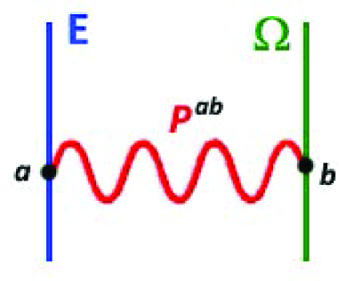
A graphical description of the above propagator is illustrated in the Figure 2 where a vielbein line defect $\boldsymbol{E}^{a}$ at $\zeta_{1}$ exchanges a topological graviton with a spin connection line defect $\boldsymbol{\Omega}^{a}$ at $\zeta_{2}$ .

Using the 1-forms $\boldsymbol{E}^{a}=d\zeta^{\text{{a}}}E_{\text{{a}}}^{a}$ and $\boldsymbol{\Omega}^{a}=d\zeta^{\text{{a}}}\Omega_{\text{{a}}}^{a}$ as well as the 2-form,

\mathcal{P}^{ab}\left(\zeta\right)=\frac{1}{2}d\zeta^{\text{{a}}}\wedge d\zeta^{\text{{b}}}\mathcal{P}_{\text{{ab}}}^{ab}\left(\zeta\right)

(4.32)

we can present the gravitational two-points Green functions (4.29-4.31) in a shortened form as follows

\left\langle\boldsymbol{E}^{a}\left(\zeta_{1}\right)\boldsymbol{\Omega}^{b}\left(\zeta_{2}\right)\right\rangle=\mathcal{P}^{ab}\left(\zeta_{1}-\zeta_{2}\right)

(4.33)

and

\left\langle\boldsymbol{E}^{a}\left(\zeta_{1}\right)\boldsymbol{E}^{b}\left(\zeta_{2}\right)\right\rangle=\left\langle\boldsymbol{\Omega}^{a}\left(\zeta_{1}\right)\boldsymbol{\Omega}^{b}\left(\zeta_{2}\right)\right\rangle=0

(4.34)

where $\mathcal{P}^{ab}\left(\zeta\right)=\delta^{ab}\mathcal{P}\left(\zeta\right)$ with scalar 2-form,

\mathcal{P}\left(\zeta\right)=\frac{1}{2\pi\left(x^{2}+y^{2}+\zeta\bar{\zeta}\right)^{2}}\left(xdy\wedge d\zeta+yd\bar{\zeta}\wedge dx+2\zeta dx\wedge dy\right)

(4.35)

The vanishing propagators $\left\langle\boldsymbol{E}\left(\zeta_{1}\right)\boldsymbol{E}\left(\zeta_{2}\right)\right\rangle$ and $\left\langle\boldsymbol{\Omega}\left(\zeta_{1}\right)\boldsymbol{\Omega}\left(\zeta_{2}\right)\right\rangle$ given by (4.30-4.31) show that identical topological gravitational line defects cannot interact directly; they must couple either indirectly via a different topological defect as exhibited by the Figure 3,

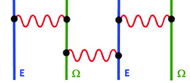
or via quantum corrections.

4.2 Line defects in 4D topological gravity

Because of the flatness of the gauge curvatures (4.9-4.10), no gauge invariant observable can be built out of the gauge 2-forms $\boldsymbol{F}_{2}^{L}$ and $\boldsymbol{F}_{2}^{R}$ as they vanish on shell. Observables in this 4D topological gravity are given by surface and line defects [14, 15] sitting in $\mathbb{R}^{2}\times\mathbb{CP}^{1}$ ; they are obtained by extending results from the CWY theory while using the loop matrices

\Phi_{\boldsymbol{A}_{L}}\left[\mathrm{\gamma}_{z}\right]=\mathop{\displaystyle\oint}\nolimits_{\mathrm{\gamma}_{z}}\boldsymbol{A}_{L}\qquad,\qquad\Phi_{\boldsymbol{A}_{R}}\left[\mathrm{\gamma}_{z}\right]=\mathop{\displaystyle\oint}\nolimits_{\mathrm{\gamma}_{z}}\boldsymbol{A}_{R}

(4.36)

with $\Phi_{\boldsymbol{A}_{L}/\boldsymbol{A}_{R}}$ valued in $sl(2,\mathbb{C})_{L/R}.$

4.2.1 Gravitational holonomies

The above loop matrices are gauge holonomies of the topological CS fields $\boldsymbol{A}_{L}$ and $\boldsymbol{A}_{R}.$ With the help of the change (4.13), we can also express these gravitational holonomies of 4D gravity in terms of the gravitational 1-form potentials as follows

\Phi_{\Omega}\left[\mathrm{\gamma}_{z}\right]=\mathop{\displaystyle\oint}\nolimits_{\mathrm{\gamma}_{z}}\boldsymbol{\Omega}\qquad,\qquad\Phi_{E}\left[\mathrm{\gamma}_{w}\right]=\mathop{\displaystyle\oint}\nolimits_{\mathrm{\gamma}_{w}}\boldsymbol{E}

(4.37)

These novel loop matrices are valued in $sl(2,\mathbb{C})$ given by eq(4.18) and generated by the diagonal $J_{a}$ s; they define the gravitational holonomies in opposition to the gauge holonomies (4.36). Notice that as in eq(4.36), the real lines $\mathrm{\gamma}_{z}$ and $\mathrm{\gamma}_{w}$ appearing (4.37) are loops spreading in $\mathbb{R}^{2}$ ; but sitting at the point z and w in the complex projective line $\mathbb{CP}^{1}$ . These loop matrices are given by eq(1.3); because $\mathrm{\gamma}_{z}$ and $\mathrm{\gamma}_{w}$ spread in the topological plane $\mathbb{R}^{2}$ , they read explicitly as follows

	$\displaystyle\Phi_{E}{\small[}\mathrm{\gamma}_{z}{\small]}$	$\displaystyle=$	$\displaystyle\mathop{\displaystyle\oint}\nolimits_{\mathrm{\gamma}_{z}}\left(\mathbf{E}_{x}dx+\mathbf{E}_{y}dy\right)$		(4.38)
	$\displaystyle\Phi_{\Omega}{\small[}\mathrm{\gamma}_{w}{\small]}$	$\displaystyle=$	$\displaystyle\mathop{\displaystyle\oint}\nolimits_{\mathrm{\gamma}_{w}}\left(\mathbf{\Omega}_{x}dx+\mathbf{\Omega}_{y}dy\right)$		(4.39)

Using $\boldsymbol{A}_{L}=J_{a}^{L}A_{L}^{a}$ and $\boldsymbol{A}_{R}=J_{a}^{R}A_{R}^{a}$ as well as $\mathbf{E}=J_{a}E^{a}$ and $\mathbf{\Omega}=J_{a}\Omega^{a},$ the gauge and gravity loop matrices expand like

$\Phi_{\boldsymbol{A}_{L}}\left[\mathrm{\gamma}_{z}\right]$	$=$	$J_{a}^{L}\Phi_{\boldsymbol{A}_{L}}^{a}{\small[}\mathrm{\gamma}_{z}{\small]}$
$\Phi_{\boldsymbol{A}_{R}}\left[\mathrm{\gamma}_{z}\right]$	$=$	$J_{a}^{R}\Phi_{\boldsymbol{A}_{R}}^{a}{\small[}\mathrm{\gamma}_{z}{\small]}$
$\Phi_{E}{\small[}\mathrm{\gamma}_{z}{\small]}$	$=$	$J_{a}\Phi_{E}^{a}{\small[}\mathrm{\gamma}_{z}{\small]}$
$\Phi_{\Omega}{\small[}\mathrm{\gamma}_{z}{\small]}$	$=$	$J_{a}\Phi_{\Omega}^{a}{\small[}\mathrm{\gamma}_{z}{\small]}$

(4.40)

with components as

$\Phi_{\boldsymbol{A}_{L}}^{a}\left[\mathrm{\gamma}_{z}\right]$	$=$	$\mathop{\displaystyle\oint}\nolimits_{\mathrm{\gamma}_{z}}\boldsymbol{A}_{L}^{a}$
$\Phi_{\boldsymbol{A}_{R}}^{a}\left[\mathrm{\gamma}_{z}\right]$	$=$	$\mathop{\displaystyle\oint}\nolimits_{\mathrm{\gamma}_{z}}\boldsymbol{A}_{R}^{a}$
$\Phi_{\Omega}^{a}\left[\mathrm{\gamma}_{z}\right]$	$=$	$\mathop{\displaystyle\oint}\nolimits_{\mathrm{\gamma}_{z}}\boldsymbol{\Omega}^{a}$
$\Phi_{E}^{a}\left[\mathrm{\gamma}_{z}\right]$	$=$	$\mathop{\displaystyle\oint}\nolimits_{\mathrm{\gamma}_{z}}\boldsymbol{E}^{a}$

(4.41)

These holonomy components follow from the projections

$\Phi_{\boldsymbol{A}_{L/R}}^{a}$	$=$	$q_{L/R}^{ab}tr(J_{b}^{L/R}\Phi_{\boldsymbol{A}_{L/R}})$
$\Phi_{\boldsymbol{\Omega}}^{a}$	$=$	$q^{ab}tr(J_{b}\Phi_{\boldsymbol{\Omega}})$
$\Phi_{\boldsymbol{E}}^{a}$	$=$	$q^{ab}tr(J_{b}\Phi_{\boldsymbol{E}})$

(4.42)

with $q_{ab}^{L/R}=tr(J_{a}^{L/R}J_{b}^{L/R})$ and $q_{L/R}^{ab}$ its inverse $q_{L/R}^{ba}$ . The gravitational loop matrices (4.40) satisfy the commutation property

\Phi_{\boldsymbol{A}_{L}}{\small[}\mathrm{\gamma}_{z}{\small]}\bullet\Phi_{\boldsymbol{A}_{R}}{\small[}\mathrm{\gamma}_{z}{\small]}=\Phi_{\boldsymbol{A}_{R}}{\small[}\mathrm{\gamma}_{z}{\small]}\bullet\Phi_{\boldsymbol{A}_{L}}{\small[}\mathrm{\gamma}_{z}{\small]}

(4.43)

as well as the non commutation relations

\Phi_{\Omega}{\small[}\mathrm{\gamma}_{z}{\small]}\bullet\Phi_{E}{\small[}\mathrm{\gamma}_{z}{\small]}-\Phi_{E}{\small[}\mathrm{\gamma}_{z}{\small]}\bullet\Phi_{\Omega}{\small[}\mathrm{\gamma}_{z}{\small]}=\Psi_{\Omega E}{\small[}\mathrm{\gamma}_{z}{\small]}

(4.44)

with

\Psi_{\Omega E}{\small[}\mathrm{\gamma}_{z}{\small]}=J_{a}\Psi_{\Omega E}^{a}{\small[}\mathrm{\gamma}_{z}{\small]}

(4.45)

and

(\Psi_{\Omega E}{\small[}\mathrm{\gamma}_{z}{\small])}_{a}=\varepsilon_{abc}\Phi_{\Omega}^{b}{\small[}\mathrm{\gamma}_{z}{\small]}\Phi_{E}^{c}{\small[}\mathrm{\gamma}_{z}{\small]}

(4.46)

By using eq(4.13), we have the relationships

$\Phi_{\boldsymbol{A}_{L}}^{a}\left[\mathrm{\gamma}_{z}\right]$	$=$	$\Phi_{\Omega}^{a}\left[\mathrm{\gamma}_{z}\right]+\Phi_{\boldsymbol{E}}^{a}\left[\mathrm{\gamma}_{z}\right]$
$\Phi_{\boldsymbol{A}_{R}}^{a}\left[\mathrm{\gamma}_{z}\right]$	$=$	$\Phi_{\Omega}^{a}\left[\mathrm{\gamma}_{z}\right]-\Phi_{\boldsymbol{E}}^{a}\left[\mathrm{\gamma}_{z}\right]$
$\Phi_{\Omega}^{a}\left[\mathrm{\gamma}_{z}\right]$	$=$	$\frac{1}{2}\left(\Phi_{\boldsymbol{A}_{L}}^{a}\left[\mathrm{\gamma}_{z}\right]+\Phi_{\boldsymbol{A}_{R}}^{a}\left[\mathrm{\gamma}_{z}\right]\right)$
$\Phi_{\boldsymbol{E}}^{a}\left[\mathrm{\gamma}_{z}\right]$	$=$	$\frac{1}{2}\left(\Phi_{\boldsymbol{A}_{L}}^{a}\left[\mathrm{\gamma}_{z}\right]-\Phi_{\boldsymbol{A}_{R}}^{a}\left[\mathrm{\gamma}_{z}\right]\right)$

(4.47)

leading to

	$\displaystyle\Phi_{\Omega}^{a}\left[\mathrm{\gamma}_{z}\right]$	$\displaystyle=$	$\displaystyle\frac{q^{ab}}{2}\left[tr(J_{b}^{L}\Phi_{\boldsymbol{A}_{L}}\left[\mathrm{\gamma}_{z}\right])+tr(J_{b}^{R}\Phi_{\boldsymbol{A}_{R}}\left[\mathrm{\gamma}_{z}\right])\right]$		(4.48)
	$\displaystyle\Phi_{E}^{a}\left[\mathrm{\gamma}_{z}\right]$	$\displaystyle=$	$\displaystyle\frac{q^{ab}}{2}\left[tr(J_{b}^{L}\Phi_{\boldsymbol{A}_{L}}\left[\mathrm{\gamma}_{z}\right])-tr(J_{b}^{R}\Phi_{\boldsymbol{A}_{R}}\left[\mathrm{\gamma}_{z}\right])\right]$		(4.49)

where we have used $q_{L}^{ab}=q_{R}^{ab}=q^{ab}$ . By setting

tr(J_{a}J_{b}^{L})=\chi_{ab}^{L}\qquad,\qquad tr(J_{a}J_{b}^{R})=\chi_{ab}^{R}

(4.50)

they read as follows

	$\displaystyle\Phi_{\Omega}^{a}\left[\mathrm{\gamma}_{z}\right]$	$\displaystyle=$	$\displaystyle\frac{q^{ab}}{2}\left(\chi_{bc}^{L}\Phi_{\boldsymbol{A}_{L}}^{c}\left[\mathrm{\gamma}_{z}\right]+\chi_{bc}^{R}\Phi_{\boldsymbol{A}_{R}}^{c}\left[\mathrm{\gamma}_{z}\right]\right)$		(4.51)
	$\displaystyle\Phi_{E}^{a}\left[\mathrm{\gamma}_{z}\right]$	$\displaystyle=$	$\displaystyle\frac{q^{ab}}{2}\left(\chi_{bc}^{L}\Phi_{\boldsymbol{A}_{L}}^{c}\left[\mathrm{\gamma}_{z}\right]-\chi_{bc}^{R}\Phi_{\boldsymbol{A}_{R}}^{c}\left[\mathrm{\gamma}_{z}\right]\right)$		(4.52)

By using $\chi_{bc}^{L}=\chi_{bc}^{R}=q_{bc}$ , we bring the above relations to a simpler form

	$\displaystyle\Phi_{\Omega}^{a}\left[\mathrm{\gamma}_{z}\right]$	$\displaystyle=$	$\displaystyle\frac{1}{2}\left(\Phi_{\boldsymbol{A}_{L}}^{a}\left[\mathrm{\gamma}_{z}\right]+\Phi_{\boldsymbol{A}_{R}}^{a}\left[\mathrm{\gamma}_{z}\right]\right)$		(4.53)
	$\displaystyle\Phi_{E}^{a}\left[\mathrm{\gamma}_{z}\right]$	$\displaystyle=$	$\displaystyle\frac{1}{2}\left(\Phi_{\boldsymbol{A}_{L}}^{a}\left[\mathrm{\gamma}_{z}\right]-\Phi_{\boldsymbol{A}_{R}}^{a}\left[\mathrm{\gamma}_{z}\right]\right)$		(4.54)

showing that gravitational holonomies $\Phi_{\Omega}^{a}\left[\mathrm{\gamma}_{z}\right]$ and $\Phi_{E}^{a}\left[\mathrm{\gamma}_{z}\right]$ are given by linear combinations of the left/right gauge holonomies $\Phi_{\boldsymbol{A}_{L}}^{a}$ and $\Phi_{\boldsymbol{A}_{R}}^{a}$ used in eq(3.11). The $\Phi_{\Omega}^{a}\left[\mathrm{\gamma}_{z}\right]$ is the mean value of $\Phi_{\boldsymbol{A}_{L}}^{a}\left[\mathrm{\gamma}_{z}\right]$ and $\Phi_{\boldsymbol{A}_{R}}^{a}\left[\mathrm{\gamma}_{z}\right]$ while the $\Phi_{E}^{a}\left[\mathrm{\gamma}_{z}\right]$ is the relative —reduced— value.

Moreover using line defects of the CWY theory such as the Wilson loops (3.11), we see that due to eqs(4.2-4.6), they appear in both varieties left $W_{\boldsymbol{A}_{L}}\left[\mathrm{\gamma}_{z}\right]$ and right $W_{\boldsymbol{A}_{R}}\left[\mathrm{\gamma}_{z}\right]$ given by

	$\displaystyle W_{\boldsymbol{A}_{L}}\left[\mathrm{\gamma}_{z}\right]$	$\displaystyle=$	$\displaystyle Pe^{\Phi_{A_{L}}\left[\mathrm{\gamma}_{z}\right]}$		(4.55)
	$\displaystyle W_{\boldsymbol{A}_{R}}\left[\mathrm{\gamma}_{z}\right]$	$\displaystyle=$	$\displaystyle Pe^{\Phi_{A_{R}}\left[\mathrm{\gamma}_{z}\right]}$		(4.56)

By using eq(4.13), these topological gauge lines can be presented in terms of gravitational defects $W_{E}\left[\mathrm{\gamma}_{z}\right]$ and $W_{\Omega}\left[\mathrm{\gamma}_{z}\right]$ like

	$\displaystyle W_{\boldsymbol{A}_{L}}\left[\mathrm{\gamma}_{z}\right]$	$\displaystyle=$	$\displaystyle P\exp\left(\mathop{\displaystyle\oint}\nolimits_{\mathrm{\gamma}_{z}}\Omega+\mathop{\displaystyle\oint}\nolimits_{\mathrm{\gamma}_{z}}E\right)$		(4.57)
	$\displaystyle W_{\boldsymbol{A}_{R}}\left[\mathrm{\gamma}_{w}\right]$	$\displaystyle=$	$\displaystyle P\exp\left(\mathop{\displaystyle\oint}\nolimits_{\mathrm{\gamma}_{z}}\Omega-\mathop{\displaystyle\oint}\nolimits_{\mathrm{\gamma}_{z}}E\right)$		(4.58)

These relations show that in the 4D topological gravity (4.2), one distinguishes two non commuting gravitational Wilson-like lines $W_{E}\left[\mathrm{\gamma}_{z}\right]$ and $W_{\Omega}\left[\mathrm{\gamma}_{z}\right]$ defined as

	$\displaystyle W_{E}\left[\mathrm{\gamma}_{z}\right]$	$\displaystyle=$	$\displaystyle P\exp\left(\mathop{\displaystyle\oint}\nolimits_{\mathrm{\gamma}_{z}}\mathbf{E}\right)$		(4.59)
	$\displaystyle W_{\Omega}\left[\mathrm{\gamma}_{z}\right]$	$\displaystyle=$	$\displaystyle P\exp\left(\mathop{\displaystyle\oint}\nolimits_{\mathrm{\gamma}_{z}}\mathbf{\Omega}\right)$		(4.60)

These gravitational line defects give basic topological observables that constitute building blocks towards the study of quantum integrability in the obtained 4D topological gravity.

Other basic building blocks will be given below.

4.2.2 Gravitational integrable equations

Applications of the gravitational line defects constructed above to quantum integrable systems and brane realisations in type II strings along the line of [18] will be given in a future occasion. Below, we give partial results by considering below two particular systems of crossing line defects.

A) gravitational Yang-Baxter like system
Here, we give two examples of integrable relations having a description in terms of crossing gravitational line defects (4.59-4.60). The first example we give concerns the gravitational Yang-Baxter like equation; it is represented graphically by the Figure 4. It is given by a set of 2+2 non trivial crossings of topological line defects involving:

$\left(\mathbf{a}\right)$: two Wilson line defects of vielbein like W_E[ $\mathrm{\gamma}_{z_{1}}{\small]}$ and W_E[ $\mathrm{\gamma}_{z_{2}}{\small]}$ ; they are given by the lines $\mathrm{\gamma}_{z_{1}}$ and $\mathrm{\gamma}_{z_{2}}$ spreading in the topological plane $\mathbb{R}^{2}$ ; and respectively located at $z_{1}$ and $z_{2}$ in the holomorphic $\mathbb{CP}^{1}{\small.}$
$\left(\mathbf{b}\right)$: two Wilson line defects of spin connection like W_Ω[ $\mathrm{\xi}_{w_{3}}{\small]},$ W_Ω[ $\mathrm{\xi}_{w_{4}}{\small]}$ ; they are given by the lines $\mathrm{\xi}_{w_{3}}$ and $\mathrm{\xi}_{w_{4}}$ spreading in $\mathbb{R}^{2}$ and located at $w_{3}$ and $w_{4}$ .

The positions of these gravitational topological lines in the plane $\mathbb{R}^{2}$ are such that they have crossings as depicted by the Figure 3. This particular configuration of four lines have three intersection points given by

$P_{13}$	$=$	$\mathrm{\gamma}_{z_{1}}\cap\mathrm{\xi}_{w_{3}}$
$P_{14}$	$=$	$\mathrm{\gamma}_{z_{1}}\cap\mathrm{\xi}_{w_{4}}$
$P_{23}$	$=$	$\mathrm{\gamma}_{z_{2}}\cap\mathrm{\xi}_{w_{3}}$

(4.61)

but no intersection point $P_{24}$ because W_E[ $\mathrm{\gamma}_{z_{2}}{\small]}$ and W_Ω[ $\mathrm{\xi}_{w_{3}}{\small]}$ are parallel. Then, we use the topological symmetry in the topological $\mathbb{R}^{2}$ to move the two vertical line defects W_E[ $\mathrm{\gamma}_{z_{2}}{\small]}$ and W_Ω[ $\mathrm{\xi}_{w_{3}}{\small]}$ from the left side of the node $\mathbf{R}_{14}$ to the right side. This shifting process in $\mathbb{R}^{2}$ generates the integrability equations

\mathbf{R}_{13}\otimes\mathbf{R}_{14}\otimes\mathbf{R}_{24}=\mathbf{R}_{24}\otimes\mathbf{R}_{14}\otimes\mathbf{R}_{13}

(4.62)

with $z_{ij}=z_{i}-z_{j}$ ; and where $\mathbf{R}_{ij}=\mathbf{R}\left(z_{ij}\right)$ is the Yang-Baxter R-matrix of integrable quantum systems [1] acting in the tensor space

V_{1}\otimes V_{2}\otimes V_{3}\otimes V_{4}

(4.63)

A semi classical expression of $\mathbf{R}_{ij}$ is given by

\mathbf{R}_{\text{{ab}}}^{\text{{cd}}}\left(z_{i}-z_{j}\right)=\delta_{\text{{a}}}^{\text{{c}}}\delta_{\text{{b}}}^{\text{{d}}}+\frac{\hbar}{z_{i}-z_{j}}\mathbf{c}_{\text{{ab}}}^{\text{{cd}}}+O\left(\hbar^{2}\right)

(4.64)

where $\mathbf{c}_{\text{{ab}}}^{\text{{cd}}}$ stands for the double Casimir of the gauge symmetry; its value for $sl\left(N,\mathbb{C}\right)$ is $\delta_{\text{{a}}}^{\text{{c}}}\delta_{\text{{b}}}^{\text{{d}}}.$ The second example we give involves the crossings of three topological lines; this system can be: $\left(i\right)$ completely trivial as for the cases where the three lines are of same nature; that is having the same color; or $\left(ii\right)$ lead to commutative products as for the situation depicted by the the Figure 5.

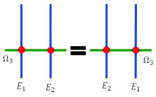
For this line system, the obtained integrability equation leads the following commutation relation resulting from the move of the line E1 from the left to the right of the line E2,

\mathbf{R}_{13}\otimes\mathbf{R}_{23}=\mathbf{R}_{23}\otimes\mathbf{R}_{13}

(4.65)

B) gravitational RLL- like system
This is an interesting system of topological 4D gravity generalising the usual RLL relations in the CWY gauge theory depicted by the Figure 1-(b). It involves a set of 2+2 non trivial crossings of topological line defects as described here below:

$\left(\mathbf{\alpha}\right)$: two Wilson-like lines W_E[ $\mathrm{\gamma}_{z_{1}}{\small]},$ W ${}_{\Omega_{2}}$ [ $\mathrm{\xi}_{w_{2}}{\small]}$ with quantum states respectively characterised by highest weights (HW) $\boldsymbol{e}$ and $\boldsymbol{\lambda}$ of the gauge symmetry —here SL(2, $\mathbb{C}$ )—. These two HWs can be taken equal.
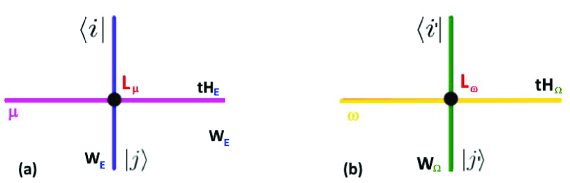
$\left(\mathbf{\beta}\right)$: two dual line defects described by ’t Hooft lines tH_E[ $\mathrm{\gamma}_{z_{3}}{\small]}$ and tH_Ω[ $\mathrm{\xi}_{w_{4}}{\small]}$ .

Figure 6: ’t Hooft lines tH_μ and tH_ω respectively dual to the Wilson lines W_E and W_Ω. On the left the vielbein pair given by a horizontal magenta ’t Hooft line dual to vertical blue Wilson line line On the right the spin connection pair given by a horizontal yellow t Hooft line dual to vertical green Wilson line.

These ’t Hooft lines are characterised by coweights $\mu$ and $\omega$ respectively dual to the weights $\boldsymbol{e}$ and $\boldsymbol{\lambda}$ . These ’t Hooft lines are depicted by the red and the Yellow lines in the Figure 6.

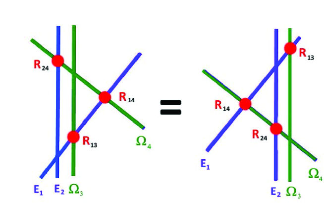
Using the gravitational Wilson-like lines W_E[ $\mathrm{\gamma}_{z_{1}}{\small]},$ W ${}_{\Omega_{2}}$ [ $\mathrm{\xi}_{w_{2}}{\small]}$ and their magnetic duals tH_E[ $\mathrm{\gamma}_{z_{3}}{\small]},$ tH_Ω[ $\mathrm{\xi}_{w_{4}}{\small]}$ all of them spreading in the topological plane with intersections as depicted by the Figure 7,

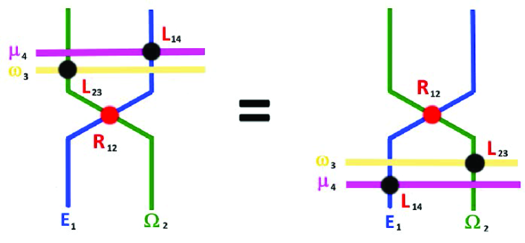
one can derive the integrability equation describing the solvability of this gravitational system. Indeed, starting from the left side in the Figure 7 with horizontal ’t Hooft lines (in yellow and magenta colors); then moving these two horizontal lines below the vertex $\mathbf{R}_{12}$ , we obtain the gravitational RLL- like in topological 4D gravity. It reads formally as

\mathbf{R}_{12}\otimes\mathbf{L}_{23}\otimes\mathbf{L}_{14}=\mathbf{L}_{14}\otimes\mathbf{L}_{23}\otimes\mathbf{R}_{12}

(4.66)

where $\mathbf{L}_{14}$ and $\mathbf{L}_{23}$ are Lax operators whose expressions can be obtained by using the formula eq(3.12), for technical computations of the $\mathbf{L}_{ij}$ ’s in CWY theory see [19]. The explicit expression of the integrability relation (4.66) reads as follows

\mathbf{R}_{\text{{ef}}}^{\text{{ad}}}\left(z_{1}-z_{2}\right)\mathbf{L}_{\text{{b}}}^{\text{{e}}}\left(z_{1}\right)\mathbf{L}_{\text{{c}}}^{\text{{f}}}\left(z_{2}\right)=\mathbf{L}_{\text{{e}}}^{\text{{a}}}\left(z_{2}\right)\mathbf{L}_{\text{{f}}}^{\text{{d}}}\left(z_{1}\right)\mathbf{R}_{\text{{ad}}}^{\text{{ef}}}\left(z_{1}-z_{2}\right)

(4.67)

5 Conclusion and comments

In this study, we have constructed a novel integrable 4D topological gravity obtained by extending the CWY method, used in the derivation of the so-called 4D Chern-Simons of integrable spin chains, to the 3D Anti de Sitter gravity. Here, the CWY method has been applied to the AdS₃ gravity; thus leading to an emergent 4D topological gravity with observables given by topological gravitational defects. Concretely, the field action $\mathcal{S}_{4D}^{grav}$ of the obtained 4D gravity is given by eqs(4.2-4.6) or equivalently by (4.23);

\mathcal{S}_{4D}^{gravity}=\mathop{\displaystyle\int}\nolimits_{R^{2}\times\mathbb{CP}^{1}}dz\wedge E^{a}\wedge\left(d\Omega_{a}+\frac{1}{2}\varepsilon_{abc}\Omega^{b}\wedge\Omega^{c}+\xi\varepsilon_{abc}E^{b}\wedge E^{c}\right)

(5.1)

It has been obtained by using the Chern-Simons formulation of AdS₃ gravity as shown by eqs (2.4) and (4.1). Moreover, because $\mathcal{S}_{AdS_{3}}^{grav}$ is formulated in terms of two copies of Chern-Simons fields $A_{L}$ and $A_{R}$ , we ended up with two particular gravitational lines defects $W_{E}\left[\mathrm{\gamma}_{z}\right]$ and $W_{\Omega}\left[\mathrm{\gamma}_{z}\right]$ respectively termed as vielbein and spin connection lines. These line defects are given by eqs(4.57-4.60) and were used to derive partial results regarding their crossings. Applications of this construction in quantum integrability and embeddings in string theory as well as in link with BTZ black-hole will be considered in a future occasion.

In the end of this investigation, we want to make a comment regarding the extension of the AdS₃/CFT₂ correspondence. Applying the AdS/CFT duality to the CWY theory, one expects to have an emergent 4D bulk/3D edge correspondence for topological 4D gravity. Below, we give an argument indicating that this emergent 4D bulk/3D edge constitute an interesting example of Gravity/Gauge duality where $\left(i\right)$ the gravity sector is given by the obtained topological 4D gravity described by the field action $\mathcal{S}_{4D}^{gravity}$ (5.1); and $\left(ii\right)$ the gauge sector is given by the topological 3D Chern-Simons with field action $\mathcal{S}_{3D}^{{\small CS}}$ as in (3.1). Indeed, in this conjectured 4D/3D correspondence, gravitational line defects $\mathrm{\gamma}_{z}$ spreading in the $\mathbb{R}^{2}$ plane of the 4D space $\boldsymbol{M}_{4}=\mathbb{R}^{2}\times\mathbb{CP}^{1}$ gets mapped into point-like particles on the 3D boundary

\partial\boldsymbol{M}_{4}=\left(\partial\mathbb{R}^{2}\right)\times\mathbb{CP}^{1}\qquad,\qquad\partial\left(\mathbb{CP}^{1}\right)=\emptyset

(5.2)

Because $\mathcal{S}_{4D}^{gravity}$ on $\boldsymbol{M}_{4}$ is topological, the dual gauge theory on $\partial\boldsymbol{M}_{4}=\boldsymbol{M}_{3}$ should be topological; thus justifying the $\mathcal{S}_{3D}^{{\small CS}}$ on the 3D boundary. This 4D/3D duality can be made more explicit by thinking about the topological plane $\mathbb{R}^{2}$ in terms of the fibration $\mathbb{R}_{>0}\times\mathbb{S}^{1}$ with $\left(\partial\mathbb{R}^{2}\right)\sim\mathbb{S}^{1}$ ; then the 3D boundary $\partial\boldsymbol{M}_{4}$ is given by $\mathbb{S}^{1}\times\mathbb{S}^{2}$ which is isomorphic to a 3-sphere $\mathbb{S}^{3}.$ Within this view, we see that

\mathbb{R}^{2}\times\mathbb{CP}^{1}\sim\mathbb{R}_{>0}\times\mathbb{S}^{3}

(5.3)

and consequently gravitational line defects $\mathrm{\gamma}_{z}$ spreading in $\mathbb{R}^{2}$ are dual to particle states on the 3-sphere. Notice also that for the elliptic case where $\boldsymbol{M}_{4}=\mathbb{R}^{2}\times\mathbb{T}^{2}$ ; the 3D boundary has a $\mathbb{T}^{3}$ geometry; then the dual CS gauge theory lives on a 3-torus. Progress in this direction will be reported in a future occasion.

References

[1] Costello, K., Witten, E., & Yamazaki, M. (2017). Gauge theory and integrability, I. arXiv preprint arXiv:1709.09993.
[2] Costello, K., Witten, E., & Yamazaki, M. (2018). Gauge theory and integrability, II. arXiv preprint arXiv:1802.01579.
[3] Costello, K., & Stefański Jr, B. (2020). Chern-Simons origin of superstring integrability. Physical Review Letters, 125(12), 121602.
[4] Costello, K., & Yamazaki, M. (2019). Gauge theory and integrability, III. arXiv preprint arXiv:1908.02289.
[5] Costello, K., Gaiotto, D., & Yagi, J. (2021). Q-operators are’t Hooft lines. arXiv preprint arXiv:2103.01835.
[6] Retore, A. L. (2022). Introduction to classical and quantum integrability. Journal of Physics A: Mathematical and Theoretical, 55(17), 173001.
[7] Lacroix, S. (2022). Four-dimensional Chern–Simons theory and integrable field theories. Journal of Physics A: Mathematical and Theoretical, 55(8), 083001.
[8] Liniado, J., & Vicedo, B. (2023, October). Integrable Degenerate E-Models from 4d Chern–Simons Theory. In Annales Henri Poincare (Vol. 24, No. 10, pp. 3421-3459). Cham: Springer International Publishing.
[9] Khan, A. Z. (2022). Holomorphic Surface Defects in Four-Dimensional Chern-Simons Theory. arXiv preprint arXiv:2209.07387.
[10] Ashwinkumar, M. (2021). Integrable lattice models and holography. Journal of High Energy Physics, 2021(2), 1-22.
[11] Ashwinkumar, M., Tan, M. C., & Zhao, Q. (2018). Branes and categorifying integrable lattice models. arXiv preprint arXiv:1806.02821.
[12] Ashwinkumar, M., & Tan, M. C. (2019). Unifying lattice models, links and quantum geometric Langlands via branes in string theory. arXiv preprint arXiv:1910.01134.
[13] Fukushima, O., Sakamoto, J. I., & Yoshida, K. (2021). Faddeev-Reshetikhin model from a 4D Chern-Simons theory. Journal of High Energy Physics, 2021(2), 1-18. arXiv:2012.07370v1 [hep-th].
[14] Saidi, E. H. (2020). Quantum line operators from Lax pairs. Journal of Mathematical Physics, 61(6).
[15] Maruyoshi, K., Ota, T., & Yagi, J. (2021). Wilson-’t Hooft lines as transfer matrices. Journal of High Energy Physics, 2021(1), 1-31.
[16] Bazhanov, V. V., Frassek, R., Łukowski, T., Meneghelli, C., & Staudacher, M. (2011). Baxter Q-operators and representations of Yangians. Nuclear Physics B, 850(1), 148-174.
[17] Ishtiaque, N., Moosavian, S. F., Raghavendran, S., & Yagi, J. (2022). Superspin chains from superstring theory. SciPost Physics, 13(4), 083.
[18] Boujakhrout, Y., Saidi, E. H., Laamara, R. A., & Drissi, L. B. (2023). Embedding integrable superspin chain in string theory. Nuclear Physics B, 990, 116156.
[19] Boujakhrout, Y., Saidi, E. H., Ahl Laamara, R., & Btissam Drissi, L. (2023). ’t Hooft lines of ADE-type and topological quivers. SciPost Physics, 15(3), 078.
[20] Achucarro, A., & Townsend, P. K. (1986). A Chern-Simons action for three-dimensional anti-de Sitter supergravity theories. Physics Letters B, 180(1-2), 89-92.
[21] Avery, S. G., Poojary, R. R., & Suryanarayana, N. V. (2014). An sl (2, $\mathbb{R}$ ) current algebra from AdS 3 gravity. Journal of High Energy Physics, 2014(1), 1-9.
[22] Castro, A. (2016). Lectures on higher spin black holes in AdS3 gravity. Acta Phys. Polon. B, 47, 2479.
[23] Sammani, R., Boujakhrout, Y., Saidi, E. H., Laamara, R. A., & Drissi, L. B. (2023). Swampland constraints on higher spin AdS ₃ gravity Landscape. arXiv preprint arXiv:2304.01887.
[24] Sammani, R., Boujakhrout, Y., Saidi, E. H., Laamara, R. A., & Drissi, L. B. (2023). Higher spin AdS 3 gravity and Tits-Satake diagrams. Physical Review D, 108(10), 106019.
[25] Hubeny, V. E. (2015). The ads/cft correspondence. Classical and Quantum Gravity, 32(12), 124010.
[26] Santos, F. F., Capossoli, E. F., & Boschi-Filho, H. (2021). AdS/BCFT correspondence and BTZ black hole thermodynamics within Horndeski gravity. Physical Review D, 104(6), 066014.
[27] Blencowe, M. P. (1989). A consistent interacting massless higher-spin field theory in D= 2+ 1. Classical and Quantum Gravity, 6(4), 443.
[28] Santos, F. F. (2022). AdS/BCFT correspondence and BTZ black hole within electric field. arXiv preprint arXiv:2206.09502.
[29] Barnich, G., Donnay, L., Matulich, J., & Troncoso, R. (2017). Super-BMS3 invariant boundary theory from three-dimensional flat supergravity. Journal of High Energy Physics, 2017(1), 1-15.
[30] Cotler, J., & Jensen, K. (2021). AdS3 gravity and random CFT. Journal of High Energy Physics, 2021(4), 1-58.
[31] Loran, F., & Sheikh-Jabbari, M. M. (2011). Orientifolded locally AdS3 geometries. Classical and Quantum Gravity, 28(2), 025013.
[32] Benkaddour, I., Rhalami, A. E., & Saidi, E. H. (2001). Non-trivial extension of the (1+ 2)-Poincaé algebra and conformal invariance on the boundary of. The European Physical Journal C-Particles and Fields, 21(4), 735-747.
[33] Laamara, R. A., Drissi, L. B., & Saidi, E. H. (2006). D-string fluid in conifold, I: Topological gauge model. Nuclear Physics B, 743(3), 333-353.
[34] He, Y. J., Tian, J., & Chen, B. (2022). Deformed integrable models from holomorphic Chern-Simons theory. Science China Physics, Mechanics & Astronomy, 65(10), 100413.
[35] Frassek, R. (2020). Oscillator realisations associated to the D-type Yangian: Towards the operatorial Q-system of orthogonal spin chains. Nuclear Physics B, 956, 115063.

LPHE-MS-Sept-24-revised Topological 4D gravity and gravitational defects

Abstract

1 Introduction

2 Chern-Simons formulation of AdS3 gravity

3 From 3D Chern-Simons to CWY theory

3.1 More on 3D Chern-Simons action

3.2 CWY theory: building algorithm

4 From AdS3 to topological 4D gravity

4.1 Deriving the topological 4D gravity

4.1.1 Action 𝒮4​Dg​r​a​v​i​t​y\mathcal{S}_{4D}^{gravity} in terms of CWY fields

4.1.2 Action 𝒮4​Dg​r​a​v​i​t​y\mathcal{S}_{4D}^{gravity} in terms of gravity fields

4.2 Line defects in 4D topological gravity

4.2.1 Gravitational holonomies

4.2.2 Gravitational integrable equations

5 Conclusion and comments

References

LPHE-MS-Sept-24-revised
Topological 4D gravity and
gravitational defects

2 Chern-Simons formulation of AdS₃ gravity

4 From AdS₃ to topological 4D gravity

4.1.1 Action $\mathcal{S}_{4D}^{gravity}$ in terms of CWY fields

4.1.2 Action $\mathcal{S}_{4D}^{gravity}$ in terms of gravity fields