MA-DV2F: A Multi-Agent Navigation Framework using Dynamic Velocity Vector Field
Abstract
In this paper we propose MA-DV2F: Multi-Agent Dynamic Velocity Vector Field. It is a framework for simultaneously controlling a group of vehicles in challenging environments. DV2F is generated for each vehicle independently and provides a map of reference orientation and speed that a vehicle must attain at any point on the navigation grid such that it safely reaches its target. The field is dynamically updated depending on the speed and proximity of the ego-vehicle to other agents. This dynamic adaptation of the velocity vector field allows prevention of imminent collisions. Experimental results show that MA-DV2F outperforms concurrent methods in terms of safety, computational efficiency and accuracy in reaching the target when scaling to a large number of vehicles. Project page for this work can be found here: https://yininghase.github.io/MA-DV2F/
I INTRODUCTION
The task of multi-agent navigation has attracted widespread attention in recent years due to myriad applications in areas such as search and rescue missions [1], area exploration [2], pickup and delivery services [3], warehouses [4], self-driving cars [5] etc. The task of multi-agent path finding/navigation involves simultaneously directing a group of vehicles from their initial position to their desired destination while avoiding collisions with other agents. The task is known to be NP-hard even in the discrete setting [6]. An ideal algorithm must find the optimal solution in limited time. This leads to contradictory goals, since determining the optimal solution requires searching a larger solution space, which necessitates more time. In structured environments such as indoor spaces, prior knowledge and understating of the layout impose constraints, that can reduce the solution search space. In unstructured environments, there are no such constraints. This allows an algorithm the flexibility to find a solution. However, since the search space is much larger, there is no guarantee that the solution found is optimal. The problem is further exacerbated when the search space is continuous and agents are non-holomonic vehicles. The constraints arising from the vehicle kinematics add to the complexity.
There have been various techniques and heuristics attempting to find (near-)optimal trajectories for multiple agents. The methods can be divided into two primary categories: 1) Learning based data driven methods [7, 8] and 2) Search/optimization based methods [9, 10]. Learning based algorithms involve training a neural network on data, with the understanding that the network will generalize at inference time. The training data should encompass all the situations that the model is expected to encounter at test time. This necessitates a large amount of training samples. The greatest challenge with large training samples is determining the corresponding supervised labels for training; that might be too tedious to obtain. In contrast to supervised learning, an alternate would be to train using reinforcement learning (RL) [11], where the model explores the environment and acquires rewards or penalties depending on the actions taken. The model then exploits this experience to execute the correct control actions at test time. However, RL algorithms tend to be more sample inefficient than supervised methods. In contrast, optimization [12] or search based [13] methods involves simultaneously optimizing trajectories for multiple vehicles. As the number of vehicles are added, the complexity of the optimization/search becomes intractable making it infeasible for scaling to a large number of vehicles [14, 15].
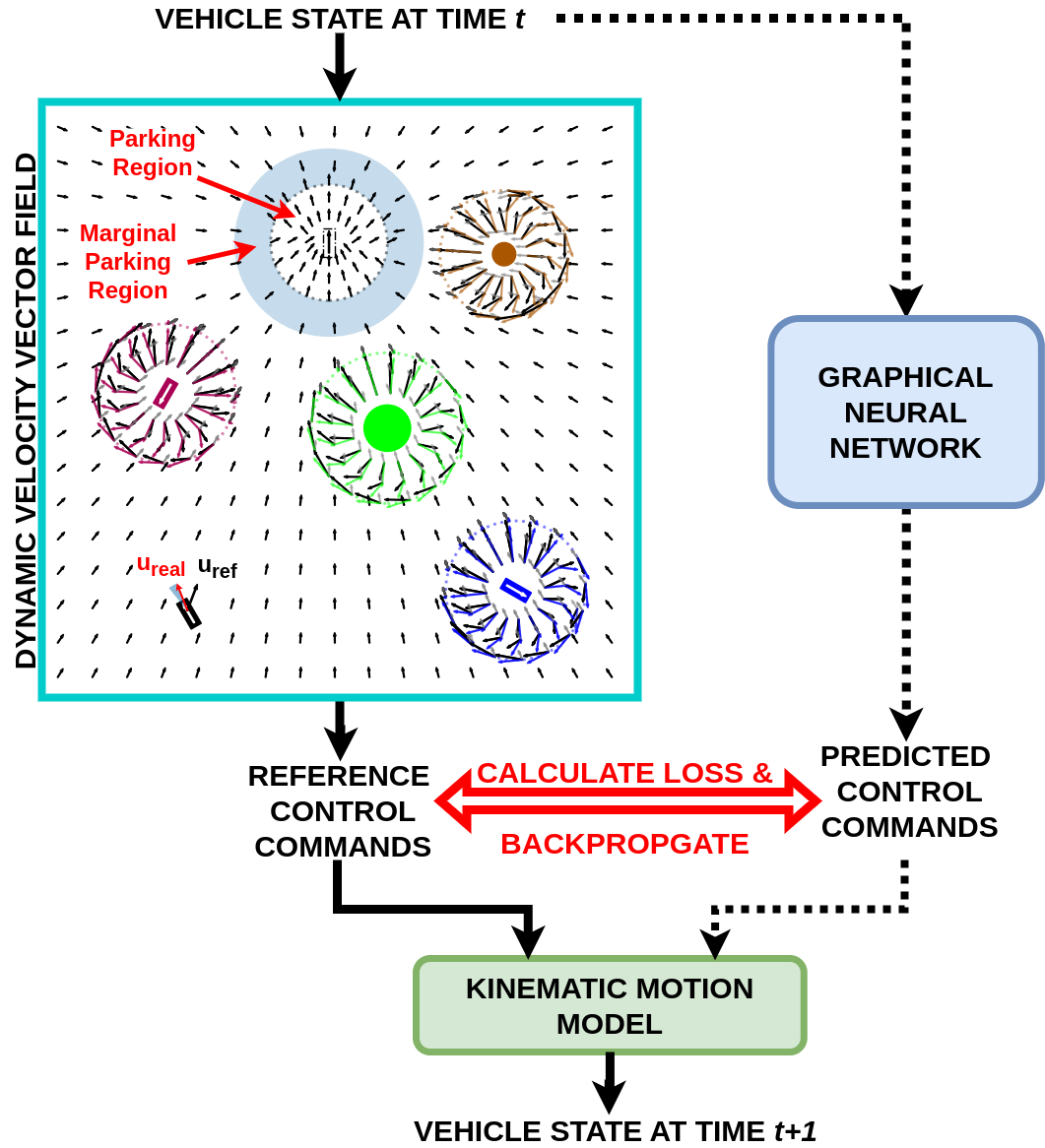
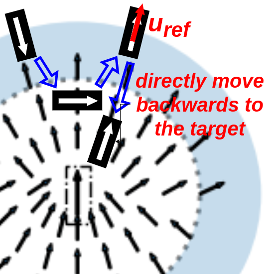
An example of the dynamic velocity vector field is shown in the project page: https://yininghase.github.io/MA-DV2F/#VD. Note that DV2F for the neighboring blue & maroon vehicles is likewise created separately (not shown here).
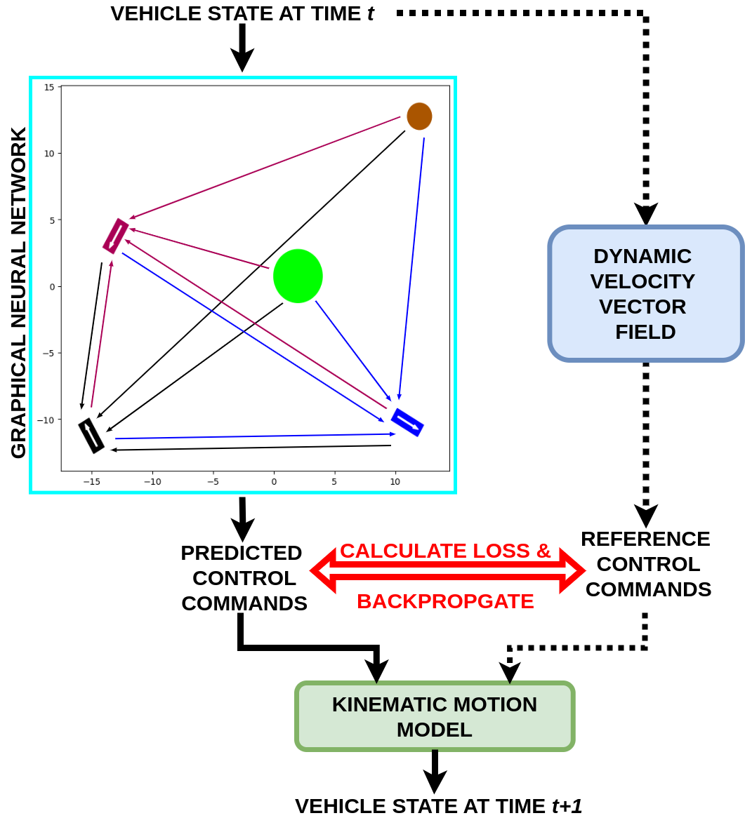
In this paper, we propose Multi-Agent Dynamic Velocity Vector Field (MA-DV2F), which generates vectors for the orientation and reference speed for every vehicle on the map. The vehicles then just need to follow in the direction of their respective velocity vector fields to successfully reach their destinations. The vector field for each vehicle is generated independently and can be adapted dynamically depending on the vehicle’s proximity to other agents (neighbouring vehicles or obstacles). Decoupling reduces the complexity of adding vehicles & allows for parallel generation of DV2F of each vehicle, thereby increasing the throughput. An added benefit of our approach is that the generated DV2F can be used to train a learning based graphical neural network (GNN) in a self-supervised manner. This self-supervised learning based approach neither requires tedious labeling of data nor necessitates sample inefficient environment exploration. We test our framework under challenging collision prone environments. A scenario is regarded to be challenging if trajectories of different vehicles considered independently from other agents intersect at multiple places at the same time. This would necessitate a collision avoidance maneuver for safe navigation towards the target.
Fig. 1 shows the pipeline for both the MA-DV2F (left branch, solid arrows) and optional training of the the self-supervised GNN counterpart (right branch, dotted arrows). The input is a continuous state representation of all the multiple vehicles and the outputs are the corresponding continuous control variables. The vehicles are non-holonomic with rotation radius determined by the kinematic model.
We summarize the contribution of this letter as follows:
-
•
Our proposed MA-DV2F outperforms other concurrent learning and search based approaches for the task of multi agent navigation in challenging, collision prone environments.
-
•
Even the self-supervised learning based counterpart of MA-DV2F scales better than other learning and search based methods.
-
•
MA-DV2F can determine the solutions orders of magnitude faster than other SOTA search based approaches.
-
•
We shall release the complete code of MA-DV2F upon acceptance on the project page here: https://yininghase.github.io/MA-DV2F/.
The project page also contains additional supplementary information such videos better depicting the operation of our method in comparison with other approaches, details of the challenging scenarios, dynamics of the velocity field at different regions on the navigation grid etc.
II Related Work
[16] proposed using Artificial Potential Fields (APF) for trajectory planning. An agent is subjected to an attractive potential force towards the target which serves as the sink and a repulsive potential force away from obstacles [17, 18]. However, a common problem with such methods is their propensity to get stuck in local minima [19, 20] when the attractive force from the target is cancelled out by the repulsive force arising from an another agent for e.g. when the ego-vehicle is symmetrically aligned with other agents to the target [21] and thus leading to a bottleneck situation. We break such bottlenecks by enforcing the vehicles to move in the clockwise direction.
[13] proposed a two level tree based search algorithm for multi-agent path finding. However, the tree may grow exponentially, making the search inefficient. This is because multi-agent path planning methods on trees and graphs are known to be NP-hard [22] since the search space grows exponentially as the number of agents rise [13]. Nevertheless, [14] used [13] to generate expert data for training a GNN model that can scale up to more vehicles than trained on. [23] uses RL and proposes a dense reward function to encourage environmental exploration. However, the need for exploration tends to make the learning sample-inefficient [24, 25] particularly when compared with imitation learning approaches [26]. [27] rather combines RL for single agent path planning with imitation learning to learn actions that can influence other agents. All approaches described above work either on a discrete grid, discrete action space, assume holomonic robots or their combination.
CL-MAPF [9] uses a Body Conflict Tree to describe agent collision scenarios as spatiotemporal constraints. It then applies a Hybrid-State A* Search algorithm to generate paths satisfying both kinematic and spatiotemporal constraints of the vehicles. However, under challenging test scenarios with vehicles crowding together, the algorithm takes long to search for a solution and can easily time out. To find feasible solution for large-scale multi-vehicle trajectory planning, CSDO [10] first searches for a coarse initial guess using a large search step. Then, the Decentralized Quadratic Programming is implemented to refine this guess for minor collisions. GCBF+ [8] based on GCBF [7] aims to provide safety guarantees utilizing control barrier functions (CBF). A Graphical Neural Network is trained to learn agent control policy.
III Framework
III-A Problem Description
We aim to solve the task of multi-agent navigation in unconstrained environments. Given dynamic vehicles and static obstacles in the scene, the task is to ensure each vehicle reaches its desired destination while avoiding collision with other agents. The state vector for ego-vehicle () at current time can be represented as , where and shows the position, , the orientation and the speed at current time . Meanwhile, and are co-ordinates of the target position, and is the target orientation. Each ego-vehicle is controlled by a control vector , where and are the pedal acceleration and steering angle, limited in magnitude by and respectively. The obstacle () is represented by a state vector , where and is the position, and is the radius of the circle circumscribing all vertices of the obstacle. The kinematics of the vehicles is modeled using the bicycle model [28].
| (1) |
It describes how the equations of motion can be updated in time increments of assuming no slip condition, valid under low or moderate vehicle speed when making turns. Note that and are the tuneable hyper-parameters modeling the environment friction and vehicle wheelbase respectively.
We create a velocity vector field for each vehicle, which in turn can dynamically generate reference control variables. Generation of the velocity field can be divided into two stages:
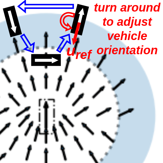
The orientation which a vehicle should possess at any position on the map is referred to as the Reference Orientation and is represented as a unit vector. The black arrows in Fig. 1 show the reference orientation for the black ego vehicle at different positions in the map. It can be seen that the arrows attract the ego-vehicle towards its target while repelling it away from the other vehicles and obstacles. Note that the current orientation of the ego-vehicle is not aligned with the reference orientation at its existing position. Therefore, we ought to find the control variables which align the ego-vehicle with the reference orientation. Apart from the reference orientation at each position in the map, the ego-vehicle also has a reference speed which should be attained by the control variables. Lastly, note that apart from the black vehicle, a separate reference orientation map is also created for the blue and red vehicles present in Fig. 1 (not shown in the Figure).
Hence, our task of multi-agent navigation simplifies to finding the reference orientation maps and corresponding reference speed for each vehicle independently. In the subsequent sub-section, we describe how the reference orientation and speed are estimated.
III-B Estimation of Reference Orientation
We first define some frequently used functions and vectors before we begin discussion of reference orientation estimation. The vector function is the function which takes a non-zero vector as input and divides by its magnitude to convert it into a unit vector.
Other scalar functions include and which both output 1 if the scalar input is positive. However, outputs -1, while outputs 0 when is negative. We now define the vector from the next position of ego vehicle to
-
•
its target position as
-
•
the position of the static obstacle as
-
•
next position of another vehicle as
The unit vector along the Z-axis is , while the unit orientation vector of the ego vehicle at the current target states are given by and respectively.
For the ego vehicle , the target reaching component of the reference orientation is defined as:
| (2) |
where is the parking threshold (black dotted circle in Fig. 1) and is the marginal parking threshold (shaded blue region in Fig. 1). is the default reference speed, estimation of which is explained in Subsection III-C. is the threshold above which an additional term is introduced when the vehicle is within the parking threshold.
Equation 2 shows that when the ego-vehicle is far away from the parking threshold, the reference orientation is in the direction of . However, as the ego-vehicle approaches the target and the velocity is high, then the vehicle might overshoot the target and enter the shaded marginal parking threshold region. In this case the direction of the orientation is flipped using . This is to prevent the vehicle from moving in circles. A detailed explanation of this is given in the supplementary file on the project page: https://yininghase.github.io/MA-DV2F/supplementary.pdf.
Equation 2 also shows for the condition when the distance falls below the parking threshold , and is closer to the target. The ego vehicle should be guided to not only reach the position of the target () but also be aligned with the target orientation (). The balancing act between these two conditions is handled by the term in Equation 2. Like previously, in makes sure the reference and target orientations are in the same directions when parking. The term in is designed to expedite the parking behavior when the vehicle position is exactly on the left or the right side of the target and the vehicle orientation is parallel to the target orientation.
Besides reaching the target, the ego vehicle should also avoid collision on its way to the target. This is realized by the collision avoiding component which comprises of collision avoidance between the ego vehicle and either static obstacle () or with another vehicle ().
The equation for determining () is given by:
| (3) |
where is the radius of the static object , is the radius of the smallest circle enclosing the ego-vehicles, is the static component, while is the speed-based dynamic safety margin for collision avoidance between ego vehicle and obstacle . Higher the vehicle speed , larger is this margin . When the distance between the ego vehicle and static object () is below the collision avoidance margin , then , and the reference orientation is modified to prevent collision with the static obstacle. Under this condition, the first term will guide the vehicle to drive away from the static obstacle. However, driving away is not enough as this might cause a bottleneck in cases where the obstacle is symmetrically collinear between the ego-vehicle and its target. We would additionally like the ego-vehicle to drive around the obstacle to reach the target for which the term is relevant. If the ego-vehicle is between the obstacle and target then (since ) and hence there is no need for the vehicle to drive around the obstacle. However, if that is not the case, then an additional component is added whose direction is given by and magnitude () is proportional to how far the vehicle is away from the obstacle. is given as the cross product between and with a zero being appended to the third dimension of which originally lies in the 2D space. The vector resulting from the cross-product is perpendicular to which causes the vehicles to move in the clockwise direction around the obstacle as shown in Fig. 2.
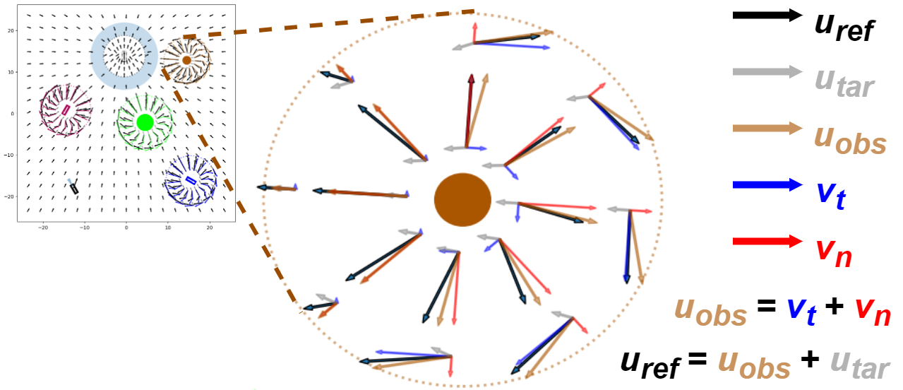
Likewise, the component for avoiding collision between the ego vehicle and another vehicle () is similar to Equation 3 except that the static obstacle radius will be replaced by the other vehicle’s radius in the term. Secondly, the speed based dynamic margin is rather than just .
The overall collision avoiding component is given by:
| (4) |
Finally, the ideal reference orientation vector ( in Fig. 1) is:
| (5) |
From this, the corresponding ideal reference orientation angle for ego vehicle can be calculated by applying to . However, kinematic constraints arising from the motion model (Equation 1) may prevent the vehicle from immediately attaining the ideal reference orientation in the next time step. Therefore, we instead use referred to as the real orientation. It is the reachable orientation closest to . The unit vector corresponding to this real reference orientation angle for ego vehicle is ( in Fig. 1) = .
III-C Estimation of Reference Speed
The reference speed is chosen after determination of the reference orientation, which depends on the situation the vehicle is in. Fig. 3(b) shows a scenario wherein a vehicle is at the same location next to an obstacle but with opposite orientations. This determines if the velocity should move the car forward or backward.
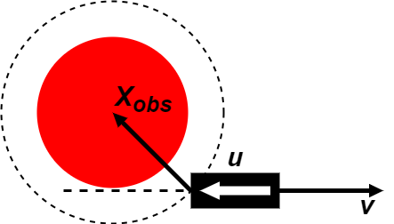
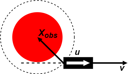
, the ego vehicle is facing the obstacle, i.e. , in which case the vehicle should be forbidden to move forwards. In Fig. 3(b), the ego vehicle is oriented away from the obstacle, i.e. , in which case the vehicle should be prevented from moving backward.
We use the logical or () and logical and () operators [29] to describe the criteria for collision avoidance between ego vehicle and static obstacle under such situations as:
| (6) |
where is same as defined in Equation 3, is the an additional tolerance for the collision checking region. equalling indicates the ego vehicle is forbidden to drive forwards towards obstacle . This happens when the angle between the reference orientation () and the vector from the ego vehicle to the obstacle () is less than i.e. . Likewise, equaling happens when indicating that the ego vehicle is forbidden to drive backwards.
Similarly for the case of ego vehicle and another vehicle , the conditions for preventing the ego-vehicle from moving forward or backward are the same as described in Equation 6 except that replaces .
Summarising the results above, the magnitude and sign of the velocity depends on the combination of these boolean variables i.e. , and as follows:
| (7) |
The first 3 conditions check whether or not there is a potential for collision. The velocity is , when the ego-vehicle is prevented from moving backwards () but allowed to move forward () and when vice versa. The reference velocity is zero when the ego-vehicle is prevented from moving either forward () or backward (). In all other cases, the velocity is defined as:
| (8) |
where and are the acceptable position and orientation tolerances for deciding to stop the vehicle at the target. When the ego vehicle is within the parking radius, it reduces its speed as it gets closer to the target position and orientation. This is achieved by the multiplier , which is proportional to when the vehicle state is very close to the target state and when farther away from the tolerance. The square root accelerates the vehicle approaching its target when there is still some distance between the current state and target state, i.e. . When the vehicle is already very close to the target state, i.e. (), the ratio prevents the vehicle from shaking forward and backward. For , the first term: , decreases linearly with the ego vehicle distance to its target, and the second term, i.e. , reduces linearly with the angle difference between the reference and target orientation angles. However, we do not allow the reference parking speed to be any higher than the default reference speed . So, is clipped to a maximum of . controls whether the ego vehicle moves forwards or backwards by checking . Originally, the vehicle should move forwards when facing the target, i.e. , and move backwards when backing toward the target, i.e. . However, to prevent the vehicle from changing direction at high frequency within short traveling distances, we set a margin allowing the vehicle to keep its previous direction when .
When the ego vehicle is out of the parking area of radius , the reference speed takes the forn , where the reference speed takes the default value , but changes to negative, i.e. , when .
The final ideal reference speed for ego vehicle is:
| (9) |
Similar to the reference orientation, the ideal reference speed may not achievable due to the limitation of the maximum pedal command. The real reference speed is therefore the reachable speed value closest to .
Calculation of Reference Steering Angle and Reference Pedal: Given the reference orientation and velocity, the Vehicle Kinematic Equation 1 can be inverted to determine the reference steering angle and pedal acceleration for controlling the vehicle at time :
| (10) |
These reference control commands can either be directly used to control the vehicles, or as labels for training the GNN model in a self-supervised manner using the architecture of [12].
IV EXPERIMENTS
IV-A Algorithm Evaluation
To assess the performance of our MA-DV2F approach and its learning based counterpart (self-supervised GNN model), we compare with other recent learning and search/optimization based algorithms in challenging, collision prone test cases. The recent learning based approaches include [12] which is a GNN model trained in a supervised manner and an extension of [7] i.e. GCBF+ [8], an RL-inspired GNN model incorporating safety constraints. Meanwhile, the two search/optimization based algorithms used for comparison include CL-MAPF [9] and CSDO [10]. The test dataset comprises of challenging, collision prone scenarios with the number of vehicles ranging from 10 to 50 and static obstacles chosen between 0 and 25. Note that, all the static obstacles in the test cases are fixed to be circles with fixed radius because of the limitation of the CL-MAPF and CSDO environment setting and because it circumscribes an obstacle of arbitrary shape, allowing for safer behaviour. For the GCBF+, we use the DubinsCar model because it has vehicle kinematics most similar to ours. As GCBF+ has a completely different working domain with different map and agent sizes, we scale our test cases when running GCBF+ under the rule that the ratio of the map size and the agent size remains equal across all the algorithms. Details regarding the generation of test samples are given in the supplementary file on the project page.
Table I shows the evaluation results of the different methods across the different vehicle-obstacle combinations described earlier against the success rate metric [8]. It measures the percentage of vehicles that successfully reach their targets within a tolerance without colliding with other objects along the way. The results show that our MA-DV2F outperforms other algorithms achieving almost 100% success rate across all vehicle-obstacle combinations. Even the self-supervised GNN model performs far better than other algorithms when scaling the number of vehicles. Only the CSDO algorithm has slightly better results than our GNN model when the number of agents are low (20). However, CSDO’s performance drops drastically as the number of agents are increased under these challenging conditions. Note that the GCBF+ pipeline only checks whether the agents reach their target positions but ignores the target orientations as shown in the project page: https://yininghase.github.io/MA-DV2F/#MC which explains why it has such poor performance. Therefore, we additionally evaluate GCBF+ by ignoring the orientation and only considering the position. Results of which are shown in the second last column. Even then, the GCBF+, does not match the performance of MA-DV2F.
| Number of | Number of | MA-DV2F | Self-Supervised | CSDO | CL-MAPF | GCBF+ | GCBF+ | Supervised |
|---|---|---|---|---|---|---|---|---|
| Vehicles | Obstacles | (Ours) | Model (Ours) | [10] | [9] | [8] | (only position) | Model [12] |
| success rate | ||||||||
| 10 | 0 | 1.0000 | 0.9929 | 0.9693 | 0.4290 | 0.0613 | 0.9021 | 0.7285 |
| 20 | 0 | 1.0000 | 0.9895 | 0.9400 | 0.4963 | 0.0563 | 0.8169 | 0.2041 |
| 30 | 0 | 1.0000 | 0.9793 | 0.8820 | 0.4977 | 0.0458 | 0.7550 | 0.0477 |
| 40 | 0 | 1.0000 | 0.9760 | 0.7063 | 0.5632 | 0.0451 | 0.7080 | 0.0137 |
| 50 | 0 | 1.0000 | 0.9686 | 0.6523 | 0.5992 | 0.0426 | 0.6618 | 0.0045 |
| 10 | 25 | 0.9952 | 0.9458 | 0.9682 | 0.5640 | 0.0509 | 0.7192 | 0.3734 |
| 20 | 25 | 0.9902 | 0.9208 | 0.9663 | 0.5997 | 0.0393 | 0.6479 | 0.0756 |
| 30 | 25 | 0.9844 | 0.8998 | 0.8456 | 0.6320 | 0.0385 | 0.5754 | 0.0196 |
| 40 | 25 | 0.9772 | 0.8723 | 0.6723 | 0.6531 | 0.0330 | 0.5211 | 0.0068 |
| 50 | 25 | 0.9704 | 0.8504 | 0.5897 | 0.6749 | 0.0290 | 0.4789 | 0.0028 |
IV-B Discussion
Investigating failure Causes: Note that the Success rate metric measures a model’s ability to not only reach its destination but also avoid collisions. Therefore, for challenging test cases, a navigation algorithm may fail due to two main reasons: the algorithms behave too aggressively by driving the vehicles to their targets albeit at the cost of colliding with other agents or behaves too conservatively to ensure safety of the vehicles resulting in some vehicles getting stuck mid-way without reaching their targets. Therefore to disambiguate between the two causes, we additionally evaluate all algorithms against the Reach rate and Safe rate metrics as proposed in [8]. Reach rate measures the percentage of vehicles that reach their targets within a tolerance disregarding any collisions along the way. Meanwhile, the Safe rate calculates the percentage of vehicles that do not collide with any other agents irrespective of whether or not they reach their targets. Fig. 4 shows the performance of the different methods against the Reach Rate and Safe Rate metrics. It can be seen that the supervised GNN model behaves rather aggressively reaching the target in majority of the cases albeit at the cost of multiple collisions leading to high Reach but low Safe rates. In contrast, CL-MAPF [9] takes a greedy strategy in its optimization/search pipeline. It can quickly find the path for some vehicles which are easy to plan. But then it is unable to find paths for other vehicles and gets stuck in this partial solution. This greedy strategy lead to a low reach rate, but high safe rate since no collisions happen among vehicles that do not move.
GCBF+ has a higher safe rate than reach rate. This is not because the vehicles fail to reach their target, but rather because they reach the target at an incorrect orientation. This is aligned with the intuition described in IV-A and is further corroborated by the fact that when orientation is ignored in the evaluation and only position is considered, the reach rate jumps drastically. Nevertheless, it is still much lower than both our MA-DV2F and its GNN self-supervised counterpart. They are the only 2 methods which maintain a consistent high performance against both metrics across all vehicle-obstacle combinations.
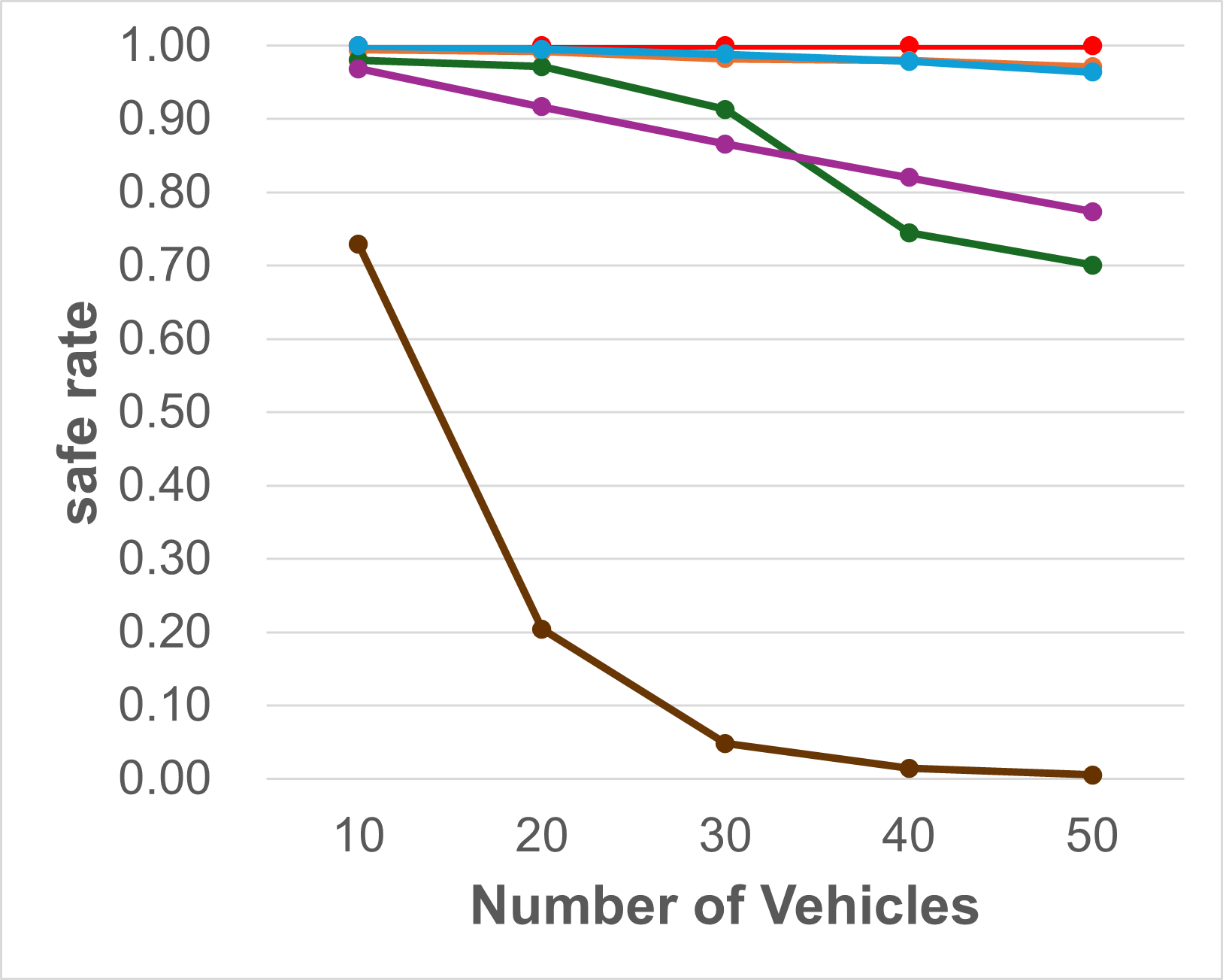
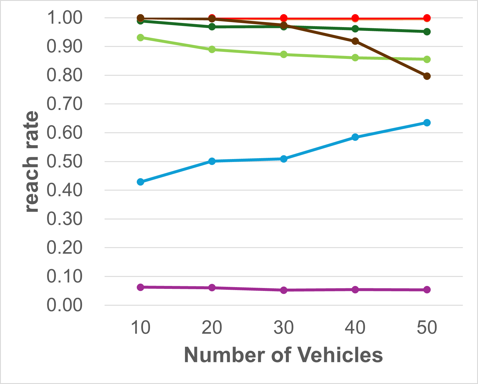
Preventing Bottlenecks: A common problem with other planning algorithms is that vehicles tend to crowd within a small sub-region in the map. This leads to these algorithms either unable to find an optimal path resulting in all vehicles becoming stationary at their place (low reach rate) or finding sub-optimal paths resulting in more collisions among vehicles (low safe rate). To prevent such bottlenecks in our MA-DV2F model, Equation 3 causes all the vehicles to drive in the clockwise direction when encountering other agents. This leads to a roundabout driving behavior which breaks the bottleneck and can be visualized on the project page: https://yininghase.github.io/MA-DV2F/#RE. Due to this, the vehicles are capable of eventually reaching their targets,by making a detour around the other agents, resulting in both a high Reach and Safe rate. Our trained GNN model also adapts this behaviour.
Intermediate Success Rate: One might wonder if the MA-DV2F method outperforms every other method, what is the advantage of its self-supervised GNN model counterpart? One reason is that MA-DV2F behaves conservatively in some simple test cases even though there is no collision risk nearby, causing the vehicles to take a longer time to finish the journey. This is because the speed is limited to . On the other hand, the self-supervised GNN counterpart is free from this restriction. If can move faster when it is far away from its target and there is less risk of collision with other objects. The figures in project page: https://yininghase.github.io/MA-DV2F/#ISR show the difference of the success rate between the self-supervised GNN model and MA-DV2F as a function of time. At the beginning when the vehicles tend to be far away from their targets, the GNN allows high velocity for vehicles, thereby causing some vehicles to reach their target faster leading to a success rate greater than that for MA-DV2F. This can also seen in the example in project page: https://yininghase.github.io/MA-DV2F/#MC, the vehicles by GNN can drive faster towards the targets than by MA-DV2F. However, maintaining a high velocity also leads to higher risk of collision when encountering challenging situations as time progresses and the success rate of MA-DV2F will gradually catch up and eventually exceed the GNN.
| Number of | Number of | MA-DV2F | CSDO | CL-MAPF |
| Vehicles | Obstacles | (Ours) | [10] | [9] |
| total runtime for 1000 test cases | ||||
| 10 | 0 | 4.152 | 195.919 | 125643.851 |
| 20 | 0 | 5.848 | 1044.360 | 219251.537 |
| 30 | 0 | 7.885 | 6179.536 | 328471.949 |
| 40 | 0 | 8.492 | 12342.014 | 376417.421 |
| 50 | 0 | 10.512 | 18306.779 | 395962.103 |
| 10 | 25 | 10.322 | 352.096 | 89838.921 |
| 20 | 25 | 12.260 | 2213.838 | 163001.473 |
| 30 | 25 | 13.733 | 9148.955 | 190907.288 |
| 40 | 25 | 15.562 | 14350.735 | 224962.016 |
| 50 | 25 | 18.405 | 16598.068 | 253495.187 |
Runtime Analysis: We compare the runtime of MA-DV2F with concurrent search based methods (CSDO and CL-MAPF). TABLE II shows the total runtime of all the 1000 test cases for each vehicle-obstalce combinations. All methods were evaluated on a machine with an Intel Core i7-10750H CPU and GeForce RTX 2070 GPU. As can be seen, our MA-DV2F, is orders of magnitude faster than its peers, since it has the ability to run the different scenarios within a batch in parallel. Meanwhile CSDO and CL-MAPF are search/optimization-based algorithms that need to solve each test cases one-by-one. Note that CL-MAPF would continue its search until a solution is found, which is why the maximum allowed runtime needs to be clipped, otherwise the runtime would be even larger. Note that the evaluations in the experiments were done for only upto 50 vehicles, since other algorithms are either extremely slow or have drastically reduced performance when scaling. However, our method is capable of scaling to a far greater number of vehicles than just 50 as can be observed on the project page for scenarios with 100, 125, 250 vehicle-obstacle combinations: https://yininghase.github.io/MA-DV2F/#LE.
Lastly, note that the runtime analysis is not done for the learning based methods since, it is dependent on the GPU rather than the algorithm itself. Therefore, for the same model architecture, the runtime will be the same for all learning based algorithms.
Limitations: If the vehicles are densely packed or their targets are within the safety margins of one another, then due to their non-holonomic behavior there might not be enough space for them to navigate without risking a collision. In such a scenario, the vehicles will act conservatively and hesitate to proceed so as to avoid collisions leading to less vehicles reaching the target. A similar outcome is observed, if some vehicles start behaving unexpectedly, wherein the safety margin would need to be increased to mitigate the risk of collision, albeit at the expense of reaching the target. More details on sensitivity analysis of the effect of change in static component of the safety margin () and visualization of the limitations is in the supplementary file and the project page.
V Conclusion
This work introduced MA-DV2F, an efficient algorithm for multi-vehicle navigation using dynamic velocity vector fields. Experimental results showed that our approach seamlessly scales with the number of vehicles. When compared with other concurrent learning and search based methods, MA-DV2F has higher success rate, lower collision metrics and higher computational efficiency.
Acknowledgements: We thank Ang Li for the discussions and his feedback on the setup of the experiments.
References
- [1] X. Cao, M. Li, Y. Tao, and P. Lu, “Hma-sar: Multi-agent search and rescue for unknown located dynamic targets in completely unknown environments,” IEEE Robotics and Automation Letters, 2024.
- [2] L. Bartolomei, L. Teixeira, and M. Chli, “Fast multi-uav decentralized exploration of forests,” IEEE Robotics and Automation Letters, 2023.
- [3] F. Kudo and K. Cai, “A tsp-based online algorithm for multi-task multi-agent pickup and delivery,” IEEE Robotics and Automation Letters, 2023.
- [4] B. Li and H. Ma, “Double-deck multi-agent pickup and delivery: Multi-robot rearrangement in large-scale warehouses,” IEEE Robotics and Automation Letters, 2023.
- [5] D. Zhu, Q. Khan, and D. Cremers, “Multi-vehicle trajectory prediction and control at intersections using state and intention information,” Neurocomputing, p. 127220, 2024.
- [6] B. Nebel, “On the computational complexity of multi-agent pathfinding on directed graphs,” in Proceedings of the International Conference on Automated Planning and Scheduling, 2020.
- [7] S. Zhang, K. Garg, and C. Fan, “Neural graph control barrier functions guided distributed collision-avoidance multi-agent control,” in Conference on Robot Learning. PMLR, 2023, pp. 2373–2392.
- [8] S. Zhang, O. So, K. Garg, and C. Fan, “Gcbf+: A neural graph control barrier function framework for distributed safe multi-agent control,” IEEE Transactions on Robotics, pp. 1–20, 2025.
- [9] L. Wen, Y. Liu, and H. Li, “Cl-mapf: Multi-agent path finding for car-like robots with kinematic and spatiotemporal constraints,” Robotics and Autonomous Systems, 2022.
- [10] Y. Yang, S. Xu, X. Yan, J. Jiang, J. Wang, and H. Huang, “Csdo: Enhancing efficiency and success in large-scale multi-vehicle trajectory planning,” IEEE Robotics and Automation Letters, 2024.
- [11] R. S. Sutton, “Reinforcement learning: An introduction,” A Bradford Book, 2018.
- [12] Y. Ma, Q. Khan, and D. Cremers, “Multi agent navigation in unconstrained environments using a centralized attention based graphical neural network controller,” in IEEE 26th International Conference on Intelligent Transportation Systems, 2023.
- [13] G. Sharon et al., “Conflict-based search for optimal multi-agent pathfinding,” Artificial intelligence, 2015.
- [14] Q. Li, F. Gama, A. Ribeiro, and A. Prorok, “Graph neural networks for decentralized multi-robot path planning,” in IEEE/RSJ international conference on intelligent robots and systems (IROS), 2020.
- [15] Y. Ma, A. Li, Q. Khan, and D. Cremers, “Enhancing the performance of multi-vehicle navigation in unstructured environments using hard sample mining,” arXiv preprint arXiv:2409.05119, 2024.
- [16] O. Khatib, “Real-time obstacle avoidance for manipulators and mobile robots,” in Proceedings. 1985 IEEE international conference on robotics and automation, vol. 2. IEEE, 1985, pp. 500–505.
- [17] M. Reda, A. Onsy, A. Y. Haikal, and A. Ghanbari, “Path planning algorithms in the autonomous driving system: A comprehensive review,” Robotics and Autonomous Systems, vol. 174, p. 104630, 2024.
- [18] A. Loganathan and N. S. Ahmad, “A systematic review on recent advances in autonomous mobile robot navigation,” Engineering Science and Technology, an International Journal, vol. 40, p. 101343, 2023.
- [19] Á. Madridano, A. Al-Kaff, D. Martín, and A. De La Escalera, “Trajectory planning for multi-robot systems: Methods and applications,” Expert Systems with Applications, vol. 173, p. 114660, 2021.
- [20] J. Hou, G. Chen, J. Huang, Y. Qiao, L. Xiong, F. Wen, A. Knoll, and C. Jiang, “Large-scale vehicle platooning: Advances and challenges in scheduling and planning techniques,” Engineering, 2023.
- [21] I. Iswanto et al., “Artificial potential field algorithm implementation for quadrotor path planning,” International Journal of Advanced Computer Science and Applications, 2019.
- [22] J. Yu and S. LaValle, “Structure and intractability of optimal multi-robot path planning on graphs,” in Proceedings of the AAAI Conference on Artificial Intelligence, vol. 27, no. 1, 2013, pp. 1443–1449.
- [23] H.-T. Wai, Z. Yang, Z. Wang, and M. Hong, “Multi-agent reinforcement learning via double averaging primal-dual optimization,” Advances in Neural Information Processing Systems, vol. 31, 2018.
- [24] D. Li, D. Zhao, Q. Zhang, and Y. Chen, “Reinforcement learning and deep learning based lateral control for autonomous driving [application notes],” IEEE Computational Intelligence Magazine, 2019.
- [25] N. Vithayathil Varghese and Q. H. Mahmoud, “A survey of multi-task deep reinforcement learning,” Electronics, vol. 9, no. 9, 2020.
- [26] A. Dosovitskiy, G. Ros, F. Codevilla, A. Lopez, and V. Koltun, “CARLA: An open urban driving simulator,” in Proceedings of the 1st Annual Conference on Robot Learning, 2017.
- [27] G. Sartoretti, J. Kerr, Y. Shi, G. Wagner, T. K. S. Kumar, S. Koenig, and H. Choset, “Primal: Pathfinding via reinforcement and imitation multi-agent learning,” IEEE Robotics and Automation Letters, 2019.
- [28] D. Wang and F. Qi, “Trajectory planning for a four-wheel-steering vehicle,” in IEEE International Conference on Robotics and Automation, 2001.
- [29] M. M. Mano, Digital logic and computer design. Pearson Education India, 2017.
VI Supplementary
VI-A Further Explanation of MA-DV2F
In this Subsection, we further elaborate some the design choices for Equation 2 used to determine the reference orientation. The Equation is repeated here again for clarity:
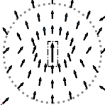
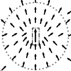
Circular Motion Prevention: Equation 2 shows that when the ego-vehicle is far away from the parking threshold, the reference orientation is in the direction of . However, as the ego-vehicle approaches the target and the velocity is high, then the vehicle might overshoot the target and enter the shaded marginal parking threshold region causing the current ego-vehicle orientation to be opposite to as seen in Fig. 5(a). This will make the vehicle go in circles in an attempt to align itself with the reference orientation. A better alternative would be switch the reference orientation direction so that it is aligned with the ego-vehicle orientation and drive the car in reverse as shown in Fig. 5(b). This is done by dynamically switching the reference orientation depending on the sign of the dot product: .
Parking behaviour Refinement: In Equation 2, an additional term: was introduced in to refine the parking behavior when the vehicle position is exactly on either the left or the right side of the target. As can be seen in Fig. 6, this additional refinement term causes the reference orientation to be more biased towards the target position within the parking region. The ego vehicle aligns itself better to the reference orientation there, while simultaneously allowing it to reach the final target quicker. Removing this term would make the reference orientations rather parallel to the final target causing the ego vehicle to oscillate forward and backwards around the target leading to a longer parking time. This is particularly true when the ego vehicle position is exactly to the left or to the right side of the target.
VI-B Self-supervised Training of GNN Model
The reference steering angles and reference pedal acceleration mentioned in Section III cannot only be used to control the vehicles directly, but also as labels to supervise training of the GNN model. This approach can therefore additionally be used to train a learning based Graphical Neural Network (GNN) controller in a self-supervised manner using these control labels and network architecture given in [12]. However, [12] requires running an optimization based procedure offline to collect enough training data with ground truth labels. This is a computationally expensive and slow process when the number of agents are large. In contrast, our self-supervised learning method is capable of directly training the model online during the simulation process without collecting ground truth labels beforehand. Note that in [12], all the vehicle nodes in the GNN model will have incoming edges from any other vehicle or obstacle nodes. In this case, the number of edges in the graph will grow quadratic to the number of agents(neighbouring vehicles/obstacles), leading to a heavy computational burden when when scaling to more agents. Thus, we remove edges between the neighboring agent or and the ego vehicle if the distance between them is greater than the threshold given by:
| (11) |
Training Pipeline: The self-supervised learning pipeline is shown in Fig. 7. At the start of training, different training samples with multiple agents placed at random positions are generated as the start points of the DV2F simulations. Each sample only contains the states of the vehicles and static obstacles without any control labels. At each step during the simulation, the reference control variables of each vehicle is determined online using the DV2F according to the states of the vehicles and obstacles at that time. The loss is calculated on the fly based on the reference control variables and the predicted control variables by the model. This loss is then back-propagated to update the model immediately at the current step. Unlike [12] which solves the individual optimization problem for each case one-by-one, our dynamic velocity vector field determines reference control variables in a closed-form solution. Thus, we can run one simulation with multiple cases as a batch running in parallel, and then change to another batch for the next turn of simulation until finishing all the training cases as an epoch.
Loss Function: The dynamic velocity vector field gives a low reference speed limited by . However, if the vehicle is still far away from its target and has low risk to colliding with other agents, the speed limit of can be removed allowing the vehicle to move faster to its target. To this end, we first define a vehicle state cost to evaluate vehicle control. Assume the current vehicle position , orientation and speed are fixed, for the given vehicle control variables and , we first apply the vehicle kinematic equation to obtain , , and . We redefine , and for the time . The vehicle state cost is then calculated as follows:
| (12) |
where and are defined same as in Equation 3 mentioned in Section III-B, measures the distance of the ego vehicle to its target, and and evaluate the collision risk of the ego vehicle. The gradient of this vehicle state cost should alone be enough to guide the GNN model in learning to reach the target while avoiding collisions. However, in practice, the GNN does not converge to the optimal due to high non-linearities in Equation 12. Therefore, we combine this equation with the labels obtained from the dynamic velocity vector field which expedites the model training.
The overall loss function used in this pipeline is defined as follows:
| (13) |
where the , and are the reference steering angle, reference pedal and calculated reference speed from dynamic velocity vector field, the , and are the corresponding values predicted by the GNN model. During training, the steering angle is fully supervised by reference steering angle . However, the pedal acceleration loss comprises one of two parts depending on the condition of the vehicle. If the vehicle is far way from the parking region, i.e. , and the default reference speed limits the predicted speed, i.e. , then the pedal loss is supervised by the relative vehicle state cost . This allows the vehicle to speed up when no other agents are nearby and slow down when getting close to other objects or its target. Otherwise, the pedal acceleration loss is supervised by the reference pedal . Note that we use the reference steering angle rather than the predicted steering angle to calculate the vehicle state cost.
VI-C Training & Test Data Generation
The advantage of our self-supervised approach is that the data for training the GNN model can be generated on the fly, since it does not require supervised labels. However, for the purpose of reproducibilty of our experiments, we generate data beforehand. One common option is to generate the samples by choosing a vehicle’s starting and target positions randomly on the navigation grid. However, the risk with this approach is that the dataset might be heavily skewed in favour of one scenario and may not capture other types of situations that the vehicle is expected to encounter. In contrast, our training regime is developed to handle these diverse situations. These situations can primarily be segregated into 3 modes: collision, parking and normal driving. In the collision mode, the vehicles are placed such that they have a high probability of collision. This is done by first randomly choosing a point on the grid, defined as a ”collision center”. The starting and target position of at least two vehicles are placed on opposite sides of this collision center with slight random deviation. Hence, the model will be pushed to learn a collision avoidance maneuver. Meanwhile, in the parking mode, the target position for each vehicle is sampled near its start position (within a distance of m). Note that in both the collision and parking modes, the position of the vehicles are also chosen randomly but with certain constraints i.e. starting and target positions being on the opposite sides of collision center (collision mode) or in close proximity (parking mode). In the normal driving mode, the starting and target positions are chosen randomly without any of the constraints described earlier. Lastly, for all modes the following additional conditions are to be fulfilled: No two target or two staring positions of vehicles can overlap. Likewise, if there are static obstacles, the starting/target positions cannot overlap with it. The starting position can be placed within an obstacle’s circle of influence but not a target position, since then the vehicle will struggle attaining equilibrium. The target position will attract the ego-vehicle whereas the obstacle influence will repel it. Our training dataset contains training cases from 1 vehicle 0 obstacles to 5 vehicles 8 obstacles, each with 3000 samples that in turn contains 1000 samples from each of the 3 modes. Each of these 3000 scenarios serve as the starting point for the simulation that is run for timesteps during training, in order for the vehicles to reach their target positions. As mentioned in Section IV-A, we also generate test scenarios range from 10 vehicles - 0 obstacles to 50 vehicles - 25 obstacles, each with 1000 samples. However, our test dataset is generated only using the collision mode.
Multiple training samples can be grouped as a batch and run simultaneously. However, this training simulation will always end with all the vehicles in the training batch approaching their targets and parking. To prevent the model from overfitting on parking behavior, we adopt a asynchronous simulation during the training. Specifically, a training batch if further divided into multiple mini-batches. These mini-batches are in different simulation time steps. In this case, within a training batch, there are always some training samples just starting, some driving the vehicles on the way and the rest parking the vehicles. Besides, for each time step during the training simulation, we also perturbs the vehicle state using a zero-mean Gaussian noise as a data augmentation. The standard variance decreases linearly along the simulation time : . The validation dataset reuse the training samples without random perturbation. The simulation length during validation is reduced to .
To train the neural network, we use the Adam optimizer with an initial learning rate of and weight decay of . The learning rate is reduced by factor of from its previous value, if the validation loss does not reduce for 15 epochs. The number of training epochs is set to be but training is prematurely stopped, if there is no decrease in the validation loss for epochs.
VI-D Experimental Settings
In this section, we elaborate the detailed hyper-parameter settings in our experiments.
In the vehicle kinematic Equation 1, the inverse of the vehicle length is and the friction coefficient is . The pedal acceleration threshold introduced in Section III-A is m/. The steering angle limits is radians. The timestep is s.
For the setting of velocity vector field in Subsection III-B and III-C, the default velocity is m/s. The parking threshold is m. The radius of the obstacle is sampled from m to m. The radius of the vehicle is fixed to be m. The and in the dynamic part of collision avoidance margin are determined to be the corresponding vehicle speed and the vehicle speed will not exceed the default velocity m/s in our MA-DV2F algorithm. The static part of collision avoidance margin is fixed to be m. The position tolerance and the orientation tolerance are m and m, respectively. The sensing radius of each vehicle should be large than the threshold determined in Equation 11.
VI-E Sensitivity Analysis
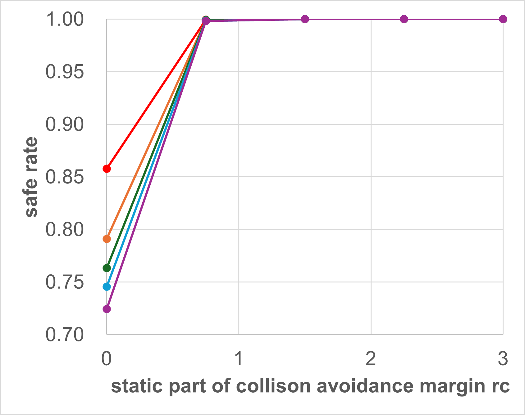
In this Subsection, we investigate how the collision avoidance margin influences the success rate. As the dynamic part of collision avoidance margin is determined by vehicle speed, we only change the static part in our experiment. As can be seen in Table III and Fig. 8, that if the safety margin rc is reduced from its default value of 1.5 m, the success rate reduces drastically. This is because MA-DV2F considers only those neighboring agents (other vehicles and obstacles) that are in its immediate vicinity. Hence, when determining steering commands for the ego-vehicle, MA-DV2F would not consider the presence of those agents that are close but not in the immediate vicinity. Therefore, if the ego-vehicle is moving at high speed, then by the time a neighboring vehicle enters its immediate vicinity, it might have been too late for the ego-vehicle to execute an evasive maneuver away from that neighboring vehicle. This will lead to higher probability of collision, hence a lower safe rate (Bottom row) and consequently a lower success rate (Top row) as can be seen in the plots in Fig. (a), for all the vehicle configurations (10-50 vehicles).
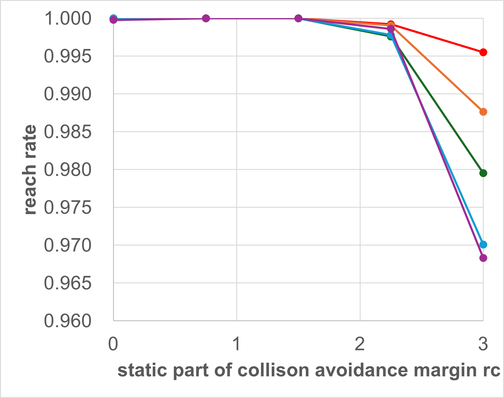
Conversely, if the safety margin rc is increased from its default value of 1.5 m, the success rate also reduces but for a different reason. Note that with a greater safety margin, the number of neighboring agents that would be considered by the MA-DV2F for steering command prediction will also be greater. This will cause the ego-vehicle to behave conservatively in order to prevent collisions at the expense of reaching the target. This results in a lower reach rate (center row) and consequentially a lower success rate (Top row). This is further exacerbated when there are obstacles in the scene (Right column), since the presence of obstacles reduces the region in which the vehicles can navigate without causing collisions.
| Number of | Number of | static part of collision avoidance margin | ||||
|---|---|---|---|---|---|---|
| Vehicles | Obstacles | 0.0 | 0.75 | 1.5 | 2.25 | 3.0 |
| success rate | ||||||
| 10 | 0 | 0.8576 | 0.9994 | 1.0000 | 0.9992 | 0.9955 |
| 20 | 0 | 0.7910 | 0.9990 | 1.0000 | 0.9991 | 0.9876 |
| 30 | 0 | 0.7631 | 0.9992 | 1.0000 | 0.9976 | 0.9795 |
| 40 | 0 | 0.7456 | 0.9984 | 1.0000 | 0.9978 | 0.9701 |
| 50 | 0 | 0.7244 | 0.9982 | 1.0000 | 0.9986 | 0.9683 |
| 10 | 25 | 0.5324 | 0.8363 | 0.9952 | 0.9577 | 0.6637 |
| 20 | 25 | 0.4146 | 0.7764 | 0.9902 | 0.9171 | 0.5375 |
| 30 | 25 | 0.3434 | 0.7339 | 0.9844 | 0.8713 | 0.4750 |
| 40 | 25 | 0.3032 | 0.7032 | 0.9772 | 0.8306 | 0.4480 |
| 50 | 25 | 0.2775 | 0.6843 | 0.9704 | 0.7945 | 0.4363 |