Machine learning potentials for complex aqueous systems made simple
Abstract
Simulation techniques based on accurate and efficient representations of potential energy surfaces are urgently needed for the understanding of complex aqueous systems such as solid-liquid interfaces. Here, we present a machine learning framework that enables the efficient development and validation of models for complex aqueous systems. Instead of trying to deliver a globally-optimal machine learning potential, we propose to develop models applicable to specific thermodynamic state points in a simple and user-friendly process. After an initial ab initio simulation, a machine learning potential is constructed with minimum human effort through a data-driven active learning protocol. Such models can afterwards be applied in exhaustive simulations to provide reliable answers for the scientific question at hand, or systematically explore the thermal performance of ab initio methods. We showcase this methodology on a diverse set of aqueous systems comprising bulk water with different ions in solution, water on a titanium dioxide surface, as well as water confined in nanotubes and between molybdenum disulfide sheets. Highlighting the accuracy of our approach with respect to the underlying ab initio reference, the resulting models are evaluated in detail with an automated validation protocol that includes structural and dynamical properties and the precision of the force prediction of the models. Finally, we demonstrate the capabilities of our approach for the description of water on the rutile titanium dioxide (110) surface to analyze the structure and mobility of water on this surface. Such machine learning models provide a straightforward and uncomplicated but accurate extension of simulation time and length scales for complex systems.
There is a great need for a better understanding of complex aqueous systems, in particular those involving solid-liquid interfaces, to promote progress in fields as diverse as heterogeneous catalysis, material design, biotechnology, and energy conversion or storage Zaera2012/10.1021/cr2002068; Bjorneholm2016/10.1021/acs.chemrev.6b00045. For this purpose, atomistic insight provided by computational approaches is urgently required, but off-the-shelf simulation techniques come with important limitations. Ab initio based methods, such as ab initio molecular dynamics (AIMD), struggle in terms of the accessible time and length scales, while traditional force field approaches are complicated to develop and often not accurate enough to provide reliable answers for complex interface problems. In recent years, machine learning potentials (MLPs) have become a promising alternative, bypassing expensive ab initio calculations and extending length and time scales in molecular simulations Behler2016/10.1063/1.4966192; Butler2018/10.1038/s41586-018-0337-2; Deringer2019/10.1002/adma.201902765; Kang2020/10.1021/acs.accounts.0c00472; Behler2021/10.1021/acs.chemrev.0c00868. This is exemplified in studies on the understanding of the unique properties of water Morawietz2016/10.1073/pnas.1602375113; Cheng2019/10.1073/pnas.1815117116; Gartner2020/10.1073/pnas.2015440117, structural and electronic transitions in disordered silicon Deringer2021/10.1038/s41586-020-03072-z, and phase transitions of hybrid perovskites Jinnouchi2019/10.1103/PhysRevLett.122.225701 to name but a few. The success of MLPs is grounded in a number of distinct approaches that have been introduced over the years, notably using artificial neural networks Behler2007/10.1103/PhysRevLett.98.146401; Ghasemi2015/10.1103/PhysRevB.92.045131; Schuett2017/10.1038/ncomms13890; Zhang2018/10.1103/PhysRevLett.120.143001; Unke2019/10.1021/acs.jctc.9b00181, or kernel based methods Bartok2010/10.1103/PhysRevLett.104.136403; Rupp2012/10.1103/PhysRevLett.108.058301; Thompson2015/10.1016/j.jcp.2014.12.018; Shapeev2015/10.1137/15M1054183; Li2015/10.1103/PhysRevLett.114.096405; Chmiela2017/10.1126/sciadv.1603015.
Despite compelling advances towards data-driven and automated techniques mostly in the context of active learning Gastegger2017/10.1039/c7sc02267k; Podryabinkin2017/10.1016/j.commatsci.2017.08.031; Zhang2019/10.1103/PhysRevMaterials.3.023804; Smith2018/10.1063/1.5023802; Deringer2018/10.1103/PhysRevLett.120.156001; Schutt2018/10.1063/1.5019779; Musil2018/10.1039/c7sc04665k; Schran2020/10.1021/acs.jctc.9b00805, the construction of a successful model, in particular for complex systems, remains a difficult task. This becomes most apparent when trying to achieve a high degree of transferability or generality, as for example recently shown in the development of general purpose MLPs for silicon Bartok2018/10.1103/PhysRevX.8.041048, carbon Rowe2020/10.1063/5.0005084, or phosphorous Deringer2020/10.1038/s41467-020-19168-z. The examples cited and many similar ones reported in the literature can take years to develop as broad regions of phase space have to be sampled by an appropriate balance of training points to provide reliable predictions across the board. As a consequence relatively few studies exist in which complex solid-liquid systems have been described with MLPs Natarajan2016/10.1039/c6cp05711j; Hellstrom2019/10.1039/c8sc03033b; Andrade2020/10.1039/c9sc05116c; Ghorbanfekr2020/10.1021/acs.jpclett.0c01739; Artrith2019/10.1088/2515-7655/ab2060. These limitations have hampered progress in understanding solid-liquid interfaces, where accurate MLPs are urgently needed and offer many opportunities for deepening our understanding of processes like wetting, ice formation, or liquid flow and friction under confinement.
However, the high degree of generality that most MLPs try to achieve is in practice not always needed to answer the scientific question at hand. Often, it is sufficient to sample just a small region of configuration space under specific thermodynamic and boundary conditions, while reaching the time and length scales at appropriate ab initio accuracy represents the true challenge. This is the main motivation behind the very promising on-the-fly learning techniques Li2015/10.1103/PhysRevLett.114.096405; Jinnouchi2020/10.1021/acs.jpclett.0c01061; Vandermause2020/10.1038/s41524-020-0283-z, (or surrogate models for global structure optimizations Bisbo2020/10.1103/PhysRevLett.124.086102) that do not aim for a high degree of generality. Yet, even these approaches have so far not had wide uptake for complex interfaces and they have been developed and validated on a system specific case by case basis.
Here, we present another approach to generate MLPs in a simple and fast fashion that is particularly suited for complex systems. To achieve this task, we make use of a 1) widely applicable, robust and scalable machine learning model for the representation of the structure-energy relation, 2) a general strategy for the generation and selection of representative training data, and finally 3) a comprehensive and automated validation procedure. By design we concentrate the development on a specific thermodynamic condition. This inherent loss of generality is counter-balanced by the speed of the development as well as the local (as opposed to global) accuracy of the MLP. The workflow to develop and apply such models follows broadly the following simple and computationally inexpensive steps. The relevant thermodynamic condition is initially sampled with a small-scale reference ab initio simulation. This trajectory is screened by a data-driven and automated active learning procedure to construct the machine learning model. The resulting model is then validated through a automated validation protocol and afterwards applied in large-scale simulations to answer the relevant scientific question. We show how these models can be developed with minimum human effort, while retaining reliable predictions over long time scales for complex aqueous systems at orders of magnitude lower computational cost than the original ab initio method. This methodology is applied to six exemplary aqueous systems, comprising the fluoride and sulfate ions in aqueous solution, water in carbon and hexagonal boron nitride nanotubes, water on a titanium dioxide surface, and water under molybdenum disulfide confinement.
Due to the efficient nature of this approach, both from a computational but also user perspective, such readily developed models can afterwards be applied in extensive molecular simulations to evaluate properties of interest. We demonstrate this in the present case for the description of water on the rutile titanium dioxide surface, for which we investigate structural and dynamical properties with extended molecular dynamics simulations. We believe that the change of paradigm of generating a machine learning model in a “cheap and simple” process as described here will lead to an increase in the adoption of MLPs to simulate complex systems. These concepts are also expected to be transferable to other machine learning approaches that can be easily coupled to the open-source active learning package, that we make freely accessible. Having shown that this approach is able to correctly capture the properties of various aqueous systems under confinement and at interfaces, we suggest that it outlines a straightforward strategy for the uncomplicated but accurate investigation of many technologically relevant systems.
Rapid development of committee neural network potentials
The implementation of our MLP framework relies on committee neural network potentials (C-NNPs) Schran2020/10.1063/5.0016004, in our case built from Behler-Parrinello NNPs Behler2007/10.1103/PhysRevLett.98.146401; Behler2017/10.1002/anie.201703114. While these models only consider the local environment of each atom explicitly within a finite range, long-range contributions can in principle be incorporated in MLPs as demonstrated in the literature Artrith2011/10.1103/PhysRevB.83.153101; Grisafi2019/10.1063/1.5128375; Ko2021/10.1038/s41467-020-20427-2; Yue2021/10.1063/5.0031215. The main idea behind the current approach is the combination of multiple NNPs in a “committee model”, where the committee members are separately trained from independent random initial conditions to a subset of the total training set. The resulting committee model has multiple benefits over its individual members. While the committee average, which is used as the prediction of the whole model, has been shown to provide better performance than the individual NNPs, the committee disagreement, which is defined as the standard deviation between the committee member predictions, grants access to an estimate of the error of the model. If scaled by a constant obtained by comparison to the true validation error Imbalzano2021/10.1063/5.0036522, the committee disagreement provides an objective measure of the accuracy of the underlying model. To construct a training set of such a model in an automated and data-driven way, new configurations with the highest disagreement can be added to the training set. This is an active learning strategy called query by committee and can be used to systematically improve a machine learning model, while making efficient use of the limited data available which provides an important advantage for the current application. Further details on the C-NNP methodology can be found in Ref. Schran2020/10.1063/5.0016004.
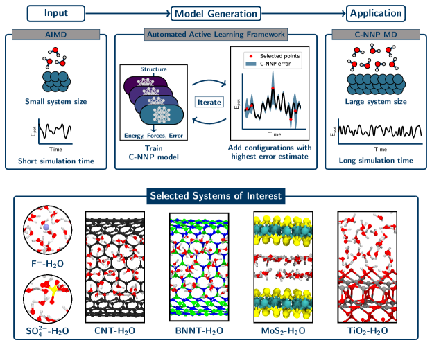
These concepts can be used for the rapid development of MLPs as described in the following and schematically depicted in the top panel of Fig. 1. Initially, a small-scale reference AIMD simulation is performed to sample the system of interest under the selected thermodynamic condition. Small-scale refers here mostly to the envisaged time and length scales of the final application, while they might still be considered large from the ab initio perspective. In practice, AIMD trajectories with a length of 30 ps have been sufficient for this purpose with system sizes that are large enough to cover all required local chemical environments. Given this trajectory, which can also come from existing previous work, we then construct the training set of the C-NNP model by selecting the most representative configurations for the system and condition of interest in an iterative active learning procedure. In the beginning, a small set of 20 structures is randomly selected from the reference trajectory in order to train an initial C-NNP model. Next, query by committee is used to actively select 20 configurations based on the highest committee disagreement in the atomic forces from the set of candidate structures provided by the reference trajectory. These points are added to the training set and an improved C-NNP model is trained to the extended training set. No additional ab initio reference calculations are required in this process, as the potential energy and atomic forces are already available from the reference AIMD simulation. Such iterations are repeated until convergence of the committee disagreement is observed, indicated by marginal improvements of the disagreement in subsequent iterations and no substantial difference in disagreement between the selected points and those already present in the training set. This implies that a sufficient variety of structures has been added to the training set to yield an accurate and robust C-NNP model.
The uncomplicated construction of MLPs for new systems requires a general set of atomic descriptors. In the case of the atom-centered symmetry functions Behler2011/10.1063/1.3553717, employed here, we make that possible by generating a systematic set of radial and angular functions. This set consists of ten equidistantly shifted radial functions with a fixed width and four angular functions applied to each pair and triple of atoms, respectively. In addition, we apply the same hyperparameters, such as number of committee members, hidden layers and nodes, as well as neural network optimization parameters, to every system to remove as much user input from our procedure as possible. Thanks to the active learning procedure that adapts the training set to the flexibility of a particular model, we have in practice observed no limitations of such an application of a general set of parameters and settings. The remaining task of the user is to provide the reference trajectory for the system of interest under the chosen simulation conditions. Given that input, a C-NNP model can be obtained in practice without further adjustments and in a short amount of time.
Once a new model is trained, it can be applied to the system of interest close to the same state point sampled by the original reference trajectory, reducing the computational cost compared to the ab initio reference by orders of magnitude. During such simulations, the committee disagreement of the C-NNP model is a valuable tool to gauge the validity of the model. It provides an intrinsic error estimate and thus can be monitored over the course of the simulation and compared to the training process. These concepts enable the straightforward extension of both time and length scales in molecular simulations. Per design, the construction in the above fashion will be state dependent. The heart of the matter is that this lack of generality is compensated by the speed and simplicity in its fitting.
Besides this simple and robust framework for the generation of MLPs for complex systems, special emphasis lies on the selection of a suitable electronic structure reference method. MLPs will always only be as good as their underlying reference method and a user has to make a careful choice for each system of interest. In this context, density functional theory (DFT) has become indispensable for the investigation of aqueous systems, while careful benchmark studies Grossman2003/10.1063/1.1630560; Distasio2014/10.1063/1.4893377; Forster-Tonigold2014/10.1063/1.4892400; Gillan2016/10.1063/1.4944633; Chen2017/10.1073/pnas.1712499114; Marsalek2017/10.1021/acs.jpclett.7b00391; Brandenburg2019/10.1063/1.5121370; Schienbein2020/10.1002/anie.202009640 can guide the selection of suitable functionals. In addition, there has been promising steps to better understand remaining limitations of existing functionals and provide potential solutions in recent studies Sharkas2020/10.1073/pnas.1921258117; Wagle2021/10.1063/5.0041620; Duignan2021/10.1021/acs.accounts.1c00107. Combined with the inexpensive yet reliable representation of interactions, as shown in this work, this opens up the possibility for the uncomplicated but accurate investigation of many technologically relevant systems.
Following our active learning workflow, we have obtained C-NNP models for six different aqueous phase systems, which are shown in the bottom panel of Fig. 1. These diverse systems involve various types of interactions, feature bulk, interface and confinement regions and go up to a chemical composition of four elements. In all cases, the training set of the model is exclusively based on a set of structures generated by ab initio molecular dynamics simulations, as described in detail in the Materials and Methods section. Given that input, all six models have been generated without further adjustments. For all these systems, convergence was achieved with a compact training set of roughly 300 structures, highlighting the advantages of the active learning procedure.
Automated quality assessment of committee neural network potentials
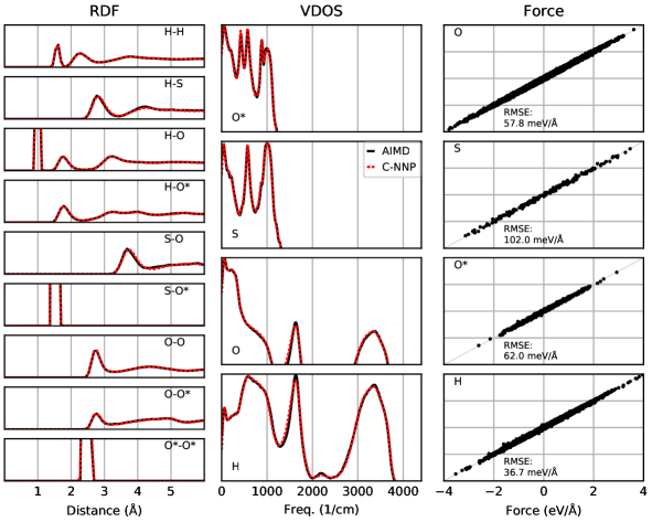
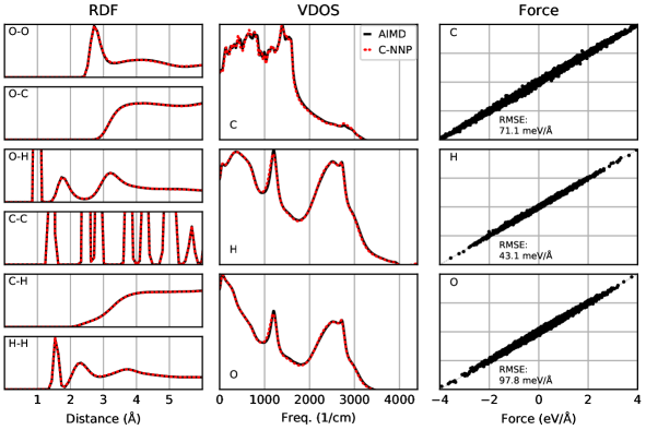
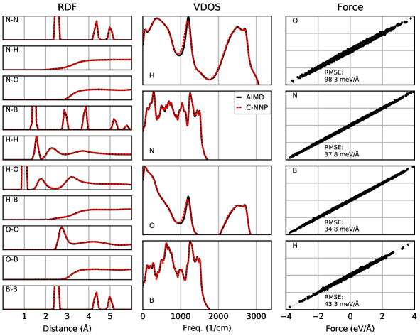
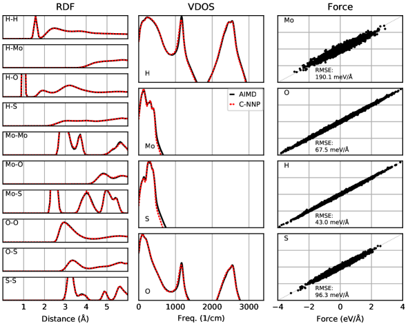
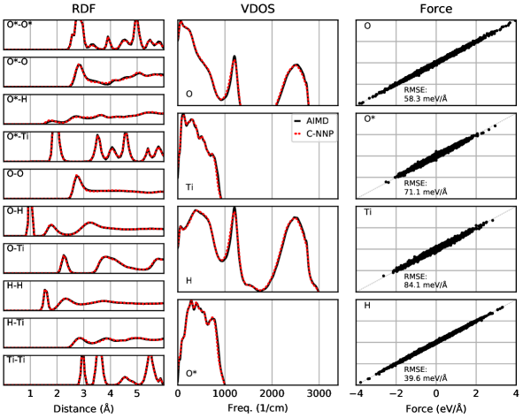
An automated training procedure calls for an efficient and robust validation protocol. Through extensive comparisons of our models to the underlying ab initio reference trajectories we have identified a general set of properties that serve to provide a stern test of our models. These can be evaluated for any system of interest and provide a broad overview of the performance of a MLP, while further tests are included in the Supporting Information. The selected properties exemplify the performance of the models for structural and dynamical properties as well as the precision of the force prediction. Specifically, the performance for structural properties is assessed by the match of the radial distribution functions (RDF) for all involved species comparing the ab initio reference to the model prediction based on molecular dynamics simulations. All RDFs of a given system provide a comprehensive summary of the structural arrangement of the system of interest and are thus ideal to evaluate the performance of the machine learning model for thermodynamic properties. Dynamical properties are validated by comparing the species-resolved vibrational density of states (VDOS) obtained with the model and the reference, which gives a comprehensive overview of inter- and intramolecular motions. Finally, the force prediction of the model is validated by the force root mean square error (RMSE) of a randomly selected subset of structures from the ab initio reference simulation. This quantity is chosen since the forces ultimately drive the molecular dynamics simulations when using the model. In order to make these properties comparable for all systems, they are reduced into a score by suitable difference measurements and subsequent averaging over the involved species as described in detail in the Supporting Information. The entire testing protocol functions in an automated manner and efficiently provides a condensed summary of the accuracy of each model.
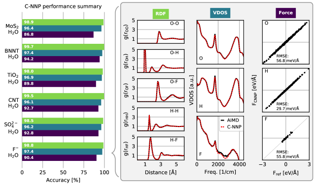
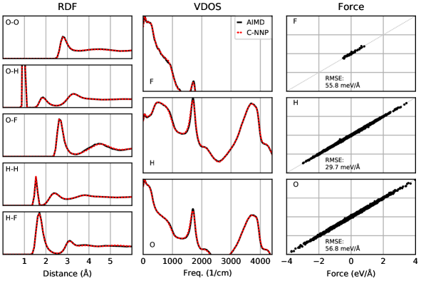
The resulting summary of the quality assessment for all six studied systems is shown in Fig. 2. From this analysis it is clear that all models reproduce the three selected properties with rather high precision, where the RDF score ranges between 100 to 98%, the VDOS score between 98 to 96%, and the force score between 95 to 86%. To illustrate the meaning of these values, we depict the individual functions (RDF and VDOS) and the force correlation for the solvated fluoride ion C-NNP model along with the total scores in Fig. 2, while all other properties for the remaining models are compiled in the Supporting Information. This comparison shows that the selected properties are reproduced with good agreement to the ab initio reference method by our six C-NNP models. In addition, all C-NNP results included in this performance summary are based on substantially extended simulation times compared to the AIMD references as described in detail in the Supporting Information. This highlights the robust nature of our models, enabling reliable predictions over long time scales. We note that statistical fluctuations due to the more converged nature of our C-NNP simulations accounts only for very minor changes of the final property scores on the order of 0.5%.
Besides the three sets of properties that we have quantitatively validated here, we have performed additional performance tests, in particular for the more complex systems of water confined in nanotubes and between \chMoS2 sheets as well as water on \chTiO2. These tests include the detailed analysis of the global structure of the solid and liquid subsystems, as encoded by the density profiles, the hydrogen bonding of water in the various systems, and the orientation of water with respect to the involved interfaces. For all these tests, which are presented in detail in the Supporting Information, we observe good agreement between our C-NNP results and the AIMD reference simulations within the statistics of those shorter AIMD runs. We are therefore confident that our performance overview, presented in Fig. 2, underlines the high quality of our C-NNP models.
The quality assessment for the six different systems included in this work clearly highlights that our simple and straightforward process to develop machine learning potentials is able to provide robust and accurate models for the selected thermodynamic condition. Compared to the typical DFT setups employed here, the evaluation of the potential energy and atomic forces is usually four to five orders of magnitude faster with the C-NNP model. As a consequence, all chosen systems could now be studied in detail using exhaustive simulations that are accessible with the developed models. Given the focus on general properties in the testing protocol, we expect that it could prove useful for the development of potentials for various other solid-liquid systems of technological and/or scientific interest.
Reaching longer length and time scales
Let us finally showcase the potential of the presented methodology to extend the length and time scales of molecular simulations and thus further the understanding of a system of interest. For that purpose we investigate structural and dynamical properties of water in contact with rutile \chTiO2(110). This system is of scientific and technological importance due to the application of \chTiO2 for example in photocatalysis or self-cleaning coatings and sensors. In addition, it is an established prototypical oxide system in surface science Pang2013/10.1021/cr300409r and a rather controversial benchmark system both for theory and experiment Diebold2017/10.1063/1.4996116. For example, the extent of the mobility of water in the contact layers, relevant e.g. for a detailed understanding of catalytic processes, has been the focus of substantial research Predota2007/10.1021/jp065165u; Liu2010/10.1103/PhysRevB.82.161415; Spencer2009/10.1021/jp8109918; English2012/10.1080/00268976.2012.683888; Agosta2017/10.1063/1.4991381.
In order to shed light on these questions, we have used the developed C-NNP model to simulate rutile \chTiO2(110) in contact with water. The model was constructed from a 30 ps AIMD simulation at 300 K with the optB88-vdW functional Klimes2010/10.1088/0953-8984/22/2/022201, involving a four O-Ti-O trilayer slab in contact with 80 water molecules, forming a 1.5 nm water film on the surface. After the development and benchmarking of the C-NNP model as shown in the previous section, we made a 22 model of the interface (resulting in a \chTiO2/H2O setup with 1728 atoms) and ran 5 ns of MD. Reaching such length and time scales with AIMD simulations would represent an enormous computational burden, while they can be routinely performed with the C-NNP models. Further details of these simulations can be found in the Materials and Methods section.
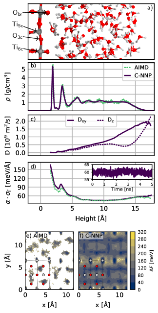
First, we analyze the water structuring by looking at the density profile of water on the \chTiO2 surface shown in panel b) of Fig. 3. The first important observation is the close match between the crude density profile obtained for our AIMD simulation and the statistically converged profile obtained with the significantly extended C-NNP simulation. Overall, we observe a highly structured arrangement of water in the first two layers, which correspond to the water adsorbed on the 5-coordinated titanium site for the first peak and the water around the 6-coordinated titanium site for the second peak, as shown in the snapshot in the top panel. This density profile is substantially more structured than for AIMD simulations of water on rutile Liu2010/10.1103/PhysRevB.82.161415 with the PBE functional, which highlights the complex dependence of interfacial properties on the chosen functional. Given the improved understanding of the dependence of the properties of water on the DFT functional, in particular regarding the inclusion of dispersion interactions Gillan2016/10.1063/1.4944633, we conclude that modern DFT approaches predict a highly structured arrangement of water on the rutile surface reaching up to about 1 nm into the liquid. This is also in good agreement with the density profiles obtained from MLP simulations of water on the anatase (101) surface Andrade2020/10.1039/c9sc05116c that used the SCAN functional as the reference method.
In a next step, we evaluate the water diffusion coefficient resolved by the distance from the \chTiO2 surface. Specifically, we make use of the mean square displacement, which we spatially decompose based on the position of each water molecule at zero delay Pluharova2019/10.1021/acs.jctc.8b00111 — an approach made feasible by the extensive statistics provided by our C-NNP model. We then obtain a local estimate of the diffusion coefficient by the well-known Einstein relation, which can be evaluated separately for the parallel (xy) and perpendicular (z) directions with respect to the interface. Panel c) in Fig. 3 depicts the resulting water diffusion constant Dxy and Dz as a function of the distance from the \chTiO2 surface. As anticipated from the very structured density profile, the mobility close to the surface is reduced substantially, where essentially no diffusion is observed in the strongly adsorbed contact layer. Beyond the first and second layer, the diffusivity in the xy-direction increases steadily up to the water-vacuum interface. At the same time, Dz features a plateau around 1 nm from the surface and a substantial increase in diffusion towards the vapor interface. Overall, this analysis highlights the strong influence of the \chTiO2 interface on the water diffusion stretching more than 1 nm into the liquid.
Next, we address the accuracy of our extended C-NNP simulations by analyzing the intrinsic error estimate of our model, given by the atomic force committee disagreement . Panel d) in Fig. 3 resolves this local error estimate of the atomic force components for all water atoms as a function of the distance from the surface. This error estimate is a product of the committee disagreement , as directly provided by our C-NNP simulations, and a scaling factor determined to match the force RMSE of a validation set as proposed in Ref. Imbalzano2021/10.1063/5.0036522. In addition, we have evaluated this error estimate with our C-NNP model for all configurations of the original AIMD simulation to assess if the increased system size or C-NNP generated structures lead to higher errors. Overall, we observe error estimates between 40 to 80 meV/Å over the entire water region with only slightly higher values close to the \chTiO2 surface, indicating the increased complexity of the involved interactions in this inhomogeneous region. Furthermore, the error (averaged over all water atoms) does not deteriorate over the course of the 5 ns long trajectory, fluctuating around an average of 60 meV/Å, as shown in the inset of panel d). Such atomic force errors are similar or even smaller than those reported for other developed MLPs e.g. for pure water Morawietz2016/10.1073/pnas.1602375113; Cheng2019/10.1073/pnas.1815117116; Gartner2020/10.1073/pnas.2015440117; Schran2020/10.1063/5.0016004. At the same time, the error estimate obtained for the AIMD configurations features essentially the same distance resolved profile, which reveals that our C-NNP simulations are able to conserve their predictive power, while substantially extending both time and length scales of the simulations.
Finally, we analyze the free energy profile of water adsorbed in the first two contact layers on the \chTiO2 surface, as depicted in panels e) and f) in Fig. 3 for the AIMD and C-NNP simulation, respectively. From the direct comparison between the AIMD and C-NNP results it is clear that the limited statistics of the shorter AIMD simulation is insufficient to provide reliable insight into this property. Only with the extensive sampling enabled by the C-NNP model, the free energy profile can be fully converged. The C-NNP free energy profile clearly underlines the strong preference for water adsorption above the fivefold coordinated titanium sites in the first contact layer and the slightly weaker adsorption of water around the sixfold coordinated titanium and threefold coordinated oxygen sites in the second contact layer. In between these adsorption sites, substantial free energy barriers are observed, highlighting the immobile nature of the two contact layers as also revealed by the analysis of the water diffusion.
In summary, the extensive simulations with our C-NNP model, obtained in a straightforward and efficient workflow, provide detailed insight into the properties of water on the rutile surface. We observe a pronounced water layering effect with strong density fluctuations and clear evidence of a highly structured arrangement of water in the first adsorption layers. In addition, our analysis of the water dynamics reveals almost no water diffusion close to the interface and a strong influence on the diffusion stretching more than 1 nm into the liquid. The treatment of a complex interfacial system such as this one requires an accurate description of the binding at the various adsorption sites as well as long-time sampling of the dynamics. The C-NNP model developed here delivers on both fronts, which highlights the potential of our approach to deepen understanding of technologically relevant solid-liquid systems.
Conclusion
In this work, we have presented a machine learning framework that makes the generation of MLPs simple. We have also showcased its versatility for the description of a range of complex aqueous systems. Making use of committee neural network potentials, we have shown how MLPs can be obtained in a straightforward and robust process from a single reference simulation. By essentially removing the need to adjust any hyperparameters, a new system of interest can be tackled in a direct, data-driven way. We have demonstrated the potential of this approach employing it for six complex liquid and solid-liquid systems and have evaluated the quality of the resulting models in detail for various properties underlining the high accuracy of our models. This important final step is realized with an automated validation protocol that is fully integrated into our framework. These developments are directly accessible to the community as they build exclusively on open-source solutions and we make our underlying software package and all templates available.
In its spirit similar to on-the-fly learning techniques, we depart from the goal of a high degree of transferability or generality to concentrate exclusively on the thermodynamic condition relevant for the chosen scientific question. Under these constraints, we have shown how a robust and accurate machine learning potential can be obtained with limited user input in an uncomplicated process. We note that we have also explored the application of our models for elevated and lowered temperatures, which was possible without problems in a 30 K regime. During such simulations, the intrinsic error estimate of our approach is a very useful tool to gauge the validity of the results. Due to these promising signs, we plan to systematically validate the robustness of our models to venture beyond the chosen thermodynamic state point, for example to describe variations in pressure.
We note that we built our development on established components, such as an efficient ML structure-energy representation and active learning concepts. At the same time, we expect that the concepts laid out in this work are transferable to other MLPs and active learning approaches, making it possible to achieve similar results. The novelty of our work lies in a change in perspective, where relatively little effort is put into creating an intermolecular potential which, in spite of concentrating on a sub-section of phase space, is still robust and accurate enough to be used to describe the non-trivial behavior of complex molecular systems. The importance clearly is not in the individual pieces but rather in the end-to-end framework and the broad range of applications made possible. This work therefore enables simulations that were not possible a short time ago, pushing forward the straightforward and reliable application of MLPs.
Looking to the future, we have limited ourselves to aqueous systems with four species in this work. However, we are confident that systems with more element types can also be tackled with our approach. In addition, we have not explored reactive processes in this study. Since MLPs are able to describe bond breaking and bond making events by design, we again anticipate the straightforward application of our methodology to such situations. This will be especially important to investigate interesting surface reaction phenomena, such as water dissociation on reactive surfaces or the recently reported reversible hydrolysis of zeolites in contact with water Heard2019/10.1038/s41467-019-12752-y. Key to a successful application in such situations will be the sampling of the relevant reactive process by the initial AIMD simulation used as input to our active learning protocol. Finally, we are currently exploring a training protocol in which structures are generated by classical molecular dynamics as input for our active learning protocol to minimize the need for expensive ab initio calculations. In this approach the expensive quantum computing engine is only used to obtain the ab initio potential energies and atomic forces for those configurations identified to be most important for the generation of the model. Such an approach has potential for additional cost savings over the one presented here and does not require expertise in AIMD simulations, thus more readily opening up the approach to researchers from the classical force field community.
In our six showcase applications of complex aqueous systems we have developed models with different DFT functionals, all of which represent reasonable choices for the aqueous systems studied. However, this illustrates a broader issue which is that there is currently no ‘perfect’ DFT functional for water and complex aqueous interfaces. We believe that the approach developed here could become a valuable tool in this long-standing quest to find suitable DFT functionals. Since our procedures provide the ability to reveal the true converged thermal performance of any given functional for a realistic system, at a modest cost, the systematic exploration of the performance of DFT methods for complex disordered systems becomes feasible. This makes it possible to go beyond the usual energetic benchmarks of relatively small systems in the absence of temperature and thus facilitates direct comparison with experiment. Due to the moderate size of our training sets, our framework is also expected to be easily extendable to more expensive ab initio methods, e.g. at the hybrid DFT level or considering explicit electron correlation, thus making these methods available for the realistic simulation of complex interfacial systems.
Overall, the developments reported herein will enable the investigation of complex aqueous processes such as water structuring in contact with interfaces and wetting or ice formation on surfaces in a straightforward manner. Although here we applied it to aqueous systems, we believe that the methodology will also prove useful for other materials and liquids in contact with solids, as well as general solvation phenomena, enabling the fast screening of different materials at ab initio accuracy. It will also be particularly useful for situations where long sampling is required as for the exploration of free energy surfaces, or calculations of dynamical properties, such as the friction or viscosity of liquids in contact with interfaces. In summary, this work outlines a straightforward strategy for the uncomplicated yet accurate investigation of many technologically and scientifically relevant systems by molecular simulations.
Materials and Methods
The introduced machine learning framework has been implemented in the AML Python package, which interleaves the required simulation packages and data manipulation steps in a user friendly environment. The AML package is available free of charge at https://github.com/MarsalekGroup/aml and enables the straightforward generation of a C-NNP model given a reference trajectory as input. With this code all six C-NNP models were developed for the various aqueous phase systems studied here.
NNP optimizations were performed with the open-source n2p2 code Singraber2019/10.1021/acs.jctc.8b01092 using the optimization parameters and symmetry functions as provided in the template file in the associated data repository for this paper. All additional information on the C-NNP fitting procedure can be found in the SI, while all training input files, training sets and parameters of the final models are publicly available at https://github.com/water-ice-group/simple-MLP.
The reference AIMD simulations used as the starting point for our C-NNP models employed quite different DFT settings, while all having been performed with the CP2K simulation package Kuhne2020/10.1063/5.0007045. We provide full detail about these reference simulations in the SI, but the typical simulation setups consist of 64 to 110 water molecules reaching simulation times between 30 to 130 ps.
MD simulations using the C-NNP models were also performed with CP2K, which features an open-source implementation of the C-NNP methodology since release 8.1. All C-NNP simulations for our validation protocol were propagated for at least 0.5 ns to allow for the converged computation of the RDF and VDOS. Further details of the validation protocol and the associated simulations can be found in the SI, while the validation can be performed with the AML Python package. The C-NNP simulations of the \chTiO2 water system were propagated for 5 ns for a 221 supercell of the original AIMD setup, resulting in total in 1728 atoms making up 320 water molecules on four O-Ti-O trilayers in a 23.672, 25.988, 42.0 Å periodic box. This simulation employed a molecular dynamics time step of 1 fs, while using deuterium masses for the hydrogen atoms. The temperature of 300 K was maintained with a canonical sampling through velocity rescaling thermostat Bussi2007/10.1063/1.2408420.
Acknowledgements.
We would like to thank Christopher Penschke for providing the water \chTiO2 AIMD trajectory. C.S. acknowledges partial financial support from the Alexander von Humboldt-Stiftung. This work was partially supported by the OP RDE project (No. CZ.02.2.69/0.0/0.0/18_070/0010462), International mobility of researchers at Charles University (MSCA- IF II). We are grateful to the UK Materials and Molecular Modelling Hub for computational resources, which is partially funded by EPSRC (EP/P020194/1 and EP/T022213/1). We are also grateful for computational support from the UK national high performance computing service, ARCHER, for which access was obtained via the UKCP consortium, funded by EPSRC grant ref EP/P022561/1.References
- Zaera (2012) F. Zaera, Chem. Rev. 112, 2920 (2012).
- Björneholm et al. (2016) O. Björneholm, M. H. Hansen, A. Hodgson, L. M. Liu, D. T. Limmer, A. Michaelides, P. Pedevilla, J. Rossmeisl, H. Shen, G. Tocci, E. Tyrode, M. M. Walz, J. Werner, and H. Bluhm, Chem. Rev. 116, 7698 (2016).
- Behler (2016) J. Behler, J. Chem. Phys. 145, 170901 (2016).
- Butler et al. (2018) K. T. Butler, D. W. Davies, H. Cartwright, O. Isayev, and A. Walsh, Nature 559, 547 (2018).
- Deringer, Caro, and Csányi (2019) V. L. Deringer, M. A. Caro, and G. Csányi, Adv. Mater. 31, 1902765 (2019).
- Kang, Shang, and Liu (2020) P. L. Kang, C. Shang, and Z. P. Liu, Acc. Chem. Res. 53, 2119 (2020).
- Behler (2021) J. Behler, Chem. Rev. (2021), 10.1021/acs.chemrev.0c00868.
- Morawietz et al. (2016) T. Morawietz, A. Singraber, C. Dellago, and J. Behler, Proc. Natl. Acad. Sci. 113, 8368 (2016).
- Cheng et al. (2019) B. Cheng, E. A. Engel, J. Behler, C. Dellago, and M. Ceriotti, Proc. Natl. Acad. Sci. 116, 1110 (2019), arXiv:1811.08630 .
- Gartner et al. (2020) T. E. Gartner, L. Zhang, P. M. Piaggi, R. Car, A. Z. Panagiotopoulo, and P. G. Debenedet, Proc. Natl. Acad. Sci. 117, 26040 (2020).
- Deringer et al. (2021) V. L. Deringer, N. Bernstein, G. Csányi, C. Ben Mahmoud, M. Ceriotti, M. Wilson, D. A. Drabold, and S. R. Elliott, Nature 589, 59 (2021).
- Jinnouchi et al. (2019) R. Jinnouchi, J. Lahnsteiner, F. Karsai, G. Kresse, and M. Bokdam, Phys. Rev. Lett. 122, 225701 (2019), arXiv:1903.09613 .
- Behler and Parrinello (2007) J. Behler and M. Parrinello, Phys. Rev. Lett. 98, 146401 (2007).
- Ghasemi et al. (2015) S. A. Ghasemi, A. Hofstetter, S. Saha, and S. Goedecker, Phys. Rev. B 92, 045131 (2015), arXiv:1501.07344 .
- Schütt et al. (2017) K. T. Schütt, F. Arbabzadah, S. Chmiela, K. R. Müller, and A. Tkatchenko, Nat. Commun. 8, 13890 (2017), arXiv:1609.08259 .
- Zhang et al. (2018) L. Zhang, J. Han, H. Wang, R. Car, and E. Weinan, Phys. Rev. Lett. 120, 143001 (2018), arXiv:1707.09571 .
- Unke and Meuwly (2019) O. T. Unke and M. Meuwly, J. Chem. Theory Comput. 15, 3678 (2019), arXiv:1902.08408 .
- Bartók et al. (2010) A. P. Bartók, M. C. Payne, R. Kondor, and G. Csányi, Phys. Rev. Lett. 104, 136403 (2010).
- Rupp et al. (2012) M. Rupp, A. Tkatchenko, K. R. Müller, and O. A. Von Lilienfeld, Phys. Rev. Lett. 108, 058301 (2012).
- Thompson et al. (2015) A. Thompson, L. Swiler, C. Trott, S. Foiles, and G. Tucker, J. Comput. Phys. 285, 316 (2015).
- Shapeev (2015) A. V. Shapeev, Multiscale Model. Simul. 14, 1153 (2015).
- Li, Kermode, and De Vita (2015) Z. Li, J. R. Kermode, and A. De Vita, Phys. Rev. Lett. 114, 096405 (2015).
- Chmiela et al. (2017) S. Chmiela, A. Tkatchenko, H. E. Sauceda, I. Poltavsky, K. T. Schütt, and K. R. Müller, Sci. Adv. 3, e1603015 (2017), arXiv:1611.04678 .
- Gastegger, Behler, and Marquetand (2017) M. Gastegger, J. Behler, and P. Marquetand, Chem. Sci. 8, 6924 (2017).
- Podryabinkin and Shapeev (2017) E. V. Podryabinkin and A. V. Shapeev, Comput. Mater. Sci. 140, 171 (2017).
- Zhang et al. (2019) L. Zhang, D.-Y. Lin, H. Wang, R. Car, and W. E, Phys. Rev. Mater. 3, 023804 (2019), arXiv:1810.11890 .
- Smith et al. (2018) J. S. Smith, B. Nebgen, N. Lubbers, O. Isayev, and A. E. Roitberg, J. Chem. Phys. 148, 241733 (2018), arXiv:1801.09319 .
- Deringer, Pickard, and Csányi (2018) V. L. Deringer, C. J. Pickard, and G. Csányi, Phys. Rev. Lett. 120, 156001 (2018), arXiv:1710.10475 .
- Schütt et al. (2018) K. T. Schütt, H. E. Sauceda, P. J. Kindermans, A. Tkatchenko, and K. R. Müller, J. Chem. Phys. 148, 241722 (2018), arXiv:1712.06113 .
- Musil et al. (2018) F. Musil, S. De, J. Yang, J. E. Campbell, G. M. Day, and M. Ceriotti, Chem. Sci. 9, 1289 (2018).
- Schran, Behler, and Marx (2020) C. Schran, J. Behler, and D. Marx, J. Chem. Theory Comput. 16, 88 (2020), arXiv:1908.08734 .
- Bartók et al. (2018) A. P. Bartók, J. Kermode, N. Bernstein, and G. Csányi, Phys. Rev. X 8, 041048 (2018), arXiv:1805.01568 .
- Rowe et al. (2020) P. Rowe, V. L. Deringer, P. Gasparotto, G. Csányi, and A. Michaelides, J. Chem. Phys. 153, 034702 (2020), arXiv:2006.13655 .
- Deringer, Caro, and Csányi (2020) V. L. Deringer, M. A. Caro, and G. Csányi, Nat. Commun. 11, 1 (2020).
- Natarajan and Behler (2016) S. K. Natarajan and J. Behler, Phys. Chem. Chem. Phys. 18, 28704 (2016).
- Hellström, Quaranta, and Behler (2019) M. Hellström, V. Quaranta, and J. Behler, Chem. Sci. 10, 1232 (2019).
- Andrade et al. (2020) M. F. Andrade, H. Y. Ko, L. Zhang, R. Car, and A. Selloni, Chem. Sci. 11, 2335 (2020).
- Ghorbanfekr, Behler, and Peeters (2020) H. Ghorbanfekr, J. Behler, and F. M. Peeters, J. Phys. Chem. Lett. 11, 7363 (2020).
- Artrith (2019) N. Artrith, “Machine learning for the modeling of interfaces in energy storage and conversion materials,” (2019).
- Jinnouchi et al. (2020) R. Jinnouchi, K. Miwa, F. Karsai, G. Kresse, and R. Asahi, J. Phys. Chem. Lett. 11, 6946 (2020).
- Vandermause et al. (2020) J. Vandermause, S. B. Torrisi, S. Batzner, Y. Xie, L. Sun, A. M. Kolpak, and B. Kozinsky, npj Comput. Mater. 6, 1 (2020).
- Bisbo and Hammer (2020) M. K. Bisbo and B. Hammer, Phys. Rev. Lett. 124, 086102 (2020), arXiv:1907.05741 .
- Schran, Brezina, and Marsalek (2020) C. Schran, K. Brezina, and O. Marsalek, J. Chem. Phys. 153, 104105 (2020), arXiv:2006.01541 .
- Behler (2017) J. Behler, Angew. Chemie - Int. Ed. 56, 12828 (2017).
- Artrith, Morawietz, and Behler (2011) N. Artrith, T. Morawietz, and J. Behler, Phys. Rev. B 83, 153101 (2011).
- Grisafi and Ceriotti (2019) A. Grisafi and M. Ceriotti, J. Chem. Phys. 151, 204105 (2019), arXiv:1909.04512 .
- Ko et al. (2021) T. W. Ko, J. A. Finkler, S. Goedecker, and J. Behler, Nat. Commun. 12, 1 (2021), arXiv:2009.06484 .
- Yue et al. (2021) S. Yue, M. C. Muniz, M. F. Andrade, L. Zhang, R. Car, and A. Z. Panagiotopoulos, J. Chem. Phys. 154, 034111 (2021).
- Imbalzano et al. (2021) G. Imbalzano, Y. Zhuang, V. Kapil, K. Rossi, E. A. Engel, F. Grasselli, and M. Ceriotti, J. Chem. Phys. 154, 074102 (2021), arXiv:2011.08828 .
- Behler (2011) J. Behler, J. Chem. Phys. 134, 074106 (2011).
- Grossman et al. (2004) J. C. Grossman, E. Schwegler, E. W. Draeger, F. Gygi, and G. Galli, J. Chem. Phys. 120, 300 (2004).
- Distasio et al. (2014) R. A. Distasio, B. Santra, Z. Li, X. Wu, and R. Car, J. Chem. Phys. 141, 084502 (2014), arXiv:1405.5265 .
- Forster-Tonigold and Groß (2014) K. Forster-Tonigold and A. Groß, J. Chem. Phys. 141, 064501 (2014).
- Gillan, Alfè, and Michaelides (2016) M. J. Gillan, D. Alfè, and A. Michaelides, J. Chem. Phys. 144, 130901 (2016), arXiv:1603.01990 .
- Chen et al. (2017) M. Chen, H. Y. Ko, R. C. Remsing, M. F. Calegari Andrade, B. Santra, Z. Sun, A. Selloni, R. Car, M. L. Klein, J. P. Perdew, and X. Wu, Proc. Natl. Acad. Sci. 114, 10846 (2017), arXiv:1709.10493 .
- Marsalek and Markland (2017) O. Marsalek and T. E. Markland, J. Phys. Chem. Lett. 8, 1545 (2017), arXiv:1702.07797 .
- Brandenburg et al. (2019) J. G. Brandenburg, A. Zen, D. Alfè, and A. Michaelides, J. Chem. Phys. 151 (2019), 10.1063/1.5121370, arXiv:1907.09525 .
- Schienbein and Marx (2020) P. Schienbein and D. Marx, Angew. Chemie - Int. Ed. 59, 18578 (2020).
- Sharkas et al. (2020) K. Sharkas, K. Wagle, B. Santra, S. Akter, R. R. Zope, T. Baruah, K. A. Jackson, J. P. Perdew, and J. E. Peralta, Proc. Natl. Acad. Sci. 117, 11283 (2020).
- Wagle et al. (2021) K. Wagle, B. Santra, P. Bhattarai, C. Shahi, M. R. Pederson, K. A. Jackson, and J. P. Perdew, J. Chem. Phys. 154, 094302 (2021), arXiv:2012.13469 .
- Duignan et al. (2021) T. T. Duignan, S. M. Kathmann, G. K. Schenter, and C. J. Mundy, Acc. Chem. Res. 147, 47 (2021).
- Pang, Lindsay, and Thornton (2013) C. L. Pang, R. Lindsay, and G. Thornton, Chem. Rev. 113, 3887 (2013).
- Diebold (2017) U. Diebold, J. Chem. Phys. 147, 040901 (2017).
- Předota, Cummings, and Wesolowski (2007) M. Předota, P. T. Cummings, and D. J. Wesolowski, J. Phys. Chem. C 111, 3071 (2007).
- Liu et al. (2010) L. M. Liu, C. Zhang, G. Thornton, and A. Michaelides, Phys. Rev. B 82, 161415 (2010).
- Spencer et al. (2009) E. C. Spencer, A. A. Levchenko, N. L. Ross, A. I. Kolesnikov, J. Boerio-Goates, B. F. Woodfield, A. Navrotsky, and G. Li, J. Phys. Chem. A 113, 2796 (2009).
- English, Kavathekar, and MacElroy (2012) N. J. English, R. S. Kavathekar, and J. M. MacElroy, Mol. Phys. 110, 2919 (2012).
- Agosta, Brandt, and Lyubartsev (2017) L. Agosta, E. G. Brandt, and A. P. Lyubartsev, J. Chem. Phys. 147 (2017), 10.1063/1.4991381.
- Klimeš, Bowler, and Michaelides (2010) J. Klimeš, D. R. Bowler, and A. Michaelides, J. Phys. Condens. Matter 22, 022201 (2010), arXiv:0910.0438 .
- Pluhařová et al. (2019) E. Pluhařová, P. Jungwirth, N. Matubayasi, and O. Marsalek, J. Chem. Theory Comput. 15, 803-812 (2019).
- Heard et al. (2019) C. J. Heard, L. Grajciar, C. M. Rice, S. M. Pugh, P. Nachtigall, S. E. Ashbrook, and R. E. Morris, Nat. Commun. 10, 1 (2019).
- Singraber et al. (2019) A. Singraber, T. Morawietz, J. Behler, and C. Dellago, J. Chem. Theory Comput. 15, 3075 (2019).
- Kühne et al. (2020) T. D. Kühne, M. Iannuzzi, M. Del Ben, V. V. Rybkin, P. Seewald, F. Stein, T. Laino, R. Z. Khaliullin, O. Schütt, F. Schiffmann, D. Golze, J. Wilhelm, S. Chulkov, M. H. Bani-Hashemian, V. Weber, U. Borštnik, M. Taillefumier, A. S. Jakobovits, A. Lazzaro, H. Pabst, T. Müller, R. Schade, M. Guidon, S. Andermatt, N. Holmberg, G. K. Schenter, A. Hehn, A. Bussy, F. Belleflamme, G. Tabacchi, A. Glöß, M. Lass, I. Bethune, C. J. Mundy, C. Plessl, M. Watkins, J. VandeVondele, M. Krack, and J. Hutter, J. Chem. Phys. 152, 194103 (2020), arXiv:2003.03868 .
- Bussi, Donadio, and Parrinello (2007) G. Bussi, D. Donadio, and M. Parrinello, J. Chem. Phys. 126, 014101 (2007), arXiv:0803.4060 .
Supporting information for: Machine learning potentials for complex aqueous systems made simple
Quality assessment
In order to validate the six models developed by our rapid machine learning framework, we have established a validation protocol that makes it possible to compare the performance of the various models for different systems in a direct and condensed manner. For that purpose we have selected three main categories for structural and dynamical properties as well as the precision of the force prediction. The main idea behind this validation protocol is that it probes the performance of a given model for the thermodynamic condition it is developed for. Thus, all three categories are compared directly against the AIMD simulation that was used as the starting point of the development of the models. This enables the straight-forward evaluation of the models without the need for additional benchmark simulations with the expensive reference method.
Structural properties for complex liquid-solid systems are directly probed by the radial distribution functions (RDFs) of the various species, which provide detailed insight into the two-component structural arrangement. For the scoring of the models, we compute all RDFs for a given system, both for the AIMD reference simulation and for independent C-NNP simulations using the developed model. For an component system this results in RDFs which can be directly compared between the AIMD and C-NNP results by using a suitable norm
| (S1) |
which provides a measure of the similarity of two RDFs ranging from 0 (for most different) to 1 (for identical). Averaging over all norms finally yields a single number that can be converted into percent to provide a condensed score for the performance of the C-NNP model for structural properties.
Dynamical properties are directly encoded by the vibrational density of states (VDOS), which is obtained by Fourier transform of the velocity autocorrelation function. The VDOS can be computed separately for all components in a system of interest and thus provides detailed insight into the dynamical properties of the system, probing vastly different processes over a broad frequency range. For an component system species-resolved VDOS are computed, both for the AIMD and C-NNP simulations. Using a similar norm as for the RDFs
| (S2) |
the AIMD and C-NNP results can be condensed into a measure of the similarity between the different functions, which after averaging over the different species and conversion into percent provides the score of a C-NNP model for dynamical properties.
Finally, the precision of the C-NNP model for the prediction of the forces is evaluated to provide another property score. The forces are what drives the dynamics of the system of interest and are thus of fundamental importance for an accurate description. We generated a test set for the evaluation of the force performance, by selecting a large subset of 1000 structures and associated forces from the original AIMD simulation. The root mean square error (RMSE), calculated separately for the species in each system
| (S3) |
is used as a suitable measure for the force prediction. Since the magnitude of the forces can fluctuate strongly for different systems, but also within a given system (solid compared to liquid atoms), the RMSE is put into relation of the average force fluctuation of a given species
| (S4) |
The resulting scaled force errors are averaged and converted into percent to provide the force score of the C-NNP model.
Properties evaluated for Quality Assessment
All individual properties evaluated for the validation protocol comprising the final RDF, VDOS, and force score, as presented in the main text, are shown in full detail for all six C-NNP models in Fig. S1 to Fig. S6. Overall, essentially perfect agreement between the AIMD and C-NNP properties is observed for all six systems.
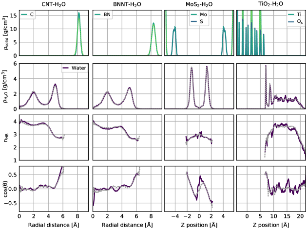
In addition, we have evaluated other properties for the systems of water under confinement or at interfaces in order to validate our C-NNP models in more detail. These properties are the density profiles, number of hydrogen bonds, and water orientation with respect to the interfaces for the \chCNT-H2O, \chBNNT-H2O, \chMoS-H2O, and \chTiO2-H2O systems. They are all depict in Fig. S7 where overall substantial agreement between the C-NNP prediction and the much shorter AIMD reference simulations is observed. In particular, the density profile of the liquid and solid subsystems as shown in the upper two columns highlight the different nature of confinement with distinct density modulations that are all well reproduced by our C-NNP models. In addition, the number of hydrogen bonds along the water density profile is in substantial agreement between AIMD reference and C-NNP prediction for all four systems. Finally, the orientation of water with respect to the involved interfaces, as encoded by the cosine of the angle between the water dipole vector and the normal of the interface, is also well reproduced by our C-NNP models.
Computational Details
C-NNP models
All C-NNP models for the six selected systems were trained with the active learning workflow implemented in the AML Python package, available at https://github.com/MarsalekGroup/aml.
Using an ab initio trajectory as input, we construct a C-NNP model and its associated training set in an active learning protocol. 20 randomly selected structures from the trajectory are used to generate an initial C-NNP model. Next, the model is improved by iteratively adding structures with largest mean force committee disagreement to the training set, which is continued until convergence of the committee disagreement is observed. We performed 15 such active learning steps for all systems studied here, identifying 20 new structures for the training set in every step, but keeping out previously selected structures, which results in a total training set size of about 300 structures. Within every active learning step, the committee disagreement of 2000 randomly selected structures from the AIMD reference trajectory is evaluated and the 20 structures with largest mean force disagreement are added to the training set. The final C-NNP models are then obtained after stringent training of the NNP members with tight convergence criteria, as mentioned below in detail.
The chemical environment around each atom is described by a set of atom–centered symmetry functions Behler2011/10.1063/1.3553717, which transform the structure into suitable input for the atomic NNs. We applied a general set of symmetry functions to all systems studied here that can be automatically generated for a new system of interest within the AML package. The structural information for angular and radial symmetry functions is restricted to a radial cutoff of 12 bohr by a cosine cutoff function. For every pair of elements we employ ten radial symmetry functions, with fixed Gaussian width of 0.308 bohr, which are equally distributed within the 12 bohr cutoff. For every triple of elements we use four angular symmetry functions with a fixed Gaussian width of 0.012 bohr, and of 1 and 4, respectively. All symmetry function values are scaled and centered based on the average and range of the individual symmetry functions encountered in the training set according to
| (S5) |
All NNs consist of two hidden layers with 20 neurons, while the hyperbolic tangent was used as activation function for all layers, except the output neuron, which features a linear activation function. NNP optimizations are performed with the open-source n2p2 code Singraber2019/10.1021/acs.jctc.8b01092 and the optimization parameters have been chosen according to the detailed benchmarking of this code for water Singraber2019/10.1021/acs.jctc.8b01092.
Each C-NNP model is made up of 8 NNP members, which are constructed by random subsampling of the full reference data, where 10% of the points are left out in each case to impose the required diversity between C-NNP members. After different random initialization for each committee member, the weights and biases of the NNs were optimized using the parallel multistream version Singraber2019/10.1021/acs.jctc.8b01092 of the adaptive global extended Kalman filter as implemented in n2p2. C-NNPs used for QbC were optimized for 15 epochs with 6 streams, while the final C-NNPs, to be used for simulations, were optimized for 50 epochs with 24 streams. All training input files, training sets and parameters of the final models are publicly available at https://github.com/water-ice-group/simple-MLP.
AIMD simulations
All ab initio molecular dynamics simulations used as input for our machine learning framework haven been performed with the CP2K software package Kuhne2020/10.1063/5.0007045.
The fluoride ion in water was described at the hybrid DFT level with the revPBE0 functional and D3 dispersion correction. The wavefunction was represented up to a plane wave cutoff of 400 Ry in conjunction with the TZV2P basis set and GTH pseudopotentials. The Hartree-Fock exchange calculation is speed up using the auxiliary density matrix methods as implemented in C2PK. A single fluoride ion was described in a periodic box of 64 water molecules with a cell size of 12.445 Å. The system was propagated in the NVT ensemble at 300 K with a molecular dynamics timestep of 0.5 fs. Equilbiration with a CSVR thermostat and 30 fs coupling constant was performed for 3 ps, while the temperature for the 50 ps production run was maintained with a CSVR thermostat and 1 ps coupling constant.
The sulfate ion in water was described with the BLYP functional in combination with the D3 dispersion correction. A plane wave cutoff of 280 Ry was used, while the molecularly optimized TZV2P atomic basis set was employed for all elements in combination with GTH pseudopotentials. The system contains a single sulfate ion and 64 water molecules in a 12.41 Å periodic box. This setup was simulated in the NVT ensemble with a time step of 0.5 fs, while the temperature was maintained with a CSVR thermostat with a 50 fs coupling constant. Equilibration was performed for 5 ps followed by a 30 ps production run. This simulation has been used in a previous study on the effects of polarization for the properties of the sulfate ion Pegado2012/10.1039/c2cp40711f.
Simulations of water confined in carbon and hexagonal boron nitride nanotubes were performed for (12,12) armchair nanotubes with a length of 3 unit cells at a water density of 1.0 . This results in 288 wall atoms and 65 water molecules for the carbon nanotube and 68 water molecules for the hexagonal boron nitride nanotube. The PBE functional with D3 dispersion correction was used, in combination with GTH pseudopotentials, a 460 Ry plane wave cutoff and the DZVP molecularly optimised basis set. Deuterium masses were used for the hydrogen atoms and the molecular dynamics time step was set to 1.0 fs. Systems were pre-equilibrated for 5 ps at a temperature of 500 K using velocity rescaling, while keeping the positions of the atoms in the confining nanotubes fixed. Production runs in the NVT ensemble were then performed using Langevin dynamics, at a temperature of 330 K. Statistics were collected for approximately 130 ps for each system.
For water confined within molybdenum disulphide, the ab initio reference simulation consists of 109 water molecules confined by single layer \chMoS2 sheets of 168 atoms in a 22.545, 22.314, 11.500 Å periodic box. The optB88-vdW functional was used, with GTH pseudopotentials, a 550 Ry plane wave cutoff, a relative cutoff of 60 Ry and the DZVP molecularly optimised basis set for all elements. Equilibration was performed in the NVT ensemble, with a Nosé-Hoover chain thermostats of length 5 to maintain a temperature of 500 K for 5 ps. This was followed by a second equilibration stage at 400 K for a further 5 ps. Final data collection was performed at 400 K over a 30 ps period.
Water on the rutile titanium dioxide (110) surface was described by a system consisting of 80 water molecules on four O-Ti-O trilayers in a periodic box of dimension 11.836, 12.9938, 42.00 Å. This results in a 1.5 nm thick water film on the four trilayers with additional 15 Å vacuum to separate the periodic images in z-direction. The optB88-vdW functional was used in combination with GTH pseudopotential, a 400 Ry plane wave cutoff and the DZVP molecularly optimised basis set for all elements. After equilibration, the system was propagated for 30 ps in the NVT ensemble at 300 K maintained by a Nosé-Hoover chain thermostat of length 4 with a coupling constant of 40 fs. A 1.0 fs timestep in combination with deuterium masses for hydrogen atoms was used and the atoms of the lowest O-Ti-O trilayer — not in contact with water — were kept fixed.
References
References
- Behler (2011) J. Behler, J. Chem. Phys. 134, 074106 (2011).
- Singraber et al. (2019) A. Singraber, T. Morawietz, J. Behler, and C. Dellago, J. Chem. Theory Comput. 15, 3075 (2019).
- Kühne et al. (2020) T. D. Kühne, M. Iannuzzi, M. Del Ben, V. V. Rybkin, P. Seewald, F. Stein, T. Laino, R. Z. Khaliullin, O. Schütt, F. Schiffmann, D. Golze, J. Wilhelm, S. Chulkov, M. H. Bani-Hashemian, V. Weber, U. Borštnik, M. Taillefumier, A. S. Jakobovits, A. Lazzaro, H. Pabst, T. Müller, R. Schade, M. Guidon, S. Andermatt, N. Holmberg, G. K. Schenter, A. Hehn, A. Bussy, F. Belleflamme, G. Tabacchi, A. Glöß, M. Lass, I. Bethune, C. J. Mundy, C. Plessl, M. Watkins, J. VandeVondele, M. Krack, and J. Hutter, J. Chem. Phys. 152, 194103 (2020), arXiv:2003.03868 .
- Pegado et al. (2012) L. Pegado, O. Marsalek, P. Jungwirth, and E. Wernersson, Phys. Chem. Chem. Phys. 14, 10248 (2012).