MAESTRO: An Adaptive Low Mach Number Hydrodynamics Algorithm for Stellar Flows
Abstract
Many astrophysical phenomena are highly subsonic, requiring specialized numerical methods suitable for long-time integration. In a series of earlier papers we described the development of MAESTRO, a low Mach number stellar hydrodynamics code that can be used to simulate long-time, low-speed flows that would be prohibitively expensive to model using traditional compressible codes. MAESTRO is based on an equation set derived using low Mach number asymptotics; this equation set does not explicitly track acoustic waves and thus allows a significant increase in the time step. MAESTRO is suitable for two- and three-dimensional local atmospheric flows as well as three-dimensional full-star flows. Here, we continue the development of MAESTRO by incorporating adaptive mesh refinement (AMR). The primary difference between MAESTRO and other structured grid AMR approaches for incompressible and low Mach number flows is the presence of the time-dependent base state, whose evolution is coupled to the evolution of the full solution. We also describe how to incorporate the expansion of the base state for full-star flows, which involves a novel mapping technique between the one-dimensional base state and the Cartesian grid, as well as a number of overall improvements to the algorithm. We examine the efficiency and accuracy of our adaptive code, and demonstrate that it is suitable for further study of our initial scientific application, the convective phase of Type Ia supernovae.
1 Introduction
Many astrophysical phenomena of interest occur in the low Mach number regime, where the characteristic fluid velocity is small compared to the speed of sound. Some well-known examples are the convective phase of Type Ia supernovae (SN Ia) (Höflich & Stein, 2002; Kuhlen et al., 2006; Zingale et al., 2009), classical novae (Glasner et al., 2007), convection in stars (Meakin & Arnett, 2007), and Type I X-ray bursts (Lin et al., 2006). Such problems require a numerical approach capable of resolving phenomena over time scales much longer than the characteristic time required for an acoustic wave to propagate across the computational domain. In a series of papers (see Almgren et al. (2006a)—henceforth Paper I, Almgren et al. (2006b)—henceforth Paper II, Almgren et al. (2008)—henceforth Paper III, and Zingale et al. (2009)—henceforth Paper IV), we have described the initial development of MAESTRO, a low Mach number hydrodynamics code for computing stellar flows using a time step constraint based on the fluid velocity rather than the sound speed. MAESTRO is suitable for two- and three-dimensional local atmospheric flows as well as three-dimensional full-star flows. All simulations are performed in a Cartesian grid framework, but rely on the presence of a one-dimensional radial base state that describes the average state of the star or atmosphere. Starting with the development of the low Mach number equation set (see Paper I), we demonstrated how to capture the expansion of the base state in a local atmospheric simulation in response to large-scale heating (Paper II) and incorporate reaction networks (Paper III). In Paper IV, we presented the initial application of MAESTRO, following the last two hours of convection inside a white dwarf leading up to the ignition of a SN Ia using a three-dimensional, full-star simulation with a base state that is constant in time.
In general, astrophysical flows are highly turbulent. In the case of the convective period preceding a SN Ia explosion, the Reynolds number is (Woosley et al., 2004), far larger than can be modeled on today’s supercomputers. Nevertheless, to understand the role of turbulence in these events, we must use increasingly more accurate simulations. In this paper we describe how to incorporate adaptive mesh refinement (AMR), in which we locally refine the Cartesian grid in regions of interest, to allow us to efficiently push to higher spatial resolutions and better capture the turbulent flow in critical regions of the simulation. The primary difference between MAESTRO and other structured grid AMR approaches for incompressible and low Mach number flows is the presence of the time-dependent base state, whose evolution is coupled to the evolution of the full solution. We also describe how to incorporate a time-dependent base state for full-star problems, which involves a novel mapping technique between the one-dimensional base state and the Cartesian grid. This allows us to properly capture the effects of an expanding base state in full-star simulations. We have also made a number of overall improvements to the algorithm, and all together, these enhancements will allow us to compute more efficient and accurate solutions for our target applications, including the convective phase of SNe Ia and Type I X-ray bursts.
This paper is divided into several sections, along with three detailed appendices. In §2, we present the governing equations. In §3, we give an overview of the methodology, referring the reader to the appendices for full details. In §4, we describe the new mapping procedure between one-dimensional and three-dimensional data structures in full-star problems. In §5, we discuss the extension of the algorithm to include AMR. In §6, we describe the results of our test problems. We conclude with §7, which includes future plans for scientific investigation.
2 Governing Equations
Stellar flows are well characterized by the compressible Euler equations (i.e., viscosity effects are negligible). These equations model all compressibility effects in a fluid, and allow for the formation and propagation of shocks. For low speed convective flows in a hydrostatically stratified star or atmosphere, we do not need to explicitly follow the propagation of sound waves. However, we do need to include large-scale compressibility effects such as the expansion/contraction of a fluid element as it changes altitude in the stratified background, and the local changes to the density of the fluid element through heating and compositional changes. By reformulating the equations of hydrodynamics to filter out sound waves but preserve the correct large-scale fluid motions and hydrostatic balance, we can retain the compressibility effects we desire while allowing for much larger time steps than a corresponding compressible code. The full derivation of the low Mach number hydrodynamics equations is given in papers I through III. The resulting equations are:
| (1) | |||||
| (2) | |||||
| (3) |
where , , and are the mass density, velocity and specific enthalpy, respectively, and are the mass fractions of species with associated production rate . The species are constrained such that giving and
| (4) |
The source terms and are the external heating rate and nuclear energy generation rate per unit mass. The pressure is decomposed into a hydrostatic base state pressure, , and a dynamic pressure, , such that (we use to represent the Cartesian coordinate directions of the full state and to represent the radial coordinate direction for the base state). We also define a base state density, , which is in hydrostatic equilibrium with , i.e., , where is the magnitude of the gravitational acceleration and is the unit vector in the outward radial direction.
Mathematically, this system must still be closed by the equation of state which we express as a divergence constraint on the velocity field (see Paper III),
| (5) |
where is a density-like variable that carries background stratification, defined as
| (6) |
and the lateral average (see §4.1) of at constant entropy. The expansion term, , incorporates local compressibility effects due to heat release from reactions, compositional changes, and external sources,
| (7) |
where , , and , with and is the specific heat at constant pressure.
It is important to note that if the Mach number of the fluid in a numerical simulation becomes , through large acceleration due to buoyancy or nuclear energy generation, for example, the solution of these equations would no longer be physically meaningful. The low Mach number equations do not enforce that the Mach number remain small; rather, if the dynamics of the flow are such the Mach number does remain small, then these equations are valid approximations for the evolution of the flow.
As in Papers II and III, we decompose the full velocity field into a base state velocity, , that governs the base state dynamics, and a local velocity, , that governs the local dynamics, i.e.,
| (8) |
with and . The velocity evolution equations are then
| (9) | |||||
| (10) |
where is the base state component of the perturbational pressure. By laterally averaging to equation (5), we obtain a divergence constraint for :
| (11) |
The divergence constraint for can be found by subtracting (11) into (5), resulting in
| (12) |
In the present paper, we revert back to the method introduced in paper II and define a base state enthalpy, . We use and to define the perturbational quantities and , which are predicted to the Cartesian edges to compute fluxes for the conservative updates of and . Experience has shown that by advancing perturbational quantities, the slope limiters are more effective at reducing numerical oscillations since they are being applied to a normalized signal, rather than a signal that spans many orders of magnitude over a small number of cells. This is a departure from paper III where we predicted temperature to the Cartesian edges. Evolution equations for and are designed so that and will remain the average over a layer of constant radius of and . The fluxes for are computed by first predicting , and to time-centered Cartesian edges. The flux for is computed by first predicting and to time-centered Cartesian edges.
We now derive the equations used to predict the time-centered Cartesian edge values in the actual algorithm. The species evolution equation is found by combining equations (1) and (4):
| (13) |
The base state evolution equations for density and enthalpy can be found by averaging (4) and (3) respectively over a layer of constant radius, resulting in
| (14) | |||||
| (15) |
where is the Lagrangian change in the base state pressure defined as and is related to the total pressure by
| (16) |
Subtracting the base state evolution equations from the corresponding full state equations yields
| (17) | |||||
| (18) | |||||
In our treatment of enthalpy, we split the reactions and external heating from the hydrodynamics, i.e., during the hydrodynamics step, we neglect the , , and terms. Also, in our treatment of species, we similarly split the reactions from the hydrodynamics.
While equation (14) properly captures the change in due to atmospheric expansion caused by heating, it neglects changes that can occur due to significant convective overturning. We impose the constraint that for all time. In Paper III, we quantified the drift in by introducing in the equation
| (19) |
However, we incorrectly derived by assuming , when in general this is not true since , when predicted to time-centered edges, does not in general satisfy . Therefore, the correct expression is . In practice, we correct the drift by simply setting after the advective update of . However we still need to explicitly compute since it appears in other equations.
3 Overview of Numerical Methodology
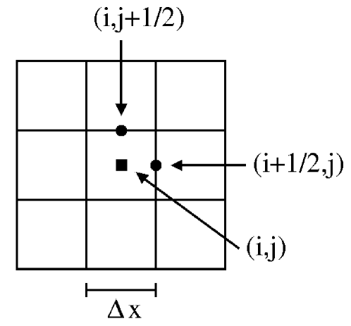
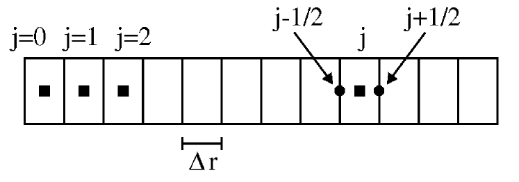
We shall refer to local atmospheric flows in two and three dimensions as problems in “planar” geometry, and full-star flows in three dimensions as problems in “spherical” geometry. The solution in both cases consists of the Cartesian grid solution () and the one-dimensional base state solution (), all of which are cell-centered except for , which is edge-centered. Edge-centered data is denoted by a half-integer subscript. See Figure 1 for a representation of each grid structure. The time step index is denoted as a superscript.
For planar problems, is in alignment with the Cartesian grid unit vector in the outward radial direction, (in two dimensions) or (in three dimensions). We choose so that there will be a simple, direct mapping between the radial array and the Cartesian grid. For spherical problems, is not in alignment with any Cartesian coordinate direction. Our choice of can be independent of ; as in Paper IV, we use . Note that for spherical problems, we place the center of the star at the center of the computational domain, and therefore the center of the star lies at a corner where 8 Cartesian cells meet. See Figure 2 for an illustration of the relationships between the radial array and the Cartesian grid for spherical and planar geometries.


The time-advancement algorithm uses a predictor-corrector formalism. In the predictor step, we compute an estimate of the expansion of the base state, then compute a preliminary estimate of the state at the new time level. In the corrector step, we use this preliminary state to compute a new estimate of the expansion of the base state, and then compute the final state at the new time level. We incorporate reactions and external heating using Strang-splitting. As in previous papers, our algorithm is second-order in space and time.
The full details of the algorithm are presented in Appendix A. The main algorithm description in Appendix A.4 is similar to the description in Paper III, but has been significantly updated to show how we incorporate the time-dependent spherical base state. There are numerous other improvements we have made to the algorithm since papers III and IV, which are described in Appendix A.1. Note that these changes have also been incorporated into the main algorithm description. Overall:
-
•
Appendix A.1 is a summary of algorithmic changes since papers III and IV.
-
•
Appendix A.2 describes how we compute and discretize gravity.
-
•
Appendix A.3 is a description of shorthand notation we use in describing the algorithm.
-
•
Appendix A.4 steps through the algorithm in detail.
-
•
Appendix A.5 describes special treatment given to low density regions in the simulation.
4 Mapping
At many points in the algorithm, we need to map the full state on the Cartesian grid onto a one-dimensional radial array, and vice-versa. Since Paper IV, we have greatly increased the accuracy of the numerical mapping to and from these data structures for spherical problems, most notably the lateral average routine described below. We refer to the procedure for mapping a cell-centered Cartesian field to a cell-centered radial array as a “lateral average”, and we refer to the procedures for mapping an edge- or cell-centered radial array to an edge- or cell-centered Cartesian grid as a “fill”.
4.1 Lateral Average
For any Cartesian cell-centered field, , we define Avg as the lateral average over a layer at constant radius , , as
| (20) |
- planar:
-
This is a straightforward arithmetic average of cells at a particular height since the radial cell centers are in alignment with the Cartesian grid cell centers.
- spherical:
-
It can be shown that any Cartesian cell center is a radius from the center of the star, where is an integer. For example, the Cartesian cell with coordinates relative to the center of the star lies at a distance of from the center of the star, corresponding to . The Cartesian cells with coordinates , or relative to the center of the star also lie at that same distance. For the 3843 resolution examples in this paper, we have verified that a non-zero set of Cartesian cell centers map into each radius until is large enough to correspond to a radius larger than half the width of the computational domain (i.e., the edge of the domain, not the corner of the domain). Figure 3 shows the number of Cartesian cells that map into each radius , which we refer to as the “hit count”, for a 3843 domain. We use this mapping to help construct the lateral average, using the following steps:
-
1.
Create an itemized list, , where each element is associated with a radius from the center of the star.
-
2.
For each , compute the arithmetic average value of the Cartesian cells whose centers lie at the associated radius. As an additional element in the itemized list, include the center of the star (corresponding to a radius of ). Compute this additional value of at this location using quadratic interpolation with , , and a homogeneous Neumann condition at as the stencil points. Note that for very large values of , it is possible that no Cartesian cell centers exist at a radius (i.e., the hit count is zero). If so, we say that has an undefined/invalid value, and we ignore such values for the rest of this procedure.
-
3.
To compute the lateral average, use quadratic interpolation using the value in the itemized list with the closest associated radius, , and the nearest values above and below, and , using divided differences:
where , , and are the three radii associated with , , and . Finally, constrain to lie within the range of , , and so as to not introduce any new maxima or minima.
In §6.1, we show the improvement of this averaging procedure over the Paper IV procedure.
-
1.

4.2 Fill
There are four different mappings from a one-dimensional radial array to the three-dimensional Cartesian grid; below we describe the procedures for planar and spherical geometries separately.
- planar:
-
1.
To map a cell-centered radial array onto Cartesian cell centers, we use direct-injection since the radial cell centers are in alignment with the Cartesian cell centers.
-
2.
To map an edge-centered radial array onto Cartesian cell centers, we average the two nearest radial edge-centered values.
-
3.
To map a cell-centered radial array onto Cartesian edges with normal in the radial direction, we use 4th order spatial interpolation. For example, in two dimensions,
(21) We constrain to lie between the interpolated values, and lower the order of interpolation near domain boundaries. For the Cartesian edges transverse to the base state direction, we use direct-injection since the radial cell centers are in alignment with these Cartesian edges.
-
4.
To map an edge-centered radial array onto Cartesian edges, we use direct-injection on Cartesian edges normal to the base state direction since the radial edges are in alignment with these Cartesian edges. For the remaining Cartesian edges, we average the two nearest radial edge-centered values.
- spherical:
-
1.
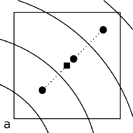
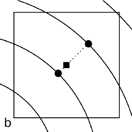
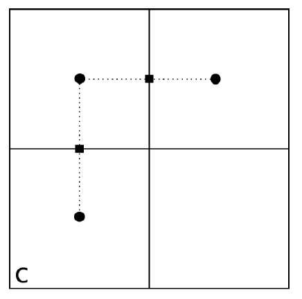
To map a cell-centered radial array onto Cartesian cell centers, we use quadratic interpolation from the nearest three radial cell centers (see Figure 4a). This is a departure from Paper IV, in which we used piecewise constant interpolation.
-
2.
To map an edge-centered radial array onto Cartesian cell centers, we use linear interpolation from the nearest two points (see Figure 4b).
-
3.
To map a cell-centered radial array onto Cartesian edges, we first map the radial array onto Cartesian cell centers (see 1.), then average the two neighboring centers to obtain the Cartesian edge values (see Figure 4c).
-
4.
To map an edge-centered radial array onto Cartesian edges, we first map the radial array onto Cartesian cell centers (see 2.), then average the two neighboring centers to obtain the Cartesian edge values (see Figure 4c).
5 Adaptive Mesh Refinement
Our approach to AMR uses a nested hierarchy of logically rectangular grids with successively finer grids at higher levels. This is based on the strategy introduced for gas dynamics by Berger & Colella (1989), extended to the incompressible Navier-Stokes equations by Almgren et al. (1998), and extended to low Mach number reacting flows by Pember et al. (1998) and Day & Bell (2000). We refer the reader to these works for more details. The key difference between our method and these earlier methods stems from the presence of a one-dimensional base state whose time evolution is coupled to that of the full solution. To the best of our knowledge, there are no existing AMR algorithms for astrophysics or any other field, for flows with a time-dependent base state coupled to the full solution. For simplicity, we present a version of the algorithm with no subcycling in time, i.e., the solution at all levels is advanced with the same time step.
We first summarize our AMR approach without the base state, then discuss how the base state is incorporated in both the planar and spherical cases.
5.1 Creating and Managing the Grid Hierarchy
At each time step the state data is defined on a nested hierarchy of grids, ranging from the base level (), which covers the entire computational domain, to the finest level (). At each level there is a union of non-intersecting rectangular grids with the same spatial resolution. For simplicity, we require that the cells composing the grids be square (), and that the refinement ratio between levels be 2. The grids in the interior of the computational domain are required to be properly nested, i.e., the union of grids at level is completely contained in the union of grids at level . Additionally, in the interior, we require that each grid at level be a distance of at least two level cells from the boundary between level and level grids; this allows us to always fill “ghost cells” at level from the level data (or the physical boundary conditions, if appropriate). We initialize the grid hierarchy and regrid following the procedure outlined in Bell et al. (1994). A user-specified error estimation routine is used to tag cells where more resolution is desired. The tagged cells are grouped into rectangular patches following Berger & Rigoutsos (1991), and subsequently refined to create new grids at next level. Refinement continues until the maximum level is reached.
During Step 0,111The “Step” notation is used in describing the full details of the algorithm in Appendix A.4 grids at all levels are filled directly from the initial data. As the simulation progresses, we periodically check our refinement criteria and regrid as necessary. This regridding takes places during Step 12, before computing the next time step. Newly created grids are filled by using data from previous grids at the same refinement level (if available) or by interpolating from underlying coarser grids.
5.2 Communication between levels
Since we use the same time step to advance the solution at all levels, much of the complication associated with synchronization of data between levels in a subcycling algorithm (see Almgren et al. 1998) is eliminated. The MAC projections in Step 3 and 7 enforce that and respectively, on any coarse edge underlying fine edges are the average of the values on the fine edges. Similarly, the nodal projection in Step 12 enforces that at any coarse node underlying a fine node, the value of on the coarse node is identical to the value on the fine node above it. The additional communication of data between levels occurs as follows:
-
•
Before any explicit operation at level data in ghost cells at that level are filled by interpolating from level , or imposing physical boundary conditions, as appropriate.
-
•
Edge-based fluxes at level that underlie edges at level are defined to be the average of the fluxes on level at that edge. This enforces conservation.
-
•
After any update to the solution, data at finer levels is conservatively averaged onto the underlying coarse grid cells, starting at the finest level.
5.3 AMR with a Time-Dependent Base State
Our specific treatment of AMR is guided by our initial scientific applications, including Type I X-ray bursts and the convective phase of SNe Ia, as well as numerical concerns, most notably the presence of the one-dimensional base state. Our treatment of the base state in an AMR framework differs for planar vs. spherical problems.
For planar problems, our approach is to define a radial base state array with variable mesh spacing. A general localized fine Cartesian grid would require either a base state that exists at multiple resolutions at a particular height, or an interpolation algorithm to obtain the base state value at a particular height if . Both of these methods pose problems, as they generate oscillations in perturbational quantities (such as and the term on the right hand side of the divergence constraint) since the lateral average routine is only defined when the base state is aligned with the Cartesian grid across the width of the domain. Any attempt at interpolation will cause oscillations in the perturbational quantities directly related to the interpolation error. We have found that such oscillations can be detrimental to the results. With these issues in mind, we choose to only allow fine grids to exist that span the width of the domain. This way, the base state exists as a single seamless entity with multiple resolutions depending on height (see Figure 5). We will take advantage of this type of grid structure in our studies of Type I X-ray bursts.


Next, we define ghost cell values for the finer base state levels, and fill these values by interpolating coarser data. This makes the algorithm directly compatible with the one-dimensional time-centered edge state calculation used in Advect Base Density 222The boldface notation refers to numerical modules we have described in Appendix A.3. and Advect Base Enthalpy. In particular, the slopes can be used with a consistent stencil at each level, that is not dependent on the data from any other level once the ghost cells are set.
Finally, whenever we regrid the Cartesian grid data, we regrid the base state to match the grid structure of the Cartesian grid. Then, we set and compute using Enforce HSE. To compute and on the new base state array, we use piecewise linear interpolation of the coarser data to fill any new fine radial cells/edges.
For spherical geometry, we first note that even in the single-level case the radial base state is not aligned with the Cartesian grid. Therefore, we use a base state with a fixed for all levels (see Figure 5). As in the single-level algorithm, we choose , but here, corresponds to resolution of the Cartesian grid at the finest level.
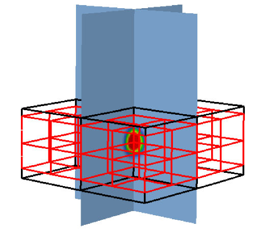
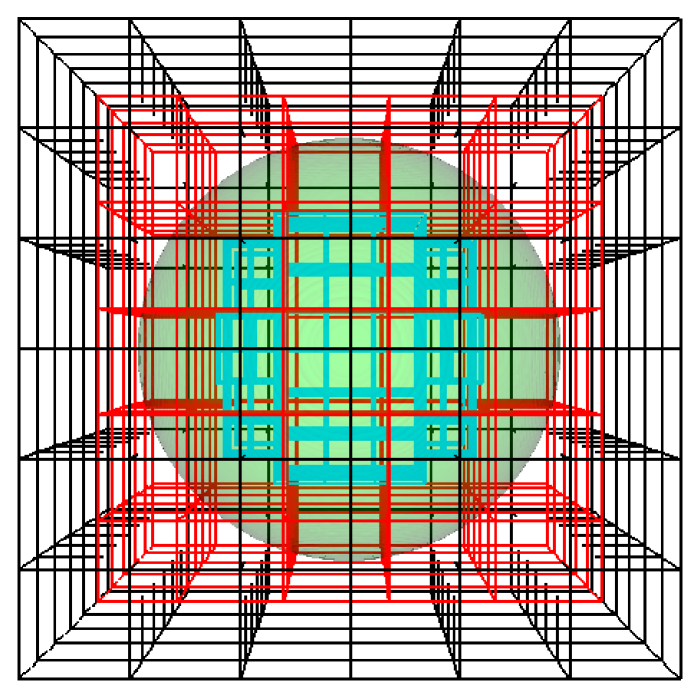
Our next consideration is defining the radial average. First, we first create an itemized list associated with each level of refinement using only Cartesian cells that are not covered by cells at a finer level. At this point one option would be to merge the lists and proceed as in the single-level algorithm; this was tested and found to be problematic. Instead, we choose the list from a chosen particular level and define the average using quadratic interpolation with only this list, as in the single-level case. To decide which list to use, we first examine the three points that would be used by quadratic interpolation at each level. The guiding principle is to avoid using interpolation points with low hit counts. Thus, at each level we find the minimum hit count of the three points; the level which has the largest minimum hit count is the level whose list we use for interpolation. We note that this multi-level average works particularly well when the center of the star is fully refined. This is the case since near the center of the star, there are relatively few Cartesian cells that contribute to each radial bin, so by fully refining the center of the star, we ensure that the multi-level averaging procedure retains the accuracy of a single-level spherical average near the center. For our studies of SNe Ia, we will take advantage of this fact by always refining the center of the star, which is our region of interest (see Figure 12 in §6.6, as an example). In §6.1, we present numerical tests of the new multi-level averaging procedure for spherical geometry.
For both planar and spherical problems, after regridding the Cartesian grid, we make the state thermodynamically consistent by computing (for planar problems) or (for spherical problems). Then, we recompute and as described in Steps 10 and 11.
5.4 Parallel Implementation
We parallelize the algorithm by distributing the grids on each level across processors. Each grid carries a perimeter of ghost cells that are filled from neighboring grids at the same level or interpolated from coarser grids as needed. This allows the data on each grid to be updated independently of the other grids. A typical grid is large enough (e.g., cells) that for explicit operations the cost of computation within each grid greatly exceeds the cost of communication between grids. The linear solves necessary for the MAC projection and approximation nodal projection have higher communication costs, but we still obtain good parallel efficiency for the overall algorithm. A scaling study for MAESTRO can be found in Almgren et al. (2007).
Since the one-dimensional base state arrays are so much smaller than the three-dimensional arrays holding the full solution, each processor owns a copy of the entire one-dimensional base state arrays. Operations such as averaging to define base state quantities require a collection operation among grids, followed by a distribution of the average state to each processor.
6 Test Problems
We have developed a suite of test problems in order to test various aspects of our code.
- •
-
•
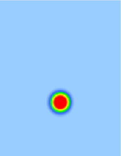
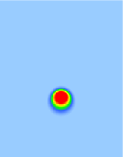
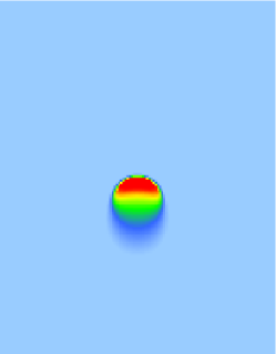
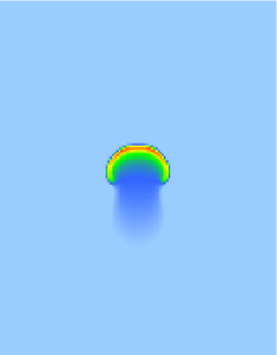
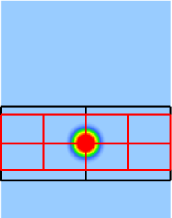
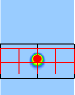
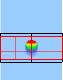
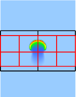
In §6.2, we show that we are able to properly capture the expansion of the base state in a three-dimensional full star simulation due to heating at the center of the star.
-
•
In §6.3, we show that our multi-level algorithm is second-order accurate in space and time by tracking a hot bubble rising in a white-dwarf environment.
-
•
In §6.4, we show that an adaptive algorithm in three-dimensional planar geometry can properly track a hot bubble rising in a white-dwarf environment.
-
•
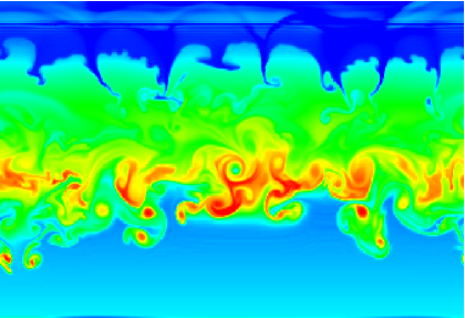
In §6.5, we demonstrate that a multi-level, two-dimensional planar simulation will properly capture the expansion of the base state due to a heating layer, and also that a multi-level simulation is able to capture the same fine-scale structure as a single-level simulation at the same effective resolution over a short time.
-
•
In §6.6, we demonstrate that a full-star simulation with AMR can be used to study the dynamics of convection in white dwarfs.
For test problems §6.2-§6.6, we compute flows in which the density spans at least four orders of magnitude. The large drop in density in the upper atmosphere results in high velocities due to conservation of momentum. This region should not affect the dynamics below the surface in the convecting regions of the star. However, because the time step in the low Mach number code is limited by the highest velocity in the computational domain, the efficiency gains of the low Mach number algorithm are reduced if those velocities persist. We employ a sponging technique to damp such velocities. Damping techniques are commonly used in modeling atmospheric convection (see, for example Durran (1990)). In Paper IV, for full-star convection, we explored the effects of sponging the velocity beginning at two different heights to demonstrate that the dynamics in the upper atmosphere do not affect the convecting regions of the star.
Full details for the sponge implementation can be found in papers III and IV, but in summary, we add a forcing term to the velocity update before the final projection. We use the parameters , and to describe the sponge. The sponge forcing turns on at radius and reaches half of its peak strength at radius . We can control the strength of the forcing with the parameter, . For full-star problems, we also use an outer sponge which prevents the velocities near the domain boundaries from becoming too large.
For all of these tests, we use a publicly available, general stellar equation of state (Fryxell et al., 2000; Timmes & Swesty, 2000), with contributions from ions, radiation, and degenerate/relativistic electrons.
6.1 Mapping
To test the new spherical fill and lateral average routines from §4, we first create a unit cube with resolution and no refinement. We create a radial array with , and initialize the radial array cell centers with the Gaussian profile . We map to Cartesian cell centers with the fill operation, then compute the lateral average of this Cartesian field, . We repeat this process by choosing the grid with two levels of refinement used in the full-star simulation test in §6.6, shown in Figure 12.
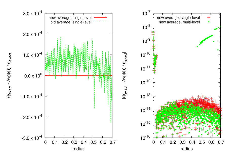
Figure 6 (left) shows the relative error between and ) for the new mapping procedures and the mapping procedures from Paper IV for the single-level test. The new mapping procedure greatly decreases the relative error. Figure 6 (right) is a zoom-in of the relative error for the new mapping. For the single-level grid, the relative error is for and is for . For the test with two levels of refinement, the relative error is for , which is still a vast improvement when compared to the Paper IV mapping applied to a single-level simulation.
6.2 Spherical Base State
To test the base state expansion for spherical geometry, we perform a series of tests similar to those in Paper II which tested the base state expansion in planar problems. We run the same test using three codes— a one-dimensional version of the compressible code, CASTRO (Almgren et al., 2010), in spherical coordinates; a one-dimensional version of MAESTRO in spherical coordinates, and a full three-dimensional spherical star in MAESTRO.
Our initial model is generated by specifying a core density (), temperature ( K), and a uniform composition (, ) and integrating the equation of hydrostatic equilibrium outward while constraining the specific entropy, , to be constant. In discrete form, we solve:
| (22) | |||||
| (23) |
We begin with a guess of and and use the equation of state and Newton-Raphson iterations to find the values that satisfy our system. Since this is a spherical, self-gravitating star, the gravitation acceleration, , is updated each iteration based on the current value of the density. Once the temperature falls below K, we keep the temperature constant, and continue determining the density via hydrostatic equilibrium. This uniquely determines the initial model.
For the one-dimensional simulations, we map the inner cm of the model onto a one-dimensional array with 1280 elements with cm. For the full-star three-dimensional simulation, we map the model onto a cm3 domain with 2563 Cartesian grid cells with cm. For the one and three-dimensional MAESTRO calculations, we use cutoff densities (see Appendix A.5) of and , corresponding to radii of approximately cm and cm, so the star easily fits within the computational domain for each problem. For the full-star three-dimensional simulation, we use an inner sponge with equal to the radius where , equal to the radius where , and s-1. We use the same outer sponge as in Paper IV. All boundary conditions are outflow, except for the center of the one-dimensional simulations, which uses a symmetry boundary condition. We run each simulation using a CFL number of 0.5.
We heat the center of the star for 0.5 seconds and look at the solution at 2.0 seconds (after the compressible solution has had time to re-equilibrate). We use , with chosen to be much larger than the nuclear energy generation rate during the convective phase of SN Ia, in order to see a measurable effect over a few seconds. A comparison of , and at and s for each code is shown in Figure 7. There is excellent agreement between each of the simulations.


6.3 Convergence Test
In Paper III, we demonstrated that our single-level algorithm is second-order in space and time by tracking a hot bubble rising in a white-dwarf environment using two-dimensional planar geometry. Here, we perform the same test to show that our algorithm, with a level of refinement, is second-order in space and time.
We choose a domain size of cm by cm and generate a high resolution initial model with cm (which is equal to for our highest resolution, “exact” solution) using the method described in Appendix C with . For each of the remaining, lower resolution simulations for this test, we generate an initial model using equal to the effective of each simulation by linearly interpolating values from the high resolution model. Next, we add a temperature perturbation of the form:
| (24) |
where cm and is the physical distance between the cell center corresponding to cell and the location cmcm). Then, we call the equation of state to compute a consistent everywhere. We use the reaction network described in § 4.2 in Paper III. We use cutoff densities of , and a sponge with equal to the radius where , equal to the radius where , and s-1. We specify periodic boundary conditions on the side walls, outflow at the top, and a solid wall at the bottom of the domain.
Since we do not have an exact analytical solution, we consider a single-level simulation run with cells and s to be the exact solution. We perform three single-level simulations using resolutions of , and grid cells using fixed time steps of s, s, and s, respectively. We also perform two simulations with a single level of refinement with effective resolutions of and grid cells with fixed time steps of s and s, respectively. These fixed time steps correspond to a CFL of 0.9. We refine all cells in the range cm, so effectively we have refined 1/8th of the domain, making sure the hot spot is contained within the refined region. We run each simulation to s. For this test, whenever we call Enforce HSE to compute from , we use cm as the starting point for integration rather than the location of the cutoff density to ensure that numerical errors due to integrating the equation of hydrostatic equilibrium across simulations with different resolutions are minimized.
In order to compute the error norm for each simulation, we average the data from the exact solution onto a grid with corresponding resolution. We measure the error norm in the physical space corresponding to the refined region using
| (25) |
where is the number of cells we sum over. This form of the error norm gives us the average error per cell. We compute the convergence rate, , between a coarser and finer simulation using
| (26) |
Tables 1 and 2 show the error norms and convergence rates for the single-level and multi-level solutions, respectively. The convergence rates correspond to the two columns on either side of the reported value. We note second order convergence in each variable. Additionally, the magnitude of the error norms for the multi-level simulations is comparable to the corresponding resolution error norms for the single-level simulations. This means that the multi-level simulations are accurately capturing the finer-scale features, as compared to the single-level simulations, i.e., the presence of coarse grid data and/or coarse-fine interfaces is not harming the solution in the refined region.
| Error | Rate, | Error | Rate, | Error | |
|---|---|---|---|---|---|
| 2.02 | 2.30 | ||||
| 2.02 | 2.13 | ||||
| 2.03 | 2.24 | ||||
| 1.97 | 2.09 | ||||
| 2.14 | 2.01 | ||||
| 1.94 | 2.04 |
| Error | Rate, | Error | |
|---|---|---|---|
| 2.25 | |||
| 2.09 | |||
| 2.20 | |||
| 2.08 | |||
| 2.01 | |||
| 2.04 |
6.4 Adaptive Bubble Rise
To test the ability for an adaptive, three-dimensional planar simulation to track a localized feature, we examine a hot bubble rising in a white-dwarf environment. The problem setup is exactly the same as in §6.3, except that we now compute in three dimensions and allow the grid structure to change with time. We choose a domain size of cm by cm cm and for each simulation, we generate an initial model with cm (which is equal to the effective for both of the simulations in this test) using the method described in Appendix C with . We add a temperature perturbation of the form given in equation (24), but in three dimensions with the hot spot centered at location cmcmcm). We will show that the adaptive simulation captures the same dynamics as the single-level simulation in a more computationally efficient manner.
We compute a single-level simulation with grid cells, and an adaptive simulation with two levels of refinement at the same effective resolution. For each cell, if the K, we tag all cells at that height to ensure they are computed at the finest refinement level. We run each simulation to s using a CFL number of 0.9.
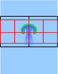
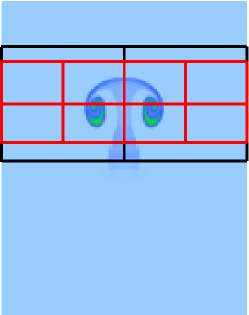
Figure 8 shows the initial profile of and the initial grid structure of the multi-level run. The single-level simulation has 8,388,608 grid cells and takes approximately 32 seconds per time step. The adaptive simulation initially has 131,072 grid cells at the coarsest level, 114,688 cells at the first level of refinement, and 688,128 cells at the finest level of refinement (the number of grid cells at the finer levels changes slightly with time as the grid structure changes to track the bubble) and takes approximately 12 seconds per time step, for a factor of 2.7 speedup. Both computations were performed using 32 processors on the Franklin XT4 machine at NERSC. Figure 9 shows a series of planar slices of the simulations at 0.5 second intervals in order to show that the adaptive simulation captures the same dynamics as the single-level simulation. The vertical distance shown is from to cm.


6.5 Forced Convection
To test the expansion of the base state in a multi-level, two-dimensional planar simulation, we simulate a white-dwarf environment with an external heating layer. We also show that the multi-level simulation captures the same fine-scale structure as a single-level simulation at the same effective resolution for a short time. We performed a similar test in Paper III, but without refinement.
We choose a domain size of cm by cm and for each simulation, we generate an initial model with equal to the effective for that simulation using the method described in Appendix C with cm. The low entropy layer beneath our model atmosphere prevents the convective flow from reaching our lower boundary.
We apply an external heating layer of the form
| (27) |
with cm, erg g-1 s-1, cm, and and being the radial and horizontal physical coordinates of cell . The perturbation parameters are , and . We disable reactions for this test, since the heating layer was chosen to expand the base state over a very short time period, rather than accurately model reactions.
We use cutoff densities of and a sponge with equal to the radius where , equal to the radius where , and s-1. We specify periodic boundary conditions on the side walls, outflow at the top, and a solid wall at the bottom of the domain.
In this test, we use a CFL number of 0.9. We perform two single-level simulations using and cells, and a simulation with two levels of refinement and an effective resolution of cells. For the multi-level simulation, we fix the refined grids, ensuring that cm (which contains the external heating layer) is at the finest level of refinement. We run each simulation to s.
Figure 10 shows , and after 30 seconds of convection for the single-level fine grid simulation and the multi-level simulation. There is an excellent agreement between these two simulations, except in the temperature profiles at the top of the domain. However, this corresponds to a region with density below the cutoff densities where the temperature is extremely sensitive to small density perturbations, and furthermore, is not fully refined in this test, so this is an acceptable difference. Both simulations were performed using 4 processors; the single-level fine grid run required approximately 1.9 seconds per time step and the multi-level run required approximately 0.6 seconds per time step, for a factor of 3 speedup.


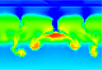
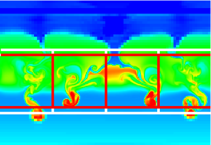
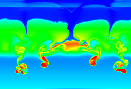
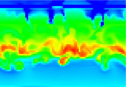
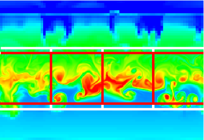
Figure 11 shows the temperature profile after 3 and 4 seconds for each of the three simulations. The vertical distance shown is from cm to cm. At s, the multi-level simulation is able to capture the finer-scale structure visible in the single-level fine grid simulation, which is not captured in the single-level coarse grid simulation. At s, a finer-scale structure is still visible in the multi-level simulation, but the solution begins to drift from the single-level fine grid simulation, which is expected since we are deliberately refining only a part of the convective region.
6.6 Full-Star AMR
We now compute three-dimensional, full-star calculations of convection in a white dwarf. This problem models the convection and energetics of a white dwarf that is a few hours from reaching ignition. We performed similar simulations using an earlier version of the algorithm in Paper IV.
We begin with the one-dimensional white dwarf model described in §2.4 in Paper IV. We map this one-dimensional model into the center of a computational domain of cm on a side. The first simulation is a single-level simulation with 3843 cells. The second simulation is adaptive with two levels of refinement and an effective resolution of 3843 cells. We use the reaction network strategy from Chamulak et al. (2008) to compute the energetics from the carbon burning. This modified network differs from the one used in paper IV in the ash composition (we now burn to an ash with and ) and the energy release (we use a quadratic fit to the -values tabulated on page 164 of Chamulak et al. 2008). Finally instead of destroying two carbon nuclei for each reaction, we use the value of 2.93 describe in that paper. We initialize the simulation with a velocity perturbation described exactly as in §2.4 in Paper IV. We use the same cutoff densities, sponge parameters, and boundary conditions as in §6.2.
Figure 12 shows the initial grid structure of the adaptive simulation. Based on our work in Paper IV, we choose to fully refine all cells where , since at early times, the dynamics of the star are driven by the reactions and convection in this inner region. We wish to examine whether the adaptive simulation can give the same result as the single-level simulation, and the computational efficiency of each simulation.
We use a CFL number of 0.7 and compute to s. We choose two diagnostics used in Paper IV to compare the simulations. Peak temperature is a useful diagnostic since the reaction rates are extremely sensitive to temperature, and thus peak temperature serves as a good guide for observing the progression toward ignition. Peak radial velocity is another useful diagnostic as it is a simple measure of the strength of the convection within the star. Since the solution of our equation is highly non-linear, and the reaction rates scale with temperature as (Woosley et al., 2004), we expect that errors from the coarse grid will perturb the solution at the finest level, eventually causing significant differences in the exact flow field. However, as shown in Paper IV, when we run our simulation to the point of ignition, we require upwards of hundreds of thousands of time steps. Therefore, in the comparison diagnostics in this test, it is sufficient to compare the overall qualitative solution. An exact quantitative comparison is impossible over long times.
Figure 13 shows the evolution of the peak temperature and peak radial velocity over the first 900 s for both simulations. The adaptive simulation gives the same qualitative result as the single-level simulation. As mentioned before, the curves do not match up more closely because the equations are highly non-linear, and slight differences in the solution caused by solver tolerance and discretization error change details of the results, but not the overall qualitative results. The single-level simulation has 56,623,760 grid cells and takes approximately 36 seconds per time step. The adaptive simulation initially has 884,736 grid cells at the coarsest level, 3,511,808 cells at the first level of refinement, and 4,282,048 cells at the finest level of refinement (the number of grid cells at the finer levels changes slightly with time) and takes approximately 18 seconds per time step, for a factor of 2 speedup. Also note that the overall memory requirements are significantly less for the adaptive simulation, as can be seen by the reduced total cell count. Each simulation was run using the Franklin XT4 machine at NERSC with 216 processors.

We note that in the future, when we perform longer calculations up to the point of ignition, we may have to refine a greater portion of the star in order to properly capture the overall dynamics as the convective region expands. In a forthcoming paper, we plan on performing higher resolution studies, where AMR will save us both time and computational resources.
7 Conclusions and Future Work
We have developed a low Mach number hydrodynamics algorithm suitable for full star flows and local atmospheric regions with a time-evolving base state within an AMR framework. In forthcoming papers, we will use MAESTRO to further our scientific investigation of the convective phase of SNe Ia. Our previous simulations in Paper IV were at modest resolution and assumed a constant base state. We are now performing simulations at higher effective resolutions with the use of AMR along with a time-varying base state. As part of this study, we are examining the tagging conditions necessary to model a full-star up to the point of ignition. We are also studying Type I X-ray bursts (Strohmayer & Bildsten, 2006; Lin et al., 2006), which are believed to be caused by the thermonuclear explosive burning of hydrogen and/or helium gas accreted into a thin shell on the surface of neutron stars. We pose this problem in planar geometry, model a small patch of the star, and refine near the base of the accreted layer.
Appendix A Time Advancement Algorithm
A.1 Single-Level Algorithm Changes From Papers III and IV
The single-level algorithm has gone through numerous changes since Papers III and IV. The current single-level algorithm is presented in §A.2–A.5; we summarize here the changes since Papers III and IV:
- •
-
•
For spherical problems, we have improved the accuracy of the mapping of data between the one-dimensional radial array and the three-dimensional Cartesian grid (§4).
-
•
We have upgraded our unsplit piecewise-linear Godunov method for time-centered edge state prediction for the base state and Cartesian grid data to use the unsplit piecewise-parabolic method (PPM) (Colella & Woodward, 1984) with full corner coupling in three dimensions (Miller & Colella, 2002; Saltzman, 1994). We shall refer to this procedure as “computing the time-centered edge states” (§A.3.2, §A.3.4, and Steps 3, 4, 7, 8, and 11 in §A.4).
-
•
As introduced in Paper IV, we update after the call to React State (§A.3.1).
-
•
Rather than evolve using an evolution equation, we simply update using the hydrostatic equilibrium equation (§A.3.3). These two methods are analytically equivalent, but in our experience, the numerical drift associated with evolving using an evolution equation causes the entire solution to drift from thermodynamic equilibrium over time.
-
•
As explained in §2, in the advection step, we predict to edges instead of (Steps 4Hi and 8Hi in §A.4). Thus, a base state enthalpy, is required in order to construct the enthalpy fluxes for the conservative update. Unlike , we do not need to carry the complete evolution of . In practice, we set equal to the lateral average of the full state enthalpy after the first call to React State, i.e., . We then advect without reactions or heating to mirror the treatment of in the advection step (Steps 4G and 8G in §A.4).
-
•
In the advection step, rather than simultaneously updating each of the base state quantities, followed by an update of all the full state quantities, we have interwoven these updates in order to obtain better accuracy. In order: we advect , advect , correct , advance , advect , and advect (Steps 4 and 8 in §A.4). This enables us to use a time-centered rather than a time-lagged for the enthalpy update.
-
•
Rather than compute and use it to adjust to account for convecting overturning, as was done in Correct Base in Paper III, we simply use the lateral average operator to enforce , which is simpler and analytically equivalent (Steps 4D and 8D in §A.4). We use the improved averaging procedure described in §4.1, which greatly improves the accuracy of this mapping for spherical problems.
- •
-
•
For planar problems, we evolve the enthalpy for the sole purpose of updating the temperature, which is subsequently fed into the reaction network and used in computing thermodynamic derivatives. For spherical problems, as described in Paper IV, we instead define from ,, and . This completely decouples the enthalpy from the rest of the solution. Our experience has shown that, with spherical geometry, the discretization errors are minimized by using the hydrostatic, radial base state pressure to define temperature. We still evolve the enthalpy, but we use it as a diagnostic to examine to what extent our numerical method keeps the solution in thermodynamic equilibrium.
A.2 Gravity
For planar problems, we treat gravity as constant in space and time. For spherical problems, gravity is computed directly from in the following manner. First, we define the enclosed mass at radial edges and cell centers:
| (A1) |
In practice, we compute as , in order to minimize roundoff error at large radii and use a similar formula for the radial difference term in the equation for . Next, we define the gravity at both radial edges and cell centers:
| (A2) |
We indicate which base state density is used to compute gravity by using a shorthand notation with superscripts on , e.g., .
A.3 Main Algorithm Notation
We make use of the following shorthand notations in outlining the algorithm:
A.3.1 Reactions
React State evolves the species and enthalpy due to reactions through according to:
| (A3) |
Full details of the solution procedure can be found in Paper III. We then define:
| (A4) | |||||
| (A5) |
where the enthalpy update includes external heat sources . As introduced in Paper IV, we update the temperature using for planar geometry or for spherical geometry. Note that the density remains unchanged within React State, i.e., .
A.3.2 Advection
Advect Base Density is the process by which we update the base state density through in time. We keep the time-centered edge states, , since they are used later in discretization of for planar problems.
- planar:
- spherical:
-
The base state density update now includes the area factors in the divergences:
(A8) In order to compute the time-centered edge states, an additional geometric term is added to the forcing, due to the spherical discretization of (14):
(A9)
A.3.3 Update
Enforce HSE has replaced Advect Base Pressure from Paper III as the process by which we update the base state pressure. Rather than discretizing the evolution equation for , we enforce hydrostatic equilibrium directly, which is numerically simpler and analytically equivalent. We first set and then update using:
| (A10) |
where . As soon as , we set for all remaining values of . Then we compare with and offset every element in so that . We are effectively using the location where the drops below as the starting point for integration.
A.3.4 Advection
Advect Base Enthalpy is the process by which we update the base state enthalpy through in time.
- planar:
- spherical:
-
The base state enthalpy update now includes the area factors in the divergences:
In order to compute the time-centered edge states, an additional geometric term is added to the forcing, due to the spherical discretization of (15):
(A14)
A.3.5 Computing
Here we describe the process by which we compute . The arguments are different for planar and spherical geometries.
-
Compute Planar :
In Paper III, we showed that for planar geometries, and derived an alternate expression for equation (11). We compute using equation (35) in Paper III using the following discretization:
(A15) with .
-
Compute Spherical :
A.4 Main Algorithm Description
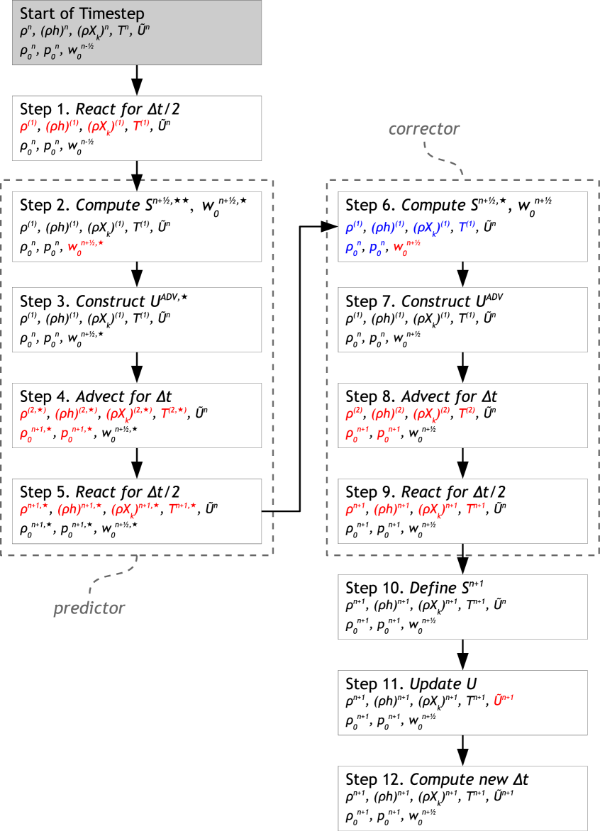
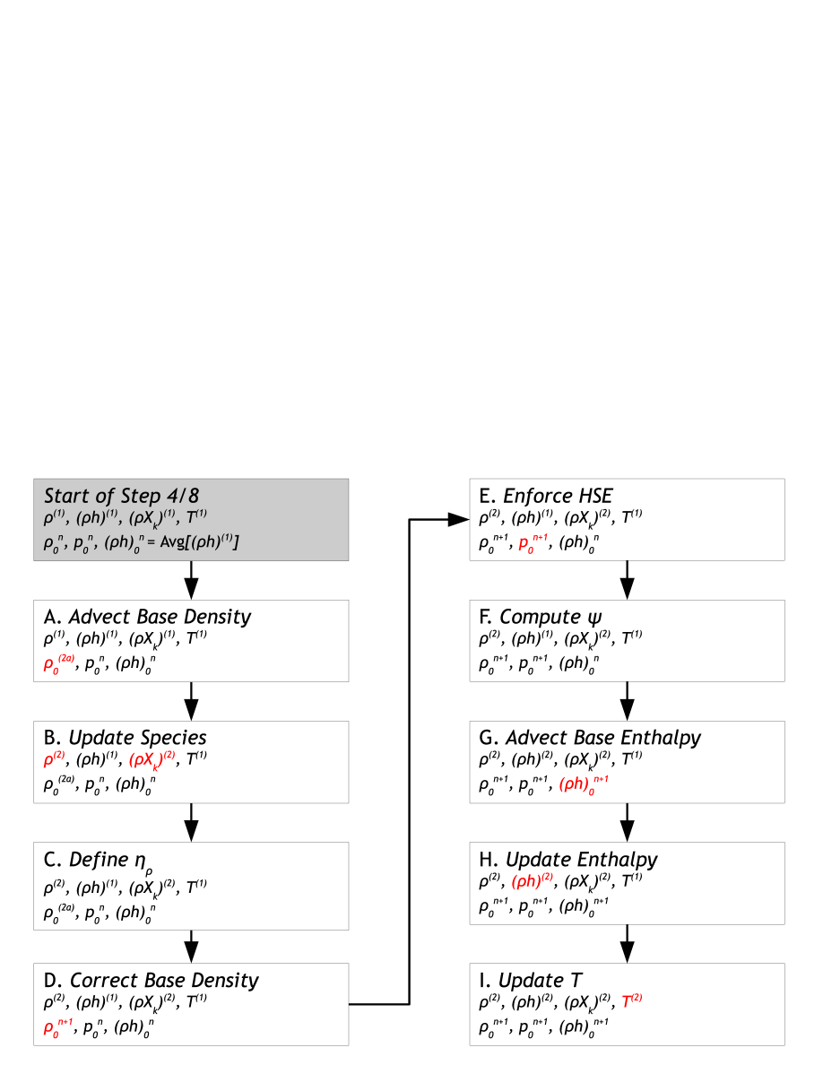
We now describe the main algorithm, making frequent use of the shorthand developed above. In summary, in the predictor step (Steps 2-5) we use an estimate of the expansion term, , to compute a preliminary solution at the new time level, denoted with an “” superscript. In the corrector step (Steps 6-9), we use the results from the predictor step to compute a more accurate expansion term, and compute the final solution at the new time level, denoted with an “” superscript. We use Strang-splitting to achieve second-order accuracy in time. See Figure 14 for a flow chart of the algorithm, including the notation used as we advance the solution by Figure 15 is a flow chart of the advection steps (Steps 4 and 8), which includes the notation we use as we advect the solution through a time interval of .
The discussion that follows mirrors closely that in Paper III, but has been updated to reflect all the changes throughout the algorithm. The advance of the state through a single time step appears as:
- Step 0.
-
Initialization
This step remains unchanged from Paper III. The initialization step only occurs at the beginning of the simulation. The initial values for , and are specified from the problem-dependent initial conditions. The initial time step, , is computed as in Paper III. Finally, initial values for , and come from a preliminary pass through the algorithm.
- Step 1.
-
React the full state through the first time interval of
Call React State
. - Step 2.
-
Compute the provisional time-centered expansion, , provisional base state velocity, , and provisional base state velocity forcing.
-
A.
Compute . We compute an estimate for the time-centered expansion term in the velocity divergence constraint (eq. [12]). For the first time step (), we set
(A19) where is found during initialization. For other time steps , following Bell et al. (2004), we extrapolate to the half-time using at the previous and current time levels
(A20) Next, compute
(A21) -
B.
Compute .
-
For planar geometry, call
Compute Planar. -
For spherical geometry, call
Compute Spherical.
-
-
C.
Compute the provisional base state velocity forcing. Rearrange equation (9),
(A22) with the following discretization:
(A23) where and are defined as
(A24) If , we use .
-
A.
- Step 3.
-
Construct the provisional time-centered advective velocity on edges, .
Using equation (10), we compute time-centered edge velocities, , using . The superscript refers to the fact that the predicted velocity field does not satisfy the divergence constraint. We then construct from using a MAC projection, as described in detail in Appendix B of Paper III. We note that satisfies the discrete version of as well as
(A26) (A27) where is computed as described in Appendix C of Paper III.
- Step 4.
-
Advect the base state and full state through a time interval of
-
A.
Update , saving the time-centered density at radial edges by calling
Advect Base Density.
-
B.
Update using a discretized version of equation (1) omitting the reaction terms, which were already accounted for in React State. The update consists of two steps:
-
i.
Compute the time-centered species edge states, , for the conservative update of . We use equations (17) and (13) to predict and to time-centered edges using , yielding and . We convert the perturbational density full state density using
(A28) where the base state density terms are mapped to Cartesian edges. Then,
. -
ii.
Evolve using
(A30)
-
i.
-
C.
Define a radial edge-centered .
-
For planar geometry, since ,
(A31) -
For spherical geometry, first construct on Cartesian cell centers using:
(A32) Then,
(A33) This gives a radial cell-centered . To get at radial edges, average the two neighboring radial cell-centered values.
-
-
D.
Correct by setting Avg.
-
E.
Update by calling Enforce HSE.
-
F.
Compute .
-
For planar geometry,
(A34)
-
-
G.
Update . First, compute Avg. Then, call
Advect Base Enthalpy. -
H.
Update the enthalpy using a discretized version of equation (3), again omitting the reaction and heating terms since we already accounted for them in React State. This equation takes the form:
(A38) For spherical geometry, we solve the analytically equivalent form,
(A39) which experience has shown to minimize the drift from thermodynamic equilibrium. The update consists of two steps:
-
i.
Compute the time-centered enthalpy edge state, for the conservative update of . We use equation (18) to predict to time-centered edges, using , yielding . We convert the perturbational enthalpy to a full state enthalpy using
(A40) For planar geometry, we map directly to Cartesian edges. In spherical geometry, our experience has shown that a slightly different approach leads to reduced discretization errors. We first map and to Cartesian edges separately, and then multiply these terms to get .
-
ii.
Evolve .
-
For planar geometry,
(A41) -
For spherical geometry,
(A42)
-
Then, for each Cartesian cell where , we recompute enthalpy using
(A43) -
i.
-
I.
Update the temperature using the equation of state: (planar geometry) or (spherical geometry).
-
A.
- Step 5.
-
React the full state through a second time interval of
Call React State
- Step 6.
-
Compute the time-centered expansion, , base state velocity, , and base state velocity forcing.
-
A.
Compute . First, compute with
(A44) where and the thermodynamic quantities are defined using and as inputs to the equation of state. Then, define
(A45) -
B.
Compute . First, define
(A46) with
(A47) -
For planar geometry, call
Compute Planar. -
For spherical geometry, call
Compute Spherical
.
-
-
C.
Compute the base state velocity forcing. Rearrange equation (A22),
(A48) where and are defined as
(A49) If , we use .
-
A.
- Step 7.
-
Construct the time-centered advective velocity on edges, .
The procedure to construct is identical to the procedure for computing in Step 3, but uses the updated values and rather than and . We note that satisfies the discrete version of as well as
(A51) (A52) - Step 8.
-
Advect the base state and full state through a time interval of
-
A.
Update , saving the time-centered density at radial edges by calling
Advect Base Density.
-
B.
Update . This step is identical to Step 4B except we use the updated values , and rather than , and . In particular:
-
C.
Define a radial edge-centered .
-
For planar geometry,
(A56) -
For spherical geometry, first construct on Cartesian cell centers using:
(A57) Then,
(A58) This gives a radial cell-centered . To get at radial edges, average the two neighboring cell-centered values.
-
-
D.
Correct by setting Avg.
-
E.
Update by calling Enforce HSE.
-
F.
Compute .
-
For planar geometry,
(A59)
-
-
G.
Update by calling Advect Base Enthalpy.
-
H.
Update the enthalpy. This step is identical to Step 4H except we use the updated values , and rather than
, and . In particular:-
i.
Compute the time-centered enthalpy edge state, for the conservative update of . We use equation (18) to predict to time-centered edges with , yielding . We convert the perturbational enthalpy to a full state enthalpy using
(A62) -
ii.
Evolve .
-
For planar geometry,
(A63) -
For spherical geometry,
where is defined as .
-
Then, for each Cartesian cell where , we recompute enthalpy using
(A65) -
i.
-
I.
Update the temperature using the equation of state: (planar geometry) or (spherical geometry).
-
A.
- Step 9.
-
React the full state through a second time interval of
Call React State
- Step 10.
-
Define the new time expansion, , and .
-
A.
Define
(A66) where and the thermodynamic quantities are defined using , , and as inputs to the equation of state. Then, compute
(A67) -
B.
Define
(A68)
-
A.
- Step 11.
-
Update the velocity.
First, we compute the time-centered edge velocities, . Then, we define
(A69) We update the velocity field to by discretizing equation (10) as
where approximates a cell-centered gradient from nodal data. Again, the superscript refers to the fact that the updated velocity does not satisfy the divergence constraint.
Finally, we use an approximate nodal projection to define from such that approximately satisfies
(A71) where is defined as
(A72) As part of the projection we also define the new-time perturbational pressure, This projection necessarily differs from the MAC projection used in Step 3 and Step 7 because the velocities in those steps are defined on edges and is defined at cell centers, requiring different divergence and gradient operators. Details of the approximate projection are given in Paper III.
- Step 12.
-
Compute a new
Compute for the next time step with the procedure described in §3.4 of Paper III using as computed in Step 6 and as computed in Step 11.
This completes one step of the algorithm.
Figure 14 is a flow chart summarizing the 12 step algorithm, including the notation used as we advance the solution by Figure 15 is a flow chart of the advection steps (Steps 4 and 8), which includes the notation we use as we advect the solution through a time interval of .
A.5 Numerical Cutoffs
As discussed in Paper IV, in order to prevent the velocity from becoming too large in low density regions far from the center of the star, we impose a cutoff at a moderately small density, , and hold the density at this constant value outside of the star. The cutoff affects the evolution in the following ways:
-
•
After advancing enthalpy in the advection step (Steps 4Hii and 8Hii in §A.4), we recompute the enthalpy using the equation of state if .
-
•
When computing gravity (§A.2) we only add to if in order to prevent an unphysical amount of mass from contributing to the calculation.
-
•
When computing in Enforce HSE (§A.3.3), we hold constant once .
-
•
In React State (§A.3.1), we set and if .
-
•
When computing , (Steps 4F and 8F in §A.4) we set if .
-
•
When we compute the velocity forcing in Steps 3, 7, 11, and 12, we set the buoyancy term (the term proportional to ) to zero if .
Additionally, we use an anelastic cutoff density, , in the computation of (Steps 3, 7, and 11 in §A.4). When , we set .
Appendix B Computing for spherical problems
Recall that we want to solve
| (B1) |
for the base state velocity, We first decompose by setting , where the term is the contribution to due to the expansion term:
| (B2) |
Then we can write an equation for the remaining term, :
| (B3) |
Multiplying equation (B3) through by , taking another derivative with respect to , and switching the order of temporal and spatial derivatives, we get:
| (B4) |
To solve for we will need to substitute for the derivatives of To do so we start with the hydrostatic equilibrium equation,
| (B5) |
where is the mass enclosed at radius and is the gravitational constant. Using this, we can then write equation (B4) as:
| (B6) | |||||
The mass enclosed inside any radius, , is , or alternately, . The Lagrangian derivative of the enclosed mass is then:
| (B7) | |||||
where we used the spherical form of equation (29) in Paper III,
| (B8) |
to eliminate . We note that in the absence of any mixing, , and . Equation (B7) allows us to write the Lagrangian change in the gravitational acceleration as:
| (B9) | |||||
Putting it all together, equation (B6) becomes:
| (B10) |
Finally, we can use equation (B8) to write equation (B10) as:
| (B11) | |||||
We discretize this elliptic equation in the radial dimension as:
| (B12) | |||||
where we choose to solve for rather than so that we can easily enforce at the the upper boundary. Then, using hydrostatic equilibrium, we expand this to
| (B13) |
If we write this in matrix form, so that:
| (B14) |
then:
| (B15) | |||||
| (B16) | |||||
| (B17) | |||||
| (B18) | |||||
We define the lower boundary condition, at , which corresponds to by setting:
| (B19) |
We also specify at the the upper boundary, which corresponds to the location where falls below , by setting:
| (B20) |
Finally, . Once falls below , we hold constant.
Appendix C Test Problem Initial Model
We use the same general initial model for the convergence test (§6.3), adaptive bubble rise test (§6.4) and forced convection test (§6.5). We define a base temperature, K, and density, , at some height above the bottom of the domain ( varies in each problem, and can be equal to zero). This defines a base entropy, . The gravitational acceleration, , is constant. The composition is uniform everywhere with and . For , we integrate the equation of hydrostatic equilibrium along with the constraint that entropy is constant:
| (C1) | |||||
| (C2) |
upwards from . We define a temperature cutoff, K, and when , we replace equation (C2) with . If we choose , then we must also define the model for . In this case, we define a desired linear entropy profile with a discontinuous jump from as
| (C3) |
This entropy profile creates a convectively stable layer below the atmosphere to prevent any motions generated from heating above from interfering with the lower boundary. The initial model for this region is then computed by integrating:
| (C4) | |||||
| (C5) |
downward from .
References
- Almgren et al. (2010) Almgren, A. S. et al. 2010, accepted for publication in ApJS
- Almgren et al. (1998) Almgren, A. S., Bell, J. B., Colella, P., Howell, L. H., & Welcome, M. 1998, Journal of Computational Physics, 142, 1
- Almgren et al. (2008) Almgren, A. S., Bell, J. B., Nonaka, A., & Zingale, M. 2008, Astrophysical Journal, 684, 449
- Almgren et al. (2006a) Almgren, A. S., Bell, J. B., Rendleman, C. A., & Zingale, M. 2006a, Astrophysical Journal, 637, 922
- Almgren et al. (2006b) —. 2006b, Astrophysical Journal, 649, 927
- Almgren et al. (2007) Almgren, A. S., Bell, J. B., & Zingale, M. 2007, Journal of Physics Conference Series, 78, 2085
- Bell et al. (1994) Bell, J. B., Berger, M. J., Saltzman, J. S., & Welcome, M. 1994, SIAM J. Sci. Statist. Comput., 15, 127
- Bell et al. (2004) Bell, J. B., Day, M. S., Rendleman, C. A., Woosley, S. E., & Zingale, M. A. 2004, Journal of Computational Physics, 195, 677
- Berger & Colella (1989) Berger, M. J., & Colella, P. 1989, Journal of Computational Physics, 82, 64
- Berger & Rigoutsos (1991) Berger, M. J., & Rigoutsos, J. 1991, IEEESMC, 21, 1278
- Chamulak et al. (2008) Chamulak, D. A., Brown, E. F., Timmes, F. X., & Dupczak, K. 2008, Astrophysical Journal, 677, 160
- Colella & Woodward (1984) Colella, P., & Woodward, P. R. 1984, Journal of Computational Physics, 54, 174
- Day & Bell (2000) Day, M. S., & Bell, J. B. 2000, Combust. Theory Modelling, 4, 535
- Durran (1990) Durran, D. 1990, Meteorol. Monographs, 23, 59
- Fryxell et al. (2000) Fryxell, B. et al. 2000, Astrophysical Journal Supplement, 131, 273
- Glasner et al. (2007) Glasner, S. A., Livne, E., & Truran, J. W. 2007, Astrophysical Journal, 665, 1321
- Höflich & Stein (2002) Höflich, P., & Stein, J. 2002, Astrophysical Journal, 568, 779
- Kuhlen et al. (2006) Kuhlen, M., Woosley, S. E., & Glatzmaier, G. A. 2006, Astrophysical Journal, 640, 407
- Lin et al. (2006) Lin, D. J., Bayliss, A., & Taam, R. E. 2006, Astrophysical Journal, 653, 545
- Meakin & Arnett (2007) Meakin, C. A., & Arnett, D. 2007, Astrophysical Journal, 665, 690
- Miller & Colella (2002) Miller, G. H., & Colella, P. 2002, Journal of Computational Physics, 183, 26
- Pember et al. (1998) Pember, R. B., Howell, L. H., Bell, J. B., Colella, P., Crutchfield, W. Y., Fiveland, W. A., & Jessee, J. P. 1998, Comb. Sci. Tech., 140, 123
- Saltzman (1994) Saltzman, J. 1994, Journal of Computational Physics, 115, 153
- Strohmayer & Bildsten (2006) Strohmayer, T., & Bildsten, L. 2006, Compact Stellar X-Ray Sources, ed. W. H. G. Lewin & M. van der Klis (Cambridge: Cambridge Univ. Press), 113–+
- Timmes & Swesty (2000) Timmes, F. X., & Swesty, F. D. 2000, Astrophysical Journal Supplement, 126, 501
- Woosley et al. (2004) Woosley, S. E., Wunsch, S., & Kuhlen, M. 2004, Astrophysical Journal, 607, 921
- Zingale et al. (2009) Zingale, M., Almgren, A. S., Bell, J. B., Nonaka, A., & Woosley, S. E. 2009, Astrophysical Journal, 704, 196