Magnetic Braking and Damping of Differential Rotation in Massive Stars
Abstract
Fragmentation of highly differentially rotating massive stars that undergo collapse has been suggested as a possible channel for binary black hole formation. Such a scenario could explain the formation of the new population of massive black holes detected by the LIGO/VIRGO gravitational wave laser interferometers. We probe that scenario by performing general relativistic magnetohydrodynamic simulations of differentially rotating massive stars supported by thermal radiation pressure plus a gas pressure perturbation. The stars are initially threaded by a dynamically weak, poloidal magnetic field confined to the stellar interior. We find that magnetic braking and turbulent viscous damping via magnetic winding and the magnetorotational instability in the bulk of the star redistribute angular momentum, damp differential rotation and induce the formation of a massive and nearly uniformly rotating inner core surrounded by a Keplerian envelope. The core + disk configuration evolves on a secular timescale and remains in quasi-stationary equilibrium until the termination of our simulations. Our results suggest that the high degree of differential rotation required for seed density perturbations to trigger gas fragmentation and binary black hole formation is likely to be suppressed during the normal lifetime of the star prior to evolving to the point of dynamical instability to collapse. Other cataclysmic events, such as stellar mergers leading to collapse, may therefore be necessary to reestablish sufficient differential rotation and density perturbations to drive nonaxisymmetric modes leading to binary black hole formation.
pacs:
04.25.D-, 47.75.+f, 97.60.-s, 95.30.QdI Introduction
The multiple detections by the LIGO/VIRGO Scientific Collaboration (LVSC) of gravitational wave (GW) signals produced by binary black hole (BH) mergers Abbott et al. (2016a); Abbott et al. (2016b, 2017a, 2017b, 2017, 2018) provides the clearest evidence of the existence and common occurrence of close binary BHs. These detections also point to a new population of stellar-mass binary BHs whose masses are larger than those of the twenty X-ray BH binaries with masses Remillard and McClintock (2006), and it raises a puzzle regarding the origin of these massive BH binaries.
There are various scenarios proposed to explain the formation of massive BH binaries, such as the coalescence of primordial black holes Bird et al. (2016); Carr et al. (2016); Clesse and Garcí a-Bellido (2017); Eroshenko (2018) and failed supernova explosion Schrøder et al. (2018). The collapse of a massive star () has been suggested as one of the most plausible formation channels for BHs observed by the LVSC Tutukov and YungelSon (1993); Voss and Tauris (2003); Schrøder et al. (2018). As the final mass of the BH remnant depends sensitively on the mass and metallicity of the progenitor stars Woosley et al. (2002), it is somehow expected that the direct–collapse of Population III (Pop III) stars form the most massive BHs Belczynski et al. (2010); Dominik et al. (2013). This hypothesis was confirmed by population synthesis simulations of Pop III stars Kinugawa et al. (2014), where binary BHs with typical mass of were formed from Pop III binary evolutions with masses ranging between to . The study in Belczynski et al. (2016) suggests that a binary containing massive stars with masses and at redshift may be the progenitor of the first BH binary detected by the LVSC (event GW150914) Abbott et al. (2016a). Later, it was shown in Stevenson et al. (2013) that the events GW150914 and GW151226, as well as the lower-confidence event LVT151012, may be explained by the isolated binary evolution channel (i.e. assuming that the binary never interacts with another star) from progenitor stellar binaries with masses between . This channel involves the formation of a common envelope through which mass is transferred between the secondary star and its companion via stellar winds. However, such a common-envelope phase is not well understood and results in great physical uncertainties for the BH formation rate due to the lack of observational evidence Kalogera et al. (2004). To avoid this phase, an evolution channel including massive overcontact binaries, where two tightly bound stars are sufficiently mixed due to their tidally induced high spin, has been considered Marchant et al. (2016). Prior to collapse, the massive close binary components are fully mixed and achieve chemical homogeneity. As the hydrogen burning ends nearly simultaneously for the two binary components, the post-main-sequence expansion is suppressed due to the absence of a hydrogen-rich envelope. According to the mass exchange mechanism, this evolution route is therefore likely to produce BH binaries with a large mass ratio, as in GW150914 de Mink and Mandel (2016). Recently, a highly spinning and aligned BHBH event in the first observing run (O1) of Advanced LIGO Abbott et al. (2018) was recently reported Zackay et al. (2019), which lends support to the hypothesis that stellar binaries may be the progenitors of at least some LVSC BHBHs.
It also has been suggested that stellar-massive BHs can be formed via dynamical interactions in dense clusters. In clusters with low metallicities, such as the cores of globular clusters (GCs) or dense AGNs 111However, low-metallicity AGN is extremely rare from observations. For details, see, e.g., http://dx.doi.org/10.1111/j.1365-2966.2006.10812.x. it is possible to form binary systems dynamically via gravitational interactions among a population of stellar-mass BHs Rodriguez et al. (2016a); Chatterjee et al. (2017) or hierarchical mergers of smaller BHs Fishbach et al. (2017). In particular, a simulation of GCs of mass with many-body dynamics and stellar evolution has provided an evolutionary channel for BH binaries similar to GW150914 Rodriguez et al. (2016b). It is expected that the two mechanisms described above can be distinguished by the binary spins from a large, future sample of BH mergers. The BH binaries formed from direct collapse of massive stars are more likely to result in aligned spins due to tidal interactions and/or mass transfer, while dynamically formed binaries will have randomly oriented spins. In addition, the further merging of the massive BH remnants in GCs may finally form more massive intermediate-mass black holes (IMBHs), defined as BHs with mass Miller and Colbert (2004). An all-sky survey of GW signals from binary IMBHs has been performed by LVSC. For such systems, the merger rate is constrained to be in the local Universe with confidence Abbott et al. (2017). Other evolution channels, such as the direct collapse of very massive Pop III stars, can also form IMBHs Miller and Colbert (2004); Gair et al. (2011).
Among the binary BH detections by LVSC, GW150914 and GW170104 are possibly associated with electromagnetic (EM) counterparts Connaughton et al. (2016); Verrecchia et al. (2017). Although the EM emission is unexpected for binary BHs mergers in pure vacuum (see e.g. Lyutikov (2016)), in these two events, gamma-ray signals with isotropic energy have been observed shortly after the peak GW signals Connaughton et al. (2016); Verrecchia et al. (2017). With the assumption that the EM transient is connected to the GW events, fully general relativistic magnetohydrodynamic (GRMHD) simulations in Khan et al. (2018) show that magnetized disk accretion onto a BH binary could explain GW and EM counterparts such as the GBM hard X-ray signal reported 0.4s after GW150914. Massive star fragmentation during gravitational collapse has been proposed as an alternative scenario Loeb (2016). However, numerical simulations and analytic studies have shown that binary BHs coalescence within a dense stellar gas () produces a waveform different from one in vacuum due to gas drag Fedrow et al. (2017); Dai et al. (2017). To rectify this effect, the single-progenitor scenario with an accretion rate times the Eddington rate prior to merger has been suggested D’Orazio and Loeb (2018). This so-called giga-Eddington accretion can drive out the stellar gas as well as alter the time delay between GW and EM signals. However, that scenario may not account for all the physical processes involved, in particular magnetically-driven processes (see e.g. Gold et al. (2014, 2014); Khan et al. (2018)), which can have a dynamical impact on the evolution channel.
| Case | ||||||||
|---|---|---|---|---|---|---|---|---|
| N29 | 2.9 | 4.139 | 161 | 36.92 | 0.091 | |||
| N295 | 2.95 | 4.801 | 192 | 52.44 | 0.085 |
(a) where .
(b) .
(c) .
(d) .
Returning to the collapse of massive stars as the origin of massive BHs and massive BH binaries, we note that massive stars are radiation dominated and well-approximated by an () polytrope. During their evolution, very massive (and supermassive) stars cool and contract until they ultimately encounter a relativistic, dynamical instability leading to catastrophic collapse to BHs (see Baumgarte and Shapiro (1999); Shibata and Shapiro (2002); Saijo et al. (2002); Zink et al. (2006); Saijo and Hawke (2009); Shibata et al. (2016); Butler et al. (2018)). Massive stars that are uniformly rotating remain nearly axisymmetric during the collapse, as shown by post-Newtonian Saijo et al. (2002) and fully general relativistic (GR) simulations Sun et al. (2017, 2018). However, massive stars that are differentially rotating with a sufficiently high ratio of rotational kinetic energy to gravitational potential energy () are secularly unstable to forming bar modes during the course of their evolution Bodenheimer and Ostriker (1973); New and Shapiro (2001a, b). In addition, differentially rotating massive stars with nonaxisymmetric (e.g. bar mode) density perturbations and undergoing collapse can fragment into self-gravitating, collapsing components that form seed BHs Zink et al. (2006, 2007). In some cases, this fragmentation may lead to the formation of massive BH binaries Reisswig et al. (2013).
Even though intensive studies of the evolution channels and the interactions of collapsing massive stars have been studied previously, our understanding of the role of the magnetically–driven instabilities during their stellar evolution prior to collapse remains poor.
Newtonian simulations of magnetic braking (i.e. winding) and viscous damping of an incompressible, differentially rotating infinite cylinder model were performed in Shapiro (2000). It was found that differential rotation could generate toroidal Alfvén waves that convert an appreciable fraction of rotational kinetic energy to magnetic energy and drive the star toward uniform rotation (“magnetic braking”). The destruction of differential rotation was also demonstrated later on in a compressible cylinder model Cook et al. (2003) and in relativistic, neutron star models, both incompressible Liu and Shapiro (2004) and compressible Etienne et al. (2006). The role of turbulent viscosity in damping differential rotation in rapidly spinning, neutron stars obeying a “stiff” () equation of state (EOS) was demonstrated by simulations in axisymmetry in Duez et al. (2004), where the Navier-Stokes equations with a shear viscosity were solved in full GR. They found that the viscosity drives the neutron stars to a high density, uniformly rotating core surrounded by a Keplerian disk in which the core could either collapse to a BH or remain stable depending on its mass and the viscous build-up of thermal pressure. Subsequently, the role of magnetic fields in driving viscous turbulence via the magneto-rotational instability (MRI), which damps the differential rotation in a hypermassive neutron star, was demonstrated by GRMHD simulations in axisymmetry in Duez et al. (2006a, b); Shibata et al. (2006); Etienne et al. (2006). They showed that the magnetic energy is amplified both by the winding of field lines and MRI, and that the differential rotation is significantly reduced due to the magnetic braking and MRI-induced turbulent viscous damping.
In this paper, we explore this braking and damping scenario in weakly magnetized, differentially rotating massive stars in hydrostatic equilibrium. In particular, we perform GRMHD simulations to probe the effects of magnetic winding and magnetic-induced turbulent viscosity that can break the differential rotation in massive stars. We consider massive stars governed by a soft () EOS. We first show that, for magnetized stars with characteristic masses greater than several hundred , the hierarchy of physical timescales meets the criteria for the magnetic damping of differential rotation within stellar lifetimes. Then we construct stable equilibrium stars with the same differentially rotating profiles as in the initial (collapsing) configurations employed in Reisswig et al. (2013), where fragmentation of seed density perturbations into BH binaries occurs. We endow the stars with a dynamically weak, dipole magnetic field confined to the stellar interior and evolve the resulting magnetized equilibrium configuration in 3+1 dimensions using our Illinois GRMHD code. We find that well prior to collapse, magnetic braking and turbulent viscosity induces the formation of an inner core surrounded by a thick, Keplerian, circumstellar disk after several Alfvén timescales. As anticipated, magnetic braking, induced by the toroidal winding of the magnetic field, and viscous damping, induced by magnetic turbulence triggered by the MRI, drive the inner core to uniform rotation. The new-born core + disk configuration evolves on a secular (viscous) timescale and remains in quasistationary equilibrium until we terminate the simulations. Our results suggest that a stellar fragmentation scenario for a massive star that evolves in isolation is not a plausible formation channel for binary BHs. Other cataclysmic events, such as the merger of two massive stars, may be necessary to re-establish sufficient differential rotation to drive nonaxisymmetric modes leading to fragmentation of a dynamically unstable remnant into binaries during collapse. Our results apply for stars prior to BH formation with characteristic masses greater than several hundred solar masses. The masses in our simulations are chosen for demonstration purposes and were selected for their microphysical simplicity and computational practicality. However, we do expect qualitative similar outcomes to apply for lower masses relevant to the LIGO/Virgo BH progenitors.
The structure of the remainder of the paper is as follows. In Sec. II, we calculate several key physical timescales and show that the hierarchy of timescales for plausible initial configurations satisfy conditions inevitably leading to the magnetic destruction of differential rotation. In Sec. III, we discuss the properties of typical initial configurations and describe the initial models used in our simulations. In Sec. IV, we describe the numerical tools we use, the numerical implementation of the initial data and evolution, and some of the diagnostics employed to verify the reliability of our simulations. We summarize our results and compare them with previous work in Sec. V. Finally, we offer conclusions in Sec. VI. We adopt geometrized units () throughout the paper except where stated explicitly. Greek indices denote all four spacetime dimensions, while Latin indices imply spatial parts only.
II Timescales
There are four important timescales related to the evolution of magnetized, differentially rotating, massive stars:
-
1.
The dynamical timescale determines the rate of collapse (“free-fall”) of the star to a BH after the onset of dynamical radial instability. It is also the timescale for a perturbed, stable star to relax to hydrostatic equilibrium. In order to guarantee that the star maintains hydrostatic equilibrium while undergoing magnetic braking or other secular perturbations, must be shorter than these other timescales.
-
2.
The Alfvén timescale is the winding timescale of a poloidal magnetic field in a differentially rotating star Shapiro (2000). The magnetic braking of differential rotation usually requires several changes in the direction of magnetic field rotation, therefore is an appreciable fraction of the total braking timescale.
-
3.
The viscous timescale represents the time over which the turbulent viscosity, induced by magnetic field instabilities, damps differential rotation.
-
4.
The thermal timescale determines the lifetime of a very massive star, which radiates at the Eddington limit. This timescale must be longer than the above timescales in order for the magnetic braking and damping of differential rotation to be completed during the lifetime of a stable star.
The above timescales depend on various factors such as the equation of state, radius, degree of differential rotation, and initial magnetic field strength. In a polytrope, they can be described approximately by several parameters: polytropic index , typical density , characteristic mass , compaction , where is the characteristic radius, and the ratio of magnetic energy to gravitational potential energy . To establish the physical hierarchy of timescales, we scale the parameters above as in our canonical model N29 (see Table 1). In addition, we scale our estimates to a characteristic mass of following our analysis of an polytrope at the onset of collapse in Sun et al. (2018). Since the ratio of rotational kinetic energy to gravitational potential energy , we can use spherical models in making our rough analytic estimates. So, the above timescales can be estimated as follows:
| Case | |||||
|---|---|---|---|---|---|
| N29 | 0.016 | ||||
| N295 | 0.012 |
1. The dynamical timescale is
2. The Alfvén timescale can be calculated as
where is the Alfvén speed and is the characteristic density of conducting plasma (here the stellar gas). For our canonical model (see Sec. III), the Alfvén timescale is typically two orders of magnitude longer than the dynamical timescale.
3. The viscous timescale is
| (3) |
where is the shear viscosity. Here denotes the sound speed. We take the dimension of a viscous vortex to be comparable to the stellar radius. The quantity denotes the Shakura–Sunyaev -disk parameter computed as (see Eq. 26 in Penna et al. (2010))
| (4) |
where is the matter + radiation pressure, is the magnetic pressure, and is the electromagnetic stress energy tensor defined as
| (5) |
where is the magnetic field measured by an observer co-moving with the fluid, , and denotes the 4-velocity of the plasma (see Baumgarte and Shapiro (2010) for discussion). Using Eq. 5, and the fact that , can be estimated as
| (6) |
Accordingly,
| (7) |
Using Eq. II and an effective viscous parameter , which is the maximum mean value for during our simulations, we obtain
| (8) |
In our canonical model, the viscous timescale is one order of magnitude longer than the Alfvén timescale (see Eq. II). However, this estimate is very crude due to the local variations of , which may vary by an order of magnitude at different locations.
4. The thermal timescale is defined as
| (9) |
where is the thermal energy of the star and is the Eddington luminosity with the opacity Baumgarte and Shapiro (1999). The thermal energy can be estimated from the Newtonian virial theorem
| (10) |
For small , and , the virial theorem gives
| (11) |
Therefore, we obtain , and Eq. 9 becomes
| (12) |
where we have assumed , appropriated for Thomson scattering in a hydrogen gas, and hence . In our canonical case N29 the thermal timescale is therefore about times larger than the viscous timescale (see Eq. 8).
To achieve the magnetic damping of differential rotation during the stellar lifetime of an equilibrium star prior to reaching the onset of dynamical instability to radial collapse, the evolution of the massive star should satisfy the following hierarchy of timescales
| (13) |
In particular, the values for case N29 in Table 1 provide a model which satisfies this typical hierarchy. In general, stars with several hundred solar masses are radiation dominated and have (see Eq. 15 below). Hence, the hierarchy of timescales in Eq. 13 applies to such stars and strongly suggests that differential rotation will be damped prior to BH formation. This result is demonstrated by our detailed simulation below.
III Initial Data
To numerically study magnetic braking and damping of differential rotation in massive stars, we consider initial data satisfying the following criteria:
-
1.
An EOS dominated by thermal radiation pressure perturbed by thermal gas pressure. We consider a polytropic EOS with and (see Table 1).
-
2.
Stars in hydrostatic equilibrium with a lifetime longer than the viscosity timescale (see Eq. 8).
-
3.
A small magnetic field to induce magnetic winding and an effective turbulent viscosity. The stars are seeded with a dynamically unimportant poloidal magnetic field ( (See Table 1).
-
4.
A damping timescale realizable given our computational resources, which requires a significant initial magnetic field, albeit one that is dynamically weak with . We aim to provide an “existence proof” for the magnetic braking and damping of differential rotation in massive stars with the finite computational resources at our disposal.
A radiation-dominated stellar model with radiation pressure and a small perturbation due to gas pressure can be described by a polytrope with polytropic index slightly less than 3 (or equivalently, with adiabatic index slightly greater than ). In particular, the fraction of gas pressure is quantified by the parameter
| (14) |
The relation between () and the characteristic mass is given by
| (15) |
which strictly holds for nonrotating, spherical stars. We build rotating equilibrium stellar models using the GR equilibrium code described in Cook et al. (1992, 1994, 1994). We consider two cases for illustrative purposes, choosing two polytropic indices, (case N29) and (case N295). According to Sun et al. (2018), these choices describe stars with , which correspond to , respectively. Their viscous timescales are computationally realizable with the resources available to us. To match the rotation profiles in Zink et al. (2006); Reisswig et al. (2013), we choose the initial differential stellar rotation law as
| (16) |
where is the angular velocity, and is the angular velocity along the rotating axis. For nearly Newtonian configurations, the above rotation law reduces to
| (17) |
with . We set the ratio of the polar to equatorial radius to and the central density low enough to guarantee dynamical radial stability. Both models have , which is both secularly and dynamically stable to the mode, in contrast to the secularly unstable models with in Zink et al. (2006); Reisswig et al. (2013).
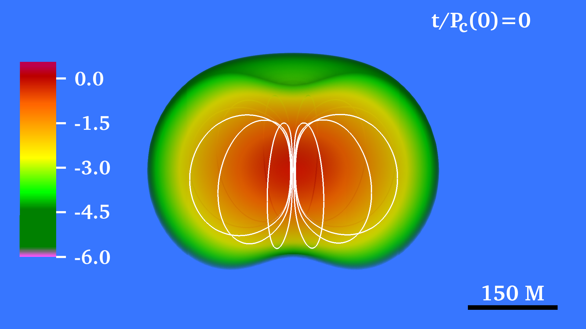
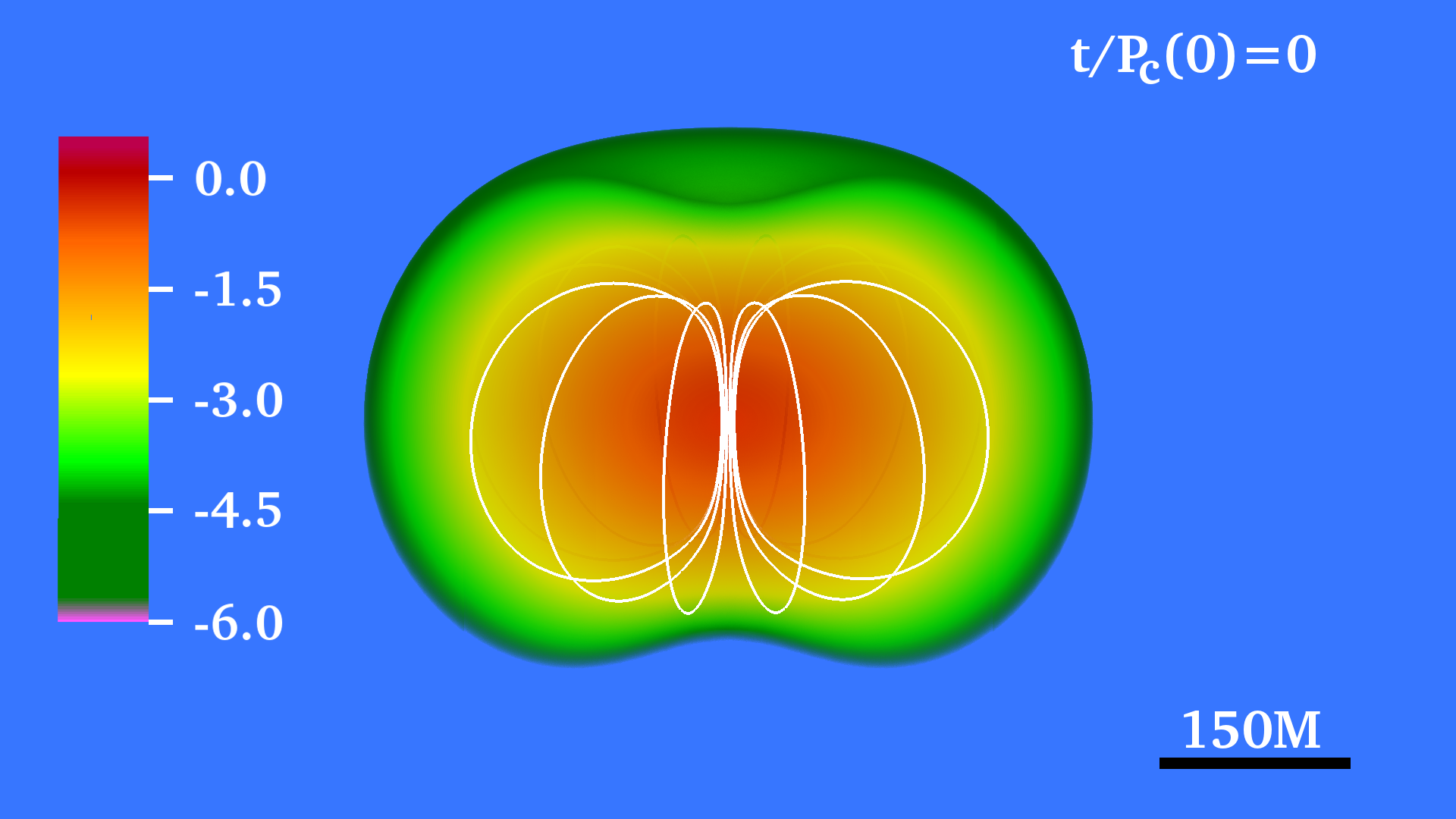
The star is seeded with a dipole-like, dynamically weak magnetic field confined to the stellar interior (see left panels in Fig. 1). The field is generated by the vector potential Sun et al. (2017, 2018),
| (18) |
where , , and are constants that determine the strength, the degree of central condensation, and the confinement of the magnetic fields, respectively. Following Sun et al. (2017, 2018), is set to times the initial maximum value of the pressure and to . We then set the amplitude such that for the two cases. The choice of the field strength is based on a compromise between insuring computationally achievable Alfvén and viscous damping timescales and preventing significant departures from hydrostatic equilibrium triggered by a dynamically strong magnetic field.
We cover the computational grid with a tenuous atmosphere with constant density following the standard setup in hydrodynamic and MHD simulations, where is the maximum rest-mass density at . The key initial parameters are summarized in Tables 1, and 2.
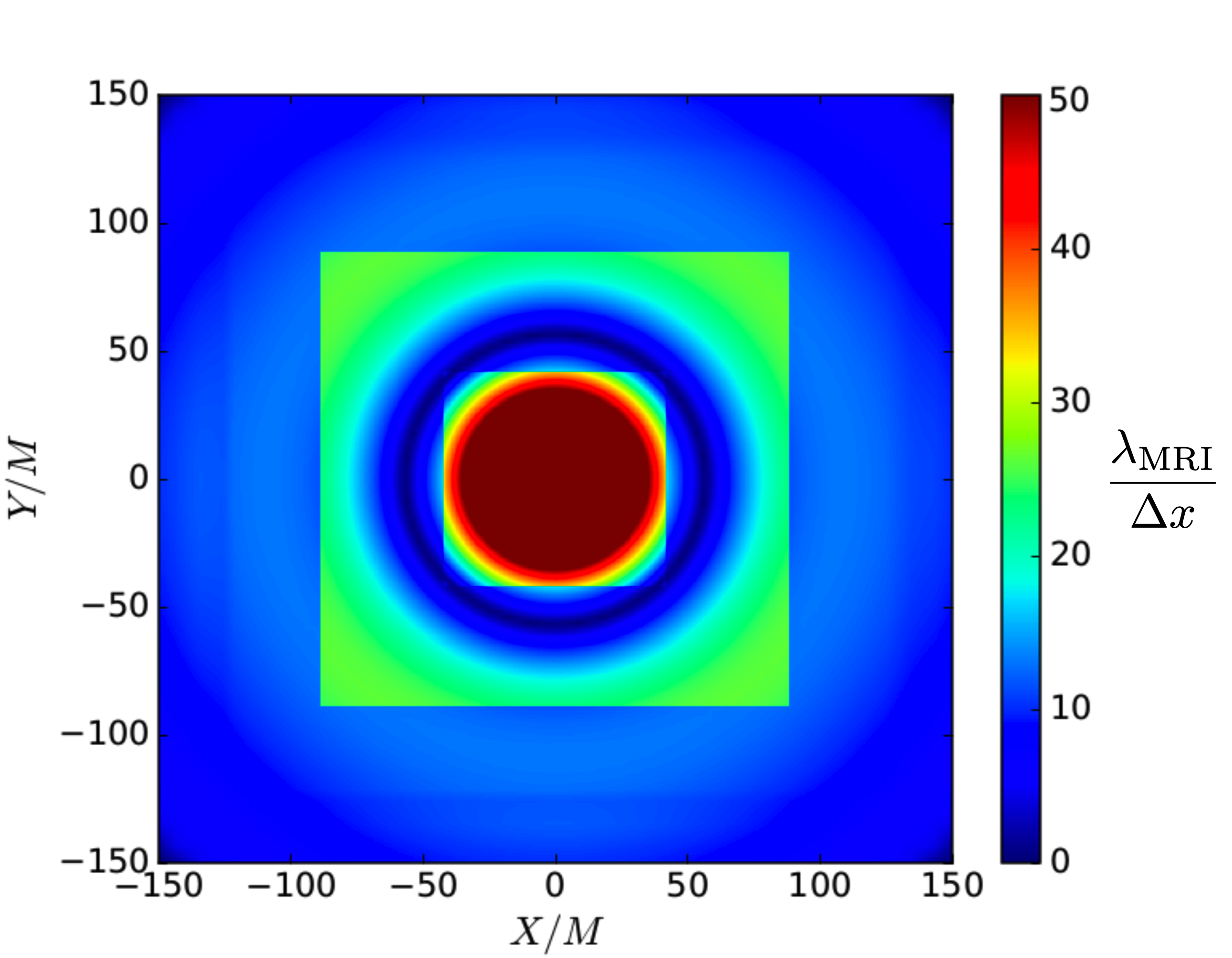
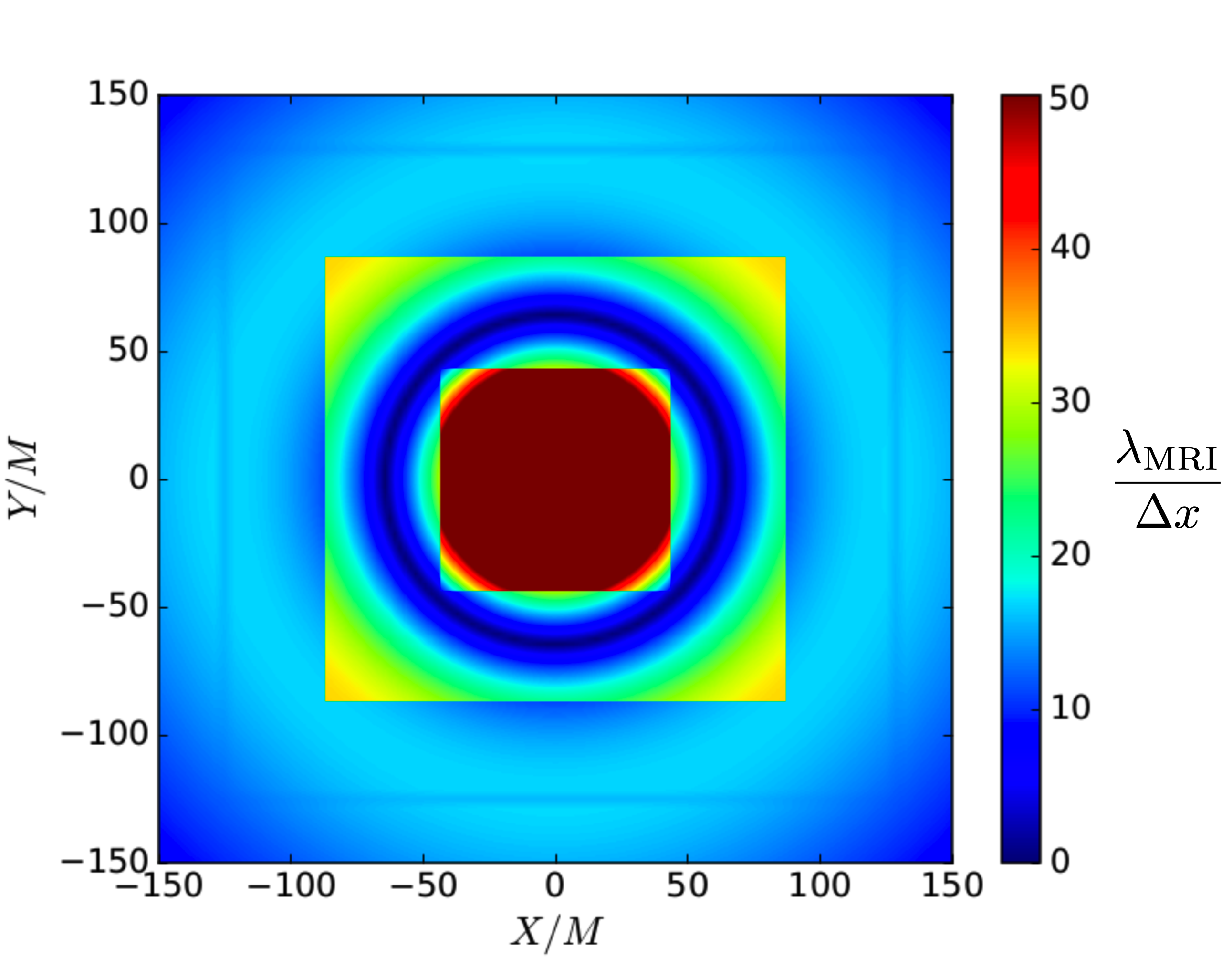
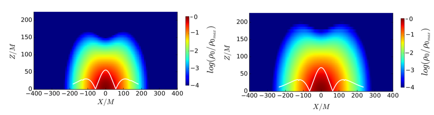
Before we start the numerical evolution of the above stars, we verify that MRI will be properly captured in our system. Following Gold et al. (2014), we check that: a) the magnetic field generated by the vector potential in Eq. 18 satisfies , a condition need to trigger the instability. b) The wavelength of the fastest-growing mode should be resolved by more than grid points Shibata et al. (2006); Sano et al. (2004); Shiokawa et al. (2012). We plot the quality factor on the equatorial plane, with the local grid spacing. As is showed in Fig. 2, we resolved by more than grid points in the bulk of our stellar models except for the ring-shaped region where the magnetic field flips direction. c) The wavelength should fit in the star. Fig. 3 shows along with the rest-mass density on the meridional plane. It is clear that the wavelength of the fastest-growing mode fits in the star. We conclude therefore that the MRI will be resolved and operating during the evolution of our stellar models.
IV Methods and Diagnostics
We solve Einstein’s equations for the gravitational field coupled to the equations of MHD for the matter and magnetic field. Numerically, we use the moving–grid adaptive mesh refinement (AMR) Illinois GRMHD code embedded in the Cactus222http://www.cactuscode.org/Carpet333http://www.carpetcode.org infrastructure. The code solves the Baumgarte–Shapiro–Shibata–Nakamura (BSSN) formulation of the Einstein’s equations Shibata and Nakamura (1995); Baumgarte and Shapiro (1998) to evolve the metric and employs moving puncture gauge conditions Baker et al. (2006); Campanelli et al. (2006). Here, we solve the equation for the shift vector in first-order form (see e.g. Hinder et al. (2014); Ruiz et al. (2011)) with the shift parameter for N29 case and for N295 case, with the ADM mass of the system. In solving the MHD equations, the code introduces a vector potential (see Eqs. (8)-(9) in Etienne et al. (2012)) in order to maintain the divergence–free condition of the magnetic field. The code solves the MHD equations in a conservative formulation (see Eqs.(27)-(29) in Etienne et al. (2010)) using high-resolution shock-capturing methods Duez et al. (2005). In addition, a generalized Lorenz gauge Etienne et al. (2012); Farris et al. (2012) is used to avoid the spurious magnetic fields between AMR levels due to numerical interpolations. As the standard numerical tool, the Illinois GRMHD code has been extensively tested and has performed multiple simulations, including merging magnetized compact objects and the collapsing massive stars (see e.g. Etienne et al. (2012); Paschalidis et al. (2013); Sun et al. (2017); Khan et al. (2018); Sun et al. (2018) and references therein for the suite of tests).
| Case | Grid hierarchy | |||
|---|---|---|---|---|
| N29 | ||||
| N295 |
To verify the reliability of our simulations, we monitor the normalized Hamiltonian and momentum constraints employing Eqs.(40)-(43) in Etienne et al. (2008), which remain below during the evolution. We verify the conservation of the total mass and total angular momentum computed using Eqs.(9)-(10) in Etienne et al. (2009), which coincides with the ADM mass and the ADM angular momentum at infinity, as well as the conservation of the rest-mass described by Eq.(11) in Etienne et al. (2009). We find that in the two cases listed in Table 1 , , and deviate from their initial values by only along the whole evolution. We also monitor the conservation of the binding energy , which may be decomposed according to
| (19) | |||||
where is the internal (thermal) energy, is the rotational kinetic energy, is the magnetic energy, and is gravitational potential energy. These quantities are calculated as follows:
| (20) |
| (21) |
| (22) |
and
| (23) |
where is the proper volume element with the lapse function, and the conformal exponent , where is the determinant of the three-metric , and is the specific internal energy. For the evolution, we use a -law EOS, and allow for shock heating. Here denotes the rest-mass density. We set the adiabatic index to for N29 and to for N295.
To properly resolve the magnetic instabilities, in the two equilibrium stellar models in Table 1, we use one set of mesh nested refinement boxes centered at the star. The finest box has a grid spacing of , and the star is resolved by more than 250 grid points across the diameter. The grid hierarchy for each case is summarized in Table 3. We impose reflection symmetry across the equatorial plane ().
V Numerical Results
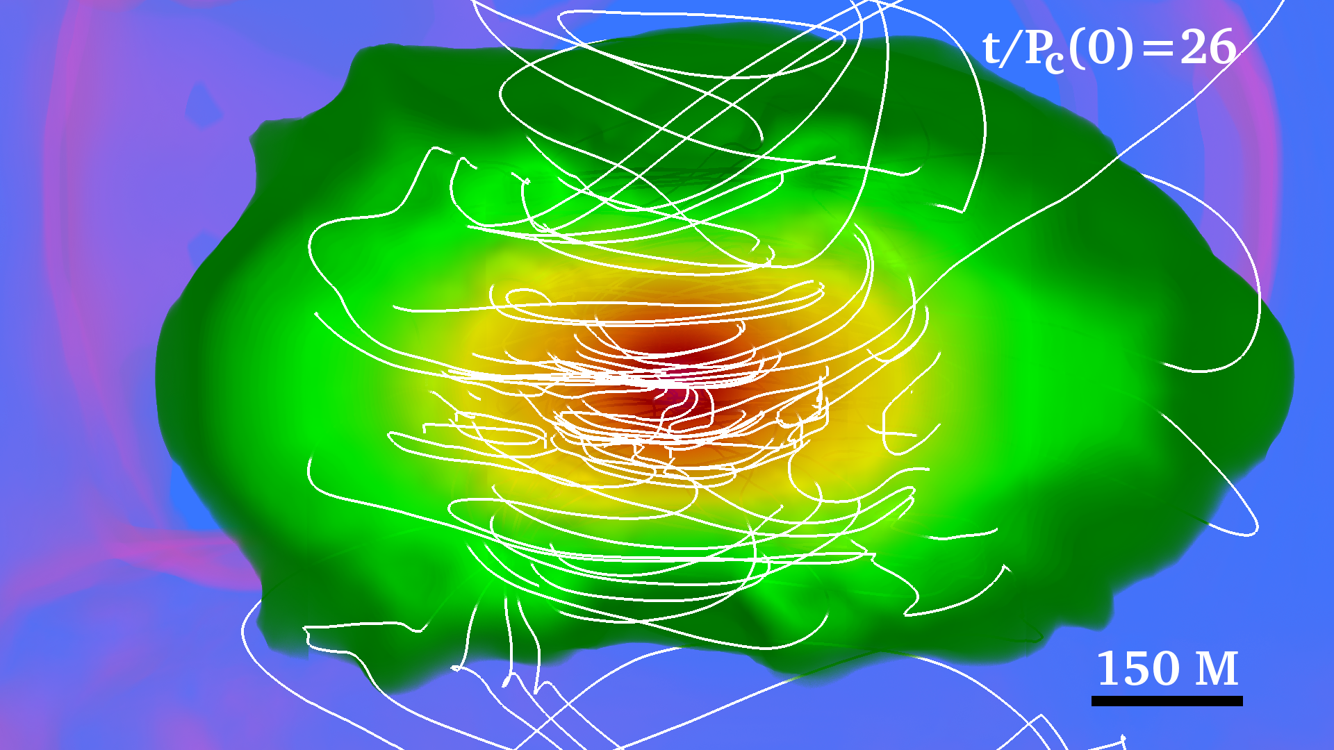
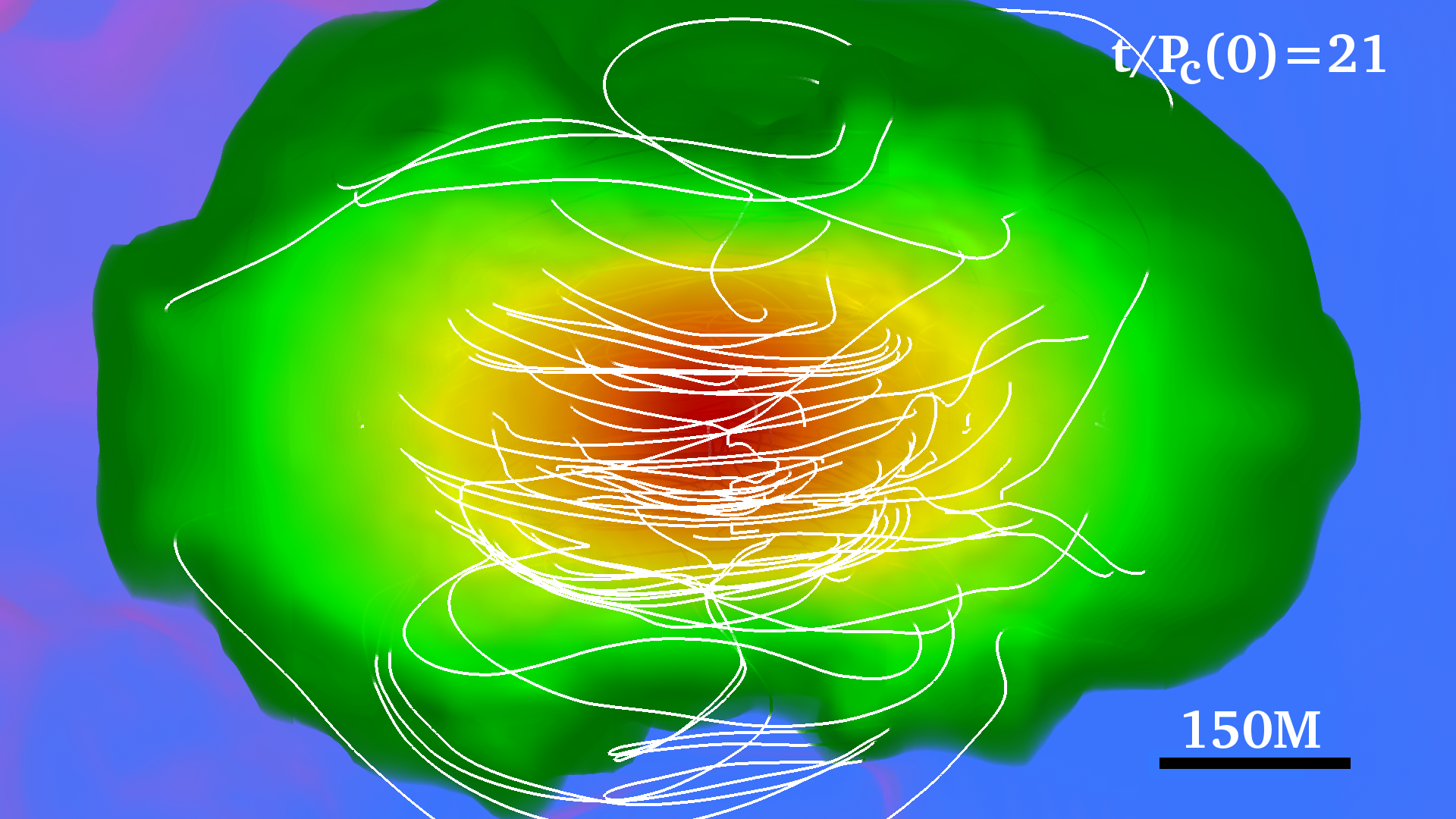
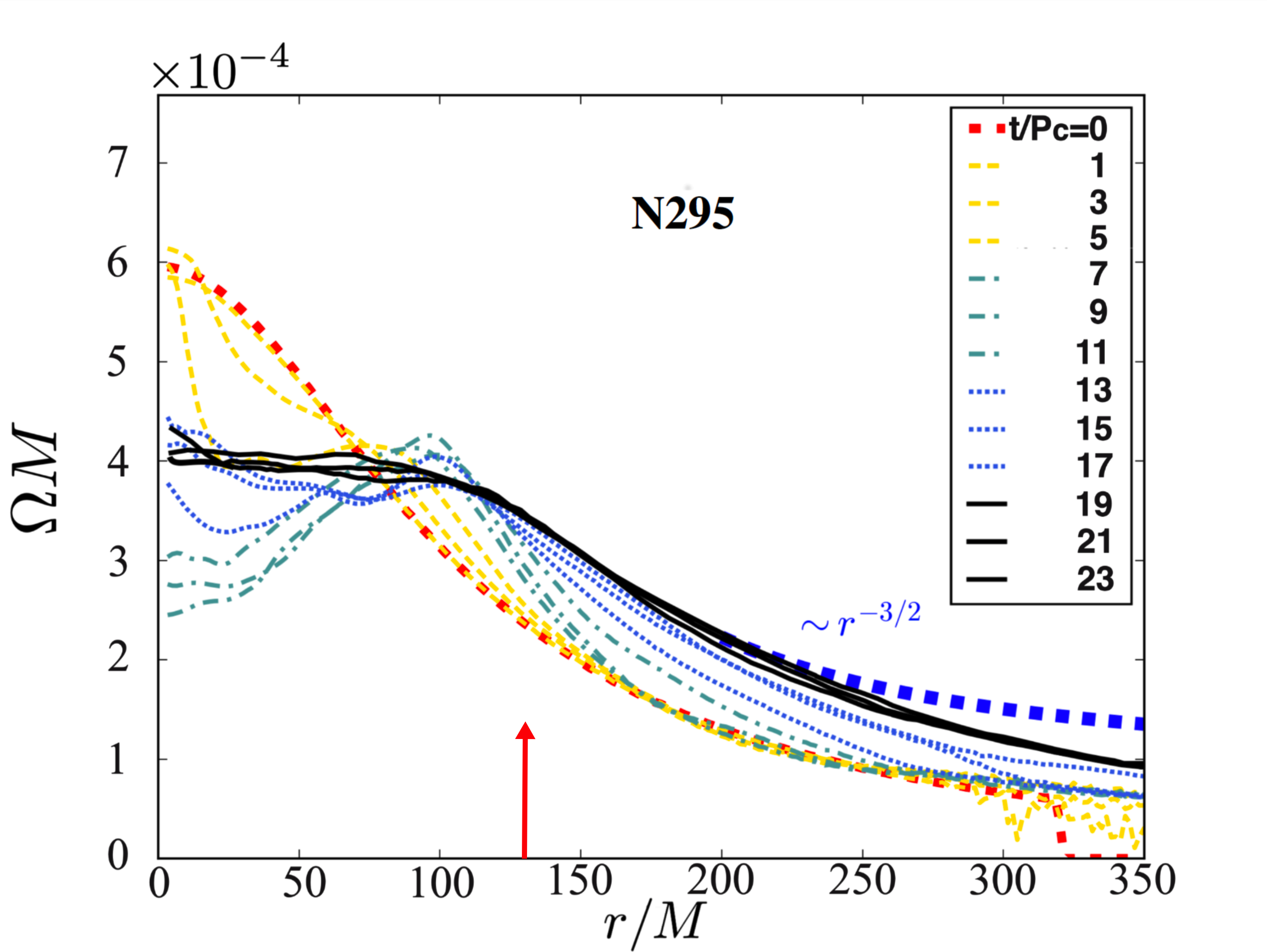
The basic dynamics and final outcome of our two cases listed in Table 1 are similar. Redistribution of angular momentum via magnetic winding and a turbulent viscosity triggered by magnetic instabilities in the bulk of the star induces the formation of a massive and near uniformly rotating inner core wrapped by a low-density Keplerian-like disk (see right panels in Fig. 1).
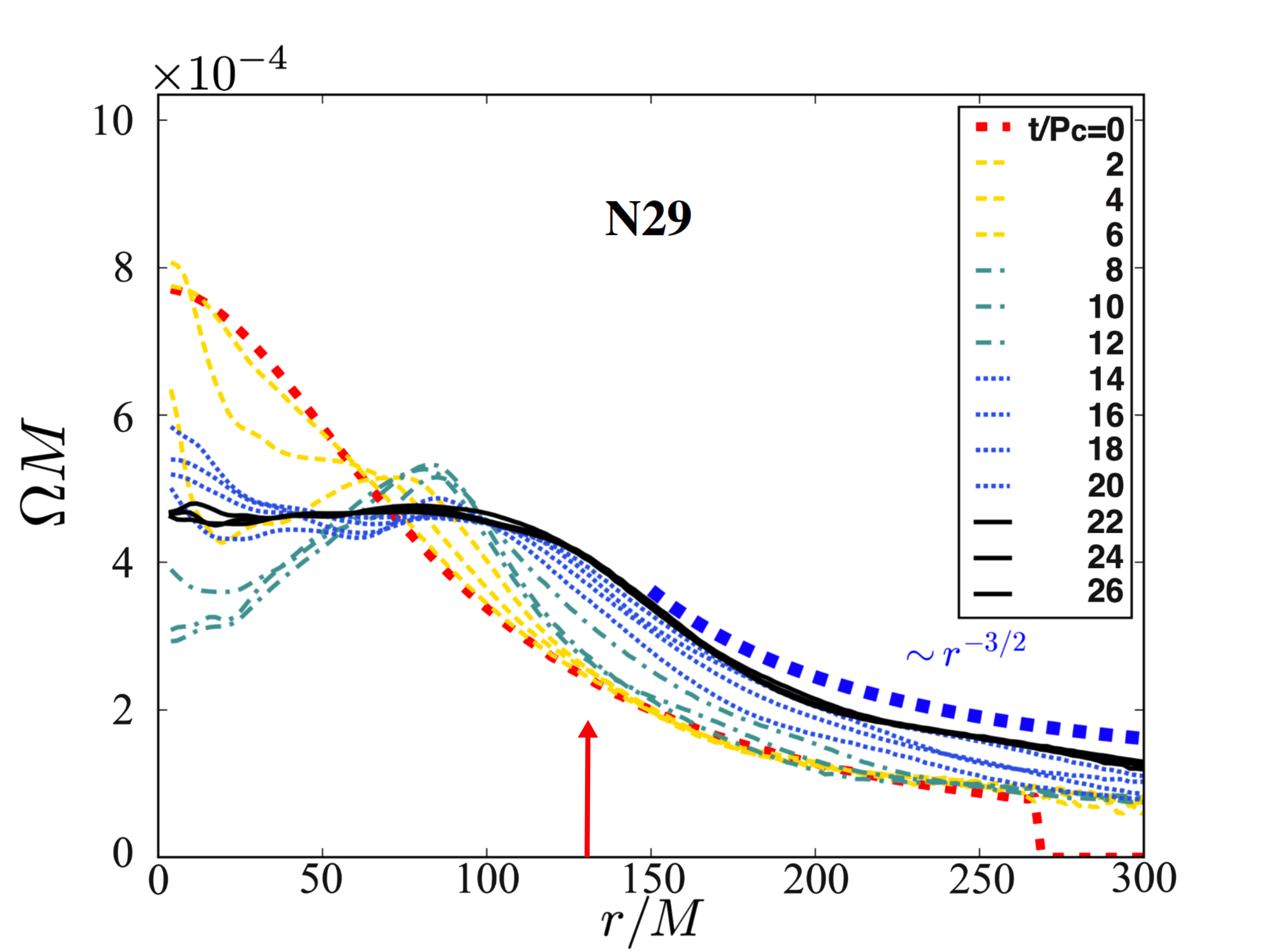
During the early phase of the stellar evolution, the dynamically weak magnetic field has a negligible back-reaction on the fluid. The poloidal frozen-in magnetic field is advected with the fluid and wound into a predominantly toroidal configuration. Differential rotation in the bulk of the star stretches the field lines, which in turn amplifies the toroidal component of the magnetic field (magnetic winding) and increases the magnetic stresses. After about two rotation periods (see Fig. 4), back-reaction of the magnetic field is large enough to change the fluid motion and to redistribute the angular momentum from the inner layers of the star to the outer regions Shibata (2015). This effect continues as long as the condition is maintained.
On the other hand, the timescale for the MRI can be estimated as
| (24) |
where is the average initial angular velocity. So, in the early phase of the stellar evolution, the MRI is quickly triggered. This instability induces an effective viscosity that eventually induces an exponential growth of the magnetic energy (see Fig. 5). Once the magnetic turbulence is fully developed, the angular momentum is redistributed by the turbulent viscosity from the inner (rapidly rotating) region to the outer (slowly rotating) region. This effect continues as long as the condition is satisfied. Notice that at inner layers of the star have an angular velocity that has a positive radial gradient (see Fig. 4). So, at this time magnetic winding is mainly the mechanism that redistributes the angular momentum from the inner to the outer regions of the star.
Therefore, both magnetic winding and the MRI enhance the angular momentum redistribution. It causes the contraction of the inner stellar layers and the increase of central density, forming a massive core. We define the core as the stellar region with rest-mass density where is the initial maximum rest-mass density. We estimate that, near to the end of the simulation, the radius of the inner core in the two stellar models considered here is roughly (see right panels in Fig. 1). After about twenty rotation periods, magnetic viscosity, which is at least partially developed, and magnetic stresses triggered by the MRI (see Eq 8) and magnetic winding redistribute the angular momentum and bring the star to a new quasiequilibrium configuration: a nearly uniformly rotating central core + a Keplerian disk (see 4). The new configuration then evolves on a secular timescale and remains in a quasi-stationary equilibrium until the termination of the simulation.
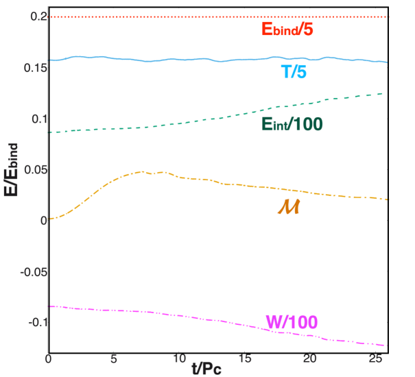
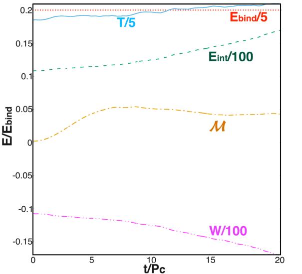
Time evolution of energies
As previously stated, during the early phase of the stellar evolution, both magnetic winding and the MRI enhance the magnetic energy . As shown in Fig. 5, the magnitude of increases by roughly three orders of magnitude by where is the initial central rotation period, and then decreases due to damped oscillations. The decrease of the magnetic energy is caused by turbulent viscosity triggered by the MRI and this serves to heat the gas. After about , the magnetic energy reaches a value of of the binding energy in case N29 and in case N295. The internal energy increases gradually with time, indicating continuous heating. The major heating energy coincides with the decrease of gravitational potential energy due to the contraction of the stellar core (see Eq. 11). Note that, is not the main heating source because throughout the evolution.
The rotational kinetic energy , on the other hand, remains nearly constant throughout the whole simulation in N29, where we observe very small fractional changes. As shown in Fig. 4, after , the inner core remnant spins at of the initial angular velocity of the star. In contrast, in N295 increases by around of its initial value. After , the inner core remnant spins at of the initial angular velocity of the star. Notice that the gravitational potential energy decreases faster in N295 than N29. This behavior suggests that the increase of comes from , indicating that the stiffer the EOS, the more difficult it is to transfer potential energy. These results display great differences from previous studies of magnetic braking of differential rotation in infinite cylinders and incompressible stars, where a substantial fraction of is transferred to Shapiro (2000); Cook et al. (2003); Liu and Shapiro (2004). However, the energy evolution of our models shares several similarities with the B1 model in the study of magnetic braking and damping of neutron stars Duez et al. (2006b), where a non-hypermassive and “ultra-spinning” (angular momentum exceeding the maximum for uniform rotation at the same rest mass) polytrope with an effective turbulent viscosity were evolved.
VI Conclusions
The growth of seed density perturbations and their fragmentation in massive stars with a high degree of differential rotation undergoing collapse has been suggested as a viable channel for binary black hole formation. Here we illustrate the likely fate of such massive stars during their prior, stable, evolutionary lifetime. We build GR stellar models described by a polytropic EOS with polytropic index and , with the same differential rotation law as in Zink et al. (2006, 2007). We endowed the stars with a dynamically weak, poloidal magnetic field confined to the stellar interior. The ratio of initial magnetic energy to gravitational potential energy is .
We found that during the early phase of the evolution, magnetic winding and the MRI greatly amplify the initial magnetic field. During that period, the magnetic field is increased by times its initial value. At the same time, angular momentum from the inner layers of the star is transported outward. The inner layers then shrink and form a massive inner core in which the differential rotation eventually (around twenty rotation periods) is fully damped. Therefore, prior to reaching the state of gravitational radial instability, magnetic braking and turbulent magnetic viscosity drive a massive star to a new quasi-equilibrium state. This state consists of a uniformly rotating central core surrounded by a low-density Keplerian disk. These are not the matter or rotation profiles that will lead to growth and fragmentation of density perturbations during catastrophic collapse.
We estimated various physical timescales that determine the stellar evolution of the stellar models considered here. Using the initial parameters of our GR stellar models, we found that the timescales obey a natural hierarchy (see Eq. 13). This hierarchy shows that during the normal evolutionary lifetime of a star, a sufficiently high degree of differential rotation required to trigger perturbation growth and fragmentation leading to binary BH formation during collapse will be suppressed. Our numerical results should describe the fate of stars with characteristic masses greater than several hundred solar masses, which are possible progenitors of binary massive stellar-mass BHs and IMBHs that produce GW signals detectable by LVSC.
Given our numerical results, we conclude that the binary black hole formation channel described in Reisswig et al. (2013) is not likely, assuming that the differentially rotating massive star that might undergo fragmentation during collapse experienced a long evolution phase in hydrostatic equilibrium before arriving at radial instability to collapse. During such a phase, even a small initial magnetic field will amplify and ultimately damp the differential rotation required to grow the seed perturbations that trigger fission or fragmentation. However, if a high degree of differential rotation is resuscitated following some sudden catastrophic event, such as a massive star binary collision and merger, followed by a sudden collapse, then it may still be possible for the fragmentation-binary BH formation mechanism to be triggered. The likelihood of such an event remains to be determined.
We remark that the values of the parameter found numerically depend strongly on the adopted resolution. As it has been shown in Kiuchi et al. (2018); Hawley et al. (2013, 2011) the higher the resolution, the higher the alpha parameter. Therefore, it is expected that in higher order numerical simulations the viscosity timescale, the time over which the turbulent viscosity damps differential rotation, will be shortened. But, magnetic winding and the MRI still will drive a massive star to a new quasi-equilibrium state that consists of a uniformly rotating central core surrounded by a low-density Keplerian disk. Our basic conclusion during its lifetime therefore will remain unaffected, though the hierarchy of timescales in Eq. 13 may change.
Acknowledgements.
We thank V. Paschalidis for useful discussions and the Illinois Relativity group REU team (K. Nelli) for assistance in creating Fig. 1. This work has been supported in part by National Science Foundation (NSF) Grant PHY-1602536 and PHY-1662211, and NASA Grant 80NSSC17K0070 at the University of Illinois at Urbana-Champaign. This work made use of the Extreme Science and Engineering Discovery Environment (XSEDE), which is supported by National Science Foundation grant number TG-MCA99S008. This research is part of the Blue Waters sustained-petascale computing project, which is supported by the National Science Foundation (awards OCI-0725070 and ACI-1238993) and the State of Illinois. Blue Waters is a joint effort of the University of Illinois at Urbana-Champaign and its National Center for Supercomputing Applications.References
- Abbott et al. (2016a) B. P. Abbott et al. (LIGO Scientific Collaboration and Virgo Collaboration), Phys. Rev. Lett. 116, 061102 (2016a), URL http://link.aps.org/doi/10.1103/PhysRevLett.116.061102.
- Abbott et al. (2016b) B. Abbott et al. (Virgo, LIGO Scientific), Phys. Rev. Lett. 116, 241103 (2016b).
- Abbott et al. (2017a) B. P. Abbott et al. (LIGO Scientific and Virgo Collaboration), Phys. Rev. Lett. 118, 221101 (2017a), URL https://link.aps.org/doi/10.1103/PhysRevLett.118.221101.
- Abbott et al. (2017b) B. P. Abbott et al. (Virgo, LIGO Scientific), Phys. Rev. Lett. 119, 141101 (2017b), eprint 1709.09660.
- Abbott et al. (2017) B. P. Abbott, R. Abbott, T. D. Abbott, F. Acernese, K. Ackley, C. Adams, T. Adams, P. Addesso, R. X. Adhikari, V. B. Adya, et al., The Astrophysical Journal Letters 851, L35 (2017), eprint 1711.05578.
- Abbott et al. (2018) B. P. Abbott et al. (Virgo, LIGO Scientific) (2018), eprint arXiv:1811.12907.
- Remillard and McClintock (2006) R. A. Remillard and J. E. McClintock, Annual Review of Astronomy and Astrophysics 44, 49 (2006), eprint https://doi.org/10.1146/annurev.astro.44.051905.092532, URL https://doi.org/10.1146/annurev.astro.44.051905.092532.
- Bird et al. (2016) S. Bird, I. Cholis, J. B. Muñoz, Y. Ali-Haïmoud, M. Kamionkowski, E. D. Kovetz, A. Raccanelli, and A. G. Riess, Phys. Rev. Lett. 116, 201301 (2016), URL https://link.aps.org/doi/10.1103/PhysRevLett.116.201301.
- Carr et al. (2016) B. Carr, F. Kühnel, and M. Sandstad, Phys. Rev. D 94, 083504 (2016), URL https://link.aps.org/doi/10.1103/PhysRevD.94.083504.
- Clesse and Garcí a-Bellido (2017) S. Clesse and J. Garcí a-Bellido, Physics of the Dark Universe 15, 142 (2017), ISSN 2212-6864, URL http://www.sciencedirect.com/science/article/pii/S2212686416300553.
- Eroshenko (2018) Y. N. Eroshenko, Journal of Physics: Conference Series 1051, 012010 (2018), URL http://stacks.iop.org/1742-6596/1051/i=1/a=012010.
- Schrøder et al. (2018) S. L. Schrøder, A. Batta, and E. Ramirez-Ruiz, The Astrophysical Journal Letters 862, L3 (2018), URL http://stacks.iop.org/2041-8205/862/i=1/a=L3.
- Tutukov and YungelSon (1993) A. V. Tutukov and L. R. YungelSon, Monthly Notices of the Royal Astronomical Society 260, 675 (1993), URL http://dx.doi.org/10.1093/mnras/260.3.675.
- Voss and Tauris (2003) R. Voss and T. M. Tauris, Monthly Notices of the Royal Astronomical Society 342, 1169 (2003), URL http://dx.doi.org/10.1046/j.1365-8711.2003.06616.x.
- Woosley et al. (2002) S. E. Woosley, A. Heger, and T. A. Weaver, Rev. Mod. Phys. 74, 1015 (2002).
- Belczynski et al. (2010) K. Belczynski, T. Bulik, C. L. Fryer, A. Ruiter, F. Valsecchi, J. S.Vink, and J. R. Hurley, The Astrophysical Journal 714, 1217 (2010), URL http://stacks.iop.org/0004-637X/714/i=2/a=1217.
- Dominik et al. (2013) M. Dominik, K. Belczynski, C. Fryer, D. E. Holz, E. Berti, T. Bulik, I. Mandel, and R. O’Shaughnessy, Astrophys. J. 779, 72 (2013), eprint 1308.1546.
- Kinugawa et al. (2014) T. Kinugawa, K. Inayoshi, K. Hotokezaka, D. Nakauchi, and T. Nakamura, Monthly Notices of the Royal Astronomical Society 442, 2963 (2014), URL http://dx.doi.org/10.1093/mnras/stu1022.
- Belczynski et al. (2016) K. Belczynski, D. E. Holz, T. Bulik, and R. O’Shaughnessy, Nature (London) 534, 512 (2016), eprint 1602.04531.
- Stevenson et al. (2013) S. Stevenson, A. Vigna-G mez, I. Mandel, J. W. Barrett, C. J. Neijssel, D. Perkins, and S. E. de Mink, Nat. Comm. 8, 14906 (2013), eprint 1205.6871, URL http://dx.doi.org/10.1038/ncomms14906.
- Kalogera et al. (2004) V. Kalogera, C. Kim, D. R. Lorimer, M. Burgay, N. D’Amico, A. Possenti, R. N. Manchester, A. G. Lyne, B. C. Joshi, M. A. McLaughlin, et al., The Astrophysical Journal Letters 601, L179 (2004), URL http://stacks.iop.org/1538-4357/601/i=2/a=L179.
- Marchant et al. (2016) P. Marchant, N. Langer, P. Podsiadlowski, T. M. Tauris, and T. J. Moriya, Astron. Astrophys. 588, A50 (2016), URL https://ui.adsabs.harvard.edu/#abs/2016A&A...588A..50M.
- de Mink and Mandel (2016) S. E. de Mink and I. Mandel, Monthly Notices of the Royal Astronomical Society 460, 3545 (2016), URL http://dx.doi.org/10.1093/mnras/stw1219.
- Zackay et al. (2019) B. Zackay, T. Venumadhav, L. Dai, J. Roulet, and M. Zaldarriaga (2019), eprint arXiv:1902.10331.
- Note (1) Note1, however, low-metallicity AGN is extremely rare from observations. For details, see, e.g., http://dx.doi.org/10.1111/j.1365-2966.2006.10812.x.
- Rodriguez et al. (2016a) C. L. Rodriguez, M. Morscher, L. Wang, S. Chatterjee, F. A. Rasio, and R. Spurzem, Mon. Not. Roy. Astron. Soc. 463, 2109 (2016a), URL http://dx.doi.org/10.1093/mnras/stw2121.
- Chatterjee et al. (2017) S. Chatterjee, C. L. Rodriguez, and F. A. Rasio, The Astrophysical Journal 834, 68 (2017), URL http://stacks.iop.org/0004-637X/834/i=1/a=68.
- Fishbach et al. (2017) M. Fishbach, D. E. Holz, and B. Farr, The Astrophysical Journal Letters 840, L24 (2017), URL http://stacks.iop.org/2041-8205/840/i=2/a=L24.
- Rodriguez et al. (2016b) C. L. Rodriguez, C.-J. Haster, S. Chatterjee, V. Kalogera, and F. A. Rasio, Astrophys. J. Lett. 824, L8 (2016b), URL http://stacks.iop.org/2041-8205/824/i=1/a=L8.
- Miller and Colbert (2004) M. C. Miller and E. J. M. Colbert, Int. J. Mod. Phys. D13, 1 (2004), eprint astro-ph/0308402.
- Abbott et al. (2017) B. P. Abbott et al. (LIGO Scientific Collaboration and Virgo Collaboration), Phys. Rev. D 96, 022001 (2017), URL https://link.aps.org/doi/10.1103/PhysRevD.96.022001.
- Gair et al. (2011) J. R. Gair, I. Mandel, M. C. Miller, and M. Volonteri, Gen. Relativ. Gravit. 43, 485 (2011), eprint gr-qc/0907.5450, URL https://doi.org/10.1007/s10714-010-1104-3.
- Connaughton et al. (2016) V. Connaughton et al., The Astrophysical Journal Letters 826, L6 (2016), URL http://stacks.iop.org/2041-8205/826/i=1/a=L6.
- Verrecchia et al. (2017) F. Verrecchia, M. Tavani, A. Ursi, A. Argan, C. Pittori, I. Donnarumma, A. Bulgarelli, F. Fuschino, C. Labanti, and et al., The Astrophysical Journal Letters 847, L20 (2017), URL http://stacks.iop.org/2041-8205/847/i=2/a=L20.
- Lyutikov (2016) Lyutikov (2016), eprint astro-ph.HE/1602.07352.
- Khan et al. (2018) A. Khan, V. Paschalidis, M. Ruiz, and S. L. Shapiro, Phys. Rev. D97, 044036 (2018), eprint 1801.02624.
- Loeb (2016) A. Loeb, The Astrophysical Journal Letters 819, L21 (2016), URL http://stacks.iop.org/2041-8205/819/i=2/a=L21.
- Fedrow et al. (2017) J. M. Fedrow, C. D. Ott, U. Sperhake, J. Blackman, R. Haas, C. Reisswig, and A. De Felice, Phys. Rev. Lett. 119, 171103 (2017), URL https://link.aps.org/doi/10.1103/PhysRevLett.119.171103.
- Dai et al. (2017) L. Dai, J. C. McKinney, and M. C. Miller, Monthly Notices of the Royal Astronomical Society: Letters 470, L92 (2017), URL http://dx.doi.org/10.1093/mnrasl/slx086.
- D’Orazio and Loeb (2018) D. J. D’Orazio and A. Loeb, Phys. Rev. D97, 083008 (2018), eprint 1706.04211.
- Gold et al. (2014) R. Gold, V. Paschalidis, Z. B. Etienne, S. L. Shapiro, and H. P. Pfeiffer, Phys.Rev. D89, 064060 (2014), eprint 1312.0600.
- Gold et al. (2014) R. Gold, V. Paschalidis, M. Ruiz, S. L. Shapiro, Z. B. Etienne, and H. P. Pfeiffer, Phys. Rev. D 90, 104030 (2014), eprint 1410.1543.
- Baumgarte and Shapiro (1999) T. W. Baumgarte and S. L. Shapiro, Astrophys. J. 526, 941 (1999).
- Shibata and Shapiro (2002) M. Shibata and S. L. Shapiro, Astrophys. J. Lett. 572, L39 (2002), eprint astro-ph/0205091.
- Saijo et al. (2002) M. Saijo, T. W. Baumgarte, S. L. Shapiro, and M. Shibata, The Astrophysical Journal 569, 349 (2002).
- Zink et al. (2006) B. Zink, N. Stergioulas, I. Hawke, C. D. Ott, E. Schnetter, and E. Müller, Phys. Rev. Lett. 96, 161101 (2006), eprint gr-qc/0501080.
- Saijo and Hawke (2009) M. Saijo and I. Hawke, Phys. Rev. D 80, 064001 (2009).
- Shibata et al. (2016) M. Shibata, H. Uchida, and Y. Sekiguchi, Astrophys. J. 818, 157 (2016), astro-ph.HE/1604.00643.
- Butler et al. (2018) S. P. Butler, A. R. Lima, T. W. Baumgarte, and S. L. Shapiro, Mon. Not. Roy. Astron. Soc. 477, 3694 (2018).
- Sun et al. (2017) L. Sun, V. Paschalidis, M. Ruiz, and S. Shapiro, Phys. Rev. D 96, 043006 (2017), eprint astro-ph.HE:1704.04502.
- Sun et al. (2018) L. Sun, M. Ruiz, and S. Shapiro, Phys. Rev. D 98, 103008 (2018), eprint 1807.07970.
- Bodenheimer and Ostriker (1973) P. Bodenheimer and J. P. Ostriker, Astrophys. J. 180, 159 (1973).
- New and Shapiro (2001a) K. C. B. New and S. L. Shapiro, Class. Quantum Grav. 18, 3965 (2001a), eprint astro-ph/0009095.
- New and Shapiro (2001b) K. C. B. New and S. L. Shapiro, Astrophys. J. 548, 439 (2001b), eprint astro-ph/0010172.
- Zink et al. (2007) B. Zink, N. Stergioulas, I. Hawke, C. D. Ott, E. Schnetter, and E. Müller, Phys. Rev. D 76, 024019 (2007), URL https://link.aps.org/doi/10.1103/PhysRevD.76.024019.
- Reisswig et al. (2013) C. Reisswig, C. Ott, E. Abdikamalov, R. Haas, P. Moesta, and E. Schnetter, Phys. Rev. Lett. 111, 151101 (2013), eprint 1304.7787.
- Shapiro (2000) S. L. Shapiro, Astrophys. J. 544, 397 (2000).
- Cook et al. (2003) J. N. Cook, S. L. Shapiro, and B. C. Stephens, Astrophys. J. 599, 1272 (2003).
- Liu and Shapiro (2004) Y. T. Liu and S. L. Shapiro, Phys. Rev. D 69, 044009 (2004), URL https://link.aps.org/doi/10.1103/PhysRevD.69.044009.
- Etienne et al. (2006) Z. B. Etienne, Y. T. Liu, and S. L. Shapiro, Phys. Rev. D74, 044030 (2006), eprint astro-ph/0609634.
- Duez et al. (2004) M. D. Duez, Y. T. Liu, S. L. Shapiro, and B. C. Stephens, Phys. Rev. D 69, 104030 (2004), eprint gr-qc/0402502.
- Duez et al. (2006a) M. D. Duez, Y. T. Liu, S. L. Shapiro, M. Shibata, and B. C. Stephens, Phys. Rev. Lett. 96, 031101 (2006a), eprint astro-ph/0510653.
- Duez et al. (2006b) M. D. Duez, Y. T. Liu, S. L. Shapiro, M. Shibata, and B. C. Stephens, Phys. Rev. D 73, 104015 (2006b), gr-qc/0605331.
- Shibata et al. (2006) M. Shibata, Y. T. Liu, S. L. Shapiro, and B. C. Stephens, Phys. Rev. D 74, 104026 (2006), URL https://doi.org/10.1103/PhysRevD.74.104026.
- Penna et al. (2010) R. F. Penna, J. C. McKinney, R. Narayan, A. Tchekhovskoy, R. Shafee, and J. E. McClintock, Monthly Notices of the Royal Astronomical Society 408, 752 (2010), URL http://dx.doi.org/10.1111/j.1365-2966.2010.17170.x.
- Baumgarte and Shapiro (2010) T. W. Baumgarte and S. L. Shapiro, Numerical Relativity: Solving Einstein’s Equations on the Computer (Cambridge University Press, 2010).
- Cook et al. (1992) G. B. Cook, S. L. Shapiro, and S. A. Teukolsky, Astrophys. J. 398, 203 (1992).
- Cook et al. (1994) G. B. Cook, S. L. Shapiro, and S. A. Teukolsky, Astrophys. J. 422, 227 (1994).
- Cook et al. (1994) G. B. Cook, S. L. Shapiro, and S. A. Teukolsky, Astrophys. J. 424, 823 (1994).
- Sano et al. (2004) T. Sano, S.-i. Inutsuka, N. J. Turner, and J. M. Stone, Astrophys. J. 605, 321 (2004), eprint astro-ph/0312480.
- Shiokawa et al. (2012) H. Shiokawa, J. C. Dolence, C. F. Gammie, and S. C. Noble, The Astrophysical Journal 744, 187 (2012), URL http://stacks.iop.org/0004-637X/744/i=2/a=187.
- Note (2) Note2, http://www.cactuscode.org.
- Note (3) Note3, http://www.carpetcode.org.
- Shibata and Nakamura (1995) M. Shibata and T. Nakamura, Phys. Rev. D 52, 5428 (1995).
- Baumgarte and Shapiro (1998) T. W. Baumgarte and S. L. Shapiro, Phys. Rev. D 59, 024007 (1998), eprint gr-qc/9810065.
- Baker et al. (2006) J. G. Baker, J. Centrella, D.-I. Choi, M. Koppitz, and J. van Meter, Phys. Rev. Lett. 96, 111102 (2006), eprint gr-qc/0511103.
- Campanelli et al. (2006) M. Campanelli, C. O. Lousto, P. Marronetti, and Y. Zlochower, Phys. Rev. Lett. 96, 111101 (2006), eprint gr-qc/0511048.
- Hinder et al. (2014) I. Hinder, A. Buonanno, M. Boyle, Z. B. Etienne, J. Healy, et al., Classical Quantum Gravity 31, 025012 (2014), eprint 1307.5307.
- Ruiz et al. (2011) M. Ruiz, D. Hilditch, and S. Bernuzzi, Phys. Rev. D 83, 024025 (2011), eprint 1010.0523.
- Etienne et al. (2012) Z. B. Etienne, V. Paschalidis, Y. T. Liu, and S. L. Shapiro, Phys. Rev. D 85, 024013 (2012).
- Etienne et al. (2010) Z. B. Etienne, Y. T. Liu, and S. L. Shapiro, Phys.Rev. D82, 084031 (2010).
- Duez et al. (2005) M. D. Duez, Y. T. Liu, S. L. Shapiro, and B. C. Stephens, Phys. Rev. D 72, 024028 (2005), URL https://link.aps.org/doi/10.1103/PhysRevD.72.024028.
- Farris et al. (2012) B. D. Farris, R. Gold, V. Paschalidis, E. Z. B., and S. Shapiro, Phys. Rev. Lett. 109, 221102 (2012), eprint 1207.3354.
- Paschalidis et al. (2013) V. Paschalidis, Z. B. Etienne, and S. L. Shapiro, Phys.Rev. D88, 021504 (2013).
- Etienne et al. (2008) Z. B. Etienne, J. A. Faber, Y. T. Liu, S. L. Shapiro, K. Taniguchi, et al., Phys.Rev. D77, 084002 (2008).
- Etienne et al. (2009) Z. B. Etienne, Y. T. Liu, S. L. Shapiro, and T. W. Baumgarte, Phys. Rev. D79, 044024 (2009), eprint 0812.2245.
- Shibata (2015) M. Shibata, 100 Years of General Relativity (World Scientific Publishing Company, 2015), ISBN 9814699721.
- Kiuchi et al. (2018) K. Kiuchi, K. Kyutoku, Y. Sekiguchi, and M. Shibata, Phys. Rev. D97, 124039 (2018), eprint 1710.01311.
- Hawley et al. (2013) J. F. Hawley, S. A. Richers, X. Guan, and J. H. Krolik, Astrophys. J. 772, 102 (2013), eprint 1306.0243.
- Hawley et al. (2011) J. F. Hawley, X. Guan, and J. H. Krolik, Astrophys. J. 738, 84 (2011), eprint 1103.5987.