Magnetohydrodynamical torsional oscillations from thermo-resistive instability in hot jupiters
Abstract
Hot jupiter atmospheres may be subject to a thermo-resistive instability where an increase in the electrical conductivity due to ohmic heating results in runaway of the atmospheric temperature. We introduce a simplified one-dimensional model of the equatorial sub-stellar region of a hot jupiter which includes the temperature-dependence and time-dependence of the electrical conductivity, as well as the dynamical back-reaction of the magnetic field on the flow. This model extends our previous one-zone model to include the radial structure of the atmosphere. Spatial gradients of electrical conductivity strongly modify the radial profile of Alfvén oscillations, leading to steepening and downwards transport of magnetic field, enhancing dissipation at depth. We find unstable solutions that lead to self-sustained oscillations for equilibrium temperatures in the range – K, and magnetic field in the range – G. For a given set of parameters, self-sustained oscillations occur in a narrow range of equilibrium temperatures which allow the magnetic Reynolds number to alternate between large and small values during an oscillation cycle. Outside of this temperature window, the system reaches a steady state in which the effect of the magnetic field can be approximated as a magnetic drag term. Our results show that thermo-resistive instability is a possible source of variability in magnetized hot jupiters at colder temperatures, and emphasize the importance of including the temperature-dependence of electrical conductivity in models of atmospheric dynamics.
1 Introduction
Exoplanet surveys have detected nearly 500 hot jupiters (HJ), gas giants orbiting their host star with an orbit of , according to the data of exoplanet.eu (Schneider et al., 2011). Due to their proximity to their hosts, they are exposed to extreme irradiation and are assumed to be tidally locked. Such an arrangement results in interesting atmospheric dynamics, including a dayside to nightside flow driven by the gradient of temperature (Komacek & Showman, 2016), an equatorial superrotation driven by Rossby and Kelvin waves (Read & Lebonnois, 2018; Imamura et al., 2020) resulting in the zonal displacement of the hot spot away from the substellar point, and magnetic effects due to partial ionization in the atmosphere (Rogers & Komacek, 2014). Indeed, HJs may well be some of the most non-axisymmetric single astrophysical bodies known to date.
Even though the first discovery of a hot jupiter goes back a quarter of a century (Mayor & Queloz, 1995), some features of these planets are still not fully understood. Some of these unexplained observations are the larger than expected radii (Bodenheimer et al., 2001; Guillot & Showman, 2002; Baraffe et al., 2003; Bodenheimer et al., 2003; Laughlin et al., 2005; Thorngren et al., 2021), differences in dayside to nightside circulation efficiency (Cowan et al., 2007; Knutson et al., 2007; Crossfield et al., 2010; Cowan et al., 2012), and the westward winds observed in some hot jupiters (Armstrong et al., 2016; Dang et al., 2018; Jackson et al., 2019; Bell et al., 2019; von Essen et al., 2020) instead of the predicted eastward direction (Showman & Guillot, 2002; Cooper & Showman, 2005; Showman et al., 2009; Rauscher & Menou, 2010; Kataria et al., 2016), although many hot jupiters do show eastward flows (Knutson et al., 2007, 2009, 2012; Zellem et al., 2014).
A number of proposed explanations for these puzzles involve magnetism. The temperatures in HJs are sufficiently high for thermal ionization (Batygin & Stevenson, 2010; Perna et al., 2010a), in particular of alkali metals, which have low first ionization energies (Welbanks et al., 2019). It has been previously shown that ionization in the atmospheres of these gas giants results in coupling of winds with magnetic field generated deeper in the planet (Batygin & Stevenson, 2010; Perna et al., 2010a, b; Menou, 2012a). Magnetic interaction between the upper and lower envelopes of the HJs can slow down the atmospheric winds, and strong fields may even reverse the wind direction (Rogers & Komacek, 2014; Rogers, 2017; Hindle et al., 2019, 2021a, 2021b; Hardy et al., 2022; Dietrich et al., 2022). Such magnetohydrodynamical (MHD) interaction may result in the hot spot being west of the substellar point.
One complication in modelling magnetized HJ atmospheres is that the electrical conductivity is strongly temperature-dependent (e.g. see Figure 2 in Dietrich et al. 2022). This also leads to new physics: Menou (2012b) (M12) showed that the strong temperature-dependence of the electrical conductivity gives rise to a thermo-resistive instability (TRI), in particular in cases with weak magnetic drag, strong ohmic heating and fast winds. Whereas the model presented by M12 was in a non-dynamical framework, Hardy et al. (2022) (H22) added dynamics, allowing Alfvénic oscillations to occur. They identified three different dynamical regimes of the TRI. In the first regime, the system evolves to a steady-state, either by decaying Alfvén waves or monotonically. The second regime is the burst regime, where bursts of decaying Alfvén waves happen periodically following quiescent intervals. In the third regime, Alfvén waves are continually sustained (although they found that this third regime does not occur for parameter values relevant for HJ atmospheres).
In this work, we further investigate the effect of the temperature-dependent electrical conductivity , or equivalently magnetic diffusivity (MD) ( where is the permeability of free space). We extend the local model of H22 to include the radial structure of the HJ atmosphere. Previous studies have included magnetic effects by adding an approximate treatment of magnetism to detailed atmospheric models, for example either using MD profiles fixed by the background temperature (Rogers & Showman, 2014; Rogers & Komacek, 2014; Rogers, 2017), or using a time-dependent MD tied to local temperature changes, but with dynamics approximated by a magnetic drag term (Rauscher & Menou, 2013; Beltz et al., 2022). Here, we take the alternate approach of including the full dynamics and time-dependent MD but in a simplified geometry, focusing on the equatorial plane and assuming axisymmetry. Our goal is to study the coupling of dynamics and thermal evolution, and to investigate under what conditions self-sustaining oscillations (or bursts of oscillations) are excited.
The paper is organized as follows. In Section 2 we describe our one-dimensional equatorial plane model, geometrically simplified but retaining both temperature-dependent MD as well as the dynamical interaction between the zonal flows and magnetic fields. Section 3 presents and discusses a selected set of simulation results, focusing on the physical parameter regimes conducive to the development of instability-driven zonal flow oscillations. We close in Section 4 by highlighting potential observable consequences.
2 One dimensional equatorial plane model
2.1 Model setup
Working under the MHD approximation (Davidson, 2001), we consider a geometrically-simplified setup within the equatorial plane, depicted schematically in Figure 1. Our solution domain is meant to represent the upper atmosphere of HJs, going from bar at the base to bar at the top. For a planet with equilibrium temperature and surface gravity m s-2, this corresponds to a radial extent – assuming hydrostatic balance. For simplicity we assume an ideal gas of pure molecular hydrogen. As the layer is geometrically thin, we adopt the plane-parallel approximation in which cartesian coordinates ) map to the zonal, latitudinal and radial directions in spherical coordinates. We solve the zonal () components of the MHD equations in the equatorial plane (), assuming axisymmetry and that the flow is confined to the equatorial plane. We thus suppress all radial and latitudinal flow displacements, i.e., .
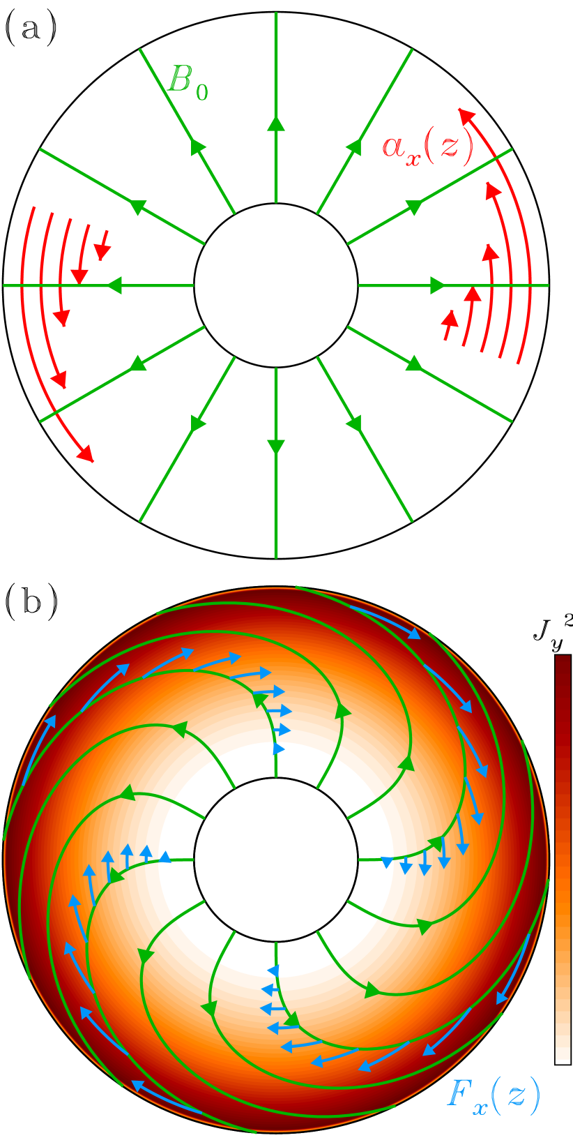
We express the axisymmetric magnetic field as
| (1) |
thus ensuring , and with setting the (fixed) strength of the radial magnetic component in the equatorial plane. The assumption of a radial background magnetic field allows us to write down the simplest model possible in the equatorial plane that captures the dynamics of Alfvén oscillations (Figure 1). A global aligned dipole lacks any radial component at the equator, and would require adding the latitudinal dimension to capture Alfvén oscillations. Of course, the true field geometry is likely to be more complicated than an aligned-dipole. A misaligned dipole or higher order multipoles would give radial field at the equator, and the actual magnetic field geometry could also be much more complex if a local dynamo operates in the atmospheric layer (Rogers & McElwaine, 2017; Dietrich et al., 2022). We adopt this simplified model as a starting point to capture the physics of the interaction of the temperature-dependent MD with magnetic torques.
The reduced MHD equations solved are thus:
| (2) |
| (3) |
| (4) | ||||
Equation (2) is the -component of the incompressible Navier-Stokes equation where is the density, and is the dynamic viscosity. The fluid motions are forced by an acceleration term
| (5) |
with the pressure measured in bars and setting the peak amplitude. This forcing is meant to capture the effects of angular momentum transfer to the equator from higher latitudes, for example by Rossby and Kelvin waves (Showman & Polvani, 2011).
Equation (3) is the -component of the induction equation with the temperature-dependent MD,
| (6) |
taken from Menou (2012a) and based on the results of Draine et al. (1983). The ionization fraction is obtained from the Saha equation (Rogers & Komacek, 2014) adopting solar abundances as given in Lodders (2010). Equation (4) is the heat transport equation with specific heat capacity and thermal conductivity
| (7) |
where is the Stefan-Boltzmann constant. The irradiation flux is
| (8) |
where is the flux from the host star incident on the atmosphere. In equations (7) and (8), is the Rosseland mean opacity (assumed constant), dominated by opacity at infrared-wavelengths, where most of the heat from the planet is emitted, while is the visible opacity, where the spectral flux of the host star peaks. The thermal conductivity is used to set the dynamic viscosity via an assumed Prandtl number :
| (9) |
The last two terms on the RHS of Equation (4) are the viscous () and ohmic () dissipation functions.
2.2 Boundary and initial conditions
We impose corotation with the core of the planet at the base, , and set vanishing mechanical stresses at the top boundary, . For the magnetic field, we set at the lower boundary, so as to ensure vanishing magnetic stress. At the outer boundary, we opt for a vacuum boundary condition, implying . For the temperature, we emulate a constant flux of energy coming from the core, , and a flux coming from the host star, , which is absorbed at depths controlled by the visible opacity, , as prescribed by Equation (8). We therefore set the inner temperature boundary condition at a constant flux corresponding to the sum of the two flux sources. The upper boundary is kept at a constant temperature .
We set the heat flux from the core as where K for all models, following M12, and then parametrize the thermal profile with and . For each choice of parameters, we set the values of , , and by comparing with the temperature profiles presented in M12 which are given as a function of . We solve the steady state form of Equation (4) with only the first three terms, i.e. we ignore any viscous and ohmic heating, jointly with the hydrostatic balance equation, using a ODE solver from SciPy111The function is solve_ivp from the integrate module. The documentation can be found at https://docs.scipy.org/doc/scipy/reference/generated/ scipy.integrate.solve_ivp.html, a Python package, using an explicit Runge-Kutta method of order 5. We then determine the values of and as a function of by fitting the temperature profiles shown in M12, and adopt a value m2 kg-1 for all models that reproduces the pressures at which the heat is deposited in M12.
The same initial conditions are used throughout: solid body rotation at the lower boundary rate , and purely radial magnetic field, i.e. and . The initial temperature profile is found jointly with the boundary conditions, as described in the previous paragraph, but we also let the solution from the ODE solver relax on our simulation grid. During this relaxation process, the barred variables in Equations (2)–(4) are allowed to adjust to the dissipationless steady-state temperature profile, but remain fixed thereafter. The initial MD is then simply given by Equation (6).
2.3 Numerical scheme
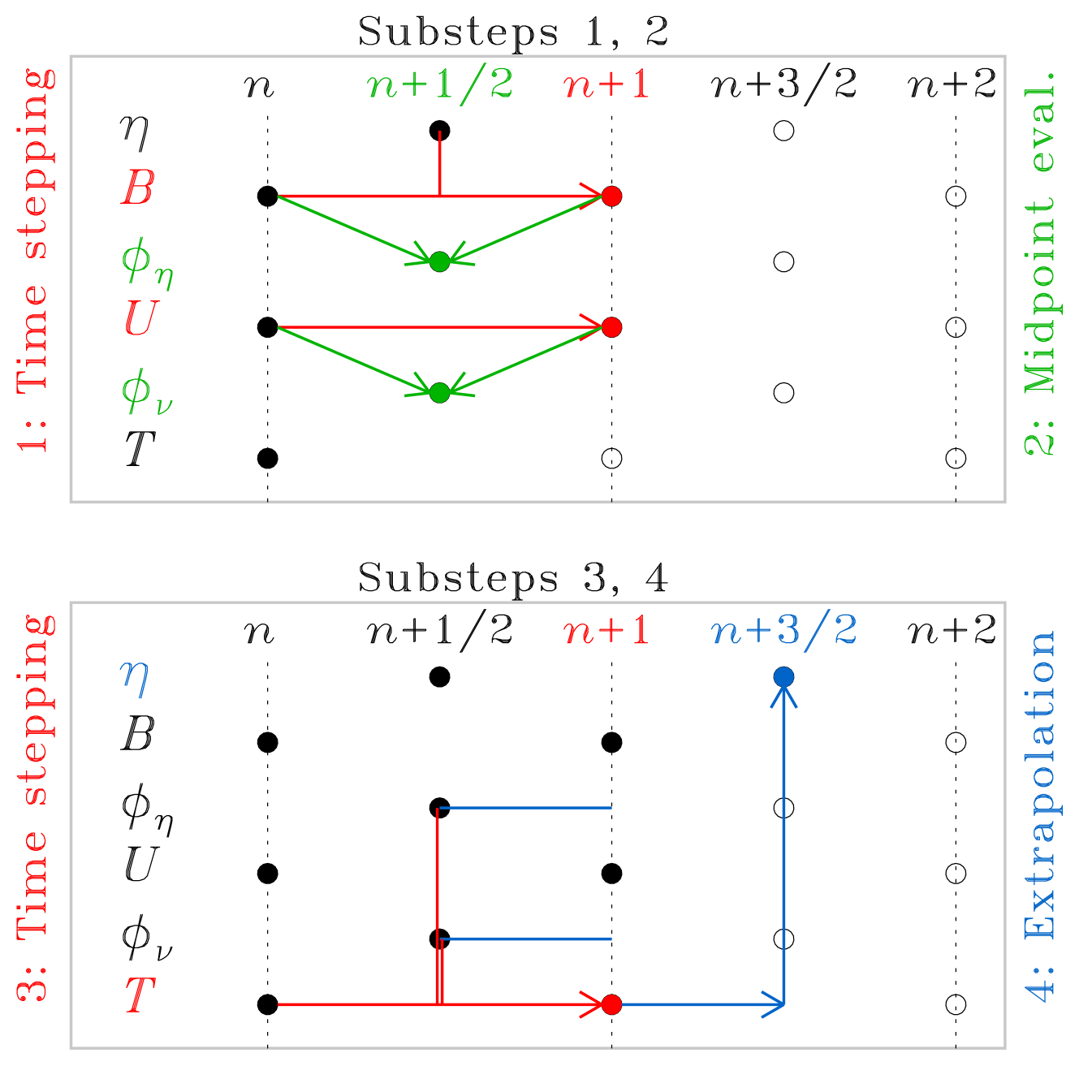
The numerical solution of Equations (2)–(4) requires the MD and dissipation functions , to be advanced in time. Because of the strongly nonlinear dependency of on , and of the dissipation functions and on flow and field gradients, simply evaluating these quantities at the current (known) time step when advancing Equations (2)–(4) to can lead to runaway numerical instabilities. Consequently, we opted to subdivide each time step into four substeps, as depicted schematically in Figure 2. In substep 1, we first advance the magnetic field and azimuthal velocity from time step to using a mid-point value for the MD, so as to ensure second-order accuracy in the spirit of centered finite differences. Equations (2) and (3) are advanced using a Crank-Nicolson scheme for the linear terms and Euler explicit for the nonlinear term. In substep 2, we use these newly calculated values of and at to do a mid-point () evaluation of the viscous and ohmic dissipation functions, namely the last two terms on the RHS of Equation (4). Substep 3 then advances from to via Crank-Nicolson, with mid-point evaluation of all source terms. The final substep 4 extrapolates at mid-step, from to , via a truncated Taylor series, i.e., at every grid point we write
| (10) |
the temperature derivative at being computed by evaluating the RHS of Equation (4) at for the linear terms, and for the dissipation functions. The MD at is then computed via Equation (6). This completes the time step, and the process can now repeat anew to advance from to .
Additionally, due to the boundary conditions imposed on the magnetic field, the ohmic heating is at its maximum at the top boundary. This raises issues, as we are keeping the temperature fixed at this end of the domain. To avoid buildup of a very thin thermal boundary layer, we have introduced a progressive ramp-down to zero of the viscous and ohmic heating terms in the outer 20% of the grid, following a dependency so as to maintain continuity of the second derivative in temperature. We have verified that this procedure does not affect significantly the TRI behavior or character of the resulting Alfvénic oscillations.
We use 100 grid points equally spaced in for all simulations. This was found to provide an acceptable compromise so as to adequately resolve boundary layers without becoming computationally prohibitive. Our time-stepping algorithm uses a constant time step which allows for suitable time resolution during the burst phase. To achieve this, we have used s for our simulations. We therefore need a few million time steps to complete a simulation. This represents around 2 core-days on a 4.90 GHz CPU.
2.4 Choice of parameter values
The free parameters for the simulations are the radial magnetic field strength, , the velocity forcing amplitude, , the thermal opacity, and the equilibrium temperature, . We opted to keep the Prandtl number small and constant throughout all simulations as ohmic heating is the focus of this study and HJ atmospheres are highly inviscid in our pressure range (Rogers & Komacek, 2014; Beltz et al., 2022). Table 1 lists the ranges in different parameter values that were used in our parameter space exploration.
| Parameters | Values |
|---|---|
| (G) | [10, 100] |
| (m s-2) | [0.0001, 0.01] |
| (m2 kg-1) | [0.0001, 0.001] |
| (K) | [1000, 1200] |
| Pr | [0.01] |
The choice of parameter values is guided by the results of H22. H22 presented a local model with a similar magnetic field and flow geometry to that considered here, that gave estimates for timescales and instability criterion as a function of pressure. Rewritten in dimensional units, the instability criterion that H22 derived is
| (11) |
where is the temperature-sensitivity of the MD, as defined in H22. We compute the instability criterion of Equation (11) across the domain, under the initial conditions, to ascertain in a first approximation which free parameter combinations satisfy Equation (11) and may result in an unstable system. We find that the H22 instability criterion is a good predictor of instability in our 1D model, and the TRI is robustly present. The fact that radial variations are included slightly changes the region of parameter space conducive to the TRI as compared to the local model results of H22. In addition, the behaviour is more complex since the local model parameters vary significantly across the radial direction, and velocity and magnetic field perturbations interact across a large pressure range.
3 Results
3.1 A representative simulation
We first examine in detail a representative simulation exhibiting recurrent oscillatory bursts triggered by the TRI. Figure 3 shows the time series of velocity, magnetic field perturbation, temperature and magnetic Reynolds number at the center of the domain through a series of seven recurrence cycles of oscillatory bursts (reminiscent of Figure 1 (c) of H22). The local magnetic Reynolds number is defined as , where is the local pressure scale height. The close-ups on the right hand side of Figure 3 focus on a single burst, and highlight the Alfvénic oscillations and their signature phase lag between velocity and magnetic field, as well as the exponential relationship between Rm and temperature coming from the ionization fraction, (c.f. Equation (6)). As pointed out by H22, the bursting behaviour is associated with a transition from during the build-up phase between bursts to during the oscillatory phase.
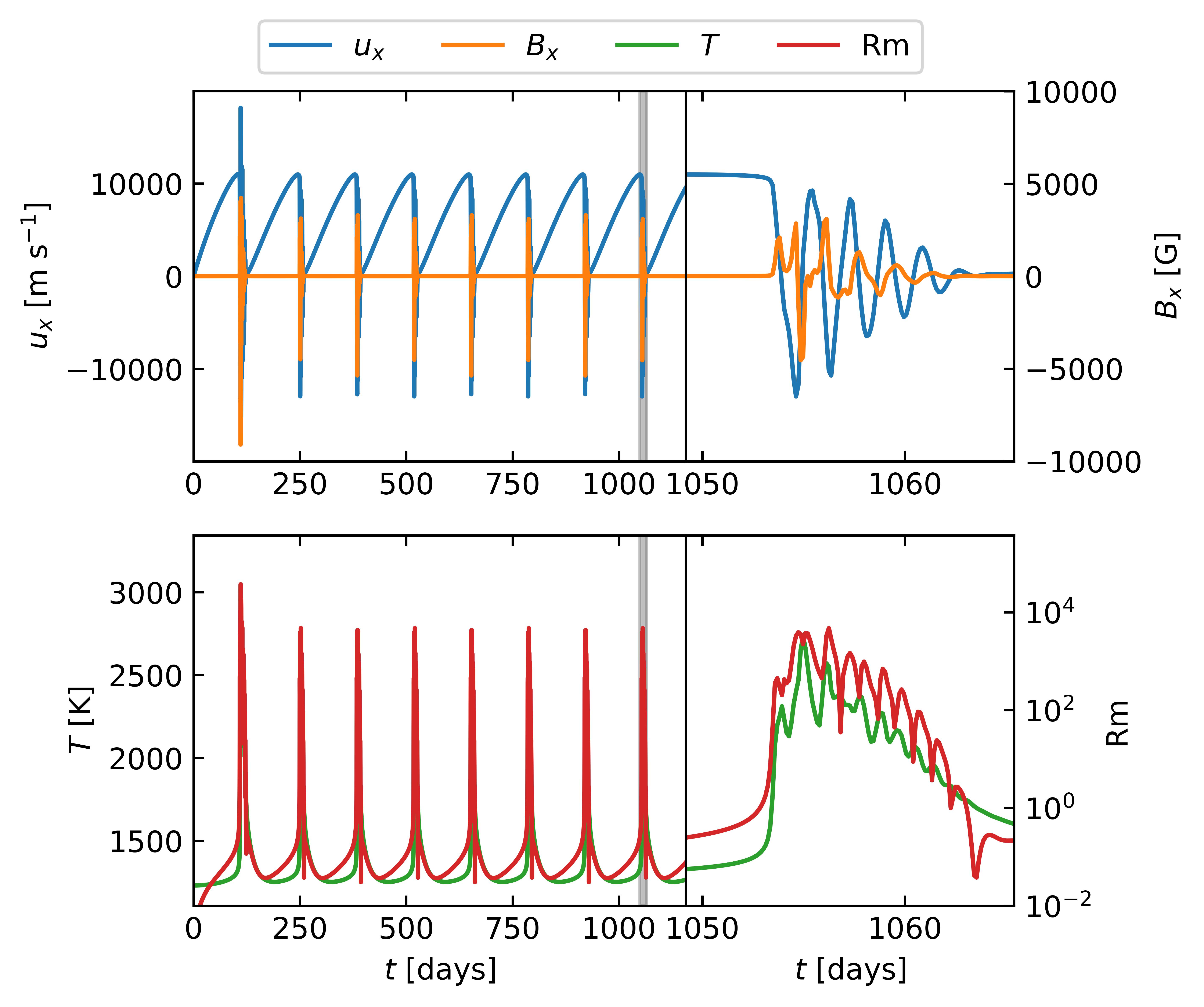
Figure 4 shows the phase space trajectory of the center point of the domain. The system starts at low velocity and low temperature and moves away from the plane as the velocity increases. The trajectory veers abruptly upwards once the critical temperature for TRI is reached. The initial runaway in temperature is as discussed by M12, but is halted, ultimately, by the dynamical back-reaction of the magnetic field on the flow, similar to the behavior seen in the local model of H22. After the oscillations have damped and the system cooled towards its equilibrium temperature, slow acceleration resumes, building up shear and inducing an azimuthal magnetic field, eventually triggering TRI and another oscillatory burst. A marked separation of timescale exists between the slow buildup phase, typically lasting weeks to months and in which the system spends most of its time, and the very rapid oscillatory burst and decay, spanning a few days.
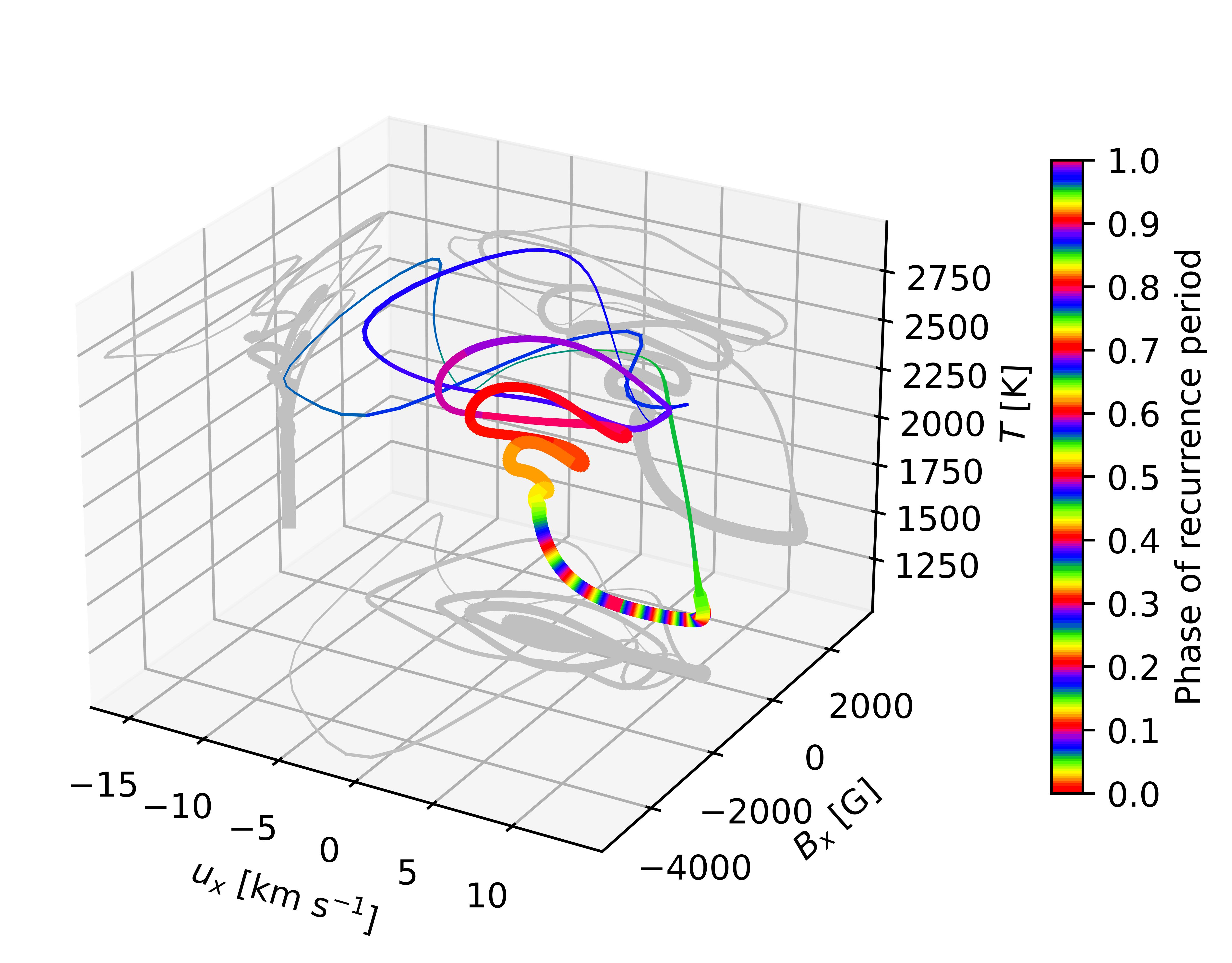
Figure 5 displays the temporal evolution of the – profile over one recurrence period. The profile changes rapidly once the TRI is triggered. The temperature at the higher pressures can exceed 3000 K at burst peak, as compared to 1300 K between bursts222In this example and other cases that reach peak temperatures close to , the temperature gradient is steep enough that convection would be expected to occur (not included in our calculation). However, the radial temperature gradient is likely enhanced by the fixed temperature outer boundary condition, and would be reduced with a more realistic outer boundary.. Such temperatures are expected at these pressures for equilibrium atmospheres with K.
3.2 Impact of the diffusivity gradient
We find that the (time-evolving) gradient of MD strongly influences the character of bursts and oscillations developing in the simulations. Figure 6 shows time series for three simulations differing only in their treatment of the diffusivity. In blue, we show a simulation based on the equations as presented in §2.1. In green, we show a simulation without the spatial gradient of the MD, i.e. the second term on the right hand side of Equation (3) has been artificially set to zero. In orange, we show a simulation in which the MD is time-independent, fixed to its initial profile.
While all three simulations show the same initial growth in velocity, the fixed diffusivity simulation (orange) simply grows to a steady-state, as in the local model of H22 and akin to most previous works treating magnetic effects as a drag force. The other two simulations, with time-varying MD, both develop oscillations, but bursting behavior only occurs if the (time-evolving) spatial MD gradient is retained. This can be traced to large spatial gradients of magnetic fields building up in the domain, enhancing dissipation and leading to very rapid rise of the temperature (the “burst”), subsequently transitioning to decaying Alfvén waves. These large magnetic gradients, building up in the lower part of the domain, can be seen in Figure 7 (top row), where time-evolving profiles of the velocity and magnetic field are shown during a single post-burst Alfvénic oscillation. Such strong gradients are absent in the simulation with the term artificially zeroed out (bottom row). The velocity and magnetic field also reaches much smaller values when the term is removed. For example, at the center of the domain the peak magnetic field is for the full simulation (Figure 3), but drops to when the term is removed, and for the fixed case.
With our geometrical setup and simplifications (i.e., and dd), the gradient term associated with the ohmic dissipation term in the -component of the induction equation becomes equivalent to , which is structurally akin to advection of by a “flow” . This is sometimes referred to as diamagnetic pumping. In our simulations the field is advected inwards, as is negative during build-up, while is positive. When the Alfvén oscillation starts, large gradients build up near the inner boundary, which lead to the very sharp increase in temperature due to a magnetic field varying very rapidly with depth, producing large amount of ohmic heating.
3.3 Region of parameter space exhibiting sustained oscillations and bursts
We find that certain choices of parameters are needed for sustained oscillations/bursts. For example, they occur only for equilibrium temperatures . This can be understood in terms of the magnetic Reynolds number, since a key characteristic of sustained oscillations is that the system needs to move between weak and strong flux freezing, i.e. between and (H22). Figure 8 shows an estimate of the magnetic Reynolds number in the – plane (for this estimate we assume a characteristic velocity of 5 km s-1, a rough average of the velocities in our oscillating solutions). Figure 8 suggests that the maximum equilibrium temperature allowing TRI-driven oscillatory bursts is around 1200 K, since hotter models have throughout the atmosphere (in agreement with Dietrich et al. (2022), who also find Rm at around K). Any system above this equilibrium temperature will be characterized by strong flux freezing from the beginning and will never be able to oscillate around . Conversely, colder atmospheres below around 1000 K may never reach as they do not experience enough heating, at least under reasonable velocity forcing.
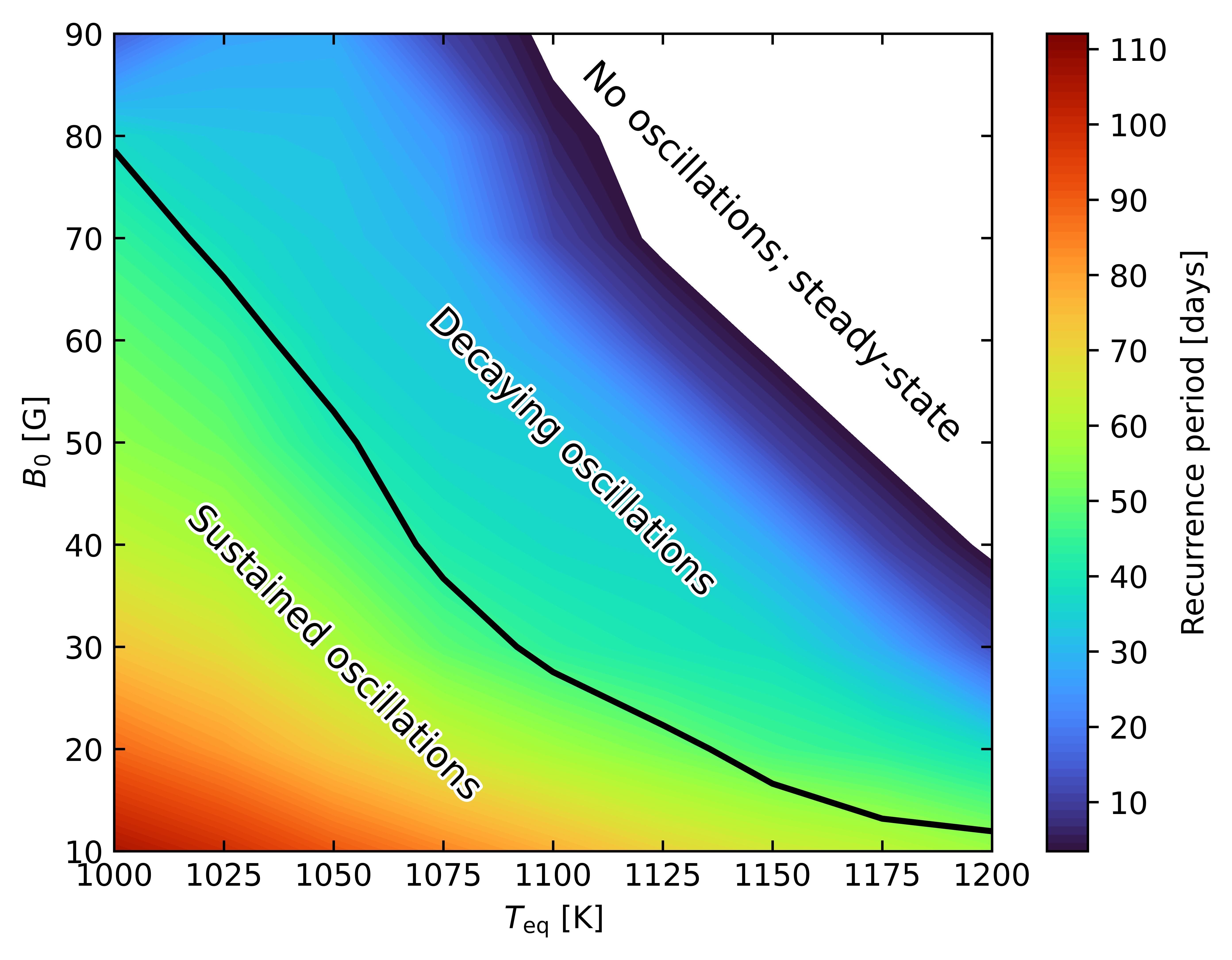
Figure 9 shows the different regimes in the – plane. We plot the recurrence period of the TRI, and take m s-1 and m2 kg-1. Instability and resulting oscillations are favored by weaker radial magnetic fields and lower equilibrium temperatures. The cooler temperatures are expected from Figure 8. Weaker radial fields require less forcing to be stretched azimuthally against the opposing Lorentz force, which is necessary to generate electrical currents and ohmic heating, the main heating contributor. As expected from H22, we have identified two different regimes in this figure: sustained oscillations, and systems that reach steady-state either by decaying Alfvénic oscillations or directly reach steady-state. We can see the recurrence period of the oscillations steadily shrinking as the systems approach the larger field and temperature values, even across the black line delimiting the two regimes.
3.4 Effect of thermal opacity variations
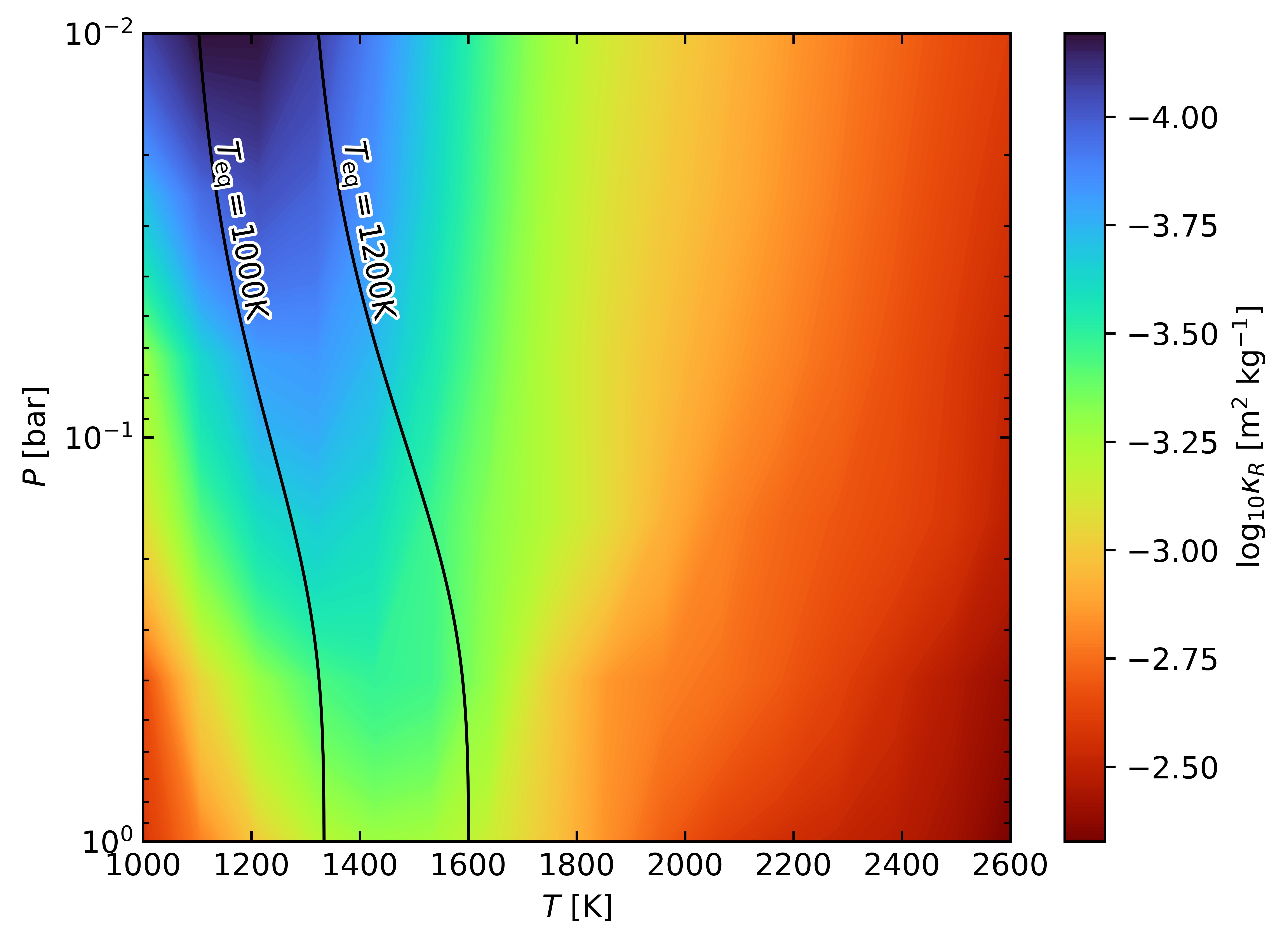
In the simulations presented so far, we assumed for simplicity that the opacity has a constant value. In fact, the opacity varies strongly throughout the atmosphere, as can be seen in Figure 10 where we plot the opacity in the – plane using the Freedman et al. (2008) opacity tables for dust free gas at solar metallicity. Comparing with the typical atmospheric temperature profiles shown in the Figure, we see that the opacity varies by an order of magnitude within our pressure range, and would also be changing locally during a burst as well as temperature changes.
To check the effect of opacity variations, we ran a simulation with a depth-dependent opacity profile, but still time independent, using the initial temperature profile to calculate as a function of depth. We used the following parameters: G, K, , . As a comparison baseline, we also ran a simulation with a constant thermal opacity of m2 kg-1 (), which corresponds to the opacity at around 0.5 bar for this equilibrium temperature. We find that the overall effect of the depth-dependent opacity is that the outer part of the envelope is not as insulating as with a constant opacity. Therefore, higher velocities are needed to reach the critical temperature, thus increasing the recurrence time of the TRI. Otherwise, the two simulations are qualitatively very similar.
HJs may have larger metallicities than solar (Welbanks et al., 2019). Freedman et al. (2008) also presents the values of the mean Rosseland opacity for a metallicity of . On average, for temperatures above 1000 K, the opacity with enhanced metallicity is larger by a factor of 1.7. Furthermore, the opacity presented by Freedman et al. (2008) are for dust and cloud free gas. However, the temperature range at which the TRI operates is in a regime where both dust and clouds are expected, which would enhance the opacity of the atmosphere. The opacity presented in Figure 10 is to be considered as a lower limit of the expected opacity in the atmosphere of a HJ.
Moreover, the opacity enters the calculation of the thermal conductivity (see Equation 7), which already varies with depth by a few orders of magnitude via its dependence on density and temperature. Introducing a depth dependence on opacity only adds another order of magnitude in the range of thermal conductivity (; Equation 7), and both and go down as pressure goes down). While not an insignificant variation, considering the uncertainties regarding this quantity in HJs atmospheres, the use of a constant thermal opacity is an acceptable approximation.
4 Discussion
We have presented a model of a forced azimuthal flow in the equatorial region of a HJ which captures the interplay between the dynamics associated with magnetic torques and thermal evolution due to ohmic heating. We find that self-sustained Alfvén oscillations are excited in the range of equilibrium temperatures – for magnetic field strengths of tens of Gauss (Figure 9). The oscillations occur in bursts, separated by long periods in which the magnetic field slowly winds up before a TRI is triggered (Figure 3). The subsequent increase in temperature increases the magnetic Reynolds number, the flow couples to the magnetic field, and oscillations occur. The need for the Rm to transition from below 1 to above 1 during the cycle sets the temperature range in which oscillations occur, ie. the temperature of the atmosphere needs to be such that Rm (Figure 8).
We find that the spatial gradients of MD strongly modify the radial profile of the Alfvén oscillations (Figure 6), including steepening of the magnetic field profile as perturbations propagate to higher pressure, enhancing dissipation at depth. Diamagnetic pumping like this has previously been found conducive to dynamo action, given a suitable alignment of and (Busse & Wicht, 1992; Pétrélis et al., 2016; Rogers & McElwaine, 2017) (although see also Rüdiger & Schultz 2022). Note however that in our model setup, dynamo action is precluded by Cowling’s theorem, since both the flow and magnetic field are axisymmetric. In their 3D simulations with a fixed spatially-varying electrical conductivity, Rogers & McElwaine (2017) found dynamo action for hotter HJs (nightside temperatures ). These hotter models would be expected to have large Rm (see Figure 8) enabling efficient dynamo action. At the lower values that we consider here, there could be recurrent bursts of dynamo activity, triggered by TRI.
Although we include the radial structure of the atmosphere, our model makes a number of simplifications. By restricting the geometry to the equatorial plane and assuming axisymmetry, we must impose an external forcing (; Equation 5) which models the day-night forcing and transport of angular momentum into the equatorial region by the global atmospheric flow. In addition, we have adopted the simplest possible field geometry (radial field) that supports Alfvén oscillations in our restricted geometry. Full global dynamical models that include the temperature-dependence of the MD will be needed to address these assumptions. We also have assumed constant viscosity and opacity in our model, and this could be relaxed in future work. Although the Prandtl number is small in planetary atmospheres, it would be interesting to study the effect of its time-dependence during the oscillation cycles. Including the temperature-dependence of opacity would give a more accurate determination of the properties of the oscillations (§3.4).
One impact of including additional physics in the model may be smaller oscillation amplitudes compared to those we find here. For example, we find that the zonal flows reach supersonic velocities during the burst for some choices of parameters. In the evolution shown in Figures 3 and 4, the peak velocity is above Mach 3. Supersonic velocities are not necessarily unreasonable, considering that they are observed in global hydrodynamical simulations (Cooper & Showman, 2005; Dobbs-Dixon & Lin, 2008; Showman et al., 2009; Rauscher & Menou, 2010; Lewis et al., 2010; Heng et al., 2011), where the maximum velocities can reach – at , and around at (Cooper & Showman, 2005; Rauscher & Menou, 2010). Dobbs-Dixon & Lin (2008) also note a peak speed of Mach 2 at the terminator in their simulations. However, we note that our model does not allow for processes, in particular the formation of shocks, that could limit supersonic flows. Similarly, additional physics could also intervene to prevent strong winding of the magnetic field, e.g. magnetic instabilities (Dietrich et al., 2022; Soriano-Guerrero et al., 2023). For example, Dietrich et al. (2022) estimate horizontal fields of (based on a – planetary field) could arise in KELT-9b from Alfvén oscillations, similar to the field strengths we find here (e.g. see Figure 3). However, they estimate that both Coriolis forces and Tayler instabilities would reduce this maximum field strength by about an order of magnitude. Finally, an improved treatment of both the outer and inner temperature boundaries is needed to more accurately determine the peak temperatures reached during the oscillations, in particular, allowing heat to propagate inwards to higher pressure and allowing the outer temperature to respond to changes in the outwards heat flux.
With the approximations underlying our model in mind, it is interesting to explore the possible implications for known hot jupiters. Figure 2 of Dietrich et al. (2022) shows estimated values of Rm as a function of for known hot jupiters. Large sources are often considered most interesting from the point of view of magnetism, since they have large Rm. Rogers (2017) found oscillations in wind velocities and hotspot displacement in simulations of the hot exoplanet HAT-P-7b (), and inferred a lower bound on the magnetic field strength needed to reproduce observed variability. Our results suggest that HJs with in the range - are interesting sources to model and to look at for variability driven by TRI. Possible sources in this temperature range are WASP-69 b, WASP-29 b and HAT-P-12 b on the colder side and WASP-39 b, WASP-34 b, and HD 189733 b on the hotter side333Equilibrium temperatures were obtained from the ExoAtmospheres database..
Our results suggest a number of possible observable features of TRI-driven oscillations. Typical recurrence times between bursts range from – months (Figure 9), and the periods of the oscillations are days. While the burst of oscillations is ongoing, ohmic heating raises the atmospheric temperature significantly (Figure 5), increasing the atmospheric scale height (by about a factor of 2 in the model shown in Figure 5). In addition, the oscillations involve periodic variations in velocity in the atmosphere, and could result in periodic displacements of the hot spot around the substellar point.
In summary, the results in this paper and in H22 highlight the need to include the temperature-dependence of MD in atmospheric models, and reveal a new regime of sustained oscillations around Rm . A set of 3D simulations that include the temperature-dependence of MD spanning a range of temperatures are needed. This would allow exploration of the full range of behavior, from drag at low Rm, self-sustained oscillations near Rm , to dynamo action or magnetic instabilities at large Rm, as well as to make predictions for observables that could be used to constrain the role of magnetism in HJ atmospheres.
This work was supported by the Natural Sciences and Engineering Research Council of Canada (NSERC) Discovery grants RGPIN-2023-03620 and RGPIN-2018-05278. R.H., A.C., and P.C. are members of the Centre de Recherche en Astrophysique du Québec (CRAQ).
References
- Armstrong et al. (2016) Armstrong, D. J., de Mooij, E., Barstow, J., et al. 2016, Nature Astronomy, 1, 0004, doi: 10.1038/s41550-016-0004
- Baraffe et al. (2003) Baraffe, I., Chabrier, G., Barman, T. S., Allard, F., & Hauschildt, P. H. 2003, A&A, 402, 701, doi: 10.1051/0004-6361:20030252
- Batygin & Stevenson (2010) Batygin, K., & Stevenson, D. J. 2010, ApJ, 714, L238, doi: 10.1088/2041-8205/714/2/L238
- Bell et al. (2019) Bell, T. J., Zhang, M., Cubillos, P. E., et al. 2019, MNRAS, 489, 1995, doi: 10.1093/mnras/stz2018
- Beltz et al. (2022) Beltz, H., Rauscher, E., Roman, M. T., & Guilliat, A. 2022, AJ, 163, 35, doi: 10.3847/1538-3881/ac3746
- Bodenheimer et al. (2003) Bodenheimer, P., Laughlin, G., & Lin, D. N. C. 2003, ApJ, 592, 555, doi: 10.1086/375565
- Bodenheimer et al. (2001) Bodenheimer, P., Lin, D. N. C., & Mardling, R. A. 2001, ApJ, 548, 466, doi: 10.1086/318667
- Busse & Wicht (1992) Busse, F. H., & Wicht, J. 1992, Geophysical and Astrophysical Fluid Dynamics, 64, 135, doi: 10.1080/03091929208228087
- Cooper & Showman (2005) Cooper, C. S., & Showman, A. P. 2005, ApJ, 629, L45, doi: 10.1086/444354
- Cowan et al. (2007) Cowan, N. B., Agol, E., & Charbonneau, D. 2007, MNRAS, 379, 641, doi: 10.1111/j.1365-2966.2007.11897.x
- Cowan et al. (2012) Cowan, N. B., Machalek, P., Croll, B., et al. 2012, ApJ, 747, 82, doi: 10.1088/0004-637X/747/1/82
- Crossfield et al. (2010) Crossfield, I. J. M., Hansen, B. M. S., Harrington, J., et al. 2010, ApJ, 723, 1436, doi: 10.1088/0004-637X/723/2/1436
- Dang et al. (2018) Dang, L., Cowan, N. B., Schwartz, J. C., et al. 2018, Nature Astronomy, 2, 220, doi: 10.1038/s41550-017-0351-6
- Davidson (2001) Davidson, P. A. 2001, An Introduction to Magnetohydrodynamics (Cambridge University Press)
- Dietrich et al. (2022) Dietrich, W., Kumar, S., Poser, A. J., et al. 2022, MNRAS, 517, 3113, doi: 10.1093/mnras/stac2849
- Dobbs-Dixon & Lin (2008) Dobbs-Dixon, I., & Lin, D. N. C. 2008, ApJ, 673, 513, doi: 10.1086/523786
- Draine et al. (1983) Draine, B. T., Roberge, W. G., & Dalgarno, A. 1983, ApJ, 264, 485, doi: 10.1086/160617
- Freedman et al. (2008) Freedman, R. S., Marley, M. S., & Lodders, K. 2008, ApJS, 174, 504, doi: 10.1086/521793
- Guillot & Showman (2002) Guillot, T., & Showman, A. P. 2002, A&A, 385, 156, doi: 10.1051/0004-6361:20011624
- Hardy et al. (2022) Hardy, R., Cumming, A., & Charbonneau, P. 2022, ApJ, 940, 123, doi: 10.3847/1538-4357/ac9bfc
- Heng et al. (2011) Heng, K., Menou, K., & Phillipps, P. J. 2011, MNRAS, 413, 2380, doi: 10.1111/j.1365-2966.2011.18315.x
- Hindle et al. (2019) Hindle, A. W., Bushby, P. J., & Rogers, T. M. 2019, ApJ, 872, L27, doi: 10.3847/2041-8213/ab05dd
- Hindle et al. (2021a) —. 2021a, ApJ, 916, L8, doi: 10.3847/2041-8213/ac0fec
- Hindle et al. (2021b) —. 2021b, ApJ, 922, 176, doi: 10.3847/1538-4357/ac0e2e
- Imamura et al. (2020) Imamura, T., Mitchell, J., Lebonnois, S., et al. 2020, Space Sci. Rev., 216, 87, doi: 10.1007/s11214-020-00703-9
- Jackson et al. (2019) Jackson, B., Adams, E., Sandidge, W., Kreyche, S., & Briggs, J. 2019, AJ, 157, 239, doi: 10.3847/1538-3881/ab1b30
- Kataria et al. (2016) Kataria, T., Sing, D. K., Lewis, N. K., et al. 2016, ApJ, 821, 9, doi: 10.3847/0004-637X/821/1/9
- Knutson et al. (2007) Knutson, H. A., Charbonneau, D., Allen, L. E., et al. 2007, Nature, 447, 183, doi: 10.1038/nature05782
- Knutson et al. (2009) Knutson, H. A., Charbonneau, D., Cowan, N. B., et al. 2009, ApJ, 690, 822, doi: 10.1088/0004-637X/690/1/822
- Knutson et al. (2012) Knutson, H. A., Lewis, N., Fortney, J. J., et al. 2012, ApJ, 754, 22, doi: 10.1088/0004-637X/754/1/22
- Komacek & Showman (2016) Komacek, T. D., & Showman, A. P. 2016, ApJ, 821, 16, doi: 10.3847/0004-637X/821/1/16
- Laughlin et al. (2005) Laughlin, G., Wolf, A., Vanmunster, T., et al. 2005, ApJ, 621, 1072, doi: 10.1086/427689
- Lewis et al. (2010) Lewis, N. K., Showman, A. P., Fortney, J. J., et al. 2010, ApJ, 720, 344, doi: 10.1088/0004-637X/720/1/344
- Lodders (2010) Lodders, K. 2010, Astrophysics and Space Science Proceedings, 16, 379, doi: 10.1007/978-3-642-10352-0_8
- Mayor & Queloz (1995) Mayor, M., & Queloz, D. 1995, Nature, 378, 355, doi: 10.1038/378355a0
- Menou (2012a) Menou, K. 2012a, ApJ, 745, 138, doi: 10.1088/0004-637X/745/2/138
- Menou (2012b) —. 2012b, ApJ, 754, L9, doi: 10.1088/2041-8205/754/1/L9
- Perna et al. (2010a) Perna, R., Menou, K., & Rauscher, E. 2010a, ApJ, 719, 1421, doi: 10.1088/0004-637X/719/2/1421
- Perna et al. (2010b) —. 2010b, ApJ, 724, 313, doi: 10.1088/0004-637X/724/1/313
- Pétrélis et al. (2016) Pétrélis, F., Alexakis, A., & Gissinger, C. 2016, Physical Review Letters, 116, 161102, doi: 10.1103/PhysRevLett.116.161102
- Rauscher & Menou (2010) Rauscher, E., & Menou, K. 2010, ApJ, 714, 1334, doi: 10.1088/0004-637X/714/2/1334
- Rauscher & Menou (2013) —. 2013, ApJ, 764, 103, doi: 10.1088/0004-637X/764/1/103
- Read & Lebonnois (2018) Read, P. L., & Lebonnois, S. 2018, Annual Review of Earth and Planetary Sciences, 46, 175, doi: 10.1146/annurev-earth-082517-010137
- Rogers (2017) Rogers, T. M. 2017, Nature Astronomy, 1, 0131, doi: 10.1038/s41550-017-0131
- Rogers & Komacek (2014) Rogers, T. M., & Komacek, T. D. 2014, ApJ, 794, 132, doi: 10.1088/0004-637X/794/2/132
- Rogers & McElwaine (2017) Rogers, T. M., & McElwaine, J. N. 2017, ApJ, 841, L26, doi: 10.3847/2041-8213/aa72da
- Rogers & Showman (2014) Rogers, T. M., & Showman, A. P. 2014, ApJ, 782, L4, doi: 10.1088/2041-8205/782/1/L4
- Rüdiger & Schultz (2022) Rüdiger, G., & Schultz, M. 2022, Astronomische Nachrichten, 343, e24011, doi: 10.1002/asna.20224011
- Schneider et al. (2011) Schneider, J., Dedieu, C., Le Sidaner, P., Savalle, R., & Zolotukhin, I. 2011, A&A, 532, A79, doi: 10.1051/0004-6361/201116713
- Showman et al. (2009) Showman, A. P., Fortney, J. J., Lian, Y., et al. 2009, ApJ, 699, 564, doi: 10.1088/0004-637X/699/1/564
- Showman & Guillot (2002) Showman, A. P., & Guillot, T. 2002, A&A, 385, 166, doi: 10.1051/0004-6361:20020101
- Showman & Polvani (2011) Showman, A. P., & Polvani, L. M. 2011, ApJ, 738, 71, doi: 10.1088/0004-637X/738/1/71
- Soriano-Guerrero et al. (2023) Soriano-Guerrero, C., Viganò, D., Perna, R., Akgün, T., & Palenzuela, C. 2023, arXiv e-prints, arXiv:2304.07066, doi: 10.48550/arXiv.2304.07066
- Thorngren et al. (2021) Thorngren, D. P., Fortney, J. J., Lopez, E. D., Berger, T. A., & Huber, D. 2021, ApJ, 909, L16, doi: 10.3847/2041-8213/abe86d
- von Essen et al. (2020) von Essen, C., Mallonn, M., Borre, C. C., et al. 2020, A&A, 639, A34, doi: 10.1051/0004-6361/202037905
- Welbanks et al. (2019) Welbanks, L., Madhusudhan, N., Allard, N. F., et al. 2019, ApJ, 887, L20, doi: 10.3847/2041-8213/ab5a89
- Zellem et al. (2014) Zellem, R. T., Lewis, N. K., Knutson, H. A., et al. 2014, ApJ, 790, 53, doi: 10.1088/0004-637X/790/1/53