Making Pre-trained Language Models both
Task-solvers and Self-calibrators
Abstract
Pre-trained language models (PLMs) serve as backbones for various real-world systems. For high-stake applications, it’s equally essential to have reasonable confidence estimations in predictions. While the vanilla confidence scores of PLMs can already be effectively utilized, PLMs consistently become overconfident in their wrong predictions, which is not desirable in practice. Previous work shows that introducing an extra calibration task can mitigate this issue. The basic idea involves acquiring additional data to train models in predicting the confidence of their initial predictions. However, it only demonstrates the feasibility of this kind of method, assuming that there are abundant extra available samples for the introduced calibration task. In this work, we consider the practical scenario that we need to effectively utilize training samples to make PLMs both task-solvers and self-calibrators. Three challenges are presented, including limited training samples, data imbalance, and distribution shifts. We first conduct pilot experiments to quantify various decisive factors in the calibration task. Based on the empirical analysis results, we propose a training algorithm LM-TOAST to tackle the challenges. Experimental results show that LM-TOAST can effectively utilize the training data to make PLMs have reasonable confidence estimations while maintaining the original task performance. Further, we consider three downstream applications, namely selective classification, adversarial defense, and model cascading, to show the practical usefulness of LM-TOAST. The code will be made public at https://github.com/Yangyi-Chen/LM-TOAST.
1 Introduction
We have witnessed the great success of pre-trained language models (PLMs) over the past few years in various tasks (Wang et al., 2019a, b). Nowadays, real-world natural language processing (NLP) systems are mostly built upon PLMs to effectively utilize their strong capacities (Bommasani et al., 2021; Han et al., 2021).
Beyond the performance evaluation, an essential requirement in high-stake applications for PLMs is to assign reasonable confidence to their predictions. This can enable the decision-makers to better handle the low-confident predictions, e.g., directly abstain to give predictions or transfer the input to human experts. The original predictive probability of PLMs can be effectively utilized for ranking predictions. This simple strategy can reasonably give relatively higher confidence to correct predictions compared to the wrong ones (Hendrycks et al., 2020a).
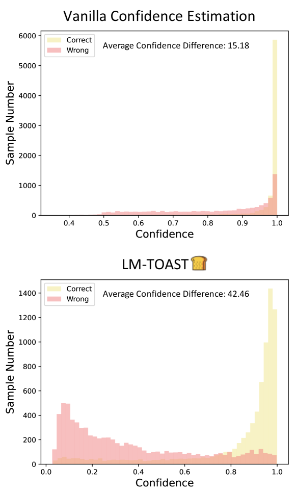
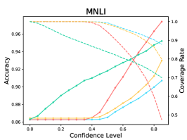
However, relying on the vanilla confidence scores cannot well distinguish between correct and wrong predictions. PLMs consistently assign high confidence in their predictions, no matter correct or not (Chen et al., 2022b). This results in a large number of wrong predictions distributed in the high-confident zone (see Figure 1). The direct undesirable consequence is the false acceptance of wrong but high-confident predictions. Besides, previous work avoids the issue of selecting a concrete confidence threshold by using hyper-parameter-free metrics (e.g., AUROC) in relevant tasks (e.g., selective classification). But in practice, the small gap between confidence in correct and wrong predictions may cause large performance variance due to the manually chosen threshold.
Existing work shows that an extra calibration task can be taken as a remedy (Chen et al., 2022b; Lin et al., 2022). The calibration task uses extra samples to train models to have reasonable confidence estimations. However, previous work considers ideal situations to demonstrate the feasibility, assuming access to a large number of unused labeled samples, typically from the validation set. In practice, the samples in the validation dataset may be too small to guarantee good calibration performance. Besides, relying on the validation samples for the calibration task training causes data leakage, which may result in unreliable performance estimation when adopting the validation dataset to choose hyper-parameters. In practice, we need to effectively utilize training samples for both the original and the calibration tasks training. Three challenges are presented:
-
•
Limited training samples: How to effectively utilize the training samples to increase the calibration task performance while maintaining the original task performance?
-
•
Data imbalance: Given PLMs’ high performance, the positive cases (correctly classified samples) significantly dominate the calibration training set, causing the data imbalance issue.
-
•
Distribution shifts: When deployed, PLMs are also expected to exhibit out-of-distribution (OOD) robustness, assigning reasonable confidence scores to OOD samples.
In this work, we motivate to make PLMs both task-solvers and self-calibrators in practical settings. We first conduct pilot experiments to quantify various decisive factors in the calibration task, including the number of training samples, the data imbalance ratio, and input “features” for the calibration task. Based on the empirical analysis, we propose a training algorithm LM-TOAST to tackle the challenges. We employ K-fold cross-annotation to generate the training data for the calibration task. Then we employ data down-sampling, adversarial data augmentation, and consistent training to tackle the challenges of data imbalance and distribution shifts. Note that LM-TOAST can be applied to all classification tasks to improve confidence estimations. Experimental results show that LM-TOAST can increase the discrimination between correct and wrong predictions, evidenced by the fine-grained order ranked by confidence and a sharp difference in average confidence.
Further, we show that the good self-calibration performance of LM-TOAST can be transferred to downstream applications. We consider three downstream tasks, including selective classification (Geifman and El-Yaniv, 2017), adversarial defense (Zhang et al., 2020), and model cascading (Varshney and Baral, 2022a). Experimental results demonstrate the practical significance of LM-TOAST in these applications.
2 Background
2.1 Task Formalization
In standard classification training, a model for the main task is trained on a given dataset to minimize the pre-defined classification loss. For the introduced calibration task, a new calibration dataset is generated from , where is the original sample in , is model’s prediction, and is the corresponding confidence score. The calibration task aims to predict the models’ confidence using the sample and the original prediction. The generation process of is one essential part of the calibration task. Lin et al. (2022) propose to deem accuracy on a batch of samples as the confidence for samples in this batch. In this work, we simplify this assumption and directly treat as a binary value, indicating whether the prediction is correct or not.
| Task | Template | Verbalizer | ||
|---|---|---|---|---|
| Main | It was <mask>, <input_sentence> | [bad, good, neutral] | ||
| Calibration |
|
[False, True] |

Once is generated, one can fit an extra model separately or conduct multi-task training using the original model to learn the calibration task111Due to the unified modeling approach proposed by Raffel et al. (2020), can be easily utilized as a mapping function .. In this work, we adopt the latter paradigm since no obvious performance difference is observed in previous work (Chen et al., 2022b). Specifically, we adopt the unified text-to-text paradigm and use T5 as the backbone model in this paper (Raffel et al., 2020). We use two sets of templates and verbalizers for the main task and the calibration task respectively (Liu et al., 2021). See Table 1 for an example used in the sentiment analysis task. Other templates and verbalizers selected are listed in Appendix B. The probability of the “True” class in the calibration task is deemed as PLMs’ confidence in their predictions. In testing, the original test set is used for evaluating both the original and the calibration tasks.
| Task | ID | OOD-1 | OOD-2 |
|---|---|---|---|
| Sentiment Analysis | Amazon | SST-5 | SemEval |
| Hate-speech Detection | Civil | Hate Speech | Implicit |
| Natural Language Inference | MNLI | HANS | ANLI |
2.2 Evaluation Setting
Evaluation metric.
We adopt two evaluation metrics to characterize whether PLMs assign reasonable confidence to testing samples that consist of correct and wrong predictions: (1) AUROC (Area Under the Receiver Operating Characteristic curve), which doesn’t require manually picking a threshold value (Davis and Goadrich, 2006). A better AUROC score indicates that correct predictions have relatively higher confidence scores than wrong ones; (2) Conf, which directly measures the average confidence difference between correct and wrong predictions. A higher Conf score indicates a better distinction between correct and wrong predictions from the confidence scores. Note we don’t use ECE (Naeini et al., 2015) since we mostly consider relative confidence scores in this work. See Fisch et al. (2022) for detailed elaborations.
Evaluation dataset.
For all experiments in this paper, we evaluate in both in-distribution (ID) and out-of-distribution (OOD) settings. We consider three classic tasks, including sentiment analysis, hate-speech detection, and natural language inference. We follow the same dataset chosen in Chen et al. (2022b) (see Table 2). The detailed descriptions and references are in Appendix A.

3 Pilot Experiments and Analysis
We conduct pilot experiments to quantify the influence of several decisive factors in the calibration task, which can help for a better design of various components in the training algorithm. Specifically, we consider the number of training samples, dataset imbalance, and input “features”. The concrete experimental settings are described in Appendix C.
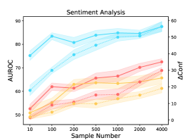
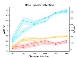
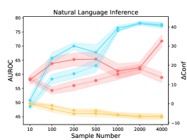
3.1 Number of Training Samples
We quantify the influence of available training samples in the calibration task (see Figure 2). We observe overall consistent trends in three different tasks across eight datasets. The results show the continued benefits of increasing the dataset size for the calibration task considering the AUROC and Conf scores. Surprisingly, the performance in OOD datasets can be improved by introducing more calibration training samples in ID datasets. This is different from the common belief that learning more in-domain knowledge may hurt the OOD robustness due to the reliance on spurious correlations (Radford et al., 2021). However, we note that there is an unnatural trend in the natural language inference task when ANLI is adopted as the OOD evaluation dataset. The reason may be partially attributed to the unique construction process of ANLI based on human-in-the-loop attacks.
3.2 Data Imbalance
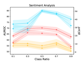
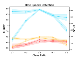
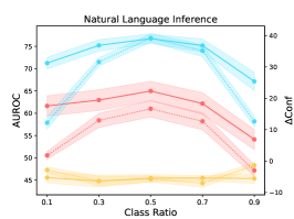
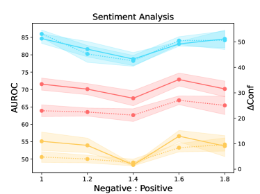
We vary the class ratios in the calibration training set to quantify the influence of data imbalance in the calibration task (see Figure 3). Note that there are two classes in the calibration training set, where the positive (negative) case indicates that the model’s original prediction is correct (wrong). The class ratio is defined as the fraction of negative-class samples in the whole dataset. We consistently observe inverted V-shapes considering all evaluation settings. Thus, we draw the conclusion that given a calibration dataset with a fixed number of samples, an exact balanced distribution of the two classes will mostly benefit the calibration task.
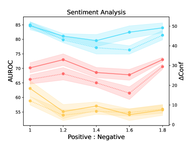
Further, we consider a more practical question faced in our algorithm: Given limited training samples in one class, what is the influence of continuing to increase the training samples in the other class? We conduct two rounds of experiments. For each round, we fix the samples in one class and continue to increase the samples in the other class. The results are shown in Figure 7. We observe roughly V-shapes in both two rounds. Also, we carefully observe the two ends of the V shapes and find that these two dataset scaling processes can hardly bring a positive effect on PLMs’ calibration performance. Thus, given limited available training samples, the optimal strategy is to keep the dataset with an exact balanced distribution of two classes even if we have extra data because we cannot precisely predict how many samples we should add to one single class to improve the calibration performance.
3.3 Input “Features”
Recall from Sec. 2.1 that two “features” exist in each calibration training sample , including the original sample and the model’s original prediction . We ablate the influence of these two “features” (see Table 3). We observe the dominant effect of information extracted from the original sample . While still lagging behind the calibration performance when using all features, only relying on the original sample for the prediction can achieve descent performance in most cases.
The experimental results can further inform us of the essence of the calibration task. Given the descent performance when only using the original samples as the input features, PLMs mostly are performing the task of determining the difficulty of each sample, where hard (easy) samples will be assigned low (high) confidence scores. The potential major function PLMs learn in the calibration task training may be inducing which kinds of features in the texts they cannot handle well. In this work, we motivate to exploit the calibration methods, and further exploration and utilization of the inner mechanism are left for future work.
| Amazon | Dataset | Amazon | SST-5 | SemEval | |||
|---|---|---|---|---|---|---|---|
| Method | AUROC | Conf | AUROC | Conf | AUROC | Conf | |
| All Features | 89.44 (0.08) | 73.96 (0.35) | 61.95 (0.16) | 28.94 (0.82) | 73.70 (1.18) | 28.65 (0.57) | |
| w/o Prediction | 84.12 (0.49) | 64.81 (0.87) | 59.47 (1.04) | 24.46 (0.24) | 68.15 (1.42) | 22.46 (2.67) | |
| w/o Sample | 70.06 (1.67) | 3.93 (1.07) | 57.22 (3.31) | 1.16 (0.55) | 59.19 (0.94) | 1.42 (0.37) | |
| Civil | Dataset | Civil | Hate Speech | Implicit | |||
| Method | AUROC | Conf | AUROC | Conf | AUROC | Conf | |
| All Features | 86.98 (5.00) | 59.30 (0.10) | 60.44 (0.39) | 11.18 (2.28) | 64.16 (1.98) | 21.05 (2.95) | |
| w/o Prediction | 83.89 (2.51) | 52.74 (3.83) | 61.83 (4.52) | 14.90 (8.28) | 63.93 (0.32) | 20.96 (0.22) | |
| w/o Sample | 5.18 (0.20) | -3.5 (2.39) | 55.73 (0.79) | 4.35 (0.27) | 37.02 (0.21) | -1.02 (0.71) | |
| MNLI | Dataset | MNLI | HANS | ANLI | |||
| Method | AUROC | Conf | AUROC | Conf | AUROC | Conf | |
| All Features | 78.80 (0.89) | 42.64 (0.58) | 67.90 (3.16) | 24.11 (6.55) | 44.31 (0.30) | -6.95 (0.99) | |
| w/o Prediction | 79.24 (0.31) | 44.94 (0.42) | 60.22 (2.11) | 14.11 (4.32) | 43.99 (0.23) | -8.05 (1.33) | |
| w/o Sample | 39.19 (0.89) | 0 (0.11) | 39.12 (0.34) | 0 (0.09) | 51.28 (0.24) | 0 (0.01) | |
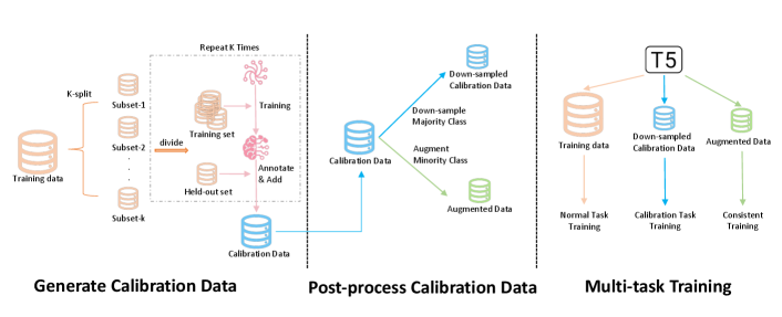
 , consisting of three separate stages, namely generating calibration data, post-processing calibration data, and multi-task training.
4 Method
Based on our empirical analysis summarized in Appendix C, we motivate a practical training algorithm to make PLMs both Task-sOlvers And Self-calibraTors (LM-TOAST![]() ).
LM-TOAST can be divided into three stages (see Figure 4):
(1) Generate calibration training data from the given training dataset;
(2) Post-process generated calibration training data;
(3) Multi-task training using the original training data and the processed calibration training data.
We follow the notations in Sec. 2.1.
).
LM-TOAST can be divided into three stages (see Figure 4):
(1) Generate calibration training data from the given training dataset;
(2) Post-process generated calibration training data;
(3) Multi-task training using the original training data and the processed calibration training data.
We follow the notations in Sec. 2.1.
Generate calibration training data.
We propose the K-fold cross-annotation to generate the calibration dataset from the original training samples. We first split the original training dataset into K subsets equally, and perform K-rounds annotation. For each round, we leave one subset out and train the model on the remaining K-1 subsets. Then we use the trained model to annotate the held-out set. Specifically, for each sample in the held-out set, we obtain the model’s prediction and compare it with the golden label. A binary annotated label is obtained, indicating whether the prediction is correct or not. After K-rounds annotation, we can generate a calibration training dataset with the size equal to the original training dataset’s size. We empirically set K=2 in LM-TOAST to avoid hyper-parameter searching. We justify this setting in the further analysis of LM-TOAST (see Appendix D). Note that due to the strong capacity of PLMs, there exists a significant data imbalance issue in , where positive cases dominate the distribution. Thus, post-processing the generated calibration data is needed to make full use of .
Post-process generated calibration training data.
Data imbalance is a long-standing research problem in machine learning. We visit existing methods for our calibration task. According to our pilot exploration, we adopt two strategies tailored for our task, namely down-sampling the majority class and performing data augmentation on the minority class. For the former one, we simply down-sample the majority class to achieve the exact balance of two classes in the calibration training dataset. For data augmentation on the minority class, we employ textual transformation methods (Wei and Zou, 2019; Li et al., 2021a) to generate the constructed set that contains augmented negative samples:
| (1) |
where is the textual transformation method. Specifically, we consider the following methods and choose them randomly: (1) Synonym substitution: Exploiting WordNet (Miller, 1995) to substitute words in original samples with their synonyms; (2) Random insertion: Randomly inserting or repeating some words in original samples; (3) Random swap: Randomly swapping the order of adjacent words in original samples; (4) Random deletion: Randomly deleting some words in original samples.
Multi-task training.
After the post-processing, we currently possess the original training set , the generated and then down-sampled calibration training set , the constructed set containing augmented negative samples. We find that directly mixing and for the calibration task training has minimal or negative effects on the calibration performance. The bottleneck substantially lies in the diversity and quality of the augmented samples, which is the central problem in textual data augmentation research.
Thus, we treat and separately and adopt different training strategies. In high-quality , we conduct normal classification training:
| (2) |
where CE is the cross-entropy loss. For easy reference, is the original sample in D, is model’s original prediction, and is a binary value, indicating whether the prediction is correct or not. In that contains noise, a robust training algorithm is needed to effectively utilize the augmented samples. Specifically, we draw inspirations from Miyato et al. (2017) that consider the problem of textual adversarial training. They propose to use consistent training to enforce that the predictive probability of the original input is the same as that of the corresponding input with gradient-based perturbations added in the embedding layer. Similarly, we propose to constrain the predictive probability of the original samples and corresponding augmented samples:
| (3) |
where KL measures the Kullback–Leibler divergence between two distributions. Considering the original task, we conduct multi-task training to minimize the loss :
| (4) |
| (5) |
where CE is the cross-entropy loss, is the loss of the original task, and is a hyper-parameter to control the influence of the consistent loss. We empirically set to 0.1 in LM-TOAST to avoid hyper-parameter searching. We justify this setting in the further analysis of LM-TOAST (see Appendix D).
5 Experiments
We conduct experiments to demonstrate the effectiveness of LM-TOAST in confidence estimations. We run all experiments three times and report both the average performance and the standard variance.
5.1 Baseline Methods
We adopt three baseline methods for confidence estimations: (1) Vanilla: Use the original predictive probability as the confidence estimation; (2) Temperature Scaling (TS): Apply the temperature scaling method to calibrate PLMs’ confidence scores (Guo et al., 2017); (3) Label Smoothing (LS): Apply label smoothing to prevent PLMs from becoming overconfident in their predictions (Szegedy et al., 2016).
5.2 Results of Calibration Performance
| Amazon | Dataset | Amazon | SST-5 | SemEval | |||
|---|---|---|---|---|---|---|---|
| Method | AUROC | Conf | AUROC | Conf | AUROC | Conf | |
| Vanilla | 85.80 (0.45) | 15.18 (0.33) | 79.14 (0.83) | 16.56 (0.78) | 71.68 (0.93) | 12.68 (0.59) | |
| TS | 85.80 (0.45) | 16.85 (0.59) | 79.14 (0.83) | 10.63 (0.34) | 71.68 (0.93) | 8.07 (0.64) | |
| LS | 81.93 (2.77) | 13.81 (0.83) | 76.81 (1.41) | 13.45 (0.99) | 70.52 (1.26) | 10.81 (0.90) | |
| LM-TOAST |
87.44 (1.12) | 42.46 (3.03) | 79.32 (1.09) | 26.37 (1.04) | 73.17 (2.36) | 20.21 (1.70) | |
| Civil | Dataset | Civil | Hate Speech | Implicit | |||
| Method | AUROC | Conf | AUROC | Conf | AUROC | Conf | |
| Vanilla | 90.33 (0.99) | 14.23 (0.09) | 62.80 (0.55) | 2.74 (0.64) | 65.99 (1.22) | 3.63 (1.19) | |
| TS | 90.33 (0.99) | 22.71 (0.46) | 62.80 (0.55) | 5.60 (0.27) | 65.99 (1.22) | 7.25 (0.23) | |
| LS | 91.15 (0.11) | 11.59 (0.32) | 62.17 (0.22) | 2.08 (0.33) | 63.92 (0.13) | 3.30 (0.34) | |
| LM-TOAST |
92.01 (0.14) | 51.38 (0.24) | 65.55 (1.76) | 12.57 (2.47) | 65.99 (0.12) | 17.29 (0.30) | |
| MNLI | Dataset | MNLI | HANS | ANLI | |||
| Method | AUROC | Conf | AUROC | Conf | AUROC | Conf | |
| Vanilla | 82.08 (0.43) | 12.25 (0.19) | 51.14 (1.68) | 2.59 (0.52) | 44.14 (0.31) | -2.31 (0.06) | |
| TS | 82.08 (0.43) | 18.30 (0.32) | 51.14 (1.68) | -1.87 (0.70) | 44.14 (0.31) | -2.89 (0.13) | |
| LS | 80.51 (0.14) | 10.12 (0.39) | 46.52 (2.32) | 0.53 (0.80) | 43.07 (0.32) | -2.91 (0.92) | |
| LM-TOAST |
82.74 (0.49) | 33.53 (1.40) | 60.60 (4.34) | 11.19 (3.81) | 43.97 (0.62) | -6.69 (0.70) | |
The experimental results are listed in Table 4. We observe that LM-TOAST achieves overall better calibration performance. For fine-grained confidence ranking of correct and wrong predictions (AUROC), LM-TOAST improves the discrimination of wrong predictions by assigning them with relatively lower confidence. Also, we note that vanilla confidence can already be adopted for effectively detecting wrong predictions, consistent with previous work (Hendrycks et al., 2020a).
However, as shown in Figure 1, there is no distinguished confidence gap between confidence scores on correct and wrong predictions. This results in many high-confident wrong predictions, which is undesirable since false acceptance may happen in reality. Besides, previous work regarding the utilization of vanilla confidence scores (e.g., selective classification (Kamath et al., 2020)) overlooks this issue since the selected metric mostly doesn’t need a chosen threshold (e.g., AUROC). But in practice, a small confidence gap between correct and wrong predictions makes it hard for practitioners to manually select a concrete threshold and may cause large performance variance. Thus, it’s also essential to measure the confidence gap between correct and wrong predictions. We show that LM-TOAST can significantly increase this gap, in both ID and OOD settings. One exception is still the ANLI dataset. We refer to Sec. 3.1 for our explanation.
Due to space limits, we present further analysis of LM-TOAST in Appendix D, including the ablation study of each component and the influence of the hyper-parameter K in the cross-annotation.
6 Applications
We consider applying LM-TOAST for three tasks, namely selective classification (Geifman and El-Yaniv, 2017), adversarial defense (Zhang et al., 2020), and model cascading (Varshney et al., 2022). The baseline methods are the same as in Sec. 5
6.1 Selective Classification
Selective classification provides systems with an extra reject option. It plays an essential role in high-stake application scenarios (e.g., fake news detection) since the systems can trade off the prediction coverage for better prediction performance. Once PLMs’ confidence scores on predictions are lower than the pre-defined threshold, the systems may reject PLMs’ predictions and transfer the inputs to human experts. Thus, the task performance can be improved by clearly distinguishing the wrong predictions. The evaluation settings are described in Appendix F.
Experimental results.
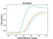
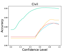
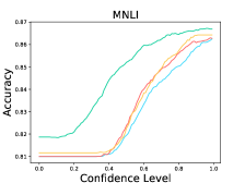
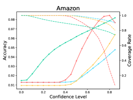
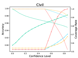
The results are listed in Table 9. We observe that LM-TOAST overall achieves both the minimum risk averaging over various coverage measured by AUROCrisk and the maximum coverage for the desired risk level. To further show the advantage of LM-TOAST, we plot the accuracy versus confidence level (a.k.a., threshold) curves for three ID datasets (see Figure 8). The predictions with confidence scores lower than the confidence level will be rejected. We observe that LM-TOAST can steadily increase performance when the confidence level keeps getting larger. Besides, LM-TOAST achieves an overall better balance between accuracy and coverage rate. On the contrary, while using TS can achieve good performance in high confidence levels, the coverage rate is very low (near 0 on Amazon).

6.2 Adversarial Defense
| Dataset | PWWS | TextBugger | BERT-Attack | HotFlip | ROCKET | |||||
|---|---|---|---|---|---|---|---|---|---|---|
| Method | AUROC | Conf | AUROC | Conf | AUROC | Conf | AUROC | Conf | AUROC | Conf |
| Vanilla | 74.91 | 15.66 | 79.11 | 17.68 | 81.13 | 21.57 | 83.54 | 19.01 | 77.23 | 14.24 |
| TS | 74.91 | 10.79 | 79.11 | 12.53 | 81.13 | 13.79 | 83.54 | 14.19 | 77.23 | 11.33 |
| LS | 71.10 | 10.28 | 74.53 | 11.18 | 76.51 | 12.31 | 78.69 | 12.15 | 64.24 | 9.26 |
| LM-TOAST |
84.64 | 42.66 | 86.01 | 45.75 | 84.59 | 45.08 | 87.96 | 49.56 | 85.83 | 42.78 |
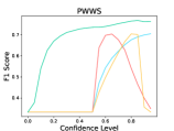
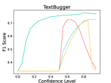
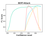
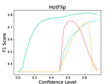
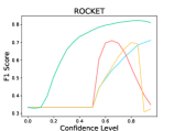
For PLMs deployed for security-relevant applications (e.g., hate-speech detection), malicious agents may construct adversarial samples to mislead PLMs’ predictions. Essentially, the attack methods introduce noise to the original samples, which may result in various degrees of distribution shifts (Zhang et al., 2015; Yuan et al., 2021; Wang et al., 2022). Thus, adversarial sample detection can be treated as a special kind of OOD detection problem, and the confidence scores can be exploited. The intuition is that PLMs’ confidence scores may be lower in adversarial OOD samples compared to ID ones. The evaluation settings are described in Appendix F. Basically, a sample is considered adversarial when the predictive probability is below a certain threshold.
Experimental results.
The results are listed in Table 5. We observe that LM-TOAST achieves significantly better performance in detecting adversarial inputs. Further, we sample 1,000 sentences from the ID dataset and mix them with adversarial samples. We measure the Macro-F1 score at various confidence levels considering five attack methods (see Figure 5). The samples with confidence scores lower than the confidence level will be treated as adversarial samples. We observe that LM-TOAST reacts more actively to the confidence threshold chosen, and consistently achieves better detection results across all thresholds.
| Dataset | Amazon | Civil | MNLI |
|---|---|---|---|
| Method | AUROC | AUROC | AUROC |
| Vanilla | 88.24 | 86.55 | 81.96 |
| TS | 88.37 | 86.60 | 82.21 |
| LS | 88.34 | 86.62 | 82.30 |
| LM-TOAST |
89.50 | 88.54 | 83.93 |

6.3 Model Cascading
Model cascading systems build a model pool consisting of PLMs with various scales (Varshney and Baral, 2022a). Given input samples in the inference time, smaller models can be first adopted for predictions. If the predictive confidence scores are relatively lower, the system can transfer samples to larger models, which will take more time to solve but with more accuracy. The basic intuition is that smaller models can already give correct predictions in most cases, and larger models are only needed to be adopted when solving some difficult samples. In this way, model cascading systems can significantly improve the efficiency in the inference time. The evaluation settings are described in Appendix F.
Experimental results.
The results are listed in Table 6. LM-TOAST achieves better performance on three datasets. Thus, incorporating the confidence estimations computed by LM-TOAST can improve the efficiency and performance of the cascading systems. We also show the accuracy versus the confidence level curves in Figure 6. The samples with confidence scores from the small model lower than the confidence level will be transferred to the large model for prediction. LM-TOAST still exhibits the benefit of reacting dynamically with the confidence changing and consistently achieves better performance considering all thresholds.
7 Related Work
Calibration methods.
Typically, calibration methods rely on human intuitions or posterior adjustments to make the confidence estimations more accurate. Data augmentation (Hendrycks et al., 2020b; Wang et al., 2021) and model ensemble (Gal and Ghahramani, 2016; Lakshminarayanan et al., 2017) have been empirically proven to be successful in computer vision. However, they cannot bring the same benefits in NLP according to the empirical study in Chen et al. (2022b). So we don’t consider them as baseline methods for comparison in this work, and two empirically effective methods are adopted. Temperature scaling (Platt et al., 1999; Guo et al., 2017) readjusts the output logits in a posterior way according to the calibration performance on a held-out set. Label smoothing (Szegedy et al., 2016) imposes a confidence regularization during the training process, discouraging models from being overconfident in their predictions.
Recently, there is an emergent trend in NLP, motivating to directly collect data for training models to have reasonable confidence estimations. Kadavath et al. (2022) assume that the last hidden states of PLMs contain the uncertainty information, and directly apply a multi-layer perceptron on them to perform confidence estimations. Lin et al. (2022) also show that PLMs can be directly trained to give their confidence estimations by words. These two methods are proven to be successful in significantly reducing the overconfidence issue and are further extended to exploit the potential in this kind of methods (Chen et al., 2022b). Existing work demonstrates the feasibility and potential of this kind of method in ideal experimental settings that enough training data is given for the calibration task. We further consider the practical setting and propose an effective method in this work.
Applications.
The confidence scores have been widely utilized for various applications. A bunch of active learning methods relies on models’ confidence to select the most informative samples to annotate (Zhang et al., 2022; Schröder et al., 2022). Models’ confidence can also be directly utilized for OOD and misclassification detection (Hendrycks and Gimpel, 2017; Hendrycks et al., 2020a). Following the same intuition, selective prediction can be applied to improve the system performance by filtering out low-confident predictions (Geifman and El-Yaniv, 2017; Kamath et al., 2020; Varshney et al., 2022). Moreover, an alternative strategy is adopting the model cascading systems, transferring the low-confident inputs to models with higher capacities (Li et al., 2021b; Varshney and Baral, 2022a). This can achieve better performance and efficiency of the whole system.
8 Conclusion
We present the task-agnostic LM-TOAST to make PLMs have reasonable confidence estimations while maintaining the original task performance. We also show that its good self-calibration can be transferred to downstream applications.
Limitations and Future Work
We acknowledge the limitations of LM-TOAST in few-shot calibration training. From our pilot experiments in Sec. 3.1, we observe that a significant amount of data points are needed for the calibration task training. In LM-TOAST, we effectively utilize the whole training set for the calibration task. Some learning paradigms assume only a small number of annotated samples at first, which limits the effectiveness of LM-TOAST. For example, in active learning (Zhang et al., 2022; Schröder et al., 2022), only a very small number of samples are available at the beginning most of the time, and models need to rely on them to find informative unlabeled samples to annotate. The vanilla confidence scores can be effectively utilized in this setting. However, LM-TOAST may not learn the calibration task well given very limited samples, resulting in poor performance in searching informative samples. We plan to investigate the calibration task in the few-shot setting and bring out the potential in LM-TOAST to make it suitable for more tasks.
References
- Bommasani et al. (2021) Rishi Bommasani, Drew A. Hudson, Ehsan Adeli, Russ Altman, Simran Arora, Sydney von Arx, Michael S. Bernstein, Jeannette Bohg, Antoine Bosselut, Emma Brunskill, Erik Brynjolfsson, Shyamal Buch, Dallas Card, Rodrigo Castellon, Niladri S. Chatterji, Annie S. Chen, Kathleen Creel, Jared Quincy Davis, Dorottya Demszky, Chris Donahue, Moussa Doumbouya, Esin Durmus, Stefano Ermon, John Etchemendy, Kawin Ethayarajh, Li Fei-Fei, Chelsea Finn, Trevor Gale, Lauren Gillespie, Karan Goel, Noah D. Goodman, Shelby Grossman, Neel Guha, Tatsunori Hashimoto, Peter Henderson, John Hewitt, Daniel E. Ho, Jenny Hong, Kyle Hsu, Jing Huang, Thomas Icard, Saahil Jain, Dan Jurafsky, Pratyusha Kalluri, Siddharth Karamcheti, Geoff Keeling, Fereshte Khani, Omar Khattab, Pang Wei Koh, Mark S. Krass, Ranjay Krishna, Rohith Kuditipudi, and et al. 2021. On the opportunities and risks of foundation models. CoRR, abs/2108.07258.
- Chen et al. (2022a) Yangyi Chen, Hongcheng Gao, Ganqu Cui, Fanchao Qi, Longtao Huang, Zhiyuan Liu, and Maosong Sun. 2022a. Why should adversarial perturbations be imperceptible? rethink the research paradigm in adversarial NLP. CoRR, abs/2210.10683.
- Chen et al. (2022b) Yangyi Chen, Lifan Yuan, Ganqu Cui, Zhiyuan Liu, and Heng Ji. 2022b. A close look into the calibration of pre-trained language models. CoRR, abs/2211.00151.
- Cui et al. (2022) Ganqu Cui, Lifan Yuan, Bingxiang He, Yangyi Chen, Zhiyuan Liu, and Maosong Sun. 2022. A unified evaluation of textual backdoor learning: Frameworks and benchmarks. In NeurIPS.
- Davis and Goadrich (2006) Jesse Davis and Mark Goadrich. 2006. The relationship between precision-recall and ROC curves. In Machine Learning, Proceedings of the Twenty-Third International Conference (ICML 2006), Pittsburgh, Pennsylvania, USA, June 25-29, 2006, volume 148 of ACM International Conference Proceeding Series, pages 233–240. ACM.
- de Gibert et al. (2018) Ona de Gibert, Naiara Perez, Aitor García-Pablos, and Montse Cuadros. 2018. Hate speech dataset from a white supremacy forum. In Proceedings of the 2nd Workshop on Abusive Language Online (ALW2), pages 11–20, Brussels, Belgium. Association for Computational Linguistics.
- Ebrahimi et al. (2018) Javid Ebrahimi, Anyi Rao, Daniel Lowd, and Dejing Dou. 2018. Hotflip: White-box adversarial examples for text classification. In Proceedings of the 56th Annual Meeting of the Association for Computational Linguistics, ACL 2018, Melbourne, Australia, July 15-20, 2018, Volume 2: Short Papers, pages 31–36. Association for Computational Linguistics.
- ElSherief et al. (2021) Mai ElSherief, Caleb Ziems, David Muchlinski, Vaishnavi Anupindi, Jordyn Seybolt, Munmun De Choudhury, and Diyi Yang. 2021. Latent hatred: A benchmark for understanding implicit hate speech. In Proceedings of the 2021 Conference on Empirical Methods in Natural Language Processing, pages 345–363, Online and Punta Cana, Dominican Republic. Association for Computational Linguistics.
- Fisch et al. (2022) Adam Fisch, Robin Jia, and Tal Schuster. 2022. Uncertainty estimation for natural language processing.
- Gal and Ghahramani (2016) Yarin Gal and Zoubin Ghahramani. 2016. Dropout as a bayesian approximation: Representing model uncertainty in deep learning. In Proceedings of the 33nd International Conference on Machine Learning, ICML 2016, New York City, NY, USA, June 19-24, 2016, volume 48 of JMLR Workshop and Conference Proceedings, pages 1050–1059. JMLR.org.
- Geifman and El-Yaniv (2017) Yonatan Geifman and Ran El-Yaniv. 2017. Selective classification for deep neural networks. Advances in neural information processing systems, 30.
- Guo et al. (2017) Chuan Guo, Geoff Pleiss, Yu Sun, and Kilian Q. Weinberger. 2017. On calibration of modern neural networks. In Proceedings of the 34th International Conference on Machine Learning, ICML 2017, Sydney, NSW, Australia, 6-11 August 2017, volume 70 of Proceedings of Machine Learning Research, pages 1321–1330. PMLR.
- Han et al. (2021) Xu Han, Zhengyan Zhang, Ning Ding, Yuxian Gu, Xiao Liu, Yuqi Huo, Jiezhong Qiu, Yuan Yao, Ao Zhang, Liang Zhang, Wentao Han, Minlie Huang, Qin Jin, Yanyan Lan, Yang Liu, Zhiyuan Liu, Zhiwu Lu, Xipeng Qiu, Ruihua Song, Jie Tang, Ji-Rong Wen, Jinhui Yuan, Wayne Xin Zhao, and Jun Zhu. 2021. Pre-trained models: Past, present and future. AI Open, 2:225–250.
- Hendrycks and Gimpel (2017) Dan Hendrycks and Kevin Gimpel. 2017. A baseline for detecting misclassified and out-of-distribution examples in neural networks. In 5th International Conference on Learning Representations, ICLR 2017, Toulon, France, April 24-26, 2017, Conference Track Proceedings. OpenReview.net.
- Hendrycks et al. (2020a) Dan Hendrycks, Xiaoyuan Liu, Eric Wallace, Adam Dziedzic, Rishabh Krishnan, and Dawn Song. 2020a. Pretrained transformers improve out-of-distribution robustness. In Proceedings of the 58th Annual Meeting of the Association for Computational Linguistics, ACL 2020, Online, July 5-10, 2020, pages 2744–2751. Association for Computational Linguistics.
- Hendrycks et al. (2020b) Dan Hendrycks, Norman Mu, Ekin Dogus Cubuk, Barret Zoph, Justin Gilmer, and Balaji Lakshminarayanan. 2020b. Augmix: A simple data processing method to improve robustness and uncertainty. In 8th International Conference on Learning Representations, ICLR 2020, Addis Ababa, Ethiopia, April 26-30, 2020. OpenReview.net.
- Kadavath et al. (2022) Saurav Kadavath, Tom Conerly, Amanda Askell, Tom Henighan, Dawn Drain, Ethan Perez, Nicholas Schiefer, Zac Hatfield Dodds, Nova DasSarma, Eli Tran-Johnson, et al. 2022. Language models (mostly) know what they know. ArXiv preprint, abs/2207.05221.
- Kamath et al. (2020) Amita Kamath, Robin Jia, and Percy Liang. 2020. Selective question answering under domain shift. In Proceedings of the 58th Annual Meeting of the Association for Computational Linguistics, ACL 2020, Online, July 5-10, 2020, pages 5684–5696. Association for Computational Linguistics.
- Lakshminarayanan et al. (2017) Balaji Lakshminarayanan, Alexander Pritzel, and Charles Blundell. 2017. Simple and scalable predictive uncertainty estimation using deep ensembles. In Advances in Neural Information Processing Systems 30: Annual Conference on Neural Information Processing Systems 2017, December 4-9, 2017, Long Beach, CA, USA, pages 6402–6413.
- Li et al. (2021a) Bohan Li, Yutai Hou, and Wanxiang Che. 2021a. Data augmentation approaches in natural language processing: A survey. CoRR, abs/2110.01852.
- Li et al. (2023) Jiazhao Li, Zhuofeng Wu, Wei Ping, Chaowei Xiao, and V. G. Vinod Vydiswaran. 2023. Defending against insertion-based textual backdoor attacks via attribution. CoRR, abs/2305.02394.
- Li et al. (2019) Jinfeng Li, Shouling Ji, Tianyu Du, Bo Li, and Ting Wang. 2019. Textbugger: Generating adversarial text against real-world applications. In 26th Annual Network and Distributed System Security Symposium, NDSS 2019, San Diego, California, USA, February 24-27, 2019. The Internet Society.
- Li et al. (2021b) Lei Li, Yankai Lin, Deli Chen, Shuhuai Ren, Peng Li, Jie Zhou, and Xu Sun. 2021b. Cascadebert: Accelerating inference of pre-trained language models via calibrated complete models cascade. In Findings of the Association for Computational Linguistics: EMNLP 2021, Virtual Event / Punta Cana, Dominican Republic, 16-20 November, 2021, pages 475–486. Association for Computational Linguistics.
- Li et al. (2020) Linyang Li, Ruotian Ma, Qipeng Guo, Xiangyang Xue, and Xipeng Qiu. 2020. BERT-ATTACK: adversarial attack against BERT using BERT. CoRR, abs/2004.09984.
- Lin et al. (2022) Stephanie Lin, Jacob Hilton, and Owain Evans. 2022. Teaching models to express their uncertainty in words. ArXiv preprint, abs/2205.14334.
- Liu et al. (2021) Pengfei Liu, Weizhe Yuan, Jinlan Fu, Zhengbao Jiang, Hiroaki Hayashi, and Graham Neubig. 2021. Pre-train, prompt, and predict: A systematic survey of prompting methods in natural language processing. arXiv preprint arXiv:2107.13586.
- McAuley and Leskovec (2013) Julian J. McAuley and Jure Leskovec. 2013. From amateurs to connoisseurs: modeling the evolution of user expertise through online reviews. In 22nd International World Wide Web Conference, WWW ’13, Rio de Janeiro, Brazil, May 13-17, 2013, pages 897–908. International World Wide Web Conferences Steering Committee / ACM.
- McCoy et al. (2019) Tom McCoy, Ellie Pavlick, and Tal Linzen. 2019. Right for the wrong reasons: Diagnosing syntactic heuristics in natural language inference. In Proceedings of the 57th Annual Meeting of the Association for Computational Linguistics, pages 3428–3448, Florence, Italy. Association for Computational Linguistics.
- Miller (1995) George A. Miller. 1995. Wordnet: A lexical database for english. Commun. ACM, 38(11):39–41.
- Miyato et al. (2017) Takeru Miyato, Andrew M. Dai, and Ian J. Goodfellow. 2017. Adversarial training methods for semi-supervised text classification. In 5th International Conference on Learning Representations, ICLR 2017, Toulon, France, April 24-26, 2017, Conference Track Proceedings. OpenReview.net.
- Naeini et al. (2015) Mahdi Pakdaman Naeini, Gregory Cooper, and Milos Hauskrecht. 2015. Obtaining well calibrated probabilities using bayesian binning. In Twenty-Ninth AAAI Conference on Artificial Intelligence.
- Nakov et al. (2013) Preslav Nakov, Sara Rosenthal, Zornitsa Kozareva, Veselin Stoyanov, Alan Ritter, and Theresa Wilson. 2013. SemEval-2013 task 2: Sentiment analysis in Twitter. In Second Joint Conference on Lexical and Computational Semantics (*SEM), Volume 2: Proceedings of the Seventh International Workshop on Semantic Evaluation (SemEval 2013), pages 312–320, Atlanta, Georgia, USA. Association for Computational Linguistics.
- Nie et al. (2020) Yixin Nie, Adina Williams, Emily Dinan, Mohit Bansal, Jason Weston, and Douwe Kiela. 2020. Adversarial NLI: A new benchmark for natural language understanding. In Proceedings of the 58th Annual Meeting of the Association for Computational Linguistics, pages 4885–4901, Online. Association for Computational Linguistics.
- Platt et al. (1999) John Platt et al. 1999. Probabilistic outputs for support vector machines and comparisons to regularized likelihood methods. Advances in large margin classifiers, 10(3):61–74.
- Radford et al. (2021) Alec Radford, Jong Wook Kim, Chris Hallacy, Aditya Ramesh, Gabriel Goh, Sandhini Agarwal, Girish Sastry, Amanda Askell, Pamela Mishkin, Jack Clark, Gretchen Krueger, and Ilya Sutskever. 2021. Learning transferable visual models from natural language supervision. In Proceedings of the 38th International Conference on Machine Learning, ICML 2021, 18-24 July 2021, Virtual Event, volume 139 of Proceedings of Machine Learning Research, pages 8748–8763. PMLR.
- Raffel et al. (2020) Colin Raffel, Noam Shazeer, Adam Roberts, Katherine Lee, Sharan Narang, Michael Matena, Yanqi Zhou, Wei Li, and Peter J. Liu. 2020. Exploring the limits of transfer learning with a unified text-to-text transformer. J. Mach. Learn. Res., 21:140:1–140:67.
- Ren et al. (2019) Shuhuai Ren, Yihe Deng, Kun He, and Wanxiang Che. 2019. Generating natural language adversarial examples through probability weighted word saliency. In Proceedings of the 57th Conference of the Association for Computational Linguistics, ACL 2019, Florence, Italy, July 28- August 2, 2019, Volume 1: Long Papers, pages 1085–1097. Association for Computational Linguistics.
- Schröder et al. (2022) Christopher Schröder, Andreas Niekler, and Martin Potthast. 2022. Revisiting uncertainty-based query strategies for active learning with transformers. In Findings of the Association for Computational Linguistics: ACL 2022, Dublin, Ireland, May 22-27, 2022, pages 2194–2203. Association for Computational Linguistics.
- Socher et al. (2013) Richard Socher, Alex Perelygin, Jean Wu, Jason Chuang, Christopher D. Manning, Andrew Ng, and Christopher Potts. 2013. Recursive deep models for semantic compositionality over a sentiment treebank. In Proceedings of the 2013 Conference on Empirical Methods in Natural Language Processing, pages 1631–1642, Seattle, Washington, USA. Association for Computational Linguistics.
- Szegedy et al. (2016) Christian Szegedy, Vincent Vanhoucke, Sergey Ioffe, Jonathon Shlens, and Zbigniew Wojna. 2016. Rethinking the inception architecture for computer vision. In 2016 IEEE Conference on Computer Vision and Pattern Recognition, CVPR 2016, Las Vegas, NV, USA, June 27-30, 2016, pages 2818–2826. IEEE Computer Society.
- Varshney and Baral (2022a) Neeraj Varshney and Chitta Baral. 2022a. Model cascading: Towards jointly improving efficiency and accuracy of nlp systems. arXiv preprint arXiv:2210.05528.
- Varshney and Baral (2022b) Neeraj Varshney and Chitta Baral. 2022b. Model cascading: Towards jointly improving efficiency and accuracy of NLP systems. CoRR, abs/2210.05528.
- Varshney et al. (2022) Neeraj Varshney, Swaroop Mishra, and Chitta Baral. 2022. Investigating selective prediction approaches across several tasks in iid, ood, and adversarial settings. ArXiv preprint, abs/2203.00211.
- Wallace et al. (2021) Eric Wallace, Tony Z. Zhao, Shi Feng, and Sameer Singh. 2021. Concealed data poisoning attacks on NLP models. In Proceedings of the 2021 Conference of the North American Chapter of the Association for Computational Linguistics: Human Language Technologies, NAACL-HLT 2021, Online, June 6-11, 2021, pages 139–150. Association for Computational Linguistics.
- Wang et al. (2019a) Alex Wang, Yada Pruksachatkun, Nikita Nangia, Amanpreet Singh, Julian Michael, Felix Hill, Omer Levy, and Samuel R. Bowman. 2019a. Superglue: A stickier benchmark for general-purpose language understanding systems. In Advances in Neural Information Processing Systems 32: Annual Conference on Neural Information Processing Systems 2019, NeurIPS 2019, December 8-14, 2019, Vancouver, BC, Canada, pages 3261–3275.
- Wang et al. (2019b) Alex Wang, Amanpreet Singh, Julian Michael, Felix Hill, Omer Levy, and Samuel R. Bowman. 2019b. GLUE: A multi-task benchmark and analysis platform for natural language understanding. In 7th International Conference on Learning Representations, ICLR 2019, New Orleans, LA, USA, May 6-9, 2019. OpenReview.net.
- Wang et al. (2021) Haotao Wang, Chaowei Xiao, Jean Kossaifi, Zhiding Yu, Anima Anandkumar, and Zhangyang Wang. 2021. Augmax: Adversarial composition of random augmentations for robust training. In Advances in Neural Information Processing Systems 34: Annual Conference on Neural Information Processing Systems 2021, NeurIPS 2021, December 6-14, 2021, virtual, pages 237–250.
- Wang et al. (2022) Xuezhi Wang, Haohan Wang, and Diyi Yang. 2022. Measure and improve robustness in NLP models: A survey. In Proceedings of the 2022 Conference of the North American Chapter of the Association for Computational Linguistics: Human Language Technologies, NAACL 2022, Seattle, WA, United States, July 10-15, 2022, pages 4569–4586. Association for Computational Linguistics.
- Wei and Zou (2019) Jason Wei and Kai Zou. 2019. EDA: Easy data augmentation techniques for boosting performance on text classification tasks. In Proceedings of the 2019 Conference on Empirical Methods in Natural Language Processing and the 9th International Joint Conference on Natural Language Processing (EMNLP-IJCNLP), pages 6382–6388, Hong Kong, China. Association for Computational Linguistics.
- Williams et al. (2018) Adina Williams, Nikita Nangia, and Samuel Bowman. 2018. A broad-coverage challenge corpus for sentence understanding through inference. In Proceedings of the 2018 Conference of the North American Chapter of the Association for Computational Linguistics: Human Language Technologies, Volume 1 (Long Papers), pages 1112–1122, New Orleans, Louisiana. Association for Computational Linguistics.
- Yuan et al. (2023) Lifan Yuan, Yangyi Chen, Ganqu Cui, Hongcheng Gao, Fangyuan Zou, Xingyi Cheng, Heng Ji, Zhiyuan Liu, and Maosong Sun. 2023. Revisiting out-of-distribution robustness in NLP: benchmark, analysis, and llms evaluations. CoRR, abs/2306.04618.
- Yuan et al. (2021) Lifan Yuan, Yichi Zhang, Yangyi Chen, and Wei Wei. 2021. Bridge the gap between CV and nlp! A gradient-based textual adversarial attack framework. CoRR, abs/2110.15317.
- Zhang et al. (2020) Wei Emma Zhang, Quan Z. Sheng, Ahoud Alhazmi, and Chenliang Li. 2020. Adversarial attacks on deep-learning models in natural language processing: A survey. ACM Trans. Intell. Syst. Technol., 11(3):24:1–24:41.
- Zhang et al. (2015) Xiang Zhang, Junbo Jake Zhao, and Yann LeCun. 2015. Character-level convolutional networks for text classification. In Advances in Neural Information Processing Systems 28: Annual Conference on Neural Information Processing Systems 2015, December 7-12, 2015, Montreal, Quebec, Canada, pages 649–657.
- Zhang et al. (2022) Zhisong Zhang, Emma Strubell, and Eduard H. Hovy. 2022. A survey of active learning for natural language processing. CoRR, abs/2210.10109.
| Task | Dataset | #Class | Average Length | #Train | #Dev | #Test |
|---|---|---|---|---|---|---|
| Sentiment Analysis | Amazon | 3 | 77.86 | 24000 | 78741 | 91606 |
| SST-5 | 3 | 18.75 | - | - | 1067 | |
| SemEval | 3 | 19.61 | - | - | 6000 | |
| Hate Speech Detection | Civil | 2 | 52.86 | 48000 | 12000 | 60000 |
| Hate Speech | 2 | 21.55 | - | - | 478 | |
| Implicit | 2 | 17.34 | - | - | 21479 | |
| Natural Language Inference | MNLI | 3 | 19.36/10.06 | 373067 | 19635 | 9815 |
| HANS | 2 | 9.15/5.61 | - | - | 30000 | |
| ANLI | 3 | 54.40/10.34 | - | - | 3200 |
Appendix A Dataset
We introduce the datasets used in this paper. The dataset statistics are listed in Table 7. Most datasets are selected from the BOSS benchmark Yuan et al. (2023).
Sentiment analysis.
We choose Amazon Fine Foods (McAuley and Leskovec, 2013), abbreviated as Amazon in this paper, as the ID dataset. It collects customer reviews from Amazon on fine foods. Following Chen et al. (2022b), we sample 10k samples per class due to the enormous size of the original dataset. For OOD datasets, we choose SST-5 (Socher et al., 2013) and SemEval 2016 Task 4 (Nakov et al., 2013) for evaluation. Specifically, SST-5 collects samples from the movie reviews website, and all samples are annotated using 5 sentiment tendencies, including negative, somewhat negative, neutral, somewhat positive, or positive. We discard the samples with somewhat positive and somewhat negative labels and make it a three-classes classification dataset. SemEval collects samples from Twitter, where each sample is annotated as negative, neutral, or positive.
Hate speech detection.
We choose Civil Comments222https://www.kaggle.com/competitions/jigsaw-unintended-bias-in-toxicity-
classification, abbreviated as Civil in this paper, as the ID dataset.
It collects samples from the Civil Comments platform, and each sample is annotated as a value from 0 to 1, indicating the toxicity level.
Following the official instructions, we set the samples with toxicity levels larger than 0.5 as toxic labels and smaller than 0.5 as benign labels.
For OOD datasets, we choose Hate Speech (de Gibert et al., 2018) and Implicit Hate (ElSherief et al., 2021), abbreviated as Implicit in this paper, for evaluation.
Hate Speech collects samples from a white nationalist forum.
We use the test set sampled in the official repository.
Implicit collects tweets that contain toxic content from extremist groups in the US.
This dataset is challenging for hate speech detection since many samples contain implicit toxic contents to bypass the detection systems.
Natural language inference.
We choose MNLI (Williams et al., 2018) as the ID dataset. In our experiments, we choose the matched version validation set for evaluation. For OOD datasets, we choose HANS (McCoy et al., 2019) and ANLI (Nie et al., 2020) for evaluation. HANS is a synthetic dataset, constructed by heuristic rules. It’s used to evaluate whether models trained on standard natural language inference datasets capture some unwanted spurious correlations. ANLI is construed by a human-and-model-in-the-loop process, aiming to explore the weakness of standard natural language inference models. In our experiments, we merge the data from three rounds in the original ANLI dataset.
Appendix B Prompt Template and Verbalizer
Appendix C Additional Details of the Pilot Experiments
Experimental settings.
We run all experiments three times and report both the average performance and the standard variance. Following Chen et al. (2022b), we employ a large unused validation set for pilot exploration, which may not exist in practice. We train PLMs on the main task for 5 epochs and use the trained PLMs to annotate the validation set as the calibration training dataset. Then we train PLMs on both the main task and the calibration task for 8 epochs.
Summary.
We summarize the empirical results in the pilot experiments section as instructions for our proposed algorithm: (1) Increasing the calibration training samples brings benefits to both ID and OOD evaluation; (2) It’s essential to maintain the balanced distribution of two classes in the calibration training set; (3) Both the original sample and the model’s original prediction can provide useful information for confidence estimation, while the former accounts for the majority.

Appendix D Further Analysis of LM-TOAST
Ablation study.
| Amazon | Dataset | Amazon | SST-5 | SemEval | |||
|---|---|---|---|---|---|---|---|
| Method | AUROC | Conf | AUROC | Conf | AUROC | Conf | |
| LM-TOAST |
87.44 (1.12) | 42.46 (3.03) | 79.32 (1.09) | 26.37 (1.04) | 73.17 (2.36) | 20.21 (1.70) | |
| w/o Cross-annotation | 87.35 (0.43) | 27.72 (1.28) | 66.96 (0.58) | 8.20 (1.84) | 72.41 (1.27) | 8.11 (1.84) | |
| w/o Down-sampling | 81.50 (3.32) | 19.45 (2.67) | 77.03 (1.36) | 20.46 (1.32) | 71.69 (0.13) | 15.90 (0.70) | |
| w/o Augmentation | 84.37 (2.00) | 37.88 (2.89) | 74.14 (0.86) | 19.73 (0.26) | 74.09 (2.24) | 17.76 (0.35) | |
| w/o Decay | 80.56 (4.13) | 17.57 (4.13) | 77.92 (0.21) | 29.34 (0.99) | 75.18 (0.23) | 22.10 (1.16) | |
We quantify the contribution of each part in LM-TOAST. Specifically, we consider four variants of LM-TOAST: (1) w/o Cross-annotation: We directly split the training dataset into two subsets with a ratio of 9:1, and use the smaller subset for calibration training data annotation; (2) w/o Down-sampling: We retain all positive cases in the calibration training set. (3) w/o Augmentation: We remove the data augmentation on negative cases in LM-TOAST; (4) w/o Decay : We remove the decay factor in Eq. 4.
The results are listed in Table 8. We find that each component in LM-TOAST contributes to a certain aspect of the calibration performance. The down-sampling, augmentation, and decay factor guarantee the ID calibration performance, where removing any of them will cause a significant drop in performance. Cross-annotation ensures that the amount of calibration training data is large enough, which is important for the OOD calibration performance. We also observe that removing the decay factor improves the OOD calibration performance. However, it comes at a substantial cost to the ID performance.
The influence of K.
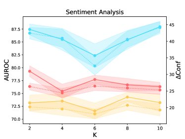
We also study the influence of the hyper-parameter K in the cross-annotation process. The results are shown in Figure 9. We observe that increasing K brings a negative or minimal effect on the calibration performance. Also, increasing K will also cause a significant increase in computational cost. Thus, the results justify our empirically chosen value K=2.

Appendix E Additional Results
Appendix F Evaluation Settings of Downstream Applications
Selective classification.
We consider two classic metrics following Kamath et al. (2020): (1) AUROCrisk: We plot the risk versus coverage curve by varying the confidence threshold, and measuring the area under this curve. In fact, this can be computed by subtracting the AUROC scores listed in Table 4 from 1. Notably, smaller AUROCrisk scores are better in selective classification, which is different from other applications; (2) Cov: The maximum possible coverage for the desired risk level. We choose Acc=95% for most tasks while choosing 85% and 60% for Semeval and HANS respectively due to PLMs’ low performance on these two datasets. We leave out the results in ANLI due to the same low-performance reason.

Adversarial defense.
In our experiments, we follow Chen et al. (2022a) to consider the security-relevant task in evaluation, and use civil comments as the evaluation dataset. We consider five attack methods, including PWWS (Ren et al., 2019), Textbugger (Li et al., 2019), BERT-Attack (Li et al., 2020), Hotflip (Ebrahimi et al., 2018), and ROCKET (Chen et al., 2022a). For each method, we generate 1,000 successful adversarial samples by attacking a well-trained T5 model.
We adopt two evaluation metrics: (1) AUROC: We measure whether the confidence in ID samples is higher than in adversarial samples; (2) Conf: The average confidence difference between ID samples and adversarial samples.
Model cascading.
In our experiments, we use a T5-small and a T5-base to constitute the model pool. Following Varshney and Baral (2022b), we measure the AUROC score in our experiments. Specifically, we vary the confidence levels, corresponding to different computational costs of the system. Then we plot the accuracy versus confidence curve and measure the area under this curve as the AUROC score.
| Amazon | Dataset | Amazon | SST-5 | SemEval | |||
|---|---|---|---|---|---|---|---|
| Method | AUROCrisk | Cov | AUROCrisk | Cov | AUROCrisk | Cov | |
| Vanilla | 14.20 | 89.82 | 20.86 | 21.37 | 28.32 | 18.40 | |
| TS | 14.27 | 90.22 | 20.86 | 23.24 | 28.11 | 18.82 | |
| LS | 18.07 | 89.28 | 23.19 | 2.81 | 29.48 | 13.35 | |
| LM-TOAST |
12.56 | 91.27 | 20.68 | 23.52 | 26.83 | 24.25 | |
| Civil | Dataset | Civil | Hate Speech | Implicit | |||
| Method | AUROCrisk | Cov | AUROCrisk | Cov | AUROCrisk | Cov | |
| Vanilla | 9.67 | 84.71 | 37.20 | 10.46 | 34.01 | 0.04 | |
| TS | 9.67 | 84.71 | 37.20 | 10.46 | 34.01 | 0.16 | |
| LS | 8.85 | 85.17 | 37.83 | 1.05 | 36.08 | 0 | |
| LM-TOAST |
7.99 | 88.03 | 34.45 | 18.83 | 34.01 | 0.16 | |
| MNLI | Dataset | MNLI | HANS | ANLI | |||
| Method | AUROCrisk | Cov | AUROCrisk | Cov | AUROCrisk | Cov | |
| Vanilla | 17.40 | 69.63 | 47.04 | 62.45 | 55.89 | - | |
| TS | 17.40 | 69.75 | 47.04 | 0 | 55.89 | - | |
| LS | 19.49 | 68.18 | 53.48 | 0 | 56.93 | - | |
| LM-TOAST |
17.26 | 71.74 | 39.40 | 79.46 | 56.03 | - | |
| Task | Dataset | Template | Verbalizer | ||||
|---|---|---|---|---|---|---|---|
| Sentiment Analysis | Amazon | It was <mask>. {”placeholder”: ”text a”} | [bad, good, neutral] | ||||
| SST-5 | It was <mask>. {”placeholder”: ”text a”} | [bad, good, neutral] | |||||
| SemEval | It was <mask>. {”placeholder”: ”text a”} | [bad, good, neutral] | |||||
| Hate Speech Detection | Civil | It was <mask>. {”placeholder”: ”text a”} | [benign, toxic] | ||||
| Hate Speech | It was <mask>. {”placeholder”: ”text a”} | [benign, toxic] | |||||
| Implicit | It was <mask>. {”placeholder”: ”text a”} | [benign, toxic] | |||||
| Natural Language Inference | MNLI |
|
[No, Yes, Maybe] | ||||
| HANS |
|
[No, Yes, Maybe] | |||||
| ANLI |
|
[No, Yes, Maybe] |
| Task | Dataset | Template | Verbalizer | ||
|---|---|---|---|---|---|
| Sentiment Analysis | Amazon |
|
[False, True] | ||
| SST-5 |
|
||||
| SemEval |
|
||||
| Hate Speech Detection | Civil |
|
|||
| Hate Speech |
|
||||
| Implicit |
|
||||
| Natural Language Inference | MNLI |
|
|||
| HANS |
|
||||
| ANLI |
|