Manifold attack
Abstract
Machine Learning in general and Deep Learning in particular has gained much interest in the recent decade and has shown significant performance improvements for many Computer Vision or Natural Language Processing tasks. In this paper, we introduce manifold attack, a combination of manifold learning and adversarial learning, which aims at improving neural network models regularization. We show that applying manifold attack provides a significant improvement for robustness to adversarial examples and it even enhances slightly the accuracy rate. Several implementations of our work can be found in https://github.com/ktran1/Manifold-attack.
Index terms Deep learning, Robustness, Manifold learning, Adversarial learning, Geometric structure, Semi-Supervised learning.
1 Introduction
Deep Learning (DL) [1] has been first introduced by Alexey Ivakhnenko (1967), then its derivative Convolutional Neural Networks [2] (1980) has been introduced by Fukushima. Over the years, it was improved and refined in by Yann LeCun [3] (1998). Up to now, deep neural networks have yield groundbreaking performances at various classification tasks [4, 5, 6, 7, 8]. However, training deep neural networks involves different regularization techniques, which are primordial in general for two goals: generalization and adversarial robustness. On the one hand, regularization for generalization aims at improving the accuracy rate on the data that have not been used for training. In particular, this regularization is critical when the number of training samples is relatively small compared to the complexity of neural network model. On the other hand, regularization for adversarial robustness aims at improving the accuracy rate with respect to adversarial samples.
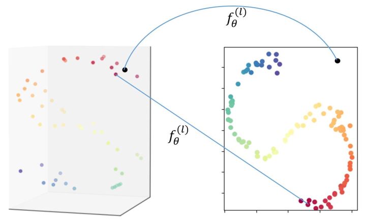
In the last few years, a lot of research works in machine learning focus on getting high performance models in terms of adversarial robustness without losing in generalization. Our work focuses on the preservation of geometric structure (PGS) between the original representation of data and a latent representation produced by a neural network model (NNM). PGS is part of manifold learning techniques: we assume that the data of interest lies on a low dimensional piecewise smooth manifold with respect to which we want to compute original samples embeddings. In neural network models (NNMs), the output of the hidden layers are considered to be candidate low dimensional embeddings. For classification tasks, combining PGS as a regularization loss with supervised loss was shown to improve generalization ability by Weston et al. in 2008 [9]. The concept of adversarial samples was later introduced by Goodfellow et al. [10] in 2014, as NNMs architecture became deeper and hence more complex. Adversarial robustness in NNMs is strictly related to the PGS, since PGS for NNMs precisely aims at ensuring that the NNM gives similar outputs for close inputs. Figure 1 shows an illustration of PGS including a failure example. The black point can be considered an adversarial example for the dimension reduction model.
The novelty of this paper is to reinforce PGS by introducing synthetic samples as supplementary data. We make use of adversarial learning methodology to compute relevant synthetic samples. Then, these synthetic samples are added to the original real samples for training the model which is expected to improve adversarial robustness.
Contributions :
-
•
We present the concept of manifold attack to reinforce PGS task.
-
•
We show empirically that by applying manifold attack for a classification task, NNMs get better in both adversarial robustness and generalization.
The outline of the paper is as follows. In section 2, we present related works that aim to increase adversarial robustness of NNMs. In section 3, we revisit some classical PGS methods. In section 4, we present manifold attack. The numerical experiments are presented and discussed in section 5. Our conclusions and perspectives are presented in section 6.
2 Related works
In this section, we present several strategies to reinforce adversarial robustness, sorting them into two categories.
The first category is related to off-manifold adversarial examples i.e. adversarial examples that lies off the data manifold. In a supervised setting, these adversarial examples are used for training model as additional data[10]. In a semi-supervised setting, these adversarial examples are used to enhance the consistency between representations [11]. In plain words, a sample and its corresponding adversarial example must have a similar representation at the output of model. However, some works [12, 13] state that adversarial robustness with respect to off-manifold adversarial examples is in conflict with generalization. In other words, improving adversarial robustness is detrimental to generalization and vice versa.
In the second category, the adversarial robustness is reinforced with respect to on-manifold adversarial examples [14, 15, 16]. In all these works, a generative model such as VAE[17], GAN[18] or VAE-GAN [19] is firstly learnt, so that one can generate a sample on the data manifold from parameters in a latent space. These works differ in the technique used to create adversarial noise in the latent space to produce on-manifold adversarial examples. Finally, these on-manifold adversarial examples are used as additional data for training model. Interestingly, by using on-manifold adversarial examples, [15] states that adversarial robustness and generalization can be jointly enhanced. We note that a hybrid approach has been proposed in [20] where both off-manifold and on-manifold adversarial examples are used as supplement data for training model.
Our method falls into the second category since we want to enhance both the adversarial robustness and the generalization in both supervised and semi-supervised settings. However the adversarial examples are generated using a different paradigm.
3 Preservation of geometric structure
In most cases, a PGS process has two stages: extracting properties of original representation then computing an embedding which preserves these properties into a low dimensional space. Given a data set , and its embeddings set , where is the embedded representation of , we note:
| (1) |
the embedding loss, where is the complement of in . The objective function of PGS is then defined as:
| (2) |
We present some popular embedding losses hereafter:
- Multi-Dimensional scaling (MDS) [21]:
| (3) |
where and are measures of dissimilarity. By default, they are both Euclidean distances. This method aims at preserving pairwise distances from the original representation in the embedding space.
- Laplacian eigenmaps (LE) [22]:
| (4) |
where is a measure of similarity measure (for instance ) and is a measure of dissimilarity (for instance ). This method learns manifold structure by emphasizing the preservation of local distances. In order to further reduce effect of large distances, in some papers, is set directly to zero if is not in the nearest neighbors of or vice versa if is not in the nearest neighbors of . Alternatively, one can set if . Let be the matrix defined as hence is a symmetric matrix if is symmetric. We can represent the objective function of Laplacian eigenmaps method using the matrices:
| (5) |
where , ( being a diagonal matrix). a graph Laplacian matrix because it is symmetric, the sum of each row equals to 1 and its elements are negatives except for the diagonal elements.
- Locally Linear Embedding (LLE) [23]:
| (6) |
where are determined by solving the following problem:
| (7) |
where knn() denotes a set containing indices of the nearest neighbors samples (in Euclidean distance) of the sample . Assuming that the observed data is sampled from a smooth manifold and provided that the sampling is dense enough, one can assume that the sample lies locally on linear patches. Thus, LLE first computes the barycentric coordinate for each sample w.r.t. its nearest neighbors. These barycentric coordinates characterize the local geometry of the underlying manifold. Then, LLE computes a low dimensional representation (embedded) which is compatible with these local barycentric coordinates. Introducing a matrix representation form for as: then can be rewritten as , where . Thus, the loss can be interpreted as Laplacian eigenmaps loss, based on an implicit metric for measuring distance between two samples.
- Contrastive loss :
where is a discrete similarity metric which is equal to 1 if is in the neighborhood of and 0 otherwise. is a measure of dissimilarity.
- Stochastic Neighbor Embedding (SNE) [24]:
where and , and are both similarity metric. The objective of this method is to preserve the similarity between two distributions of pairwise distances, one in original representation and the other in embedded representation, by Kullback–Leibler (KL) divergence.
Traditionally, PGS finds its applications in dimensionality reduction or data visualization, which refers to the techniques used to help the analyst see the underlying structure of data and explore it. For instance, [25] proposes a variant of SNE, which has been used in a wide range of fields. Classical nonlinear PGS methods do not require a mapping model, which is a function with trainable parameters that maps a sample x to its embedded representation as . is directly used as the optimization variable.
Finally, it is worth noting that for several PGS methods such as LE and LLE, some supplement constraints are required to avoid a trivial solution (for instance with all embedded points are collapsed into only one point). Usually, mean and co-variance constrains are applied:
| (8) |
4 Manifold attack
We introduce a new strategy called “manifold attack” to reinforce PGS methods with mapping model, by combining with adversarial learning. In the following denotes a differentiable function that maps a sample to its embedded representation .
4.1 Individual attack point versus data points
We define a virtual point is a synthetic sample generated in such a way to be likely on the observed samples underlying manifold. An anchor point is a sample used for generating a virtual point. An attack point is a virtual point that maximises locally a chosen measure of model distortion. For example, attack point can be a sample perturbed with an adversarial noise.
We use the same notation as in section 3. Given a dataset and the corresponding embedded set , denotes the embedding loss, being the complement of in . We consider the objective function of PGS defined as . Let’s consider anchor points , a virtual point is defined as:
| (9) |
The anchor points define a region or feasible zone, in which a virtual point must be located and is the coordinate of . Anchor points are sampled from the dataset with different strategies, which are defined according to predefined rules (see section 4.4 for several examples). Figure 2 shows an example of anchor points setting and relations between points. For the embedding of observed sample , , the embedding loss is defined as:
| (10) |
Similarly, for the embedding of virtual point , , the embedding loss is defined as:
| (11) |
The algorithm 1 describes the computation of an attack point. It consists in finding the local coordinates that maximizes the embedding loss for the current state of model . Hence, is estimated though a projected gradient ascent.
In order to guarantee the constrains in equation (9), we use the projector defined by the problem:
| (12) |
This convex problem with constraints can be solved quickly by a simple sequential projection that alternates between sum constraint and positive constraint (algorithm 2). The demonstration can be inspired by Lagrange multiplier method. A simple demonstration can be found in Appendix.
By default, each set of anchor points has one attack point. However, we can generate more than one attack point for the same set of anchor points by using different initializations of , so as to find different local maxima. The double embedding loss, on the observed samples and on the attack points, is expected to enforce the the model smoothness over the underlying manifold, including in low samples density areas. The general optimization scheme goes as follows: we optimize alternately between attack stages and model update stages until convergence. In attack stage, we optimize the attack points through while fixing the model and in the model update stage, we optimize the model while fixing attack points.
4.2 Attack points as data augmentation
In algorithm 1, an attack points only interacts with observed samples. In the general manifold attack (algorithm 3), attack points and observed samples are undifferentiated in the model update stage. This way, hence generating attack points can be considered a data augmentation technique. We denote as a set that contains all embedded points (both attack points and observed samples). is a random subset of , used batch for batch optimization. In each step, only attack points from the current batch are used to distort the manifold by maximizing the batch loss .
Algorithm 4 represents the update step for multiple attack points. We assumed that the embedding loss is smooth with respect to and used a gradient-based algorithm to estimate the latter. Nevertheless, in PGS, there are several methods whose embedding loss is not even continuous. For example, in LLE (6), the embedding loss takes into account the nearest neighbors of a point, which might change throughout the estimation of an attack point, producing a discontinuity. To circumvent this problem, we use several strategies to avoid singularities:
-
-
By reducing the gradient step which limits the virtual point displacement.
-
-
By taking a small number of attack points in each subset or by using randomly a part of attack points to perform the attack while fixing other attack points, in an attack stage.
-
-
By updating only if embedding loss increases.
Besides, some metrics might be approximated by smooth functionals. For instance, in the contrastive loss (3), we can replace the metric which outputs only 0 or 1, with to make embedding loss continuous.
4.3 Pairwise preservation of geometric structure
For some PGS methods as MDS or LE, the embedding loss can be decomposed into the sum of elementary pairwise loss :
| (13) |
Then the batch loss (in algorithm 3) can be modified into:
| (14) |
Following this change, can be decomposed into three parts:
where and are respectively set that contains all embedded data points (or observed samples) and all embedded virtual points of .
In some PGS losses which can be decomposed into the sum of elementary pairwise loss, we can balance the effect of the virtual points with respect to the observed samples, not only by tuning the ratio between the number of virtual points and the number of observed samples in , but also by weighting each of three parts above which corresponds to the settings observed-observed, observed-virtual and virtual-virtual.
4.4 Settings of anchor points and initialization of virtual points
In this section, we provide two settings (or rules) for computing anchor points with the corresponding initializations. These settings need to be chosen carefully to guarantee that virtual points are on the sample underlying manifold.
Neighbor anchors: The first anchor point is taken randomly from , then the next anchor points are taken as nearest neighbor points of in (Euclidean metric by default). Here, we assume that the convex hull of a sample and its neighbors is likely comprised in the samples manifold. The number of anchors needs to be small compared to the number of data points . The initialization for virtual points can be set by taking then normalize to have .
Random anchors: The second setting is inspired by Mix-up method [26]. anchors are taken randomly from and we take . If , the Dirichlet distribution returns where , . In particular, there is a coefficient much greater than other ones with a strong probability, which implies that virtual points are more probably in the neighborhood of a data sample. Since the manifold attack tries to find only local maximum by gradient-based method, if and are both small, we expect that attack points in the attack stage do not move too far from their initiated position, remaining on the manifold of data. Note that, in the case , the Dirichlet distribution become the Uniform distribution.
To ensure that the coefficient is always much greater than other ones, we apply one more constraint: , and by taking close to 1. The constraints in (9) become:
| (15) |
Then the projection in algorithm 2 needs to be slightly modified to incorporate this new constraint. We define the projection as follow:
| (16) |
5 Applications of manifold attack
We present several applications of manifold attack for NNMs that use PGS task. Firstly, we show advantages of manifold attack for a PGS task when only few training samples are available. Secondly, we show that applying manifold attack in moderation improves both generalization and adversarial robustness.
5.1 Preservation of geometric structure with few training samples
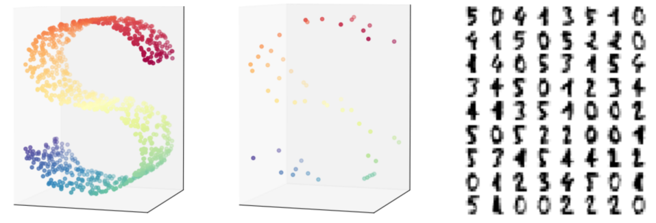
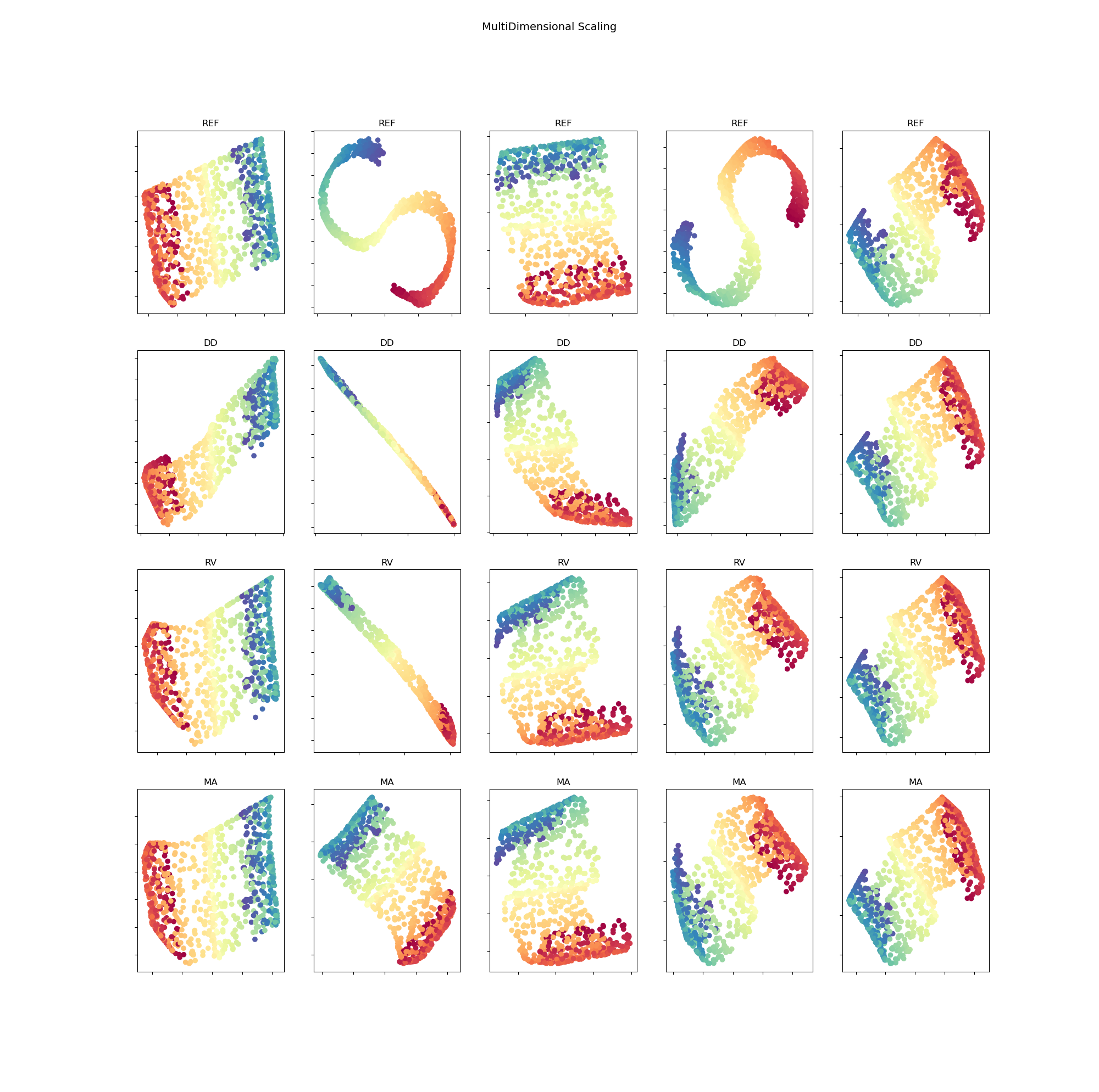
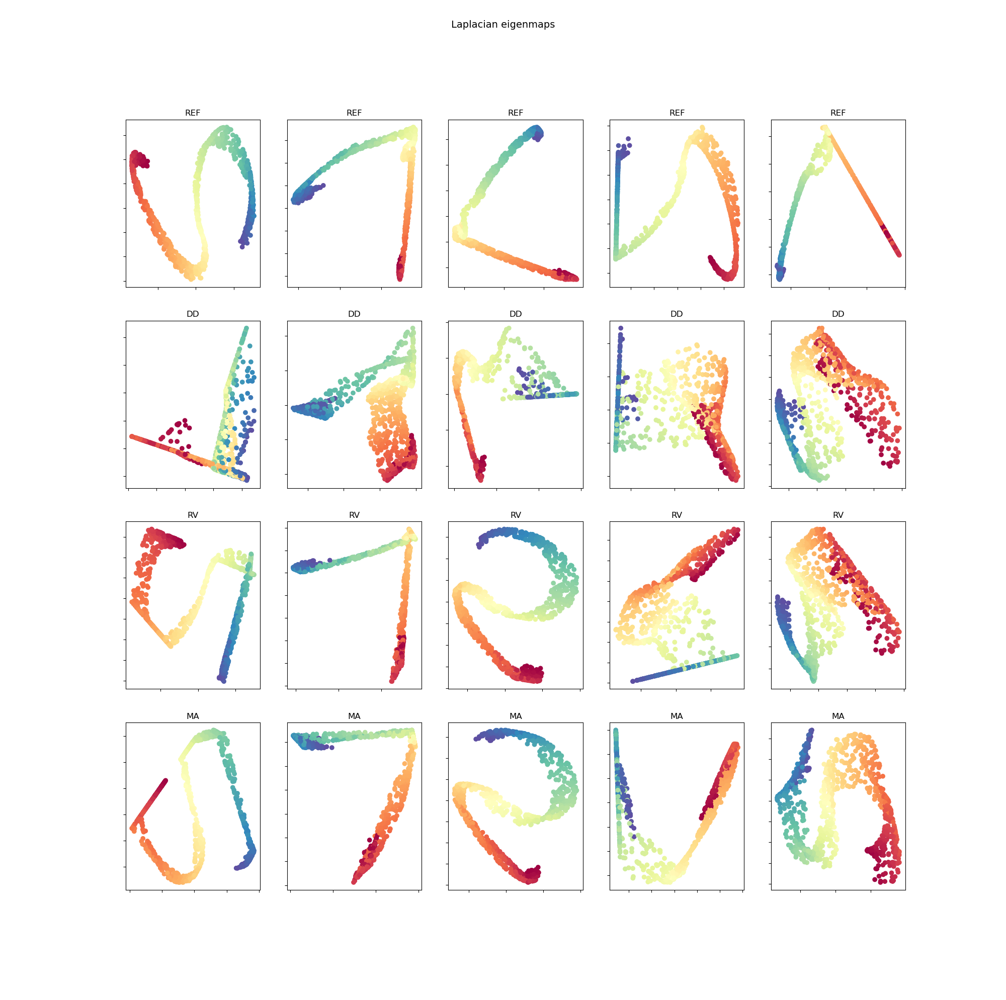
For this experiment, we use the S curve data and Digit data. The S curve data contains 3-dimensional samples, as shown in figure 3. The Digit data contains images, of size of a digit. We want to compute 2-dimensional embeddings for these data. Each data is separated into two sets: samples are randomly taken for training set and the remaining samples are used for testing. denotes a training sample and denotes a testing sample. We perform four training modes as described in table 1 with a neural network model . The evaluation loss, after optimizing model , is defined as:
| (17) |
| Mode | Description of objective function |
| 1. REF | PGS that takes into account both training and testing samples: The result of this training mode is considered as “reference” in order to compare to other training modes. |
| 2. DD | PGS that takes only training (observed) data samples: |
| 3. RV | Using virtual points as supplement data, virtual points are only randomly initialized and without attack stage (by setting in algorithm 4): where . |
| 4. MA | Using manifold attack, the same objective function as the previous case, except (virtual points become attack points). |
The anchoring rule, embedding loss and the model are precised in the following.
Anchoring rule. Two settings are considered:
-
-
Neighbor anchors (NA): A set of anchor points is composed by a sample with its 4 nearest neighbors. In this case, we have sets of anchor points and anchor points in each set. The coefficient is initialized by uniform distribution.
-
-
Random anchors (RA): We take randomly 2 points among training points to create a set of anchor points. In this case, we have sets of anchor points and anchor points in each set. The coefficient is initialized by the Dirichlet distribution with .
The embedding loss. We employ the embedding loss MDS and LE as described in section 3, with the default metrics. For similarity metric in LE method, we take for S curve data and for Digit data.
The model. A simple structure of CNN is used. Here are the detailed architectures for each CNN as the dimension of the inputs are different for the two datasets:
-
-
S curve data: Conv1d[] ReLu Conv1d[] ReLu Flatten Fc[].
-
-
Digit data: Conv2d[] ReLu Conv2d[] ReLu Flatten Fc[].
For LE method, two additional constraints are imposed to avoid trivial embeddings:
| (18) |
where is the number of output dimensions, . To adapt these constraints, we add a normalization layer at the end of model : , where is performed by Cholesky decomposition.
To simulate the case of few training samples, we fix for MDS method and for LE method. The balance between virtual points and samples is controlled by the couple (number of virtual points in , number of observed samples in ). We set for MDS method and for LE method. The gradient step is selected from and the number of iterations is fixed at .
The initialization of model is impactful, especially since there are few training data. Five different initialization of model for each method are performed. The mean and the standard deviation of the evaluation loss are represented in table 2. Firstly, we see that using random virtual (RV) points as additional data points gives a better loss than using only data points. Secondly, using manifold attack (MA) further improves the results which shows the benefit of the proposed approach to regularize the model.
For the S curve data, initialization by Neighbors anchors (NA) gives a better result compared to initialization by Random anchors (RA). However, for the Digit data, initialization by Random anchors gives a better result. This is due to the fact that in the S curve data, Neighbor Anchors covers better the manifold of data than Random Anchor. On the other hand, in Digit data, Neighbor Anchors (by using Euclidean metric to determine nearest neighbors) can generate, with greater probability, a virtual point that is not in the manifold of data. This leads to a greater evaluation loss compared to Random Anchor.
| S curve data | Digit data | |||
| Mode / Method | MDS | LE | MDS | LE |
| REF | ||||
| DD | ||||
| RV (NA) | ||||
| MA (NA) | ||||
| RV (RA) | ||||
| MA (RA) | ||||
The five embedded representations, respectively with five different initialization of , for testing samples in S curve data are found in figure 4 for MDS method and in figure 5 for LE method.
5.2 Robustness to adversarial examples
In this subsection, we combine manifold attack with supervised learning to assess the adversarial robustness of model. Let start with a general objective function which is created by a supervised loss and a PGS loss :
| (19) |
where means a sample and its corresponding label. is a dissimilarity metric, like for instance the Cross Entropy. is a PGS loss that includes eventually all observed samples and virtual points . Note that the coordinates of all virtual points are constrained by (9).
In the following, we construct by a particular PGS loss, called Mix-up manifold learning loss [27, 28, 26] :
| (20) |
In this configuration, the virtual point , where and are two anchor points. The distribution Beta is just a particular case of the Dirichlet distribution where the number of anchor points (in section 4.4). In case of supervised learning, we perform PGS between the original samples representation and the final NNM output (which can be considered as a latent representation). Thus, we implement a slightly modified version of equation (20):
| (21) |
Then, we replace this explicit PGS loss in equation (5.2) and take :
| (22) | ||||
| (23) | ||||
| where: | (24) | |||
| (25) |
We call problem (22) adversarial Mix-up because this problem is developed from Mix-up[26], by adding an adversarial learning for . In practice, to optimize the problem (22), we perform an attack stage (algorithm 4) to find that gives the greater PGS loss, before performing model update stage for . We repeat alternatively these two stages until convergence. Note that, we can take , so that we only need to deal with one variable to maximize PGS loss. The projection (12) for is now just the clamping function, to make sure that is between 0 and 1.
We compare four supervised training methods: ERM (Empirical Risk Minimization, which is thus classical supervised learning with Cross Entropy loss), Mix-up, Adversarial Mix-up and Cut-Mix [29] on ImageNet dataset with the model ResNet-50 [6], which has about 25.8M trainable parameters. We use ImageNet dataset. We retrieve 948 classes consisting in 400 labelled training samples and 50 testing samples to evaluate the models.
| Method / Data evaluation | Testing set | Adversarial examples | ||
| Top-1 | Top-5 | Top-1 | Top-5 | |
| ERM | 33.84 | 12.46 | 81.69 | 59.14 |
| Mix-up [26] | 32.13 | 11.35 | 75.57 | 49.41 |
| Mix-up Adversarial (1) () | 32.57 | 10.98 | 63.62 | 36.15 |
| Adversarial Mix-up (2) () | 31.82 | 11.15 | 70.82 | 43.96 |
| Cut-Mix [29] | 30.94 | 10.41 | 81.24 | 58.72 |
We evaluate the error rate for testing set at the end of each epoch and report the best best error rate (top-1 and top-5) in table 3. We create adversarial examples using Fast Gradient Sign Method (FGSM) [10], on another trained ERM model, with . In Adversarial Mix-up, is fixed at 1. The attack stage is parametrized by the gradient step , which is set up following two configurations, (1) is reduced linearly from 0.1 to 0.01 and (2) is reduced linearly from 0.01 to 0.001. Following original articles, is set at 0.2 for Mix-Up and Adversarial Mix-up and for Cut-Mix. More details for hyper-parameters can be found in Appendix.
Firstly, Mix-up [26] is a combination between supervised learning task and PGS task loss and it gives a better error rates for both testing set and adversarial examples compared to ERM, which is a standard supervised learning task.
Secondly, in Adversarial Mix-up (1) and (2), a trade-off has to be found between error rate for testing set and error rate for adversarial examples. For strong values of (1), the error rate for testing sample can be about 0.5% worse than Mix-up (without using attack stage), but it gains about 13% for the robustness against adversarial examples. On the other hand, if takes moderate values as in (2), error rates for both testing sample and adversarial examples are smaller than those of Mix-Up, but it gains only about 5% for the robustness against adversarial examples. These two observations show the effect of manifold attack, which is an improved PGS procedure. We conclude that manifold attack not only improves generalization but also significantly improves adversarial robustness of the model.
Finally, Adversarial Mix-up Adversarial (2) provides a slightly worse error rate than Cut-Mix (about 1 % in the case of testing sample), but it gains about 10% in the case of adversarial examples.
It is worth noting that in attack stage, the model needs to be differentiable. Thus, in the case of using NNMs with Dropout layer for example , the active connections need to be fixed during an attack stage.
5.3 Semi-supervised manifold attack
In this subsection, manifold attack is applied to reinforce semi-supervised neural network models that use PGS as regularization. The problem (5.2) is extended to include unlabelled samples. We assume that the training set contains samples , the first samples are labelled and the remaining samples are unlabelled. Hence, the objective function for a semi-supervised manifold attack method:
| (26) |
where refers to other possible unsupervised losses such as pseudo-label, self-supervised learning, etc.
In the following, we explicit the terms of the problem (26). We build upon MixMatch [30], a semi-supervised learning method in the current state-of-the-art. MixMatch use Mix-up manifold learning loss for PGS. Secondly, we add an adversarial learning for in MixMatch. Hence we refer to the resulting instance of 26 as Adversarial MixMatch. Note that, in MixMatch is slightly different from Mix-up as:
| (27) |
Then the projection for is now the clamping function between 0.5 and 1. When two separated variables and are defined, we can use the projector (16) defined in subsection 4.4. We use the Pytorch implementation for MixMatch by Yui [31] (with all hyper-parameters by default), then we introduce attack stages, with the number of iterations . In each experiment, for both CIFAR-10 and SVHN dataset, we divide the training set into three parts: labelled set, unlabelled set and validation set. The number of validation samples is fixed at 5000. The number of labelled samples is 250, and the remaining samples are part of the unlabelled set. We repeat the experiment four times, with different samplings of labelled samples, unlabelled samples, validation samples and different initialization of model Wide ResNet-28 [32] which has about 1.47M trainable parameters. More details for hyper-parameters can be found in Appendix.
| Data | Method / Test | 1 | 2 | 3 | 4 | Mean |
| CIFAR-10 | MixMatch | 10.62 | 12.72 | 12.02 | 15.26 | |
| CIFAR-10 | MixMatch Adersarial | 8.84 | 10.46 | 10.09 | 12.89 | |
| SVHN | MixMatch | 6.0925 | 6.73 | 7.802 | 7.37 | |
| SVHN | MixMatch Adersarial | 5.07 | 5.93 | 5.42 | 5.47 |
The error rate on testing set, which corresponds to the best validation error rate, is reported in table 4, for both MixMatch and MixMatch Adersarial. We see that MixMatch Adersarial improves the performance of MixMatch, about less on error rate. There is a considerable difference between the error rate of MixMatch reproduced by our experiments and the one reported from the official paper, which might come from the sampling, the initialization of model, the library used (Pytorch vs TensorFlow) and the computation of the error rate (error rate associated to best validation error vs the median error rate of the last 20 checkpoints).
| Method / Data | CIFAR-10 | SVHN |
| Pi Model ⋄ [33] | ||
| Pseudo Label ⋄ [34] | ||
| VAT ⋄ [11] | ||
| SESEMI SSL [35] | ||
| Mean Teacher ⋄ [36] | ||
| Dual Student [37] | ||
| MixMatch ⋄ [30] | ||
| MixMatch * [30] | ||
| MixMatch Adersarial * | ||
| Real Mix [38] | ||
| EnAET [39] | ||
| ReMixMatch [40] | ||
| Fix Match [41] |
Table 5 shows error rates among semi-supervised methods based on NNMs, for both CIFAR-10 and SVHN dataset with only 250 labelled samples. We refer also readers to the site PapersWithCode that provides the lasted record for each dataset: CIFAR-10111CIFAR-10 https://paperswithcode.com/sota/semi-supervised-image-classification-on-cifar-6 and SVHN 222SVHN https://paperswithcode.com/sota/semi-supervised-image-classification-on-svhn-1.
6 Conclusion
| Adversarial Example | Manifold Attack | |||||
|
||||||
| Feasible zone | Locality of each sample | Convex hull | ||||
| Variable | Noise that has the same size as samples | has the size which equals to the number of anchor points | ||||
| PGS task | Points in the locality of a sample must have a similar embedded representation | Available for almost PGS tasks | ||||
We introduced manifold attack as an improved PGS procedure. Firstly, it is more general than adversarial examples (see for a comparison in table 6). Secondly, we confirm empirically a statement from [26]: by using Mix-up as PGS combined with supervised loss, we enhance generalization and improve significantly adversarial robustness. Thirdly, we show that applying manifold attack on Mix-up enhances further generalization and adversarial robustness. There is a trade-off to be found between generalization and adversarial robustness. However, in our experiments, in the ’worst case’, we only lose about 1% in generalization for a gain of about 13% in adversarial robustness.
To further improve our method, several directions could be investigated:
-
•
Optimization of the layers between those the PGS needs to be applied. Indeed, we could also implement PGS between one latent representation and another one in NNMs as in [28].
-
•
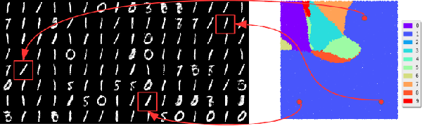
Mode collapse is a popular problem while training GAN models. GAN with samples that are well balanced among classes, generated samples by the generator are biased on only a few classes (as showed in figure 6). This is because the latent representation is not well regularized. We expect to overcome the problem Mode collapse by introducing manifold attack from the latent representation back to the original representation as show in figure 7 and by optimizing problem 28, where is a PGS task as showed in section 3.
| (28) |
Acknowledgement
This research is supported by the European Community through the grant DEDALE (contract no. 665044) and the Cross-Disciplinary Program on Numerical Simulation of CEA, the French Alternative Energies and Atomic Energy Commission.
References
- [1] Yann Lecun, Yoshua Bengio, and Geoffrey Hinton. Deep learning. Nature Cell Biology, 521(7553):436–444, may 2015.
- [2] K Fukushima. Neocognitron: a self organizing neural network model for a mechanism of pattern recognition unaffected by shift in position. Biological cybernetics, 36(4):193—202, 1980.
- [3] Y. Lecun, L. Bottou, Y. Bengio, and P. Haffner. Gradient-based learning applied to document recognition. Proceedings of the IEEE, 86(11):2278–2324, 1998.
- [4] Alex Krizhevsky, Ilya Sutskever, and Geoffrey E Hinton. Imagenet classification with deep convolutional neural networks. In F. Pereira, C. J. C. Burges, L. Bottou, and K. Q. Weinberger, editors, Advances in Neural Information Processing Systems 25, pages 1097–1105. Curran Associates, Inc., 2012.
- [5] Karen Simonyan and Andrew Zisserman. Very deep convolutional networks for large-scale image recognition, 2014.
- [6] Kaiming He, Xiangyu Zhang, Shaoqing Ren, and Jian Sun. Deep residual learning for image recognition. CoRR, abs/1512.03385, 2015.
- [7] Christian Szegedy, Wei Liu, Yangqing Jia, Pierre Sermanet, Scott E. Reed, Dragomir Anguelov, Dumitru Erhan, Vincent Vanhoucke, and Andrew Rabinovich. Going deeper with convolutions. CoRR, abs/1409.4842, 2014.
- [8] G. Hinton, L. Deng, D. Yu, G. E. Dahl, A. Mohamed, N. Jaitly, A. Senior, V. Vanhoucke, P. Nguyen, T. N. Sainath, and B. Kingsbury. Deep neural networks for acoustic modeling in speech recognition: The shared views of four research groups. IEEE Signal Processing Magazine, 29(6):82–97, 2012.
- [9] Jason Weston and Frédéric Ratle. Deep learning via semi-supervised embedding. In International Conference on Machine Learning, 2008.
- [10] Ian J. Goodfellow, Jonathon Shlens, and Christian Szegedy. Explaining and harnessing adversarial examples, 2014.
- [11] Takeru Miyato, Shin ichi Maeda, Masanori Koyama, and Shin Ishii. Virtual adversarial training: A regularization method for supervised and semi-supervised learning, 2017.
- [12] Dong Su, Huan Zhang, Hongge Chen, Jinfeng Yi, Pin-Yu Chen, and Yupeng Gao. Is robustness the cost of accuracy? – a comprehensive study on the robustness of 18 deep image classification models, 2019.
- [13] Dimitris Tsipras, Shibani Santurkar, Logan Engstrom, Alexander Turner, and Aleksander Madry. Robustness may be at odds with accuracy, 2019.
- [14] Yang Song, Rui Shu, Nate Kushman, and Stefano Ermon. Constructing unrestricted adversarial examples with generative models, 2018.
- [15] David Stutz, Matthias Hein, and Bernt Schiele. Disentangling adversarial robustness and generalization, 2019.
- [16] Ousmane Amadou Dia, Elnaz Barshan, and Reza Babanezhad. Semantics preserving adversarial learning, 2019.
- [17] Diederik P Kingma and Max Welling. Auto-encoding variational bayes, 2013.
- [18] Ian J. Goodfellow, Jean Pouget-Abadie, Mehdi Mirza, Bing Xu, David Warde-Farley, Sherjil Ozair, Aaron Courville, and Yoshua Bengio. Generative adversarial nets. In Proceedings of the 27th International Conference on Neural Information Processing Systems - Volume 2, NIPS’14, page 2672–2680, Cambridge, MA, USA, 2014. MIT Press.
- [19] Anders Boesen Lindbo Larsen, Søren Kaae Sønderby, Hugo Larochelle, and Ole Winther. Autoencoding beyond pixels using a learned similarity metric, 2016.
- [20] Wei-An Lin, Chun Pong Lau, Alexander Levine, Rama Chellappa, and Soheil Feizi. Dual manifold adversarial robustness: Defense against lp and non-lp adversarial attacks, 2020.
- [21] J.B. Kruskal and M. Wish. Multidimensional Scaling. Sage Publications, 1978.
- [22] Mikhail Belkin and Partha Niyogi. Laplacian eigenmaps for dimensionality reduction and data representation. Neural Computation, 15:1373–1396, 2003.
- [23] Sam T. Roweis and Lawrence K. Saul. Nonlinear dimensionality reduction by locally linear embedding. SCIENCE, 290:2323–2326, 2000.
- [24] Geoffrey Hinton and Sam Roweis. Stochastic neighbor embedding. Advances in neural information processing systems, 15:833–840, 2003.
- [25] L.J.P. van der Maaten and G.E. Hinton. Visualizing high-dimensional data using t-sne. Journal of Machine Learning Research, 9(nov):2579–2605, 2008. Pagination: 27.
- [26] Hongyi Zhang, Moustapha Cissé, Yann N. Dauphin, and David Lopez-Paz. mixup: Beyond empirical risk minimization. CoRR, abs/1710.09412, 2017.
- [27] Vikas Verma, Alex Lamb, Juho Kannala, Yoshua Bengio, and David Lopez-Paz. Interpolation consistency training for semi-supervised learning, 2019.
- [28] Vikas Verma, Alex Lamb, Christopher Beckham, Amir Najafi, Ioannis Mitliagkas, Aaron Courville, David Lopez-Paz, and Yoshua Bengio. Manifold mixup: Better representations by interpolating hidden states, 2019.
- [29] Sangdoo, Dongyoon Han, Seong Joon Oh, Sanghyuk Chun, Junsuk Choe, and Youngjoon Yoo. Cutmix: Regularization strategy to train strong classifiers with localizable features. CoRR, abs/1905.04899, 2019.
- [30] David Berthelot, Nicholas Carlini, Ian Goodfellow, Nicolas Papernot, Avital Oliver, and Colin Raffel. Mixmatch: A holistic approach to semi-supervised learning, 2019.
- [31] Yui. Pytorch Implementation for Mix Match, 2019. imikushana@gmail.com.
- [32] Sergey Zagoruyko and Nikos Komodakis. Wide residual networks, 2016.
- [33] Samuli Laine and Timo Aila. Temporal ensembling for semi-supervised learning. CoRR, abs/1610.02242, 2016.
- [34] Dong hyun Lee. Pseudo-label: The simple and efficient semi-supervised learning method for deep neural networks, 2013.
- [35] Phi Vu Tran. Exploring self-supervised regularization for supervised and semi-supervised learning, 2019.
- [36] Antti Tarvainen and Harri Valpola. Weight-averaged consistency targets improve semi-supervised deep learning results. CoRR, abs/1703.01780, 2017.
- [37] Zhanghan Ke, Daoye Wang, Qiong Yan, Jimmy Ren, and Rynson W. H. Lau. Dual student: Breaking the limits of the teacher in semi-supervised learning, 2019.
- [38] Varun Nair, Javier Fuentes Alonso, and Tony Beltramelli. Realmix: Towards realistic semi-supervised deep learning algorithms, 2019.
- [39] Xiao Wang, Daisuke Kihara, Jiebo Luo, and Guo-Jun Qi. Enaet: Self-trained ensemble autoencoding transformations for semi-supervised learning, 2019.
- [40] David Berthelot, Nicholas Carlini, Ekin D. Cubuk, Alex Kurakin, Kihyuk Sohn, Han Zhang, and Colin Raffel. Remixmatch: Semi-supervised learning with distribution alignment and augmentation anchoring, 2019.
- [41] Kihyuk Sohn, David Berthelot, Chun-Liang Li, Zizhao Zhang, Nicholas Carlini, Ekin D. Cubuk, Alex Kurakin, Han Zhang, and Colin Raffel. Fixmatch: Simplifying semi-supervised learning with consistency and confidence, 2020.
- [42] Ngoc-Trung Tran, Tuan-Anh Bui, and Ngai-Man Cheung. Dist-gan: An improved gan using distance constraints, 2018.
Appendix
Projection for sum and positive
Proof, by using Lagrange multiplier, problem (12) becomes:
We solve the following system of equations:
In the case that . From the second equation, we infer that (because if and as in inequality 5, then , in contradiction to inequality 6). From , we infer that with equation 4.
In the case that . From the second equation, first if then since as in equation 5. With inequality 6, we infer . Second, if , then we infer that with equation 4.
Let’s and . We find exactly the same problem as before, but with only active index in the set .
Then we repeat until the constraint satisfaction for . For a proof of convergence, as has exactly elements , then each time we project to get a new active set , we reduce the number of active elements . As the number of active elements is something positive and it decreases, so it converges. Here is an implementation for multiple () in pytorch.
Manifold attack for embedded representation
Architecture of model (Pytorch style) :
-
-
S curve data : Conv1d[] ReLu Conv1d[] ReLu Flatten Fc[].
-
-
Digit data : Conv2d[] ReLu Conv2d[] ReLu Flatten Fc[].
Optimizer : Stochastic gradient descent, with learning rate and momentum = 0.9. Learning rate is reduce by after each 10 epochs. The number of epochs is 40.
Robustness to adversarial examples
Hyper-parameters : optimizer = Stochastic gradient descent, number of epochs = 300, learning rate = 0.1, momentum = 0.9, learning rate is reduce by after each 75 epochs, batch size = 200, weight decay = 0.0001.
Semi-supervised manifold attack
Hyper-parameters : optimizer = Adam, number of epochs = 1024, learning rate = 0.002, , batch size labelled = batch size unlabelled = 64, T = 0.5 (in sharpening), (linearly ramp up from 0), EMA = 0.999 , error validation after 1024 batchs.
To reproduce an experiment, we define function seed_ as:
The four experiment 1,2,3,4 in table 4 are launched with respectively seed_(0), seed_(1), seed_(2), seed_(3).
In Mix-up Adversarial, is fixed at 1. In dataset CIFAR-10, starts at 0.1 and decreases linearly to 0.01 after 1024 epochs. In dataset SVHN, starts at 0.1 and decreases linearly to 0.01 after 1024 epochs for seed_(0) and seed_(3); starts at 0.1 and decreases linearly to 0.001 after 1024 epochs for seed_(2); starts at 0.01 and decreases linearly to 0.001 after 1024 epochs for seed_(1)