††thanks: On academic leave from Department of Physics and Astronomy, University of Pittsburgh, Pittsburgh PA 15260, USA
Manipulating Goldstone modes via the superradiant light in a bosonic lattice gas inside a cavity
Huan Wang
MOE Key Laboratory for Nonequilibrium Synthesis and Modulation of Condensed Matter,Shaanxi Province Key Laboratory of Quantum Information and Quantum Optoelectronic Devices, School of Physics, Xi’an Jiaotong University, Xi’an 710049, China
Shuai Li
MOE Key Laboratory for Nonequilibrium Synthesis and Modulation of Condensed Matter,Shaanxi Province Key Laboratory of Quantum Information and Quantum Optoelectronic Devices, School of Physics, Xi’an Jiaotong University, Xi’an 710049, China
Maksims Arzamasovs
MOE Key Laboratory for Nonequilibrium Synthesis and Modulation of Condensed Matter,Shaanxi Province Key Laboratory of Quantum Information and Quantum Optoelectronic Devices, School of Physics, Xi’an Jiaotong University, Xi’an 710049, China
W. Vincent Liu
Department of Physics and Shenzhen Institute for Quantum Science and Engineering, Southern University of Science and Technology, Shenzhen, 518055, China
Bo Liu
liubophy@gmail.comMOE Key Laboratory for Nonequilibrium Synthesis and Modulation of Condensed Matter,Shaanxi Province Key Laboratory of Quantum Information and Quantum Optoelectronic Devices, School of Physics, Xi’an Jiaotong University, Xi’an 710049, China
Abstract
We study the low-energy excitations of a bosonic lattice gas with cavity-mediated interactions. By performing two successive Hubbard-Stratonovich transformations, we derive an effective field theory to study the strongly-coupling regime. Taking into account the quantum fluctuation, we report the unusual effect of the superradiant cavity light induced density imbalance, which has been shown to have a negligible effect on the single particle excitation in the previous studies. Instead, we show that such negligible fluctuation of density imbalance dramatically changes the behavior of the low-energy excitation and results in a free switching between two types of Goldstone modes in its single particle excitation, i.e., type I and type II with odd and even power energy-momentum dispersion, respectively. Our proposal would open a new horizon for manipulating Goldstone modes from bridging the cavity light and strongly interacting quantum matters.
The mechanism of spontaneous symmetry breaking is crucial for understanding phase transitions and is also widely used to study the associated emergence of new particles and excitations Huang (1987). It is well known that when a continuous symmetry is spontaneously broken in nonrelativistic theories, there appear Nambu-Goldstone (NG) modes Nambu (1960); Goldstone (1961). The dispersion relations of which are either linear (type I) or quadratic (type II), where the numbers of distinct types of NG modes satisfy the Nielsen-Chadha inequality Nielsen and Chadha (1976). Thanks to recent experimental developments, the Goldstone modes have been studied in various condensed matter Bloch (1930); Chubukov et al. (1994); Podolsky and Sachdev (2012); Ye and Jiang (2007) and ultra-cold atomic systems Ernst et al. (2010a); Papp et al. (2008); Steinhauer et al. (2002); Stenger et al. (1999); Stamper-Kurn et al. (1999); Kozuma et al. (1999); Yu et al. (2013); Pan et al. (2020).
A gas of bosonic atoms in an optical lattice has been reversibly tuned between superfluids (SF) and insulating ground states by varying the strength of the periodic potential Greiner et al. (2002); Stöferle et al. (2004). It provides an ideal platform to study the spontaneous symmetry breaking induced elementary excitations. Not only has the gapless Goldstone mode been found to exhaust all of the spectral weight in the weakly-interacting limit, but also the Higgs amplitude mode has been detected in the strongly-interacting regime
near the transition between SF and Mott state at commensurate fillings Sachdev (2011); Endres et al. (2012); Pekker and Varma (2015).
Recently, a complimentary approach using ultracold atoms inside a cavity unveils the effect of cavity-mediated interactions, which results in the observation of a rich phase diagram with Mott insulator, superfluid, supersolid (SS) and charge-density-wave (CDW) phases Landig et al. (2016); Klinder et al. (2015). The low-energy excitations associated with above various symmetry-breaking phases have been investigated within the framework of mean-field approach, where new features, such as the softening of particle- and hole-like excitations, have been explored Dogra et al. (2016). The quantum fluctuation has not been taken into account within such mean-field calculations. However, it has been shown to play an important role in the strongly-interacting regime, leading to intriguing physical phenomena, such as the appearance of Higgs mode in the excitation spectrum of the Bose-Hubbard model Freericks and Monien (1994, 1996).
In this work, a systematic strong-coupling expansion method has been developed by performing two successive Hubbard-Stratonovich transformations Sengupta and Dupuis (2005) for the system of ultracold bosons in an optical lattice strongly coupled to a single mode of a high-finesse optical cavity Landig et al. (2016); Klinder et al. (2015). The effect of quantum fluctuations can thus been systematically explored in the strongly-interacting regime, which has not been studied previously Dogra et al. (2016); Chen et al. (2016). Interestingly, we find that the quantum fluctuations at the SS-to-CDW transition cause an unexpected effect of the modulation of density imbalance, neglected in the previous studies Dogra et al. (2016). While being small, this modulation results in dramatic changes of the behavior of low-energy excitations. A free switching between the odd (type I) and even (type II) power energy-momentum dispersion NG modes can be achieved along the phase boundary. This prediction would pave a new way to manipulate NG modes in a cold atom based system.
Effective model — Same as the ETH experiment Landig et al. (2016),
here we consider a Bose-Einstein condensate (BEC), such as 87Rb atoms, subjected to an ultrahigh-finesse optical cavity, where three mutually orthogonal standing waves
form a highly anisotropic D optical lattice
with the lattice depth and the wave vectors of
laser fields denoted by . The BEC is thus split into a stack of D layers,
where the bosonic atoms are exposed to an additional potential
in the -plane formed by the coherent scattering between one free space lattice and one intracavity optical standing wave with the same wave-vector Landig et al. (2016); Klinder et al. (2015).
is the two-photon Rabi frequency determining the scattering rate.
and are the annihilation and creation operators for the cavity photon, respectively. describes the discrepancy between pumping light (lattice standing-wave) frequency and the cavity resonance frequency . captures the maximum light shift per atom resulting from the effect of the dispersive shift of the cavity resonance frequency Landig et al. (2016).
Since the coherent scattering of light between the
lattice and the cavity mode creates a dynamical checkerboard superlattice for the
atoms, the effective Hamiltonian describing the atomic dynamics dressed by the cavity field can be expressed as
(1)
where is the bosonic atom field.
stands for even and odd sites, respectively, describing distinct
sublattices of the checkerboard lattice. Here we choose the nearest
neighbor two sites as one unit cell and () is
the lattice index capturing the location of the unit cell. The expression of the hopping matrix is given in the supplementary material (SM). captures the strength of the repulsive interaction between bosonic atoms determined by the effective -wave scattering length, which can be tuned by means of the Feshbach resonance and lattice depth. is the density operator. The onsite energies and are introduced for even and odd sites, respectively, where is the
chemical potential and is the energy shift due to the two-photon Rabi process. is the energy detuning between the cavity and the pumping
lights, where is the dispersive shift of the cavity due to the BEC Landig et al. (2016). is the mean value of the cavity field, which can be determined by the steady equation
with
in the regime of large decay rate Baumann et al. (2010) and leads to the following relation
(2)
where and are the average density of bosonic atoms at even and odd sites, respectively. is the total lattice site.
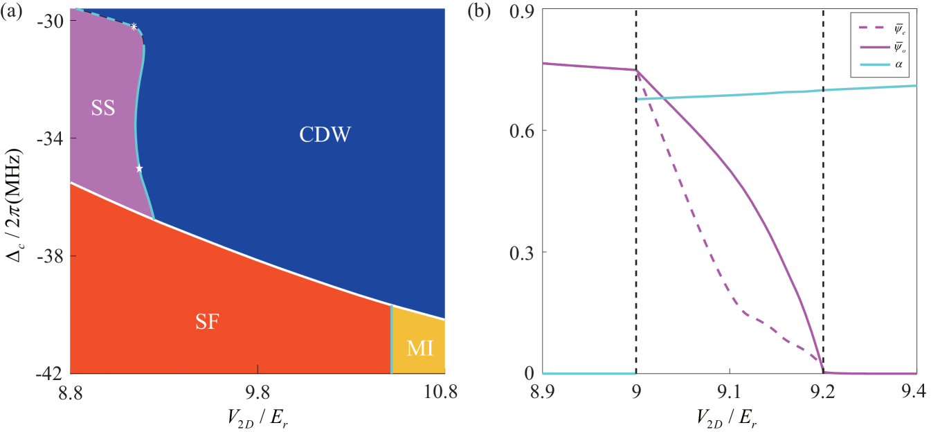
Figure 1: (a) Zero temperature phase diagram as a function
of the lattice depth and . There are four different phases
as shown in the phase diagram, which consists of a superfluid (SF) phase, a Mott insulator
(MI) state, a charge-density-wave (CDW)state and a supersolid (SS) phase.
The dashed and solid line separate the two distinct region, where two different types of Goldstone modes (type-I and type-II) were found in its single particle excitation, respectively. (b) Evolution of the different order parameters as a function of the lattice depth when MHz. is the recoil energy. Other parameters are chosen as , MHz, .
Path integral approach — In the following, we develop a strong-coupling expansion of the model Hamiltonian in Eq. (1),
which extends the treatment in Bose-Hubbard model Sengupta and Dupuis (2005), where both superfluid and Mott phases can be captured in the same time by this method. Through introducing the complex field , the thermodynamic properties of the system can be obtained from the partition function as a functional integral
with the action .
Here, is a imaginary time and is inverse temperature.
We then perform a Hubbard-Stratonovich transformation through introducing
the auxiliary field to decouple the intersite hopping
in the action and obtain
(3)
where represents the inverse hopping matrix. and are the action and partition function in the limit of . stands for averaging with . is the generation function
linking to connected local Green’s functions through the relation [25] ,
where means that all the fields share the same value of the
site index and . After doing a power expansion of to quartic order, we obtain that
(4)
where is the local Green’s function and is the two-particle vertex in
the local limit, i.e., (see details in SM). However, starting from the above action, it is inconvenient to calculate physical quantities, such as
the excitation spectrum or the momentum distribution. These difficulties can be circumvented through performing another Hubbard-Stratonovich transition to decouple
the hopping term Sengupta and Dupuis (2005). It is shown that the auxiliary field of this transformation
has the same correlation functions as the original boson field (see details in SM). Therefore, we can use the same notation for both fields. The partition function can thus
be expressed as
(5)
Integrating out the field in Eq. (5), the effective action can be obtained
(6)
where captures the amplitude of the boson-boson
interaction determined by the local two-particle vertex in its static limit (see details in SM).
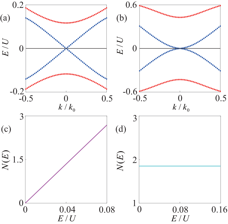
Figure 2: Excitation spectra for the two lowest-energy excitations (a) when
, MHz as indicated by ’’ in Fig. 1(a), (b) when , MHz as labelled by ’’ in Fig. 1(a). Other parameters are the same as Fig. 1. (c) (d) Density of states (DOS) defined in the main text for type I and type II Goldstone modes, respectively.
Phase diagram under the saddle-point approximation —
Starting from the above effective action, we first perform a saddle-point approximation
to determine the ground state of our proposed system. The saddle-point action derived from Eq. (6) can be expressed as
(7)
where and with and being
Fourier transforms of the single-particle Green’s function
and the two-particle vertex, respectively. The saddle-point value can be obtained from
minimizing and we obtain
(8)
(9)
where is the superfluid density of the pseudospin component and . By utilizing an iterative algorithm to solve a complete set of self-consistent equations (2), (8) and (9), superfluid order parameters for even and odd lattice sites and the mean value of cavity field can be determined. As defined in Eq. (2), characterizes the average imbalance between even and odd lattice sites, which can be used as the order parameter describing the CDW order.
We display the phase diagram as a function of the lattice depth and detuning in Fig. 1(a), to compare with the realistic experiments, such as the ETH experimental setup Landig et al. (2016). There are four different phases as shown in the phase
diagram, which consists of a superfluid (SF) phase, a Mott
insulator (MI) state, a charge-density-wave (CDW) state and a supersolid (SS) phase.
The difference among these four phases can be captured by order parameters defined
above, for example, as shown in Fig. 1(b). A SF phase is characterized by
finite and equal superfluid order parameters and vanishing even-odd imbalance indicated by . It is quite different in the SS phase, where a finite even-odd imbalance and nonzero superfluid order parameters are observed. In both MI and CDW states, superfluid order parameters vanish. However, the presence of a finite even-odd imbalance
distinguishes between MI and CDW states. The obtained phase diagram is consistent with other mean-field calculations Dogra et al. (2016); Chen et al. (2016). However, the path integral approach constructed here can provide a systematic
way beyond the mean-field approach for investigating the effect of high-order fluctuations. The unexpected results
driven by the fluctuations will be unveiled below.
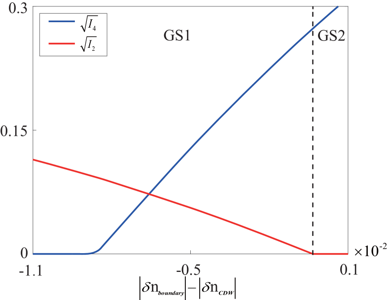
Figure 3: The coefficients and in (Eq. 12) as a function of density imbalance modulation when varying the system along the phase boundary between SS and CDW as shown in Fig. 1(a). The dashed line separates the regions with
type I and type II Goldstone modes, respectively. and describe the atom density imbalance between even and odd sites, when considering the system along the phase boundary and in CDW, respectively. Here is fixed at . Other parameters are chosen as the same in Fig. 1.
Manipulating Goldstone modes at the SS-CDW transition —
Since typically fluctuations will play a dominate role in determining physical properties at the critical region, to explore the unexpected results arising from
the fluctuations, we construct the critical theory describing the phase transition region as shown in Fig. 1(a). By performing both a spatial and a temporal gradient expansion of the action in Eq. (6), as well as the cumulant expansion in powers of
Sengupta and Dupuis (2005); Fisher et al. (1989); Faccioli and Salasnich (2018), the effective action can be rewritten as
(10)
where , ,
, .
and are the coefficients of the second-order temporal and spatial derivatives, respectively, which can be expressed in terms of the Green’s function (see
SM for details).
Next, we introduce to describe the fluctuations. After expanding the action in Eq. (10) to the quadric order of fluctuation fields , we get
(11)
where and the matrix elements of can be expressed as
Therefore, the single particle excitation spectrum at the critical region as shown in Fig. 1(a), can be obtained by solving
the equation .
Here we focus on the transition from SS to CDW. In SS phase, there are two superfluid order parameters for even and odd lattice sites, where the amplitude and phase of the order parameter emerge as two independent degree of freedoms, instead of being conjugate to each other. The phase fluctuation leads to the Goldstone mode, while the amplitude fluctuation leads to the Higgs mode. When further considering the coupling between even and odd lattice sites (hopping term between them), the two Higgs modes arising from the amplitude fluctuation will couple to each other and split into two new Higgs modes (two higher modes obtained from ). While the two Goldstone modes resulting from the phase fluctuation will also couple to each other and split into one gapless Goldstone mode associated with the overall phase plus a gapped mode linking to the relative phase .
At the transition from SS to CDW, we find the new feature of the lowest Goldstone mode excitation. Previous studies show that the slight modulation of density imbalance induced by the superradiant cavity light has a negligible effect on the single particle excitation spectrum Dogra et al. (2016). Here we firstly show that at the transition from SS to CDW, even such negligible modulation of density imbalance will result in a dramatic effect on the excitations. Distinct from the mean-field approach Dogra et al. (2016); Chen et al. (2016), such as employing
the Gutzwiller ansatz, the critical theory constructed in Eq. (10) can unveil the
dominate role of fluctuations. It is found that tuning the system along the phase boundary between SS and CDW as shown in Fig 1(a) can freely switch between
two types of Goldstone modes in its single particle excitation, i.e., type I and type II with odd and even power energy-momentum dispersion (as shown in Fig. 2), respectively.
To further understand the underlying physics, we analytically solve the equation and find that in the long wave limit the lowest single particle excitation (positive branch) can be approximately expressed as (See details in SM)
(12)
Therefore, the switching from type I to type II Goldstone modes can be achieved by changing the coefficients and . Around the transition from SS to CDW, it is shown that the quantum fluctuations make even the slight modulation of density imbalance play a dominant role in determining and . As shown in Fig. 3,
the slight modulation of density imbalance leads to two distinct regions: (I) , (II) and , which corresponds type I and type II Goldstone modes, respectively. To distinguish these two different types of Goldstone modes, we calculate the density of states (DOS) for the lowest single particle excitation
as , which is directly related to the Bragg spectroscopy signal Pippan et al. (2009). As shown in Fig. 2, with linear dispersion (type I), we find when . It is distinct from the quadratic dispersion (type II), where N(E) is a constant when . The experimental advances in the momentum-resolved Bragg spectroscopy in optical lattices Ernst et al. (2010b) make the detection of this signal accessible.
Conclusion —
By performing two successive Hubbard-Stratonovich transformations, we have
developed an effective field theory to study a bosonic lattice gas inside
a cavity in the strongly interacting regime. Through taking into account the quantum
fluctuations, we firstly find that the slight modulation of density imbalance, neglected in the previous studies, leads to dramatic changes of the behavior of low-energy excitations. The switching between type I and type II Goldstone modes can be driven along SS-CDW transition. Our findings would bridge the cavity light and strongly interacting quantum matters and may open up a new direction in this field.
Acknowledgement —
This work is supported by NSFC (Grant No.
12074305, 11774282, 11950410491), the National Key Research
and Development Program of China (2018YFA0307600), Cyrus Tang Foundation Young Scholar
Program and the Fundamental Research Funds for the Central Universities(H.W., S.L., M.A and B.L.) and by the AFOSR Grant No. FA9550-16-1-0006, the MURI-ARO Grant No. W911NF17-1-0323 through UC Santa Barbara, and the Shanghai Municipal Science and Technology Major Project through the Shanghai Research Center for Quantum Sciences (Grant No. 2019SHZDZX01) (W.V.L.). We also thank the HPC platform of Xi’An Jiaotong University, where our numerical calculations was performed.
References
Huang (1987)
K. Huang,
Statistical Machanics (John Wiley
and Sons,New York, 1987).
Nambu (1960)
Y. Nambu,
Phys. Rev. 117,
648 (1960).
Goldstone (1961)
J. Goldstone,
Nuovo Cimento 19,
154 (1961).
Nielsen and Chadha (1976)
H. B. Nielsen and
S. Chadha,
Nucl. Phys. B. 105,
445 (1976).
Bloch (1930)
F. Bloch, Z.
Phys. 61, 206
(1930).
Chubukov et al. (1994)
A. V. Chubukov,
S. Sachdev, and
J. Ye, Phys.
Rev. B. 49, 11919
(1994).
Podolsky and Sachdev (2012)
D. Podolsky and
S. Sachdev,
Phys. Rev. B. 86,
054508 (2012).
Ye and Jiang (2007)
J. Ye and
L. Jiang,
Phys. Rev. Lett. 98,
236802 (2007).
Ernst et al. (2010a)
P. T. Ernst,
S. Götze,
J. S. Krauser,
K. Pyka,
D. S. Lühmann,
D. Pfannkuche,
and
K. Sengstock,
Nature. Phys. 6,
56 (2010a).
Papp et al. (2008)
S. B. Papp,
J. M. Pino,
R. J. Wild,
S. Ronen,
C. E. Wieman,
D. S. Jin, and
E. A. Cornell,
Phys. Rev. Lett. 101,
135301 (2008).
Steinhauer et al. (2002)
J. Steinhauer,
R. Ozeri,
N. Katz, and
N. Davidson,
Phys. Rev. Lett. 88,
120407 (2002).
Stenger et al. (1999)
J. Stenger,
S. Inouye,
A. P. Chikkatur,
D. M. Stamper-Kurn,
D. E. Pritchard,
and W. Ketterle,
Phys. Rev. Lett. 82,
4569 (1999).
Stamper-Kurn et al. (1999)
D. M. Stamper-Kurn,
A. P. Chikkatur,
A. Görlitz,
S. Inouye,
S. Gupta,
D. E. Pritchard,
and W. Ketterle,
Phys. Rev. Lett. 83,
2876 (1999).
Kozuma et al. (1999)
M. Kozuma,
L. Deng,
E. W. Hagley,
J. Wen,
R. Lutwak,
K. Helmerson,
S. L. Rolston,
and W. D.
Phillips, Phys. Rev. Lett.
82, 871 (1999).
Yu et al. (2013)
Y.-X. Yu,
J. Ye, and
W.-M. Liu,
Scientific Reports 3,
3476 (2013).
Pan et al. (2020)
J.-S. Pan,
W. V. Liu, and
X.-J. Liu,
Phys. Rev. Lett. 125,
260402 (2020).
Greiner et al. (2002)
M. Greiner,
O. Mandel,
T. Esslinger,
T. W. Hänsch,
and I. Bloch,
Nature 415, 39
(2002).
Stöferle et al. (2004)
T. Stöferle,
H. Moritz,
C. Schori,
M. Köhl, and
T. Esslinger,
Phys. Rev. Lett. 92,
130403 (2004).
Sachdev (2011)
S. Sachdev,
Quantum Phase Transitions
(Cambridge University Press, 2011).
Endres et al. (2012)
M. Endres,
T. Fukuhara,
D. Pekker,
M. Cheneau,
P. Schau,
C. Gross,
E. Demler,
S. Kuhr, and
I. Bloch,
Nature 487,
454 (2012).
Pekker and Varma (2015)
D. Pekker and
C. M. Varma,
Annu. Rev. Condens. Matter. Phys.
6, 269 (2015).
Landig et al. (2016)
R. Landig,
L. Hruby,
N. Dogra,
M. Landini,
R. Mottl,
T. Donner, and
T. Esslinger,
Nature 532,
476 (2016).
Klinder et al. (2015)
J. Klinder,
H. Keßler,
M. R. Bakhtiari,
M. Thorwart, and
A. Hemmerich,
Phys. Rev. Lett. 115,
230403 (2015).
Dogra et al. (2016)
N. Dogra,
F. Brennecke,
S. D. Huber, and
T. Donner,
Phys. Rev. A. 94,
023632 (2016).
Freericks and Monien (1994)
J. K. Freericks
and H. Monien,
Europhys. Lett. 26,
545 (1994).
Freericks and Monien (1996)
J. K. Freericks
and H. Monien,
Phys. Rev. B. 53,
2691 (1996).
Sengupta and Dupuis (2005)
K. Sengupta and
N. Dupuis,
Phys. Rev. A. 71,
033629 (2005).
Chen et al. (2016)
Y. Chen,
Z. H. Yu, and
H. Zhai,
Phys. Rev. A. 93,
041601 (2016).
Baumann et al. (2010)
K. Baumann,
C. Guerlin,
F. Brennecke,
and
T. Esslinger,
Nature 464,
1301 (2010).
Fisher et al. (1989)
M. P. A. Fisher,
P. B. Weichman,
G. Grinstein,
and D. S.
Fisher, Phys. Rev. B
40, 546 (1989).
Faccioli and Salasnich (2018)
M. Faccioli and
L. Salasnich,
Symmetry 10
(2018).
Pippan et al. (2009)
P. Pippan,
H. G. Evertz,
and
M. Hohenadler,
Phys. Rev. A 80,
033612 (2009).
Ernst et al. (2010b)
P. T. Ernst,
S. Gtze,
J. S. Krauser,
K. Pyka,
D.-S. Lhmann,
D. Pfannkuche,
and
K. Sengstock,
Nature Physics 6,
56 (2010b).
Supplementary Material:
Manipulating Goldstone modes via the superradiant light in a bosonic lattice gas inside a cavity
S-1 Hopping term
The hopping term in Eq. (1) can be written as
(S1)
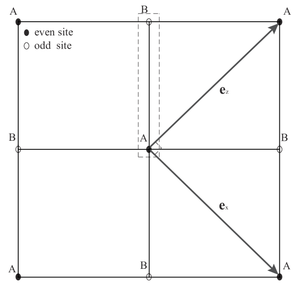
where stands for even and odd sites, respectively. is the hopping matrix and label the location of until cell as shown in Fig. S1. The hopping matrices can be expressed as
(S4)
(S7)
(S10)
Figure S1: Schematic picture of a two dimensional checkerboard lattice. Here A and B
stand for two different sites in one unit cell(even and odd sites), and are the primitive unit vectors.
In the momentum space, the hopping term can be written as
(S11)
where is the lattice constant and the band dispersion , .
S-2 Local single-particle and two-particle Green’s function
In the absence of hopping, i.e., , the local Hamiltonian can be defined from Eq.(1) as
with the energy detuning . Then, the local single-particle Green’s function can be calculated in the operator representation via the occupation number basis as
(S12)
where and is
the eigenbasis of the local Hamiltonian with eigenvalue .
After implementing the fourier transform, the above correlator can be expressed as
(S13)
In the low temperature limit , the exponential term in Eq. (S13) selects out the ground state of local Hamiltonian and contributions of other states are suppressed. Therefore, for instance, can be calculated as
(S14)
where and can be determined through minimizing the ground state energy .
In the same way, we can also obtain the local Green’s function as
(S15)
The two-particle Green’s function can be calculated in the similar way as
(S16)
where . To calculate the parameter in the static limit, we only consider the time average of . Then, the diagonal part can be calculated as
(S17)
with
Similarly, other diagonal part can also be calculated as follows
(S18)
In the similar way, we can obtain the off-diagonal part in the static limit as
(S19)
with
Up to this point, we have obtained the two-point and four-point correlators from
the local Hamiltonian. Then, in Eq. (6) of the main text can be determined by the two-particle vertex in the static limit, which can be written as
(S20)
where .
S-3 Double Hubbard-Stronovich transformation
The connected correlators of the original boson fields can be obtained from the generating function
(S21)
where are external sources and . Introducing the first Hubbard-Stratonovich transformation with auxiliary field ,
(S22)
After a shift , we obtain
(S23)
Integrating fields, we then obtain
(S24)
Next, applying the second Hubbard-Stratonovich transformation with auxiliary field ,
we obtain
(S25)
After integrating fields, we get
(S26)
From the above equation, we prove that is also the generating function of field, which is equal to the generating
function of orginal field. This proves that the connected correlators of are
the same as that of . Therefore, is identified with the original boson field . We can thus use the same notation for both fields.
S-4 Coefficients of the effective action at the critical region
To obtain the effective action at the critical region, we first rewrite the
action Eq.(6) in the main text in the momentum space as
(S27)
Next, we expand the inverse local single particle Green’s function and dispersion to the quadratic order in and
, respectively and obtain
(S28)
where , , ,
, , and .
Then, we can obtain the effective action Eq.(10) in the main text by transforming the action Eq.(S21) back to the real space.
S-5 the lowest single particle excitation
To find out the single particle excitation of the system, we analytically solve the equation . Therefore, the single particle excitation spectrum can be determined through the following relation
(S29)
where the coefficients are defined as , ,
,
,
,
, , ,
and with
, , . By analytically solving the above equation and expanding the energy dispersion to the quartic order of the momentum, the lowest single particle excitation (positive branch) can be approximately determined in the long-wave limit as