scale=1, angle=0, opacity=1, contents= \AtNextBibliography
![[Uncaptioned image]](https://cdn.awesomepapers.org/papers/fee88d65-6d69-4ff7-ab6c-e8b97495d104/x1.png)
Manipulator
Differential Kinematics
Part 1: Kinematics, Velocity, and Applications
Kinematics, derived from the Greek word for motion, is the branch of mechanics that studies the motion of a body, or a system of bodies, without considering mass or force. This two-part tutorial is about the kinematics of robot manipulators, and in that context, it is concerned with the relationship between the position of the robot’s joints and the pose of its end effector, as well as the relationships between various derivatives of those quantities. Kinematics is a fundamental concept in the study or application of robot manipulators, and our audience for Part 1 is students, practitioners or researchers encountering this topic for the first time, or looking for a concise refresher.
The relationship between end-effector pose and joint coordinates is encapsulated in the forward and inverse kinematics, and these are amongst the first concepts learned in this field. This tutorial begins with forward kinematics, but deliberately avoids the commonly-used Denavit-Hartenberg parameters which we feel confound pedagogy. Instead, we approach the problem using the elementary transform sequence (ETS) which is an intuitive, uncomplicated, and superior method for modelling a kinematic chain. Then we formulate the first-order differential kinematics which is the relationship between the velocity of the robot’s joints and the end-effector velocity. This relationship is expressed in terms of the manipulator Jacobian and is foundational for many fundamental robotic control algorithms, three of which we cover in this first article. Firstly, resolved-rate motion control – a simple algorithm that enables reactive, closed-loop and sensor-based velocity control of a manipulator. Secondly, numerical inverse kinematics (IK); an important planning tool that solves for joint coordinates which correspond to a specific manipulator pose. We introduce various methods that combine first-order differential kinematics and numerical optimisation and present a comprehensive experiment that compares the performance and characteristics of each numerical IK method. Thirdly, we introduce performance measures that describe a manipulator’s ability to move or exert force depending on its joint configuration.
Part 2 [1] of this tutorial provides a formulation of second and higher-order differential kinematics, introduces the manipulator Hessian, and illustrates advanced techniques, many of which improve the performance of techniques demonstrated in Part 1. These are useful topics that are not well covered in current textbooks.
We have provided Jupyter Notebooks to accompany this tutorial. The Notebooks are written in Python and use the Robotics Toolbox for Python, and the Swift Simulator [2] to provide full implementations of each concept, equation, and algorithm presented in this tutorial. The Notebooks use rich Markdown text and LaTeX equations to document and communicate key concepts. While not absolutely essential, for the most engaging and informative experience, we recommend working through the Jupyter Notebooks while reading this article. The Notebooks and setup instructions can be accessed at github.com/jhavl/dkt.
A serial-link manipulator, which we refer to as a manipulator, is the formal name for a robot that comprises a chain of rigid links and joints, it may contain branches, but it cannot have closed loops. Each joint provides one degree of freedom, which may be a prismatic joint providing translational freedom or a revolute joint providing rotational freedom. The base frame of a manipulator represents the reference frame of the first link in the chain, while the last link is known as the end-effector.
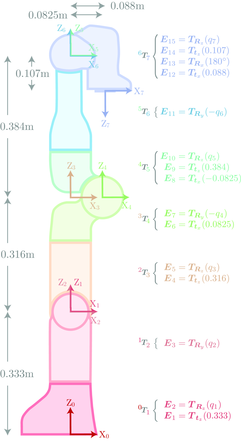
The elementary transform sequence (ETS), introduced in [3], provides a universal method for describing the kinematics of any manipulator. This intuitive and systematic approach can be applied with a simple walk through procedure. The resulting sequence comprises a number of elementary transforms – translations and rotations – from the base frame to the robot’s end-effector. An example of an ETS is displayed in Figure 1 for the Franka-Emika Panda in its zero-angle configuration.
The ETS is conceptually easy to grasp, and a reader can intuitively understand the kinematics of a manipulator at a glance. Additionally, the ETS avoids unnecessary complexity and frame assignment constraints of Denavit and Hartenberg (DH) notation [4] and allows joint rotation or translation about or along any axis. This makes the ETS a powerful tool for understanding robot kinematics and going forward we believe the ETS method should be considered the standard method for describing robot kinematics.
We use the notation of [5] where denotes a coordinate frame, and is a relative pose or rigid-body transformation of with respect to .
Forward Kinematics
The forward kinematics is the first and most fundamental relationship between the link geometry and robot configuration.
The forward kinematics of a manipulator provides a non-linear mapping
between the joint space and Cartesian task space, where is the vector of joint generalised coordinates, is the number of joints, and is a homogeneous transformation matrix representing the pose of the robot’s end-effector in the world-coordinate frame. The ETS model defines as the product of elementary transforms
| (1) |
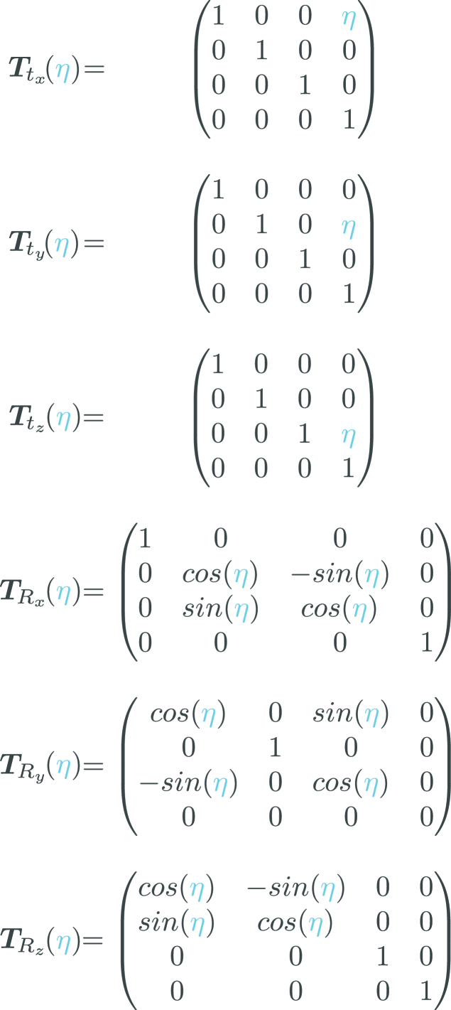
Each of the elementary transforms can be a pure translation along, or a pure rotation about the local x-, y-, or z-axis by an amount . Explicitly, each transform is one of the following
| (2) |
where each of the matrices are displayed in Figure 2 and the parameter is either a constant (translational offset or rotation) or a joint variable
| (3) |
and the joint variable is
| (4) |
where represents a joint angle, and represents a joint translation.
An ETS description does not require intermediate link frames, but it does not preclude their introduction. The convention we adopt is to place the frame immediately after the ETS term related to , as shown in Figure 1. The relative transform between link frames and is simply a subset of the ETS
| (5) |
where the function returns the index of the factor in the ETS expression, ( Forward Kinematics) in this case, which is a function of . For example, from Figure 1, for joint variable , .
Deriving the Manipulator Jacobian
First Derivative of a Pose
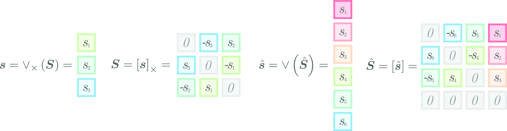
In the following sections, we use the skew and inverse skew operation as defined in Figure 3. Now consider the end-effector pose, which is a function of the joint coordinates given by ( Forward Kinematics). Its derivative with respect to time is
| (6) |
where each .
The information in is non-minimal, and redundant, as is the information in . We can write these respectively as
| (7) |
where , , and .
We will write the partial derivative in partitioned form as
| (8) |
where and , and then rewrite (6) as
and write a matrix equation for each non-zero partition
| (9) | ||||
| (10) |
where each term represents the contribution to end-effector velocity due to the motion of the corresponding joint.
Taking (10) first, we can simply write
| (11) |
where is the translational part of the manipulator Jacobian matrix.
Rotation rate is slightly more complex, but using the identity where is the angular velocity, and is a skew-symmetric matrix, we can rewrite (9) as
| (12) |
and rearrange to
This matrix equation therefore has only three unique equations so applying the inverse skew operator to both sides we have
| (13) |
where is the rotational part of the manipulator Jacobian.
Combining (11) and ( First Derivative of a Pose) we can write
| (14) |
which expresses end-effector spatial velocity in the world frame in terms of joint velocity and
| (15) |
is the manipulator Jacobian matrix expressed in the world-coordinate frame. The Jacobian expressed in the end-effector frame is
| (16) |
where is a rotation matrix representing the orientation of the end-effector in the world frame.
Combining (14) and (15) we write
| (17) |
which provides the derivative of the left side of ( Forward Kinematics). However, in order to compute (17), we need to first compute (8), that is .
First Derivative of an Elementary
Transform
Before differentiating the ETS to find the manipulator Jacobian, it is useful to consider the derivative of a single Elementary Transform.
Derivative of a Pure Rotation
The derivative of a rotation matrix with respect to the rotation angle is required when considering a revolute joint and can be shown to be
| (18) |
where the unit vector is the joint rotation axis.
The rotation axis can be recovered using the inverse skew operator
| (19) |
since , then .
For an ETS, we only need to consider the elementary rotations , , and as shown in Figure 2 which are embedded within , as , , and i.e. pure rotations with no translational component. We can show that the derivative of each elementary rotation with respect to a rotation angle is
| (20) | ||||
| (21) | ||||
| (22) |
If a joint’s defined positive rotation is a negative rotation about the axis, as is and in the ETS of the Panda shown in Figure 1, then is used to calculate the derivative.
Derivative of a Pure Translation
Consider the three elementary translations shown in Figure 2.
The derivative of a homogeneous transformation matrix with respect to translation is required when considering a prismatic joint. For an ETS, these translations are embedded in as , , and which are pure translations with zero rotational component. We can show that the derivative of each elementary translation with respect to a translation is
| (23) | ||||
| (24) | ||||
| (25) |
No changes are required if a joint’s defined positive translation is a negative translation along the axis.
The Manipulator Jacobian
Now we can calculate the derivative of an ETS. To find out how the joint affects the end-effector pose, apply the chain rule to ( Forward Kinematics)
| (26) |
The derivative of the elementary transform with respect to a joint coordinate in ( The Manipulator Jacobian) is obtained using one of (20), (21), or (22) for a revolute joint, or one of (23), (24), or (25) for a prismatic joint.
Using ( First Derivative of a Pose) with ( The Manipulator Jacobian) we can form the angular velocity component of the column of the manipulator Jacobian
| (27) |
where the operation is defined in Figure 4. Using (11) with ( The Manipulator Jacobian), the translational velocity component of the column of the manipulator Jacobian is
| (28) |
where the operation is defined in Figure 4.
Stacking the translational and angular velocity components, the column of the manipulator Jacobian becomes
| (29) |
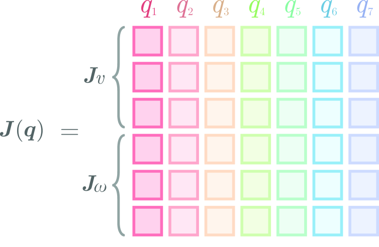
where the full manipulator Jacobian is
| (30) |
and we display a visualisation of the general structure of the manipulator Jacobian in Figure 5.
Fast Manipulator Jacobian
Calculating the manipulator Jacobian using (27) and (28) is easy to understand, but has time complexity – we can do better.
Expanding (27) using ( The Manipulator Jacobian) and simplifying using gives
| (31) |
where represents the transform from the base frame to frame as described by (5), and corresponds to one of the six elementary transform derivatives from equations (20)-(22) and (23)-(25).
In the case of a prismatic joint, will be a matrix of zeros which results in zero angular velocity. In the case of a revolute joint, the angular velocity is parallel to the axis of joint rotation.
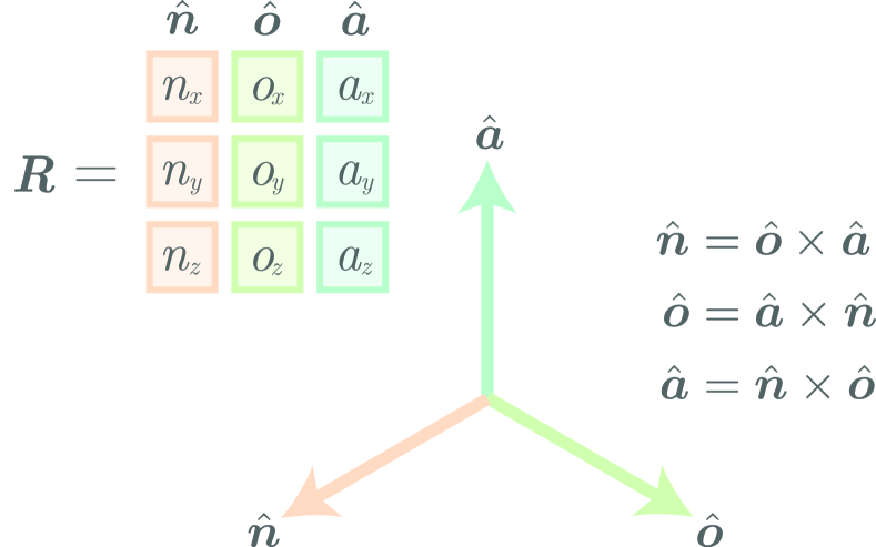
| (32) |
where are the columns of a rotation matrix as shown in Figure 6.
This simplification reduces the time complexity of computation of the manipulator Jacobian to .
Manipulator Jacobian
Applications
The manipulator Jacobian is widely used in robotic control algorithms and the remainder of this article details several applications of the manipulator Jacobian.
Resolved-Rate Motion Control
Resolved-rate motion control (RRMC), a direct application of the first-order differential equation we generated in (17), is a simple and elegant method to generate joint velocities which create a desired Cartesian end effector motion [6]. The ability to instantaneously change the end-effector velocity is at the heart of sensor-based reactive control. By “closing the loop” on sensory information a robot can adapt to changes in its environment as new knowledge is acquired by sensors. A well-known example is visual servoing, a technique that pairs robotic vision with RRMC to guide the manipulator to an image-based goal [7]. RRMC is also foundational for numerical inverse kinematics which we will visit in the next section [8, 9]. Of course, this introductory technique, while still highly relevant and powerful, can be extended and enhanced to improve robustness and consider constraints such as joint limits and environmental collisions [10, 11, 12, 13, 14, 15].
We first re-arrange (17)
| (35) |
which can only be solved when is square (and non-singular), which is when the robot has six degrees-of-freedom.
For redundant robots, there is no unique solution for (35). Consequently, the most common approach is to use the Moore-Penrose pseudoinverse
| (36) |
The pseudoinverse will return joint velocities with the minimum velocity norm of the possible solutions, although note an important caveat on mixed units described in Excurse 1.
Immediately from this, we can construct a primitive open-loop velocity controller. At each time step, we must calculate the manipulator Jacobian which is a function of the robot’s current configuration . Then we set to the desired spatial velocity of the end-effector.
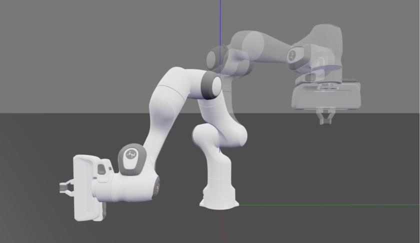
A more useful application of RRMC is to employ it in a closed-loop pose controller which we denote as position-based servoing (PBS). Using this method we can make the end-effector travel in a straight line, in the robot’s task space, towards some desired end-effector pose as displayed in Figure 7. The PBS scheme relies on an error vector which represents the translation and rotation from the end-effector’s current pose to the desired pose
| (37) |
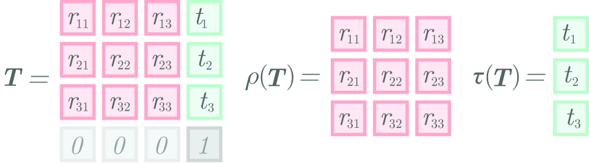
where the top three rows correspond to the translational error in the world frame, the bottom three rows correspond to the rotational error in the world frame, is the forward kinematics of the robot which represents the end-effector pose in the base frame of the robot, is the desired end-effector pose in the base frame of the robot ( denotes desired), and transforms a rotation matrix to its Euler vector equivalent [9]. The Euler vector is a form of angle-axis representation and specifies an axis of rotation and the angle of rotation about that axis.
List of Excurses 1 Inhomogeneous Units Vector norms can be problematic when they contain mixed units. For example and are non-homogeneous as they both combine translational and rotational units. For manipulators with mixed prismatic and revolute joints, so too does . Solutions include scaling [16] to ensure that the translational and rotational values have commensurate magnitude, or to consider translational and rotational components separately.
If is not a diagonal matrix then the Euler vector equivalent of is calculated as
| (38) |
where using the convention from Figure 4 we define and
| (39) |
If is a diagonal matrix then we use different formulas. For the case where then otherwise
| (40) |
To construct the PBS scheme we take the error term from (37) to set in (35) (or (36) for robots with 7+ degrees of freedom) at each time step
| (41) |
where is a proportional gain with units that controls the rate of convergence to the goal and is typically a diagonal matrix to set gains for each task-space DoF
| (42) |
where is the translational motion gain and is the rotational motion gain. The inverse of the gain, , corresponds to the time constant of the scheme. Note that since the error is in the base frame of the robot we must use the base-frame manipulator Jacobian in (35) or (36).
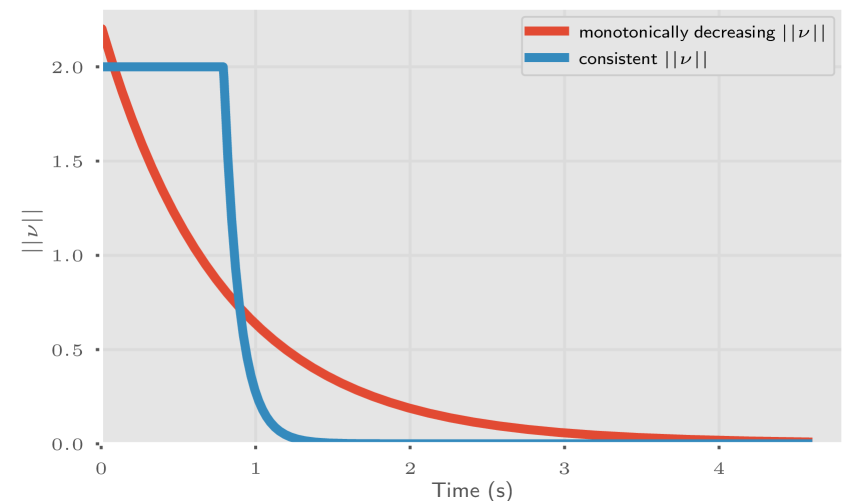
The control scheme we have just described will cause the error to asymptotically decrease to zero. For real applications, this is slow and impractical. We can improve this by increasing and and capping the end-effector velocity norm at some value , before stopping when the error norm drops below some value
| (43) |
This will cause to be consistent until is reached and subsequently asymptotically decreases to safely stop the robot. The effect of this is displayed in Figure 8 where has been set to 2.0. This approach involves combining mixed units, see Excurse 1.
This particular approach may cause unintuitive results as both and are non-homogeneous – they combine translational and rotational units. Therefore, a more intuitive approach would be to modify (43) to adjust the translational and angular velocity profiles separately. Alternate velocity profiles, such as a linearly decreasing velocity norm, are possible through modification of (43).
Although we have the safety mechanism of capping at , care must still be taken to not increase and without due consideration. Well-known problems caused by an excessive gain value, such as overshoot and system instability, may become apparent, especially on a real-world robot (which has non-modelled dynamics including flexibility, communication delay, and non-linearities).
For a reactive task, where a dynamic environment is causing the goal pose to change, simply update the desired end-effector pose in (37) at each time step, based on sensory information. A technique such as position-based visual servoing could be used to achieve this [7]. Refer to Notebook 3 where we use the Swift simulator to show this in action.
Numerical Inverse Kinematics
Inverse kinematics is the problem of determining the corresponding joint coordinates, given some end-effector pose. There are two approaches to solving inverse kinematics: analytical and numerical.
Analytical formulas must be pre-generated for a given manipulator and in some cases may not exist. The IKFast program provided as a part of OpenRAVE, pre-compiles analytic solutions for a given manipulator in optimised C++ code [17]. After this initial step, inverse kinematics can be computed rapidly, taking as little as 5 microseconds. However, analytic solutions generally can not optimise for additional criteria such as joint limits.
Numerical inverse kinematics use an iterative technique and can additionally consider extra constraints such as collision avoidance, joint limit avoidance, or manipulability [8, 9, 18]. In this section, we first construct a primitive numerical inverse kinematics solver, before showing how it can be improved using advanced optimisation techniques.
| Method | Searches Allowed | Iter. Allowed | Mean Iter. | Median Iter. | Infeasible Count | Infeasible % | Mean Searches | Max Searches |
|---|---|---|---|---|---|---|---|---|
| NR | 1 | 500 | 21.34 | 16.0 | 1093 | 10.93% | 1.0 | 1.0 |
| GN | 1 | 500 | 21.6 | 16.0 | 1078 | 10.78% | 1.0 | 1.0 |
| NR Pseudoinverse | 1 | 500 | 21.24 | 16.0 | 1100 | 11.0% | 1.0 | 1.0 |
| GN Pseudoinverse | 1 | 500 | 21.72 | 16.0 | 1090 | 10.9% | 1.0 | 1.0 |
| LM (Wampler ) | 1 | 500 | 20.1 | 14.0 | 934 | 9.34% | 1.0 | 1.0 |
| LM (Wampler ) | 1 | 500 | 29.84 | 17.0 | 529 | 5.29% | 1.0 | 1.0 |
| LM (Chan =1.0) | 1 | 500 | 16.58 | 14.0 | 1011 | 10.11% | 1.0 | 1.0 |
| LM (Chan =0.1) | 1 | 500 | 9.43 | 9.0 | 963 | 9.63% | 1.0 | 1.0 |
| LM (Sugihara ) | 1 | 500 | 20.54 | 15.0 | 1024 | 10.24% | 1.0 | 1.0 |
| LM (Sugihara ) | 1 | 500 | 17.01 | 14.0 | 1011 | 10.11% | 1.0 | 1.0 |
| NR | 100 | 30 | 30.16 | 18.0 | 0 | 0.0% | 1.47 | 25.0 |
| GN | 100 | 30 | 30.33 | 18.0 | 0 | 0.0% | 1.48 | 23.0 |
| NR Pseudoinverse | 100 | 30 | 30.27 | 18.0 | 0 | 0.0% | 1.47 | 20.0 |
| GN Pseudoinverse | 100 | 30 | 30.65 | 18.0 | 0 | 0.0% | 1.49 | 20.0 |
| LM (Wampler ) | 100 | 30 | 25.23 | 15.0 | 0 | 0.0% | 1.35 | 17.0 |
| LM (Wampler ) | 100 | 30 | 29.3 | 18.0 | 0 | 0.0% | 1.45 | 24.0 |
| LM (Chan =1.0) | 100 | 30 | 22.6 | 15.0 | 0 | 0.0% | 1.25 | 18.0 |
| LM (Chan =0.1) | 100 | 30 | 15.33 | 9.0 | 0 | 0.0% | 1.2 | 18.0 |
| LM (Sugihara ) | 100 | 30 | 26.49 | 16.0 | 0 | 0.0% | 1.35 | 18.0 |
| LM (Sugihara ) | 100 | 30 | 23.04 | 15.0 | 0 | 0.0% | 1.26 | 18.0 |
The Newton-Raphson (NR) method for inverse kinematics is remarkably similar to RRMC in a position-based servoing scheme. However, instead of sending joint velocities to the manipulator, the joint velocities update the configuration of a virtual manipulator until the goal pose is reached. To find the joint coordinates which correspond to some end-effector pose , the NR method seeks to minimise an error function
| (44) |
where is defined in (37), and is a diagonal weighting matrix which prioritises the corresponding error term. To achieve this, we iterate upon the following
| (45) |
With this approach, must be square (and non-singular) to be invertible and is therefore limited to manipulators with 6 joints.
When using the NR method, the initial joint coordinates should correspond to a non-singular manipulator pose, since it uses the manipulator Jacobian. When the problem is solvable, it converges very quickly. However, this method frequently fails to converge on the goal. We can improve the solvability of the problem and add compatibility with manipulators with greater than six joints, by using the Gauss-Newton (GN) method
| (46) | ||||
| (47) |
where is the base-frame manipulator Jacobian. If is non-singular, and , then (46) provides the pseudoinverse solution to (45). However, if is singular, (46) cannot be computed and the GN solution is infeasible.
Most linear algebra libraries (including the Python numpy library) implement the pseudoinverse using singular value decomposition, which is robust to singular matrices. Therefore, we can make both solvers more robust by using the pseudoinverse instead of the normal inverse in (45) and (46).
However, the computation is still unstable near singular points. We can further improve the solvability through the Levenberg-Marquardt (LM) method
| (48) | ||||
| (49) |
where is a diagonal damping matrix. The damping matrix ensures that is non-singular and positive definite. The performance of the LM method largely depends on the choice of . Wampler [19] proposed to be a constant, Chan and Lawrence [20] proposed a damped least-squares method with
| (50) |
where is a constant which does not have much influence on performance, and is the error value from (44) at time step . Sugihara [9] proposed
| (51) |
where , , and is the length of a typical link within the manipulator.
An important point to note is that the above methods are subject to local minima and in some cases will fail to converge on the solution. The choice of the initial joint configuration is important. An alternative approach is to re-start an IK problem with a new random after a few iterations rather than persist with a single attempt with iterations. This is a simple but effective method of performing a global search for the IK solution.
We display a comparison of IK methods presented in this tutorial in Table 1. Table 1 shows results for several IK algorithms trying to solve for randomly generated reachable end-effector poses using a six degree-of-freedom UR5 manipulator. We show each method initialised with a random valid and a maximum of 500 iterations to reach the goal before being declared infeasible. We also show each of the methods with 100 searches to reach the goal where a new search is initialised with a new random valid after 30 iterations. The iterations recorded for this method include the iterations from failed searches.
We have presented some useful IK methods but it is by no means an exhaustive list. Sugihara [9] provides a good comparison of many different numerical IK methods. In Part 2 of this tutorial, we explore advanced IK techniques which incorporate additional constraints into the optimisation.
Manipulator Performance Metrics
Manipulator performance metrics seek to quantify the performance of a manipulator in a given configuration. In this section, we explore two common manipulator performance metrics based on the manipulator Jacobian. A full survey of performance metrics can be found in [21]. It is important to note several considerations on how manipulator-based performance metrics should be used in practice. Firstly, the metrics are unitless, and the upper bound of a metric depends on the manipulator kinematic model (i.e. joint types and link lengths) and the units chosen to represent translation and orientation. Consequently, metrics computed for different manipulators are not directly comparable. Secondly, the manipulator Jacobian contains three rows corresponding to translational rates, and three rows corresponding to angular rates. Therefore, any metric using the whole Jacobian will produce a non-homogeneous result due to the mixed units. Depending on the manipulator scale, this can cause either the translational or rotational component to dominate the result. This problem also arises in manipulators with mixed prismatic and revolute joints. In general, the most intuitive use of performance metrics comes from using only the translational or rotational rows of the manipulator Jacobian (where the choice of which depends on the use case), and only using the metric on a manipulator comprising a single joint type [21].
Manipulability Index
The Yoshikawa manipulability index [22] is the most widely used and accepted performance metric [21]. The index is calculated as
| (52) |
where is either the translational or rotational rows of causing to describe the corresponding component of manipulability. Note that Yoshikawa used instead of in (52) but we describe it so due to limitations of Jacobian-based measures previously discussed. The scalar describes the volume of a 3-dimensional ellipsoid – if this ellipsoid is close to spherical, then the manipulator can achieve any arbitrary end-effector (translational or rotational depending on ) velocity. The ellipsoid is described by three radii aligned with its principal axes. A small radius indicates the robot’s inability to achieve a velocity in the corresponding direction. At a singularity, the ellipsoid’s radius becomes zero along the corresponding axis and the volume becomes zero. If the manipulator’s configuration is well conditioned, these ellipsoids will have a larger volume. Therefore, the manipulability index is essentially a measure of how easily a manipulator can achieve an arbitrary velocity.
Condition Number
The condition number of the manipulator Jacobian was proposed as a performance measure in [23]. The condition number is
| (53) |
where and are the maximum and minimum singular values of respectively. The condition number is a measure of velocity isotropy. A condition number close to means that the manipulator can achieve a velocity in a direction equally as easily as any other direction. However, a high condition number does not guarantee a high manipulability index where the manipulator may struggle to move in all directions.
Acknowledgments
We are grateful to the anonymous reviewers whose detailed and insightful comments have improved this article. This research was conducted by the Australian Research Council project number CE140100016, and supported by the QUT Centre for Robotics (QCR). We would also like to thank the members of QCR who provided valuable feedback and insights while testing this tutorial and associated Jupyter Notebooks.
Conclusions
In Part 1 of this tutorial, we have covered foundational aspects of manipulator differential kinematics. We first detailed a procedure for describing the kinematics of any manipulator and used this model to derive formulas for calculating the forward and first-order differential kinematics. We then detailed some applications unlocked by these formulas, including reactive motion control, inverse kinematics and methods which describe the performance of a manipulator at a given configuration. In Part 2, we explore second-order differential kinematics and detail how it can improve applications detailed in Part 1 while also unlocking new applications.
References
- [1] Jesse Haviland and Peter Corke “Manipulator Differential Kinematics: Part 2: Acceleration and Advanced Applications” In IEEE Robotics & Automation Magazine, 2023, pp. 2–12 DOI: 10.1109/MRA.2023.3270221
- [2] Peter Corke and Jesse Haviland “Not your grandmother’s toolbox–the Robotics Toolbox reinvented for Python” In 2021 IEEE international conference on robotics and automation (ICRA), 2021 IEEE
- [3] Peter I Corke “A simple and systematic approach to assigning Denavit–Hartenberg parameters” In IEEE transactions on robotics 23.3 IEEE, 2007, pp. 590–594
- [4] Richard S Hartenberg and Jacques Denavit “A kinematic notation for lower pair mechanisms based on matrices”, 1955
- [5] Peter Corke “Robotics, Vision and Control: fundamental algorithms in Python” Springer Nature, 2023 DOI: 10.1007/978-3-031-06468-5
- [6] D.. Whitney “Resolved Motion Rate Control of Manipulators and Human Prostheses” In IEEE Transactions on Man-Machine Systems 10.2, 1969, pp. 47–53
- [7] Seth Hutchinson, Gregory D Hager and Peter I Corke “A tutorial on visual servo control” In IEEE transactions on robotics and automation 12.5 IEEE, 1996, pp. 651–670
- [8] Pyung Chang “A closed-form solution for inverse kinematics of robot manipulators with redundancy” In IEEE Journal on Robotics and Automation 3.5, 1987, pp. 393–403
- [9] Tomomichi Sugihara “Solvability-unconcerned inverse kinematics by the Levenberg–Marquardt method” In IEEE Transactions on Robotics 27.5 IEEE, 2011, pp. 984–991
- [10] Jesse Haviland and Peter Corke “Maximising Manipulability During Resolved-Rate Motion Control” In arXiv preprint arXiv:2002.11901, 2020
- [11] D. Guo and Y. Zhang “Acceleration-Level Inequality-Based MAN Scheme for Obstacle Avoidance of Redundant Robot Manipulators” In IEEE Transactions on Industrial Electronics 61.12, 2014, pp. 6903–6914 DOI: 10.1109/TIE.2014.2331036
- [12] Jesse Haviland and Peter Corke “NEO: A Novel Expeditious Optimisation Algorithm for Reactive Motion Control of Manipulators” In IEEE Robotics and Automation Letters, 2021
- [13] Oussama Khatib “Real-time obstacle avoidance for manipulators and mobile robots” In Autonomous robot vehicles Springer, 1986, pp. 396–404
- [14] Dae-Hyung Park, Heiko Hoffmann, Peter Pastor and Stefan Schaal “Movement reproduction and obstacle avoidance with dynamic movement primitives and potential fields” In IEEE International Conference on Humanoid Robots, 2008
- [15] Nicolas Mansard, Olivier Stasse, Paul Evrard and Abderrahmane Kheddar “A versatile generalized inverted kinematics implementation for collaborative working humanoid robots: The stack of tasks” In 2009 International conference on advanced robotics, 2009, pp. 1–6 IEEE
- [16] Leo J Stocco, Septimiu E Salcudean and Farrokh Sassani “On the use of scaling matrices for task-specific robot design” In IEEE Transactions on Robotics and Automation 15.5 IEEE, 1999, pp. 958–965
- [17] Rosen Diankov “Automated Construction of Robotic Manipulation Programs”, 2010 URL: http://www.programmingvision.com/rosen_diankov_thesis.pdf
- [18] Arati S Deo and Ian D Walker “Adaptive non-linear least squares for inverse kinematics” In [1993] Proceedings IEEE International Conference on Robotics and Automation, 1993, pp. 186–193 IEEE
- [19] Charles W Wampler “Manipulator inverse kinematic solutions based on vector formulations and damped least-squares methods” In IEEE Transactions on Systems, Man, and Cybernetics 16.1 IEEE, 1986, pp. 93–101
- [20] Stephen K Chan and Peter D Lawrence “General inverse kinematics with the error damped pseudoinverse” In Proceedings. 1988 IEEE international conference on robotics and automation, 1988, pp. 834–839 IEEE
- [21] Sarosh Patel and Tarek Sobh “Manipulator performance measures-a comprehensive literature survey” In Journal of Intelligent & Robotic Systems 77.3 Springer, 2015, pp. 547–570
- [22] Tsuneo Yoshikawa “Manipulability of Robotic Mechanisms” In The International Journal of Robotics Research 4.2, 1985, pp. 3–9 DOI: 10.1177/027836498500400201
- [23] J Kenneth Salisbury and John J Craig “Articulated hands: Force control and kinematic issues” In The International journal of Robotics research 1.1 Sage Publications Sage UK: London, England, 1982, pp. 4–17