Mapping the Genetic-Imaging-Clinical Pathway with Applications to Alzheimer’s Disease
Dengdeng Yu
Department of Mathematics, University of Texas at Arlington
Linbo Wang
Department of Statistical Sciences, University of Toronto
Dehan Kong
Department of Statistical Sciences, University of Toronto
Hongtu Zhu
Department of Biostatistics, University of North Carolina, Chapel Hill
for the Alzheimer’s Disease Neuroimaging Initiative
111
Data used in preparation of this article were obtained from the Alzheimer’s Disease
Neuroimaging Initiative (ADNI) database (adni.loni.usc.edu). As such, the investigators within the ADNI contributed to the design and implementation of ADNI and/or provided data but did not participate in analysis or writing of this report. A complete listing of ADNI investigators can be found at: http://adni.loni.usc.edu/wp-content/uploads/how_to_apply/ADNI_Acknowledgement_List.pdf.
Abstract
Alzheimer’s disease is a progressive form of dementia that results in problems with memory, thinking, and behavior. It often starts with abnormal aggregation and deposition of amyloid and tau, followed by neuronal damage such as atrophy of the hippocampi, leading to Alzheimer’s Disease (AD). The aim of this paper is to map the genetic-imaging-clinical pathway for AD in order to delineate the genetically-regulated brain changes that drive disease progression based on the Alzheimer’s Disease Neuroimaging Initiative (ADNI) dataset. We develop a novel two-step approach to delineate the association between high-dimensional 2D hippocampal surface exposures and the Alzheimer’s Disease Assessment Scale (ADAS) cognitive score, while taking into account the ultra-high dimensional clinical and genetic covariates at baseline. Analysis results suggest that the radial distance of each pixel of both hippocampi is negatively associated with the severity of behavioral deficits conditional on observed clinical and genetic covariates. These associations are stronger in Cornu Ammonis region 1 (CA1) and subiculum subregions compared to Cornu Ammonis region 2 (CA2) and Cornu Ammonis region 3 (CA3) subregions. Supplementary materials for this article, including a standardized description of the materials available for reproducing the work, are available as an online supplement.
Keywords: 2D surface, behavioral deficits, confounders, hippocampus, variable selection.
1 Introduction
Alzheimer’s disease (AD) is an irreversible brain disorder that slowly destroys memory and thinking skills. According to World Alzheimer Reports (Gaugler et al., 2019), there are around million people worldwide living with Alzheimer’s disease and related dementia. The total global cost of Alzheimer’s disease and related dementia was estimated to be a trillion US dollars, equivalent to of global gross domestic product. Alzheimer’s patients often suffer from behavioral deficits including memory loss and difficulty of thinking, reasoning and decision making.
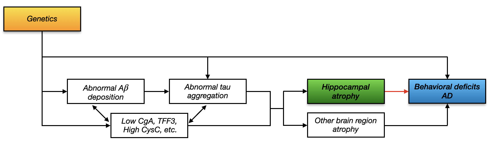
In the current model of AD pathogenesis, it is well established that deposition of amyloid plaques is an early event that, in conjunction with tau pathology, causes neuronal damage. Scientists have identified risk genes that may cause the abnormal aggregation and deposition of the amyloid plaques (e.g. Morishima-Kawashima and Ihara, 2002). The neuronal damage typically starts from the hippocampus and results in the first clinical manifestations of the disease in the form of episodic memory deficits (Weiner et al., 2013). Specifically, Jack Jr et al. (2010) presented a hypothetical model for biomarker dynamics in AD pathogenesis, which has been empirically and collectively supported by many works in the literature. The model begins with the abnormal deposition of amyloid (A) fibrils, as evidenced by a corresponding drop in the levels of soluble A-42 in cerebrospinal fluid (CSF) (Aizenstein et al., 2008). After that, neuronal damage begins to occur, as evidenced by increased levels of CSF tau protein (Hesse et al., 2001). Numerous studies have investigated how A and tau impact the hippocampus (e.g. Ferreira and Klein, 2011), known to be fundamentally involved in acquisition, consolidation, and recollection of new episodic memories (Frozza et al., 2018). In particular, as neuronal degeneration progresses, brain atrophy, which starts with hippocampal atrophy (Fox et al., 1996), becomes detectable by magnetic resonance imaging (MRI). Studies from recent years also found other important CSF proteins that may be related to hippocampal atrophy. For instance, the low levels of chromogranin A (CgA) and trefoil factor 3 (TFF3), and high level of cystatin C (CysC) are evidently associated with hippocampal atrophy (Khan et al., 2015; Paterson et al., 2014). Indeed, the impact of protein concentration on behavior can also be through atrophy of other brain regions. For example, there exists potential entorhinal tau pathology on episodic memory decline (Maass et al., 2018). As sufficient brain atrophy accumulates, it results in cognitive symptoms and impairment. This process of AD pathogenesis is summarized by the flow chart in Figure 1. Note that it is still debatable how A and tau interact with each other as mentioned by Jack Jr et al. (2013); Majdi et al. (2020); however, it is evident that A may still hit a biomarker detection threshold earlier than tau (Jack Jr et al., 2013). In addition, as noted by Hampel et al. (2018), it is likely that highly complex interactions exist between A as well as tau, and the cholinergic system. For instance, the association has been found between CSF biomarkers of amyloid and tau pathology in AD (Remnestål et al., 2021). It has also been found that other factors, such as dysregulation and dysfunction of the Wnt signaling pathway, may also contribute to A and tau pathologies (Ferrari et al., 2014). In addition, the M1 and M3 subtypes of muscarinic receptors increase amyloid precursor protein production via the induction of the phospholipase C/protein kinase C pathway and increase BACE expression in AD brains (Nitsch et al., 1992).
The aim of this paper is to map the genetic-imaging-clinical (GIC) pathway for AD, which is the most important part of the hypothetical model of AD pathogenesis in Figure 1. Histological studies have shown that the hippocampus is particularly vulnerable to Alzheimer’s disease pathology and has already been considerably damaged at the first occurrence of clinical symptoms (Braak and Braak, 1998). Therefore, the hippocampus has become a major focus in Alzheimer’s studies (De Leon et al., 1989). Some neuroscientists even conjecture that the association between hippocampal atrophy and behavioral deficits may be causal, because the former destroys the connections that help the neuron communicate and results in a loss of function (Watson, 2019). We are interested in delineating the genetically-regulated hippocampal shape that drives AD related behavioral deficits and disease progression.
To map the GIC pathway, we extract clinical, imaging, and genetic variables from the Alzheimer’s Disease Neuroimaging Initiative (ADNI) study as follows. First, we use the Alzheimer’s Disease Assessment Scale (ADAS) cognitive score to quantify behavioral deficits, for which a higher score indicates more severe behavioral deficits. Second, we characterize the exposure of interest, hippocampal shape, by the hippocampal morphometry surface measure, summarized as two matrices corresponding to the left/right hippocampi. Each element of the matrices is a continuous-valued variable, representing the radial distance from the corresponding coordinate on the hipppocampal surface to the medial core of the hippocampus. Compared with the conventional scalar measure of hippocampus shape (Jack et al., 2003), recent studies show that the additional information contained in the hippocampal morphometry surface measure is valuable for Alzheimer’s diagnosis (Thompson et al., 2004). For example, Li et al. (2007) showed that the surface measures of the hippocampus could provide more subtle indexes compared with the volume differences in discriminating between patients with Alzheimer’s and healthy control subjects. In our case, with the 2D matrix radial distance measure, one may investigate how local shapes of hippocampal subfields are associated with the behavioral deficits. Third, the ADNI study measures ultra-high dimensional genetic covariates and other demongraphic covariates at baseline. There are more than million genetic variants per subject.
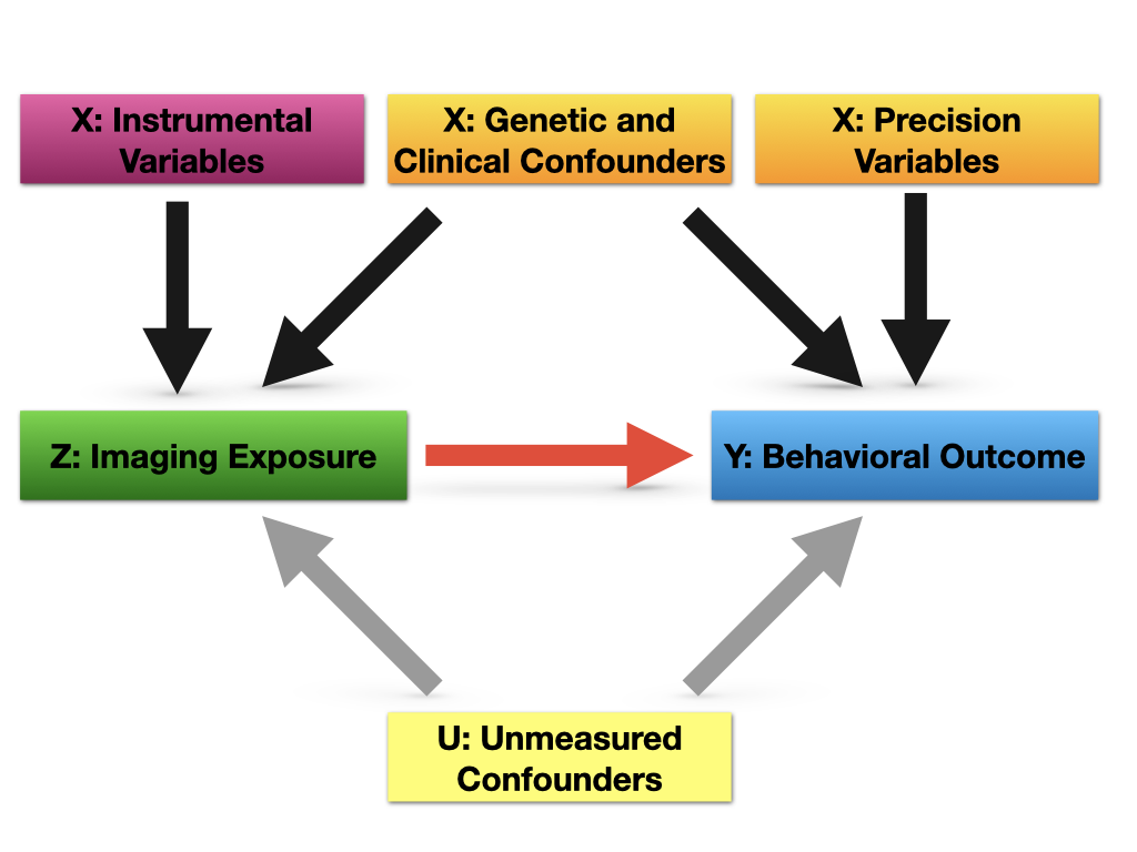
The special data structure of the ADNI data application presents new challenges for statistically mapping the GIC pathway. First, unlike conventional statistical analysis that deals with scalar exposure, our exposure of interest is represented by high-dimensional 2D hippocampal imaging measures. Second, the dimension of baseline covariates, which are also potential confounders, is much larger than the sample size. Recently there have been many developments for confounder selection, most of which are in the causal inference literature. Studies show inclusion of the variables only associated with exposure but not directly with the outcome except through the exposure (known as instrumental variables) may result in loss of efficiency in the causal effect estimate (e.g. Schisterman et al., 2009), while inclusion of variables only related to the outcome but not the exposure (known as precision variables) may provide efficiency gains (e.g. Brookhart et al., 2006); see Shortreed and Ertefaie (2017); Richardson et al. (2018); Tang et al. (2021) and references therein for an overview.
When a large number of covariates are available, the primary difficulty for mapping the GIC pathway is how to include all the confounders and precision variables, while excluding all the instrumental variables and irrelevant variables (not related to either outcome or exposure). We develop a novel two-step approach to estimate the conditional association between the high-dimensional 2D hippocampal surface exposure and the Alzheimer’s behaviorial score, while taking into account the ultra-high dimensional baseline covariates. The first step is a fast screening procedure based on both the outcome and exposure models to rule out most of the irrelevant variables. The use of both models in screening is crucial for both computational efficiency and selection accuracy, as we will show in detail in Sections 3.3 and 3.4. The second step is a penalized regression procedure for the outcome generating model to further exclude instrumental and irrelevant variables, and simultaneously estimate the conditional association. Our simulations and ADNI data application demonstrate the effectiveness of the proposed procedure.
Our analysis represents a novel inferential target compared to recent developments in imaging genetics mediation analysis (Bi et al., 2017). Although we consider a similar set of variables and structure among these variables as illustrated later in Figure 2, our goal is to estimate the conditional association of hippocampal shape with behavioral deficits. In contrast, in mediation analysis, researchers are often interested in the effects of genetic factors on behavioral deficits, and how those are mediated through hippocampus. Direct application of methods developed for imaging genetics mediation analysis to our problem may select genetic factors that are confounders affecting both hippocampal shape and behavioral deficits. In comparison, we aim to include precision variables in the adjustment set as they may improve efficiency.
The rest of the article is organized as follows. Section 2 includes a detailed data and problem description. We introduce our models and a two-step variable selection procedure in Section 3. We analyze the ADNI data and estimate the association between hippocampal shape and behavioral deficits conditional on observed clinical and genetic covariates in Section 4. Simulations are conducted in Section 5 to evaluate the finite-sample performance of the proposed method. We finish with a discussion in Section 6. The theoretical properties of our procedure are included in Section 15 in the supplementary material.
2 Data and problem description
Understanding how human brains work and how they connect to human behavior is a central goal in medical studies. In this paper, we are interested in studying whether and how hippocampal shape is associated with behavioral deficits in Alzheimer’s studies. We consider the clinical, genetic, imaging and behavioral measures in the ADNI dataset. The outcome of interest is the Alzheimer’s Disease Assessment Scale cognitive score observed at 24th month after baseline measurements. The Alzheimer’s Disease Assessment Scale cognitive 13 items score (ADAS-13) (Mohs et al., 1997) includes 13 items: word recall task, naming objects and fingers, following commands, constructional praxis, ideational praxis, orientation, word recognition task, remembering test directions, spoken language, comprehension, and word-finding difficulty, delayed word recall and a number cancellation or maze task. A higher ADAS score indicates more severe behavioral deficits.
The exposure of interest is the baseline 2D surface data obtained from the left/right hippocampi. The hippocampus surface data were preprocessed from the raw MRI data, where the detailed preprocessing steps are included in Section 9.1 of the supplementary material. After preprocessing, we obtained left and right hippocampal shape representations as two matrices. The imaging measurement at each pixel is an absolute metric, representing the radial distance from the pixel to the medial core of the hippocampus. The unit for the measurement is in millimeters.
In the ADNI data, there are millions of observed covariates that one may need to adjust for, including the whole genome sequencing data from all of the 22 autosomes. We have included detailed genetic preprocessing techniques in Section 9.2 of the supplementary material. After preprocessing, bi-allelic markers (including SNPs and indels) of subjects were retained in the data analysis.
We excluded those subjects with missing hippocampus shape representations, baseline intracranial volume (ICV) information or ADAS-13 score observed at Month 24, after which there are subjects left. Our aim is to estimate the association between the hippocampal surface exposure and the ADAS-13 score conditional on clinical measures including age, gender and length of education, ICV, diagnosis status, and bi-allelic markers.
3 Methodology
3.1 Basic set-up
Suppose we observe independent and identically distributed samples generated from , where has support . Here is a 2D-image continuous exposure, is a continuous outcome of interest, and denotes a vector of ultra-high dimensional genetic (and clinical) covariates, where we assume . We are interested in characterizing the association between the 2D exposure and outcome conditional on the observed covariates .
Denote . Without loss of generality, we assume that has been standardized for every , and and have been centered. To map the GIC pathway, we assume the following linear equation models:
| (1) | |||||
| (2) |
In (1), the matrix is the main parameter of interest, representing the association between the 2D imaging treatment and the behavioral outcome , represents the association between the -th observed covariate and the behavioral outcome , and and are random errors that may be correlated. The inner product between two matrices is defined as , where is a vectorization operator that stacks the columns of a matrix into a vector. Model (2), previously introduced in Kong et al. (2020), specifies the relationship between the 2D imaging exposure and the observed covariates. The is a coefficient matrix characterizing the association between the th covariate and the 2D imaging exposure , and is a matrix of random errors with mean . The symbol “” denotes element-wise multiplication. Define and , where we assume and ; here and represent the number of elements in and respectively.
To estimate , the first step is to perform variable selection in models (1) and (2). For all the covariates , we group them into four categories. Let , and denote the indices of confounders, i.e. variables associated with both the outcome and the exposure; denotes the indices of precision variables, i.e. predictors of the outcome, but not the exposure; denotes the indices of instrumental variables, i.e. covariates that are only associated with the exposure but not directly with the outcome except through the exposure; denotes the indices of irrelevant variables, i.e. covariates that are not related to the outcome or the exposure. Mathematically speaking, , , and . The relationships among different types of , and are shown in Figure 2, where denotes possible unmeasured confounders. Since we are interested in characterizing the association between and conditional on , further discussion of will be omitted for the remainder of the paper.
When there are no unobserved confounders , the estimate of has underlying causal interpretations. In this case, the ideal adjustment set includes all confounders to avoid bias and all precision variables to increase statistical efficiency, while excluding instrumental variables and irrelevant variables (Brookhart et al., 2006; Shortreed and Ertefaie, 2017). Although we are studying the conditional association rather than the causal relationship due to the possible unobserved confounding, our target adjustment set remains the same. In other words, we aim to retain all covariates from , while excluding covariates from .
3.2 Naive screening methods
To find the nonzero ’s, a straightforward idea is to consider a penalized estimator obtained from the outcome generating model (1), where one imposes, say Lasso penalties, on ’s. However, this is computationally infeasible in our ADNI data application as the number of baseline covariates is over million. Consequently, it is important to employ a screening procedure (e.g. Fan and Lv, 2008) to reduce the model size. To find covariates ’s that are associated with the outcome conditional on the exposure , one might consider a conditional screening procedure for model (1) (Barut et al., 2016). Specifically, one can fit the model for each , obtain marginal estimates of ’s and then sort the ’s for screening. This procedure works well if the exposure variable is of low dimension as one only needs to fit low dimensional ordinary least squares (OLS) times. However, in our ADNI data application, the imaging exposure is of dimension . As a result, one cannot obtain an OLS estimate since . Thus, to apply the conditional sure independence screening procedure to our application, one may need to solve a penalized regression problem for each , such as , where is a penalty of . In theory, for each one can obtain the estimates , and then rank the ’s. However, this is computationally prohibitive in the ADNI data with . First, the penalized regression problem is much slower to solve compared to the OLS. Second, selection of the tuning parameter based on grid search substantially increases the computational burden.
Alternatively one may apply the marginal screening procedure of Fan and Lv (2008) to model (1). Specifically, one may solve the following marginal OLS on each by ignoring the exposure : . The marginal OLS estimate has a closed form , and one can rank ’s for screening. Specifically, the selected sub-model is defined as , where is a threshold. Computationally, it is much faster than conditional screening for model (1) as we only need to fit one dimensional OLS for times. However, this procedure is likely to miss some important confounders. To see this, plugging model (2) into (1) yields
Even in the ideal case when ’s are orthogonal for , is not a good estimate of because of the bias term . Thus, we may miss some nonzero ’s in the screening step if and are of similar magnitudes but opposite signs. We illustrate this point in Figures 5 in Section 5, in which cases the conventional marginal screening on (1) fails to capture some of the important confounders.
3.3 Joint screening
To overcome the drawbacks of the estimation methods discussed in Section 3.2, we develop a joint screening procedure, specifically for our ADNI data application. The procedure is not only computationally efficient, but can also select all the important confounders and precision variables with high probability. The key insight here is that although we are interested in selecting important variables in the outcome generating model, this can be done much more efficiently by incorporating information from the exposure model. Specifically, let be the marginal OLS estimate in model (2) for . Following Kong et al. (2020), the important covariates in model (2) can be selected by , where is the operator norm of a matrix and is a threshold.
We define our joint screening set as . Intuitively, most important confounders and precision variables are contained in the set . The only exceptions are the covariates for which both and are of similar magnitudes but opposite signs. On the other hand, these will be included in and hence, along with instrumental variables with large . In Section 15 of the supplementary material, we show that with properly chosen and , the joint screening set includes the confounders and precision variables with high probability: as . In practice, we recommend choosing and such that , where is the smallest integer such that . We set them to be of equal sizes following the convention that the size of screening set is determined only by the sample size (Fan and Lv, 2008), which is the same for and . Depending on the prior knowledge about the sizes and signal strengths of confounding, precision and instrumental variables, the sizes of and may be chosen differently. In the simulations and real data analyses, we conduct sensitivity analyses by varying the relative sizes of and .
In general, the set includes not only confounders and precision variables in , but also instrumental variables in and a small subset of the irrelevant variables . Nevertheless, the size of is greatly reduced compared to that of all the observed covariates. This makes it feasible to perform the second step procedure, a refined penalized estimation of based on the covariates .
3.4 Blockwise joint screening
Linkage disequilibrium (LD) is a ubiquitous biological phenomenon where genetic variants present a strong blockwise correlation (LD) structure (Wall and Pritchard, 2003). If all the SNPs of a particular LD block are important but with relatively weak signals, they may be missed by the screening procedure described in Section 3.3. To appropriately utilize LD blocks’ structural information to select those missed SNPs, we develop a modified screening procedure described below.
Suppose that can be divided into discrete haplotype blocks: regions of high LD that are separated from other haplotype blocks by many historical recombination events (Wall and Pritchard, 2003). Let the index set of each non-overlapping block be with . For we define
where is the indicator function of an event. We also define
We propose to use the new set , rather than , to select important covariates. Intuitively, when , is much more easily selected compared with by . However, suppose that and , with only a small proportion of in having , whereas a large proportion of in has . It may well be the case that , meaning that can be selected more easily than by . In addition, as is not a good estimate of due to the bias term , is not a good estimate of either. Therefore, some with nonzero may not be included in . Nevertheless, they will be included in and hence .
Theoretically, when , , and are chosen properly, as ; see Theorem 3 in Section 15 of the supplementary material. In practice, we recommend choosing , , and , such that , where is the smallest integer such that . The threshold here is twice the threshold what we suggested in Section 3.3 since we unionize two additional sets.
3.5 Second-step estimation
In this step, we aim to estimate by excluding the instrument variables and irrelevant variables in from (or ) and keeping the other covariates. This can be done by solving the following optimization problem:
| (3) |
Denote the solution to the above optimization problem. The Lasso penalty on is used to exclude instrumental and irrelevant variables in , whose corresponding coefficients ’s are zero. The nuclear norm penalty , defined as the sum of all the singular values of a matrix, is used to achieve a low-rank estimate of , where the low-rank assumption in estimating 2D structural coefficients is commonly used in the literature (Zhou and Li, 2014; Kong et al., 2020). For tuning parameters, we use five-fold cross validation based on two-dimensional grid search, and select and using the one standard error rule (Hastie et al., 2009).
4 ADNI data applications
We use the data obtained from the ADNI study (adni.loni.usc.edu). The data usage acknowledgement is included in Section 8 of the supplement material. As described in Section 2, we include subjects from the ADNI1 study. The exposure of interest is the baseline 2D hippocampal surface radial distance measures, which can be represented as a matrix for each part of the hippocampus. The outcome of interest is the ADAS-13 score observed at Month 24. The average ADAS-13 score is with standard deviation . The covariates to adjust for include bi-allelic markers as well as clinical covariates, including age, gender and education length, baseline intracranial volume (ICV), and baseline diagnosis status. The average age is years old with standard deviation years, and the average education length is years with standard deviation years. Among all the subjects, were female. The average ICV was with standard deviation . There were ( at Month 24) cognitive normal patients, ( at Month 24) patients with mild cognitive impairment (MCI), and ( at Month 24) patients with AD at the baseline. Studies have shown that age and gender are the main risk factors for Alzheimer’s disease (Vina and Lloret, 2010; Guerreiro and Bras, 2015) with older people and females more likely to develop Alzheimer’s disease. Multiple studies have also shown that prevalence of dementia is greater among those with low or no education (Zhang et al., 1990). On the other hand, age, gender and length of education have been found to be strongly associated with the hippocampus (Van de Pol et al., 2006; Jack et al., 2000; Noble et al., 2012). Previous studies (Sargolzaei et al., 2015) suggest that the ICV is an important measure that needs to be adjusted for in studies of brain change and AD. In addition, the baseline diagnosis status may help explain the baseline hippocampal shape and the AD status at Month 24. Therefore, we consider age, gender, education length, baseline ICV and baseline diagnosis status as part of the confounders, and adjust for them in our analysis. In addition, we also adjust for population stratification, for which we use the top five principal components of the whole genome data. As both left and right hippocampi have 2D radial distance measures and the two parts of hippocampi have been found to be asymmetric (Pedraza et al., 2004), we apply our method to the left and right hippocampi separately.
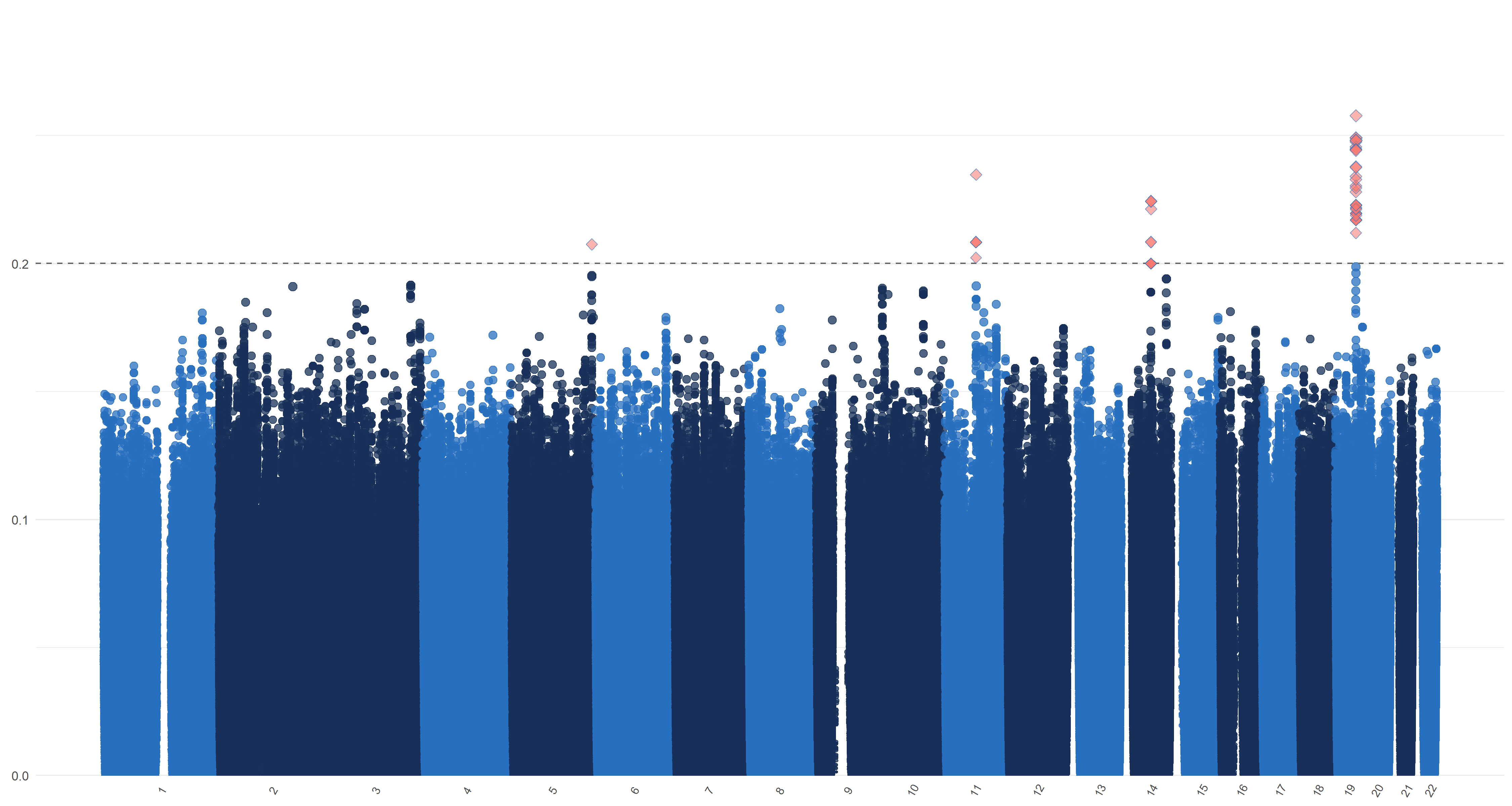
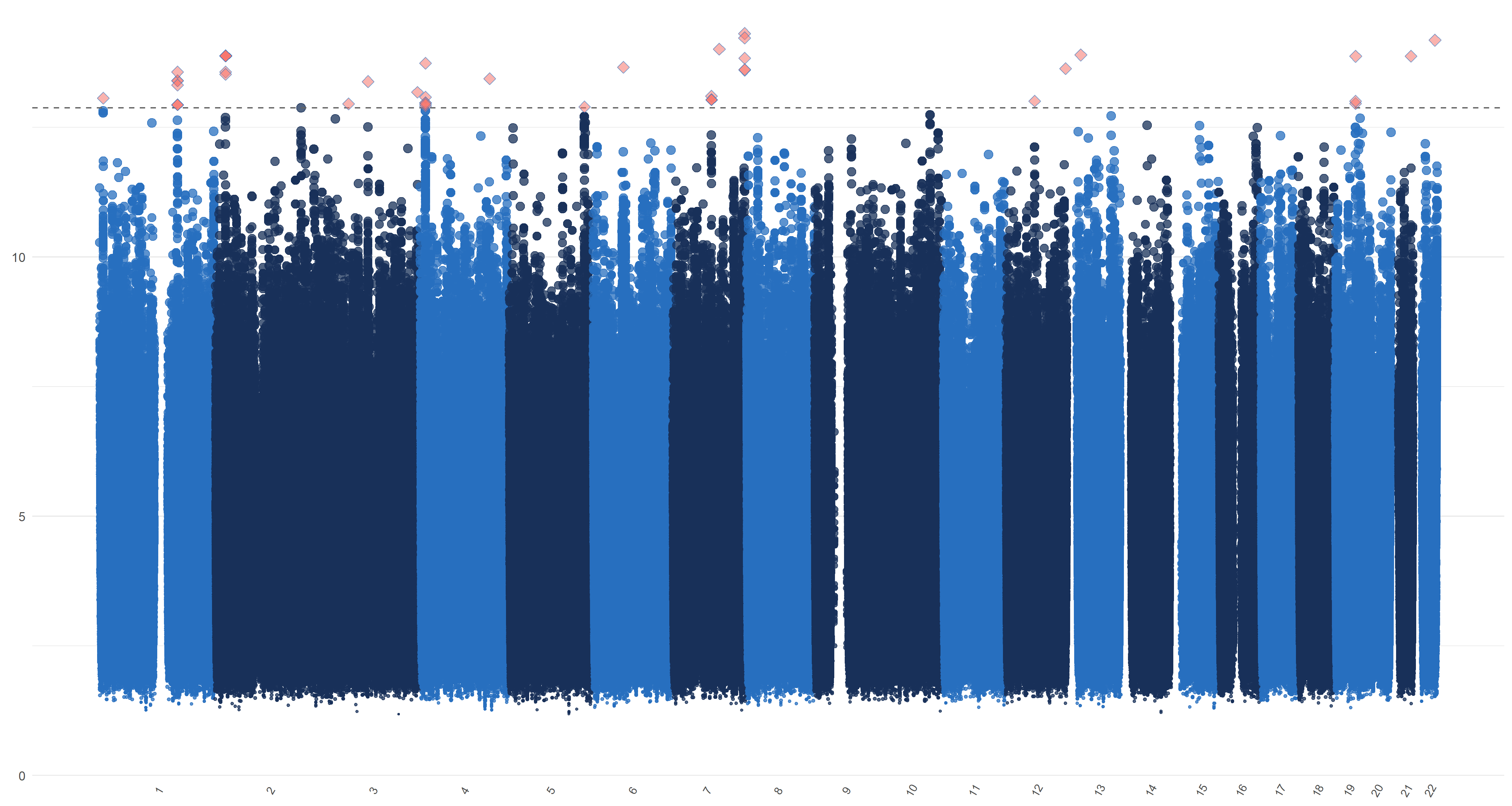
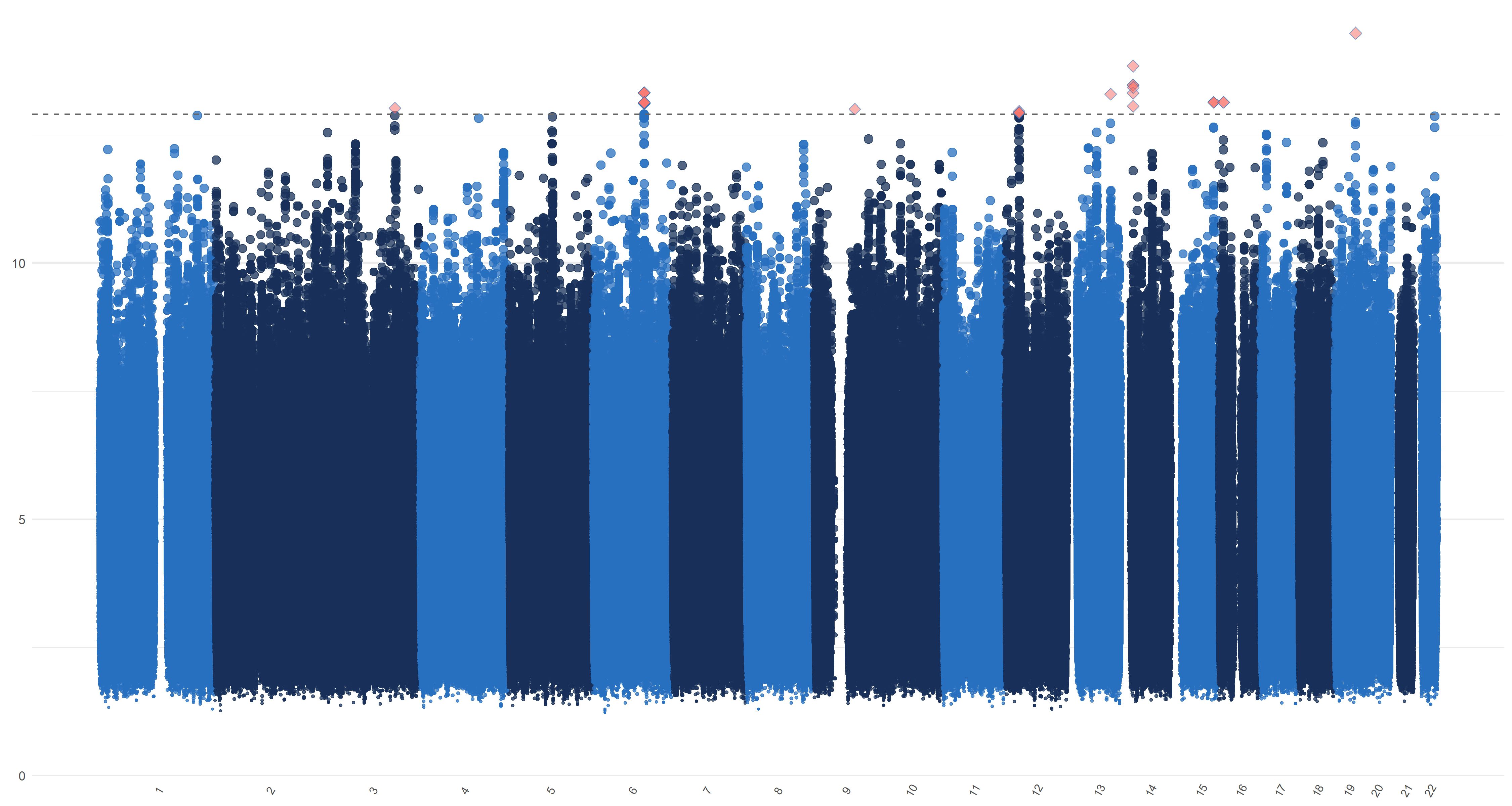
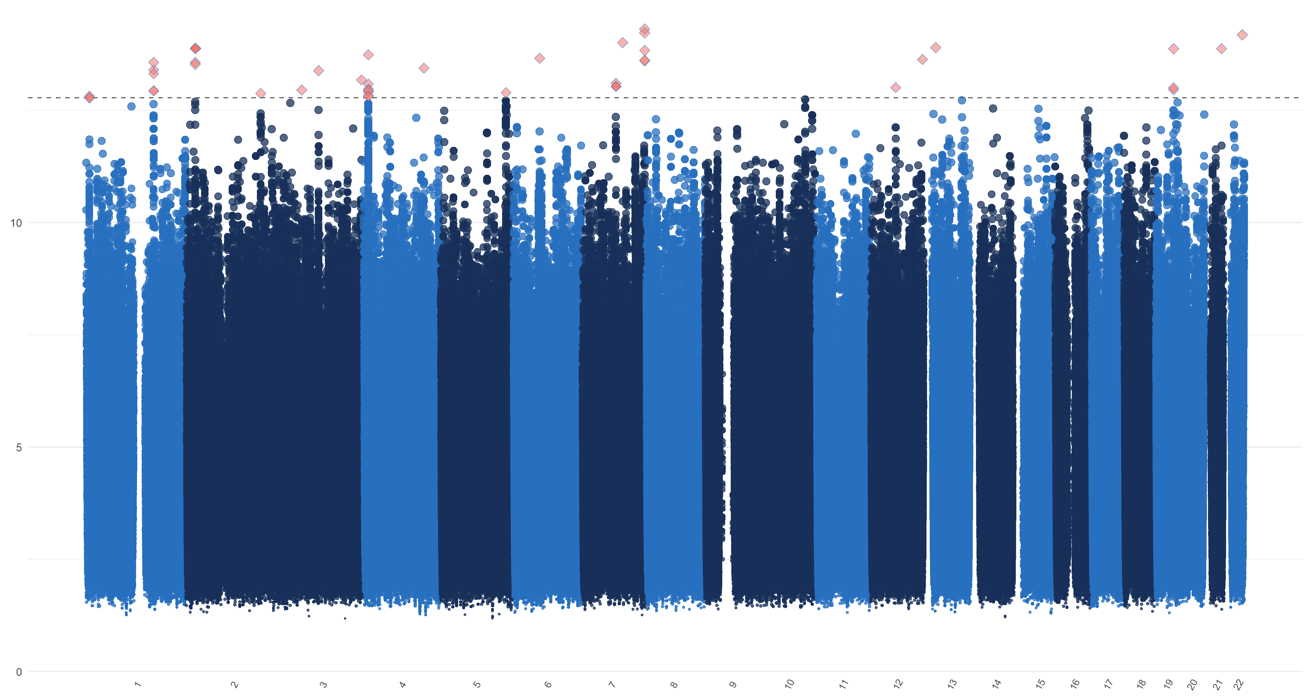
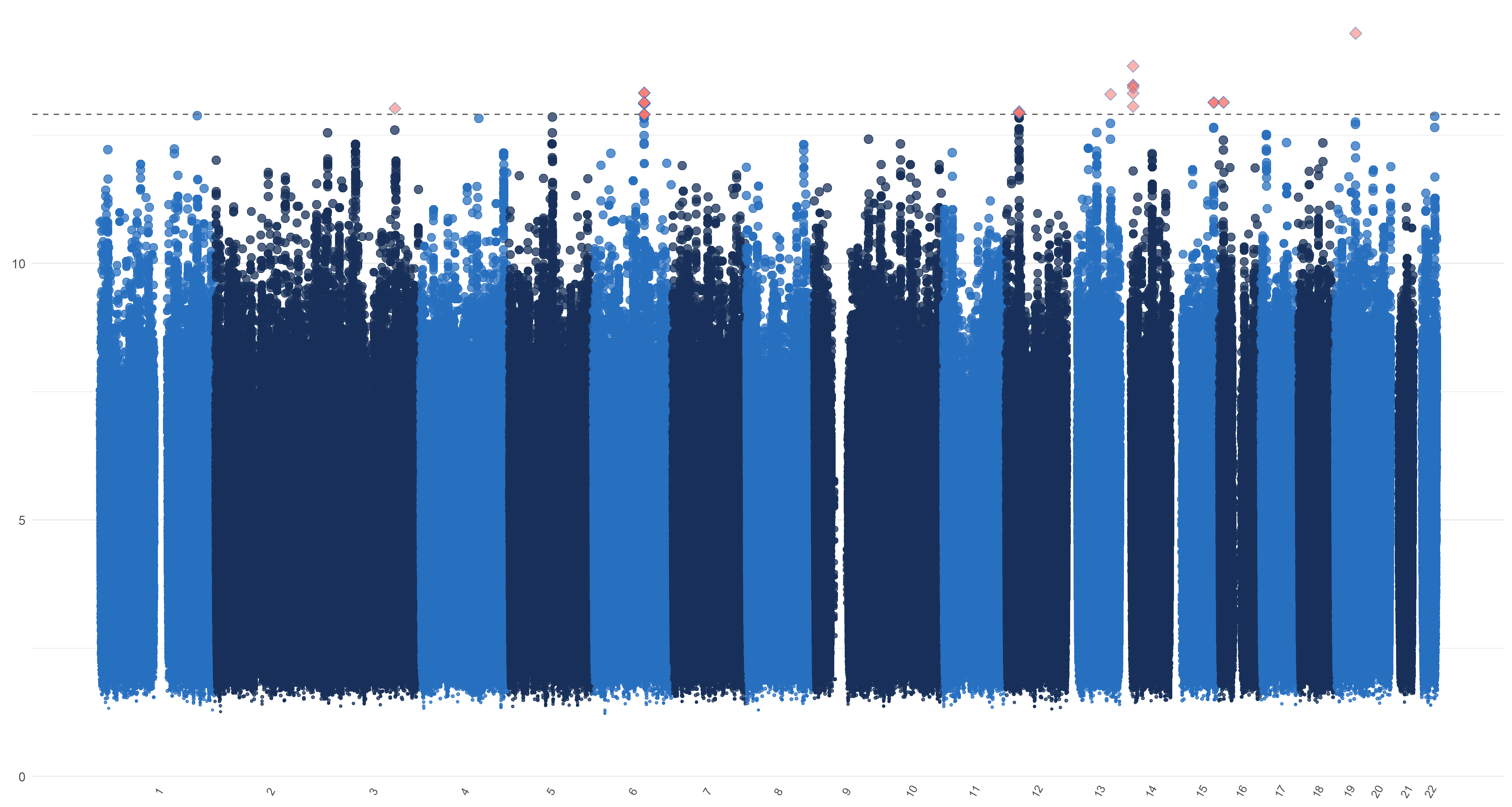
We use the default method (Gabriel et al., 2002) of Haploview (Barrett et al., 2005) and PLINK (Purcell et al., 2007) to form linkage disequilibrium (LD) blocks. Previous studies report that about 50 genetic variants are associated with AD; see the review in Sims et al. (2020) for details. This provides support for our assumption that (). On the other hand, a genome-wide association analysis of 19,629 individuals by Zhao et al. (2019) shows that genetic variants are associated with the left hippocampal volumes and are associated with the right hippocampal volumes. This provides support for our assumption that . Therefore, we apply our blockwise joint screening procedure on those SNPs on each part of hippocampal outcome and exposure marginally. We choose the thresholds , , and such that . In Table 3 of the supplementary material, we list the top SNPs corresponding to left and right hippocampi, respectively. As suggested by one referee, we plot similar figures as the Manhattan plot for , , and in Figure 7 of the supplementary material, where genomic coordinates are displayed along the x-axis, the y-axis represents the magnitude of , , and and the horizontal dashed line represents the threshold values , , , and , respectively.
From Table 3 and Figure 7, one can see that there are quite a few important SNPs for both hippocampi. For example, the top SNP is the rs429358 from the 19th chromosome. This SNP is a C/T single-nucleotide variant (snv) variation in the APOE gene. It is also one of the two SNPs that define the well-known APOE alleles, the major genetic risk factor for Alzheimer’s disease (Kim et al., 2009). In addition, a great portion of the SNPs in Table 3 has been found to be strongly associated with Alzheimer’s. These include rs10414043 (Du et al., 2018), an A/G snv variation in the APOC1 gene; rs7256200 (Takei et al., 2009), an A/G snv variation in the APOC1 gene; rs73052335 (Zhou et al., 2018), an A/C snv variation in the APOC1 gene; rs769449 (Chung et al., 2014), an A/G snv variation in the APOE gene; rs157594 (Hao et al., 2017), a G/T snv variation; rs56131196 (Gao et al., 2016), an A/G snv variation in the APOC1 gene; rs111789331 (Gao et al., 2016), an A/T snv variation; and rs4420638 (Coon et al., 2007), an A/G snv variation in the APOC1 gene.
Among those SNPs that have been found to be associated with Alzheimer’s, some of them are also directly associated with hippocampi. For example, Zhou et al. (2020) revealed that the SNPs rs10414043, rs73052335 and rs769449 are among the top SNPs that have significant genetic effects on the volumes of both left and right hippocampi. Guo et al. (2019) identified the SNP rs56131196 to be associated with hippocampal shape.
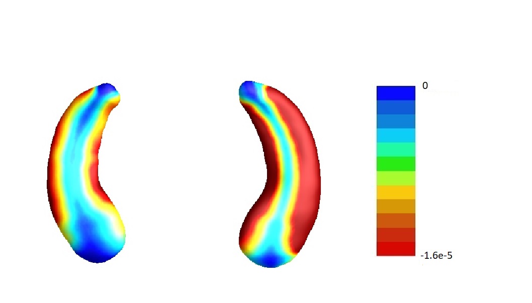
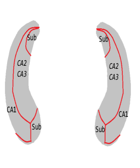
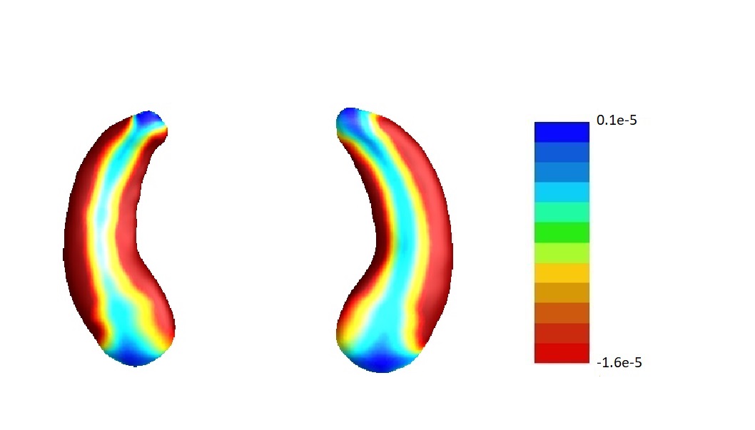
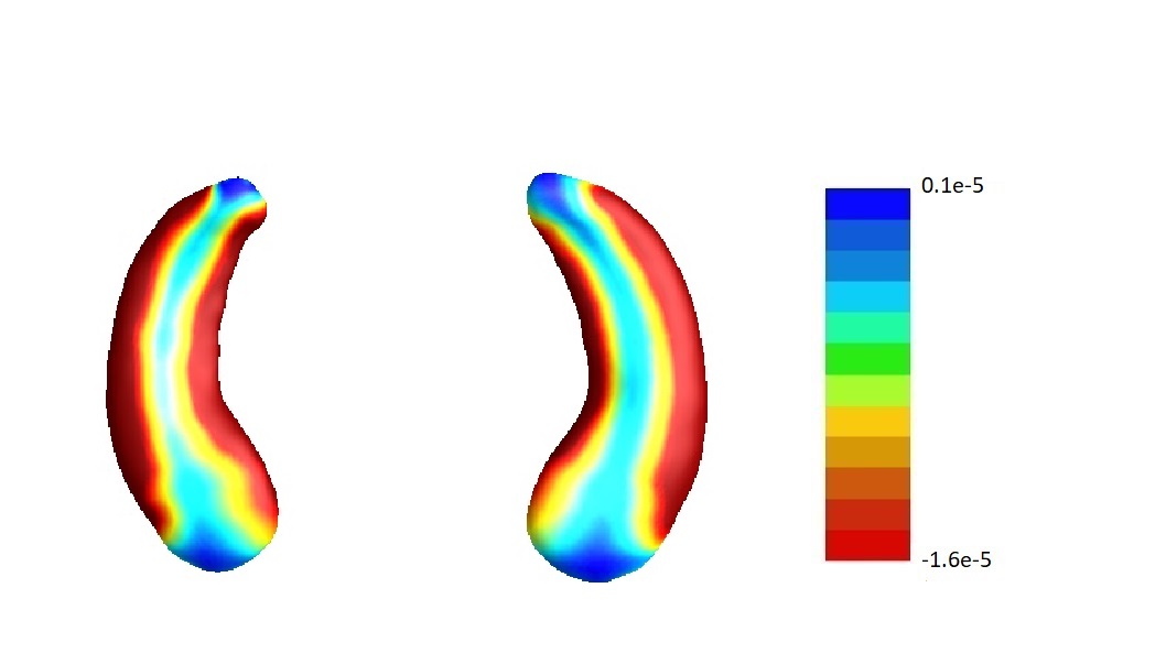
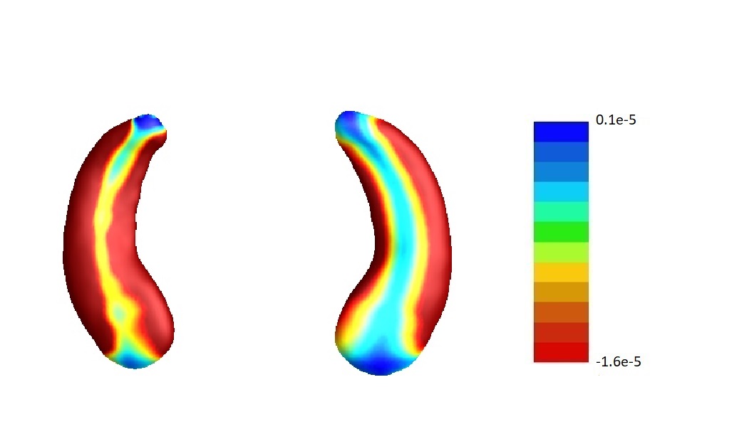
We then perform our second-step estimation procedure for each part of the hippocampi. Here denotes the SNPs selected in the screening step, the population stratification (top five principal components of the whole genome data) and the five clinical measures (age, gender, education length, baseline ICV and baseline diagnosis status), and denotes the left/right hippocampal surface image matrix. To visualize the results, we map the estimates corresponding to each part of the hippocampus onto a representative hippocampal surface and plot it in Figure 3(a). We have also plotted the hippocampal subfield (Apostolova et al., 2006) in Figure 3(b). Here Cornu Ammonis region 1 (CA1), Cornu Ammonis region 2 (CA2) and Cornu Ammonis region 3 (CA3) are a strip of pyramidal neurons within the hippocampus proper. CA1 is the top portion, named as “regio superior of Cajal” (Blackstad et al., 1970), which consists of small pyramidal neurons. Within the lower portion (regio inferior of Cajal), which consists of larger pyramidal neurons, there are a smaller area called CA2 and a larger area called CA3. The cytoarchitecture and connectivity of CA2 and CA3 are different. The subiculum is a pivotal structure of the hippocampal formation, positioned between the entorhinal cortex and the CA1 subfield of the hippocampus proper (for a complete review, see Dudek et al. 2016).
From the plots, we can see that all the entries of corresponding to both hippocampi are negative. This implies that the radial distance of each pixel of both hippocampi is negatively associated with the ADAS-13 score, which depicts the severity of behavioral deficits. The subfields with strongest associations are mostly CA1 and subiculum. Existing literature (Apostolova et al., 2010) has found that as Alzheimer’s disease progresses, it first affects CA1 and subiculum subregions and later CA2 and CA3 subregions. This can partially explain why the shapes of CA1 and subiculum may have stronger associations with ADAS-13 scores compared to CA2 and CA3 subregions.
We examine the effect size of the whole hippocampal shape by evaluating the term . Specifically, we calculate the proportion of variance explained by imaging covariates as follows:
Our results show that the shape of the left hippocampi and that of the right one account for 5.83% and 4.71% of the total variations in behavior deficits, respectively. Such effect sizes are quite large compared with those for polygenic risk scores in genetics. In addition, we perform permutation test to test whether the statistic is significant. In particular, we randomly permutate the , denoted by , and we then apply our estimation procedure based on , obtain , and calculate . We repeat this for 1,000 times and and we obtain the , which mimics the null distribution. Finally, the p-value can be calculated as . The p-values for both hippocampi are less than , suggesting that the ’s are significantly different from zero.
We also conduct sensitivity analysis by varying the relative sizes of and in the joint screening procedure. The estimates s are similar among different choices of and ; see supplementary material Section 11 for details. In addition, we repeated our analysis on the MCI and AD subjects. We have similar findings that the radial distances of each pixel of both hippocampi are mostly negatively associated with the ADAS-13 score. And the subfields with strongest associations are mostly CA1 and subiculum; see supplementary material Section 12 for details. As suggested by one referee, we have performed the SNP-imaging-outcome mediation analysis proposed by Bi et al. (2017); see Section 13 in the supplementary material for the detailed procedure. There is no evidence for the mediating relationship of SNP-imaging-outcome from our analysis.
5 Simulation studies
In this section, we perform simulation studies to evaluate the finite sample performance of the proposed method. The dimension of covariates is set as , and the exposure is a matrix. The is independently generated from , where has an autoregressive structure such that holds for with . Define as a image shown in Figure 4(a), and a image shown in Figure 4(b). For , the black regions of interest (ROIs) are assigned value and white ROIs are assigned value . For , the black ROIs are assigned value and white ROIs are assigned value . Further we set , where , , , , , , and for and . We set the parameters , , , , , , and for and . In this setting, we have , , and .
The random error is independently generated from , where we set the standard deviations of all elements in to be and the correlation between and to be for with . The random error is generated independently from , where we consider or . The ’s and ’s are generated from models (1) and (2). We consider three different sample sizes and .
5.1 Simulation for screening
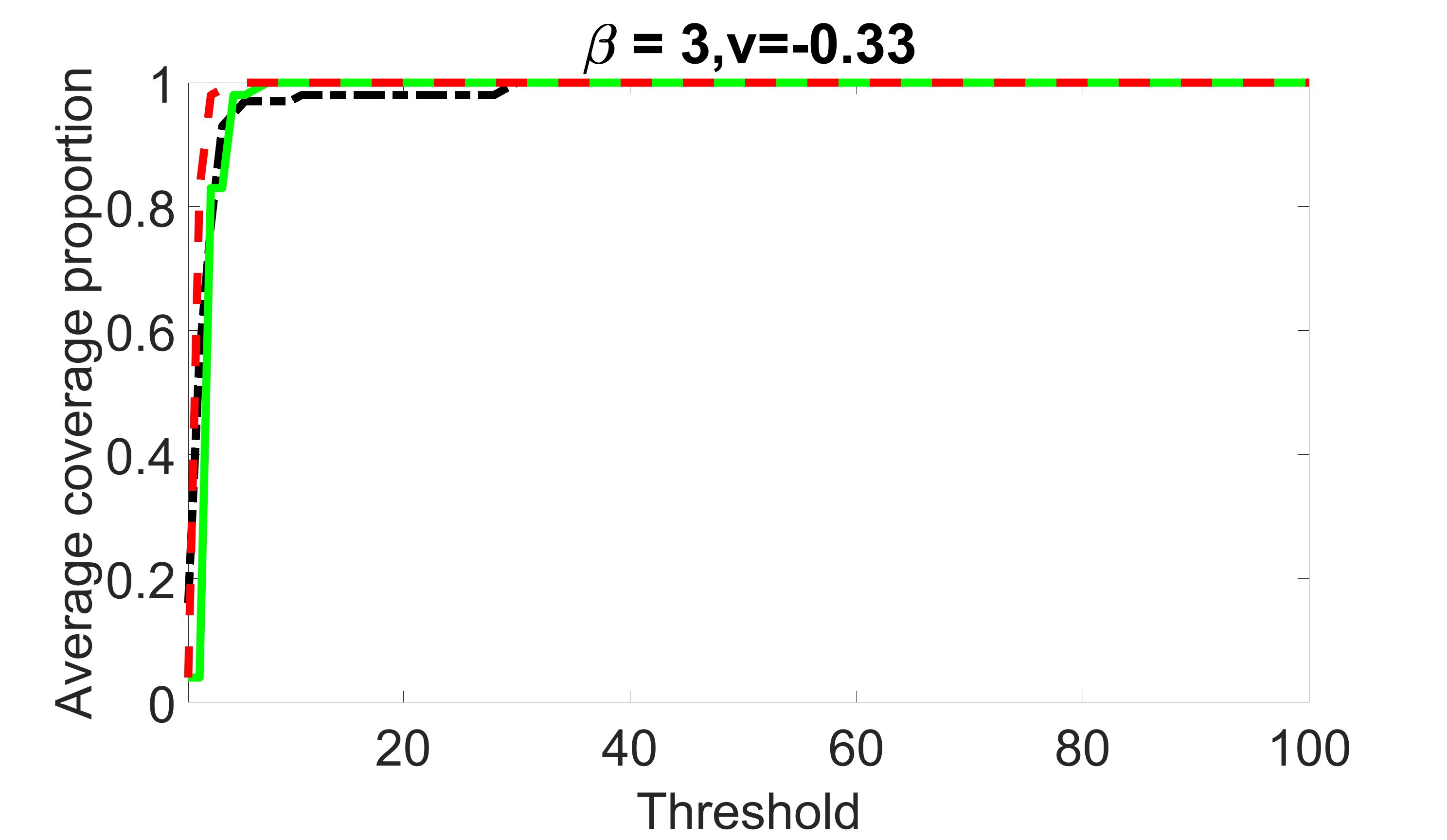
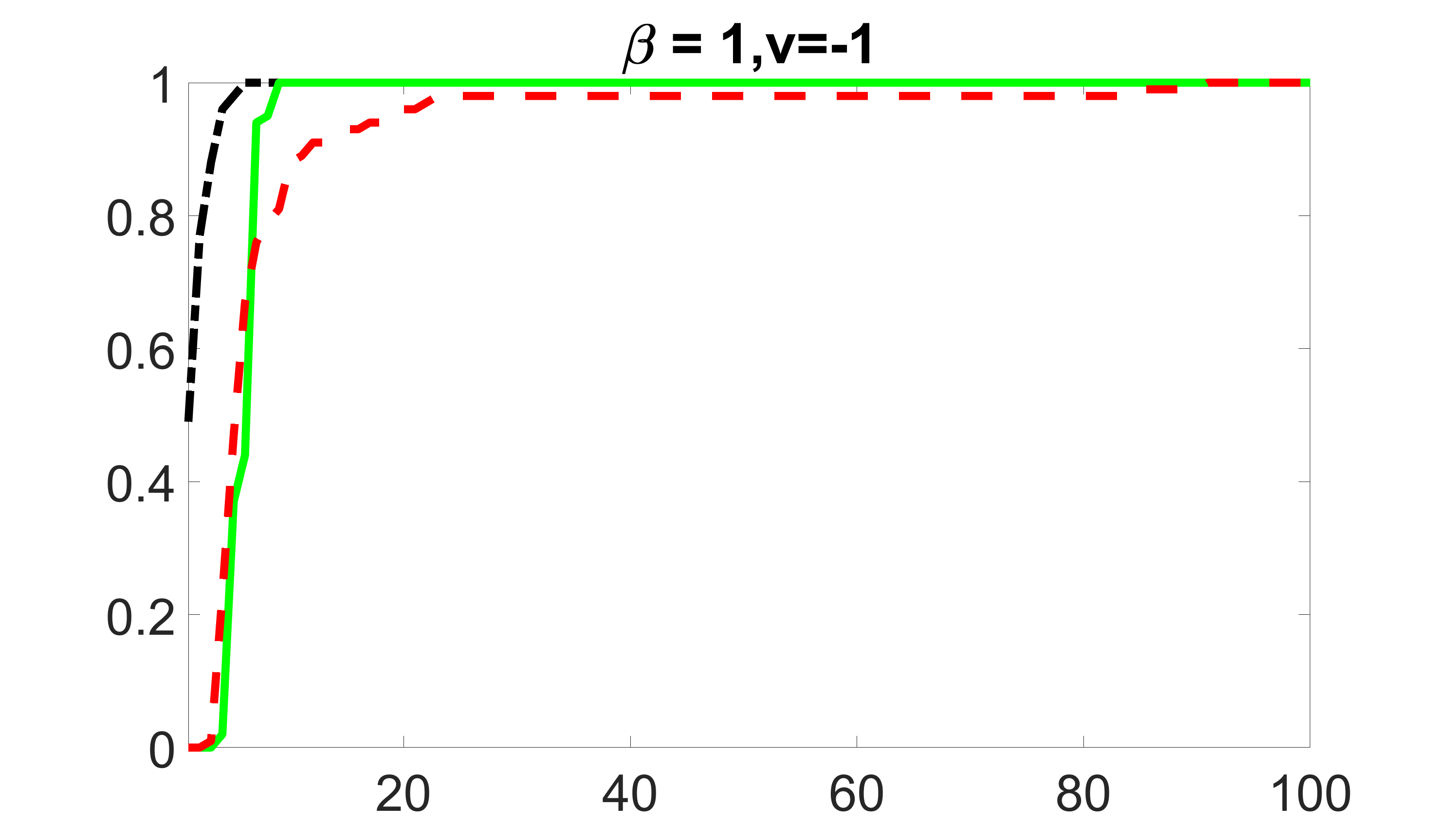
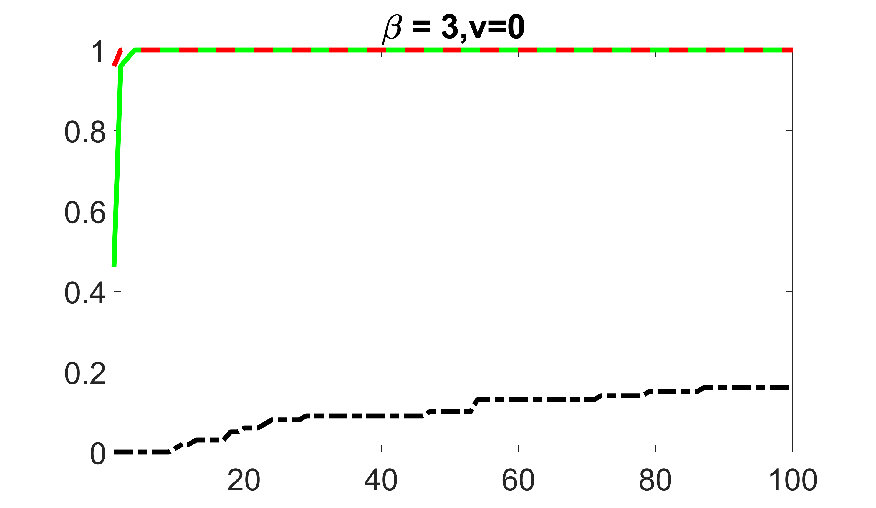
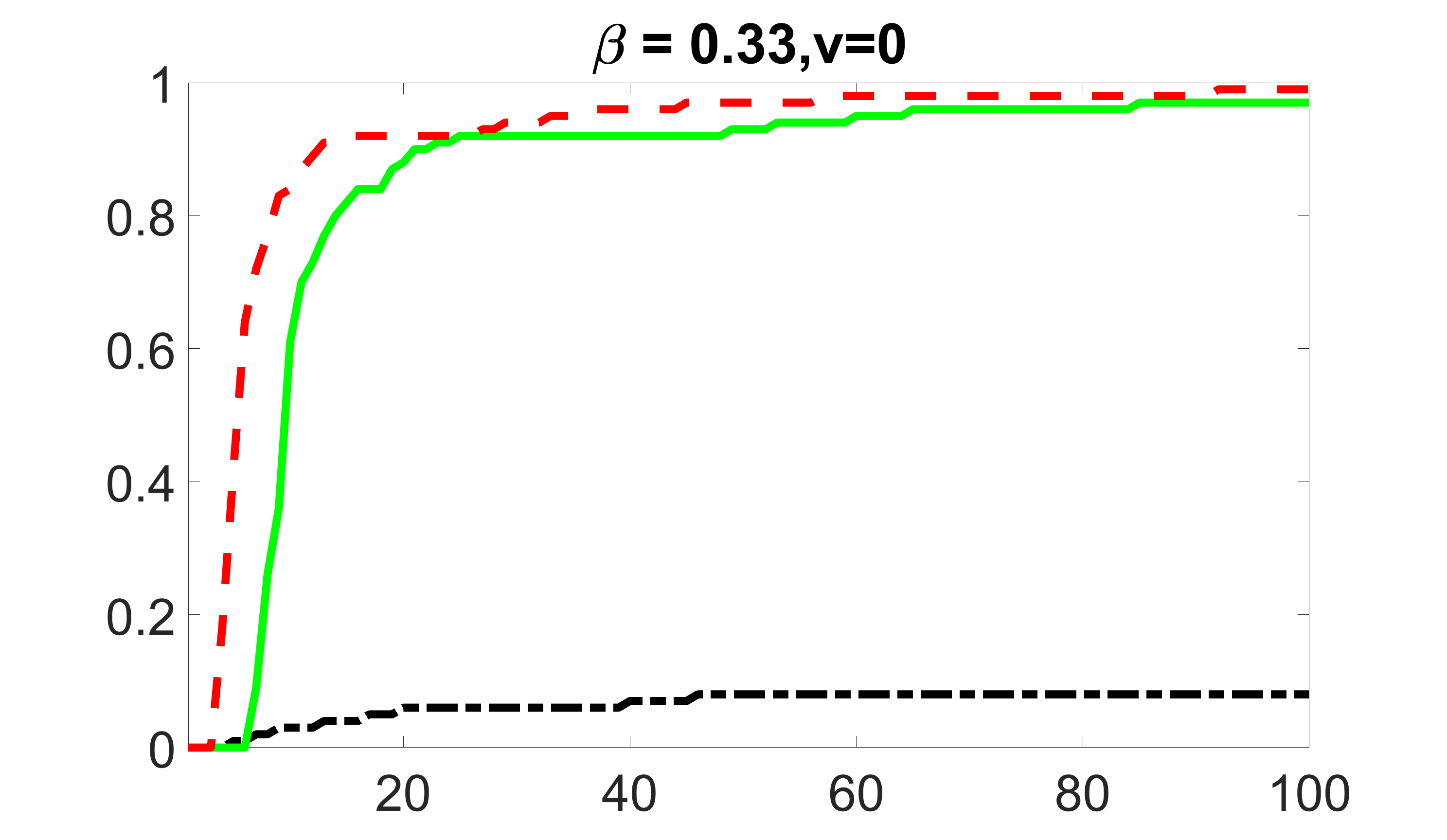
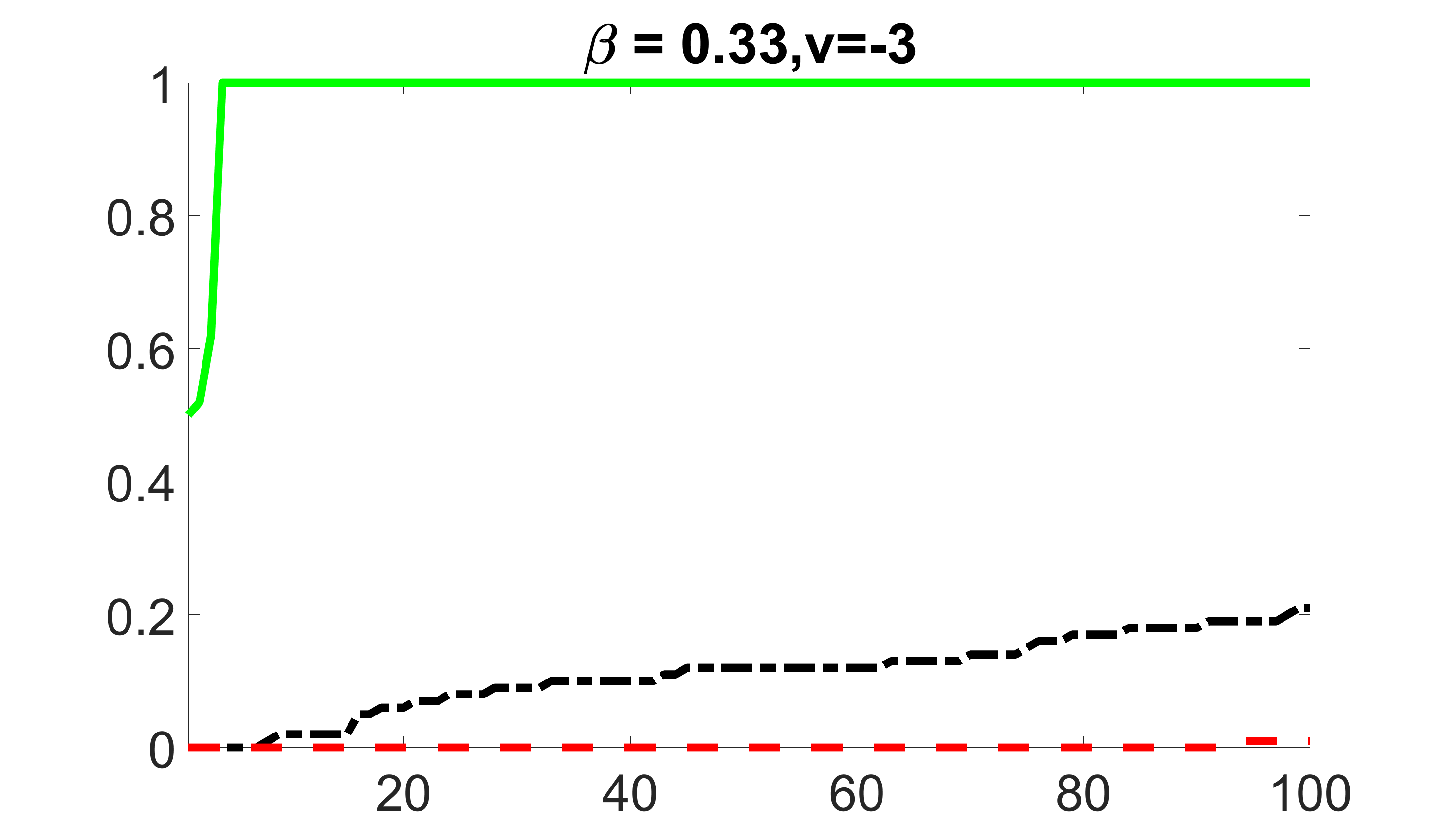
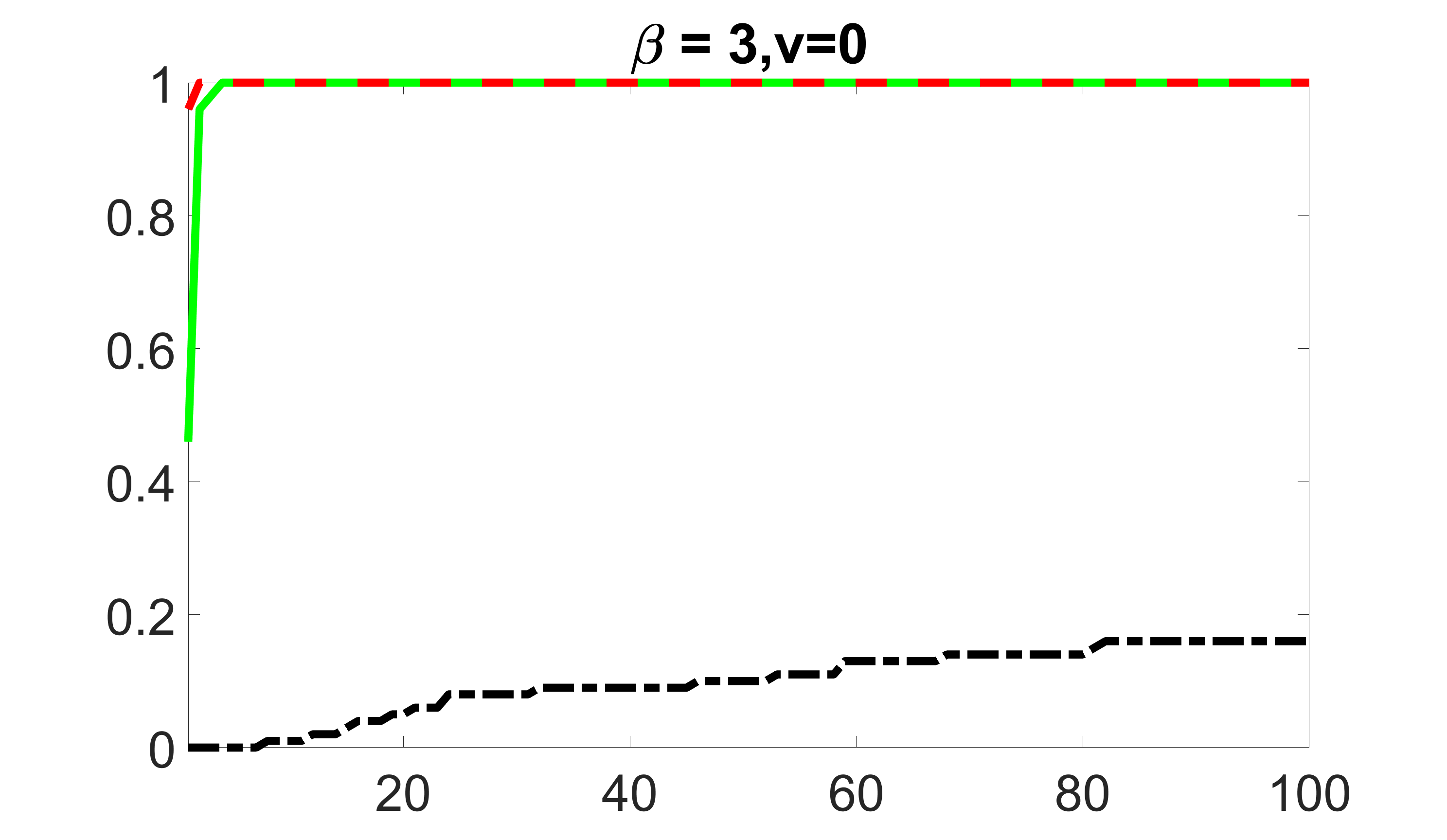
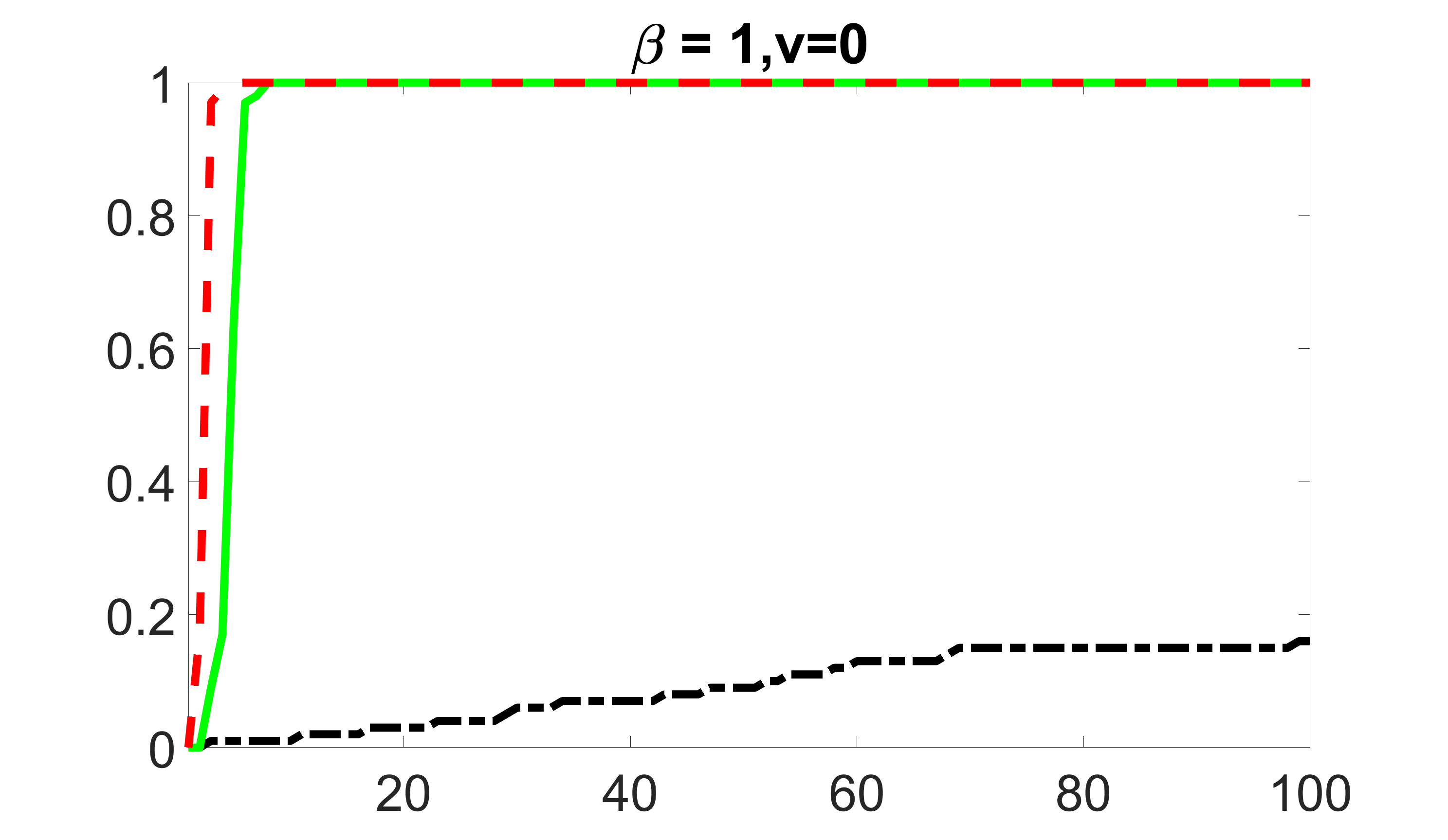
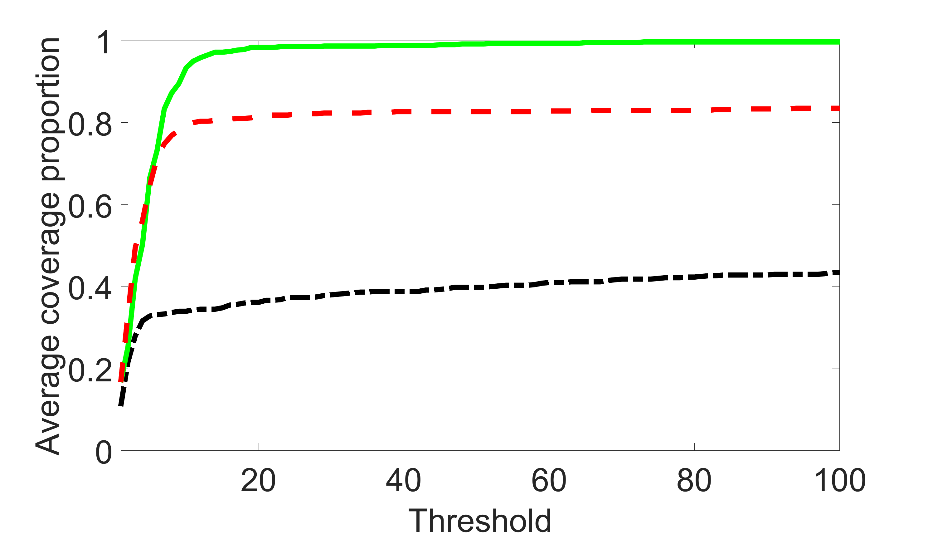
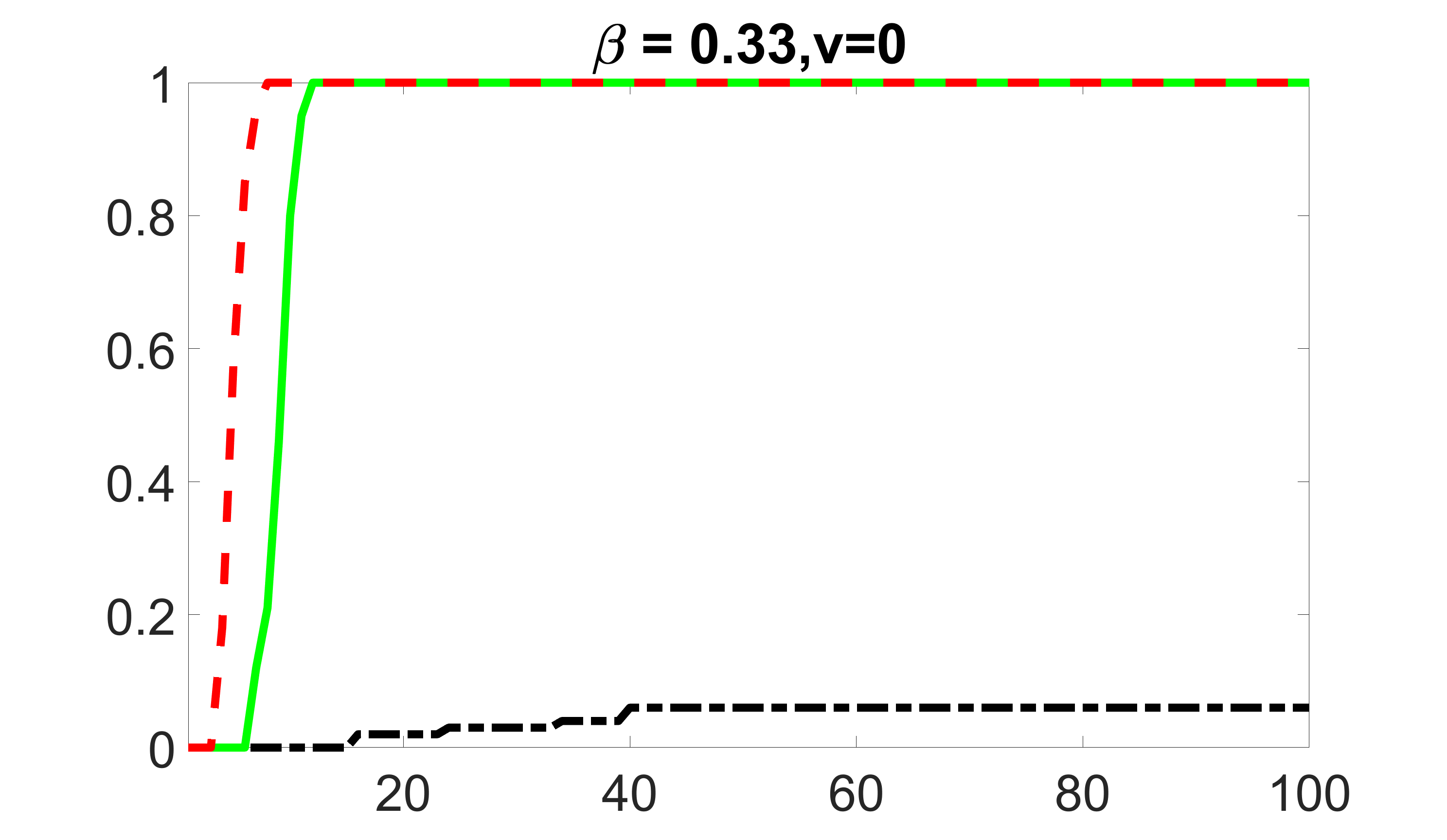
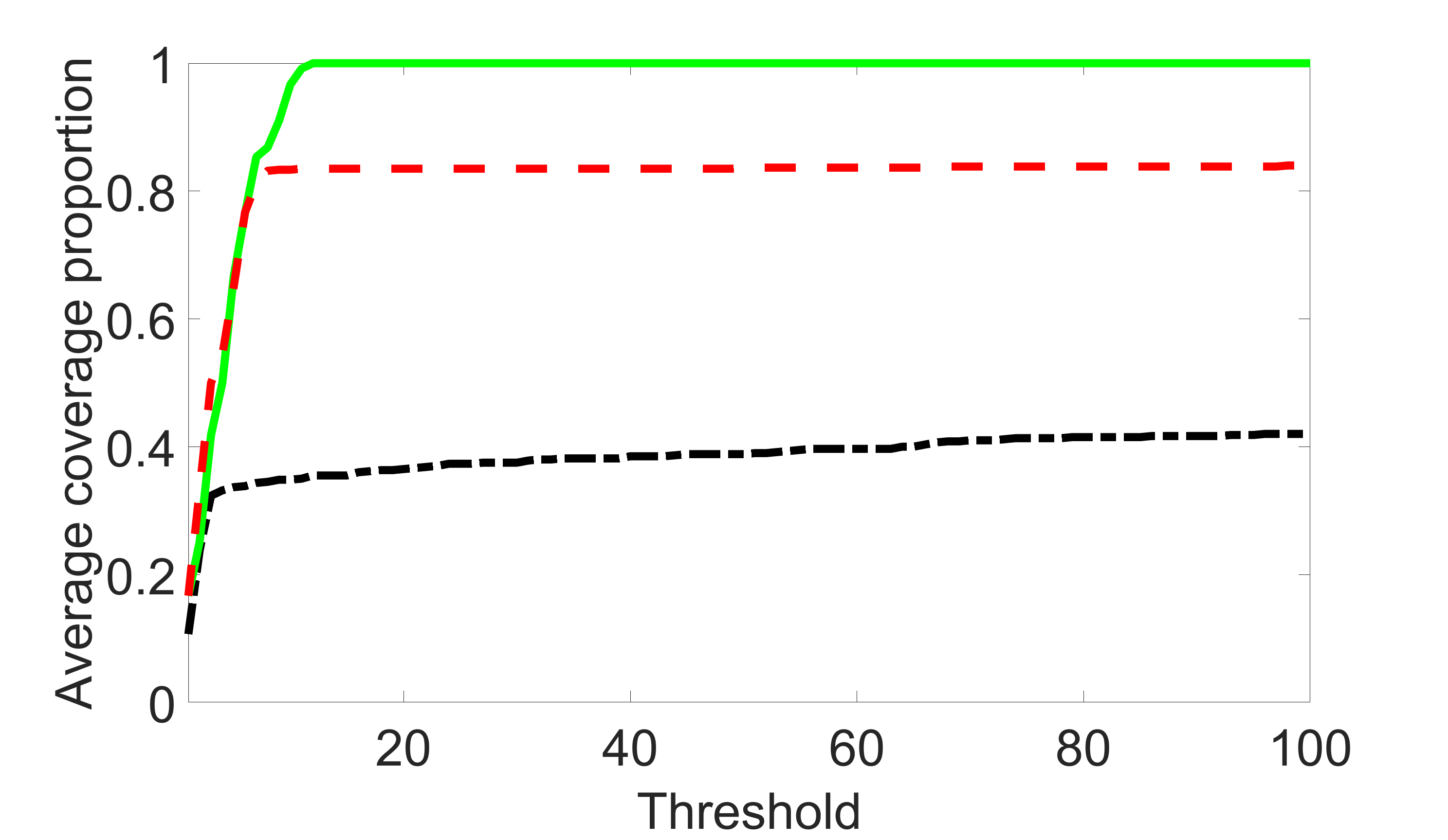
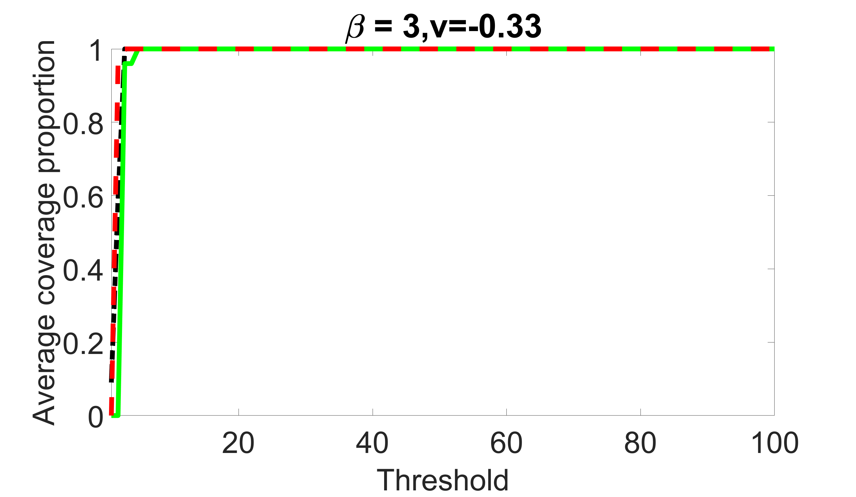
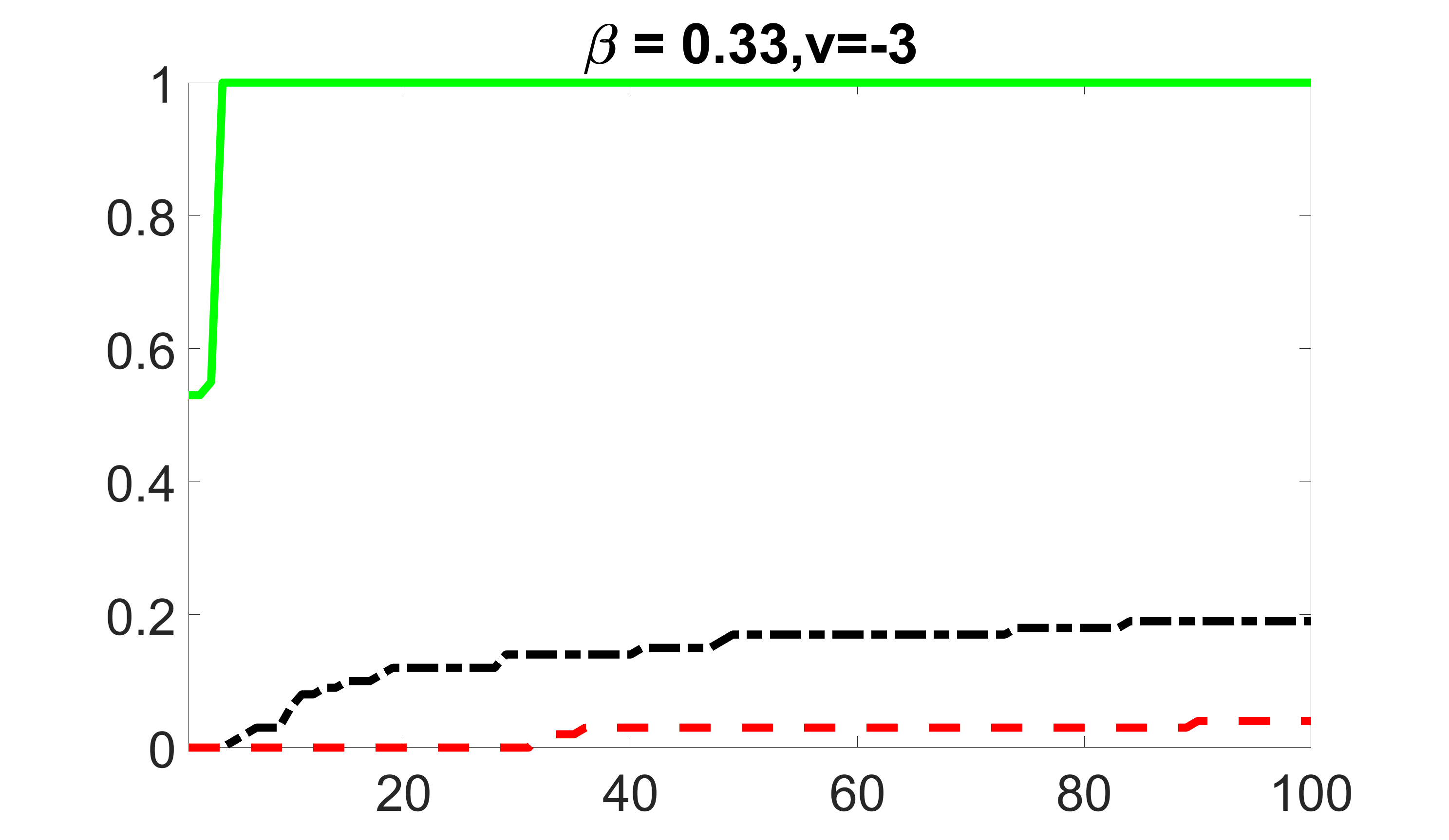
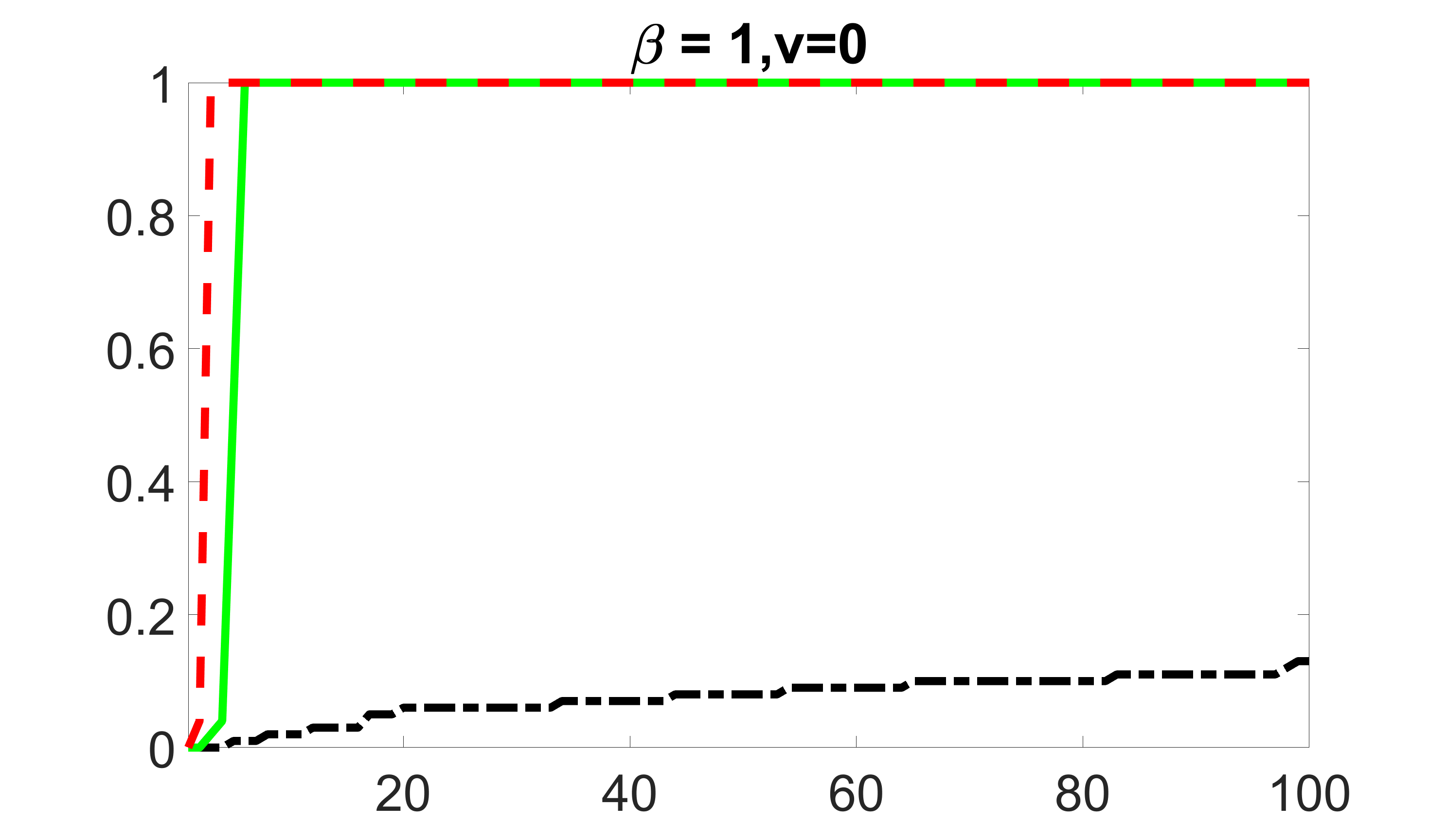
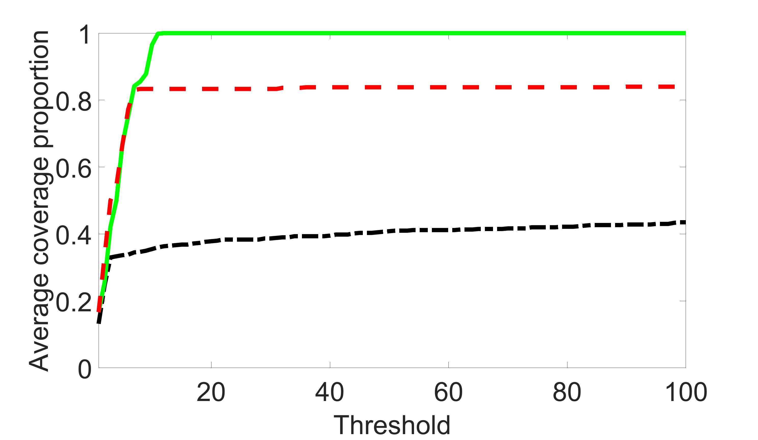
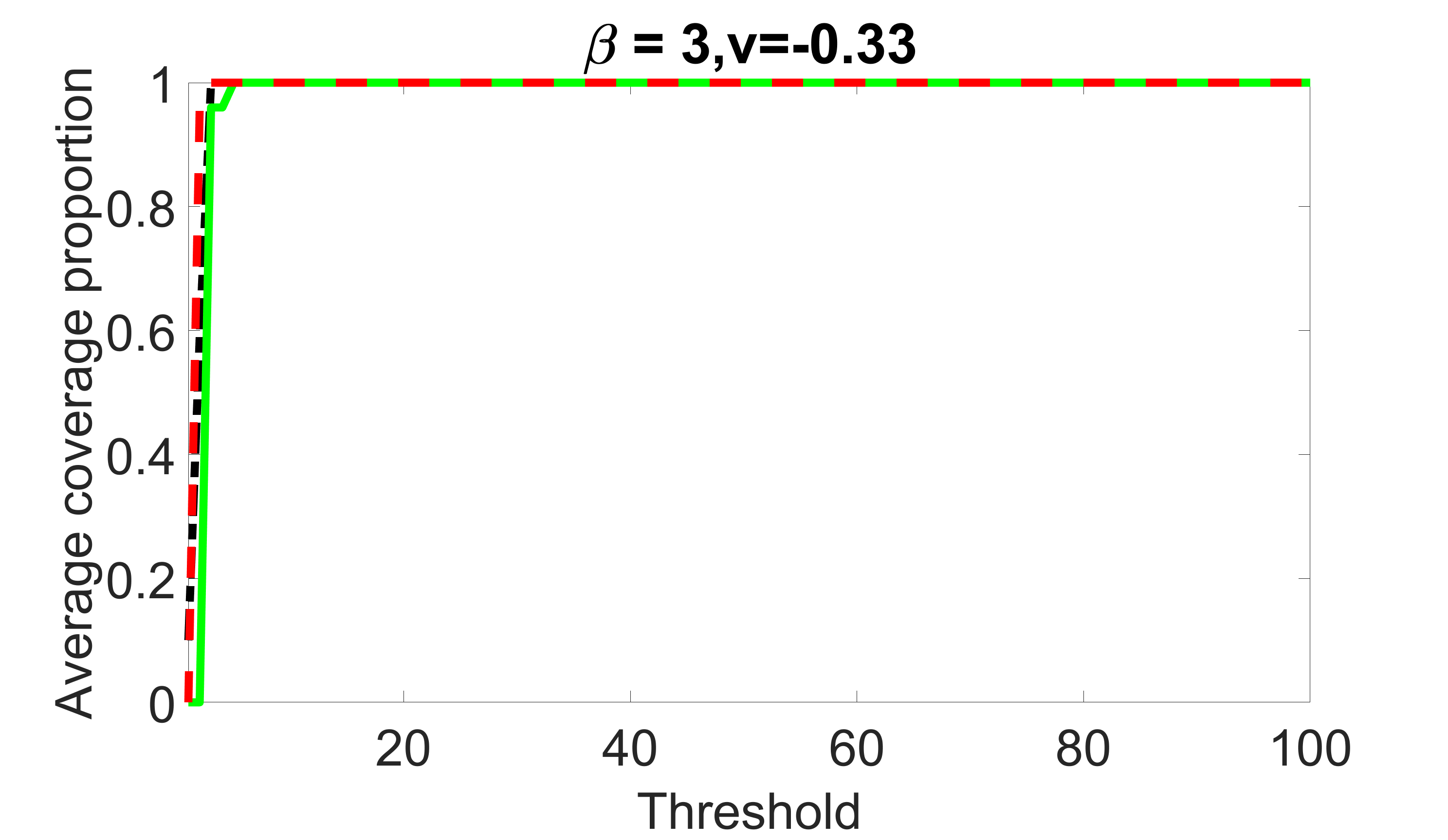
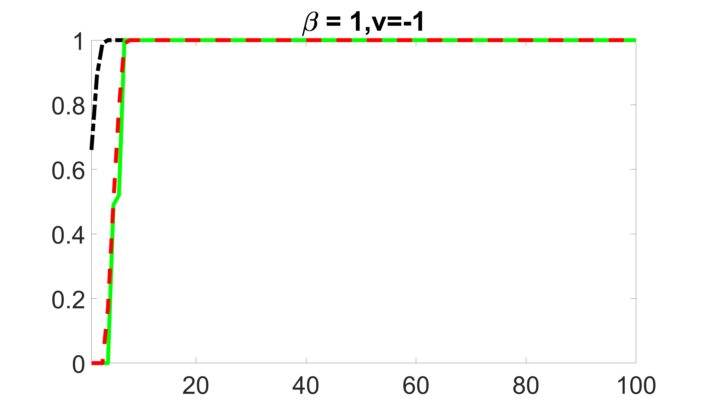
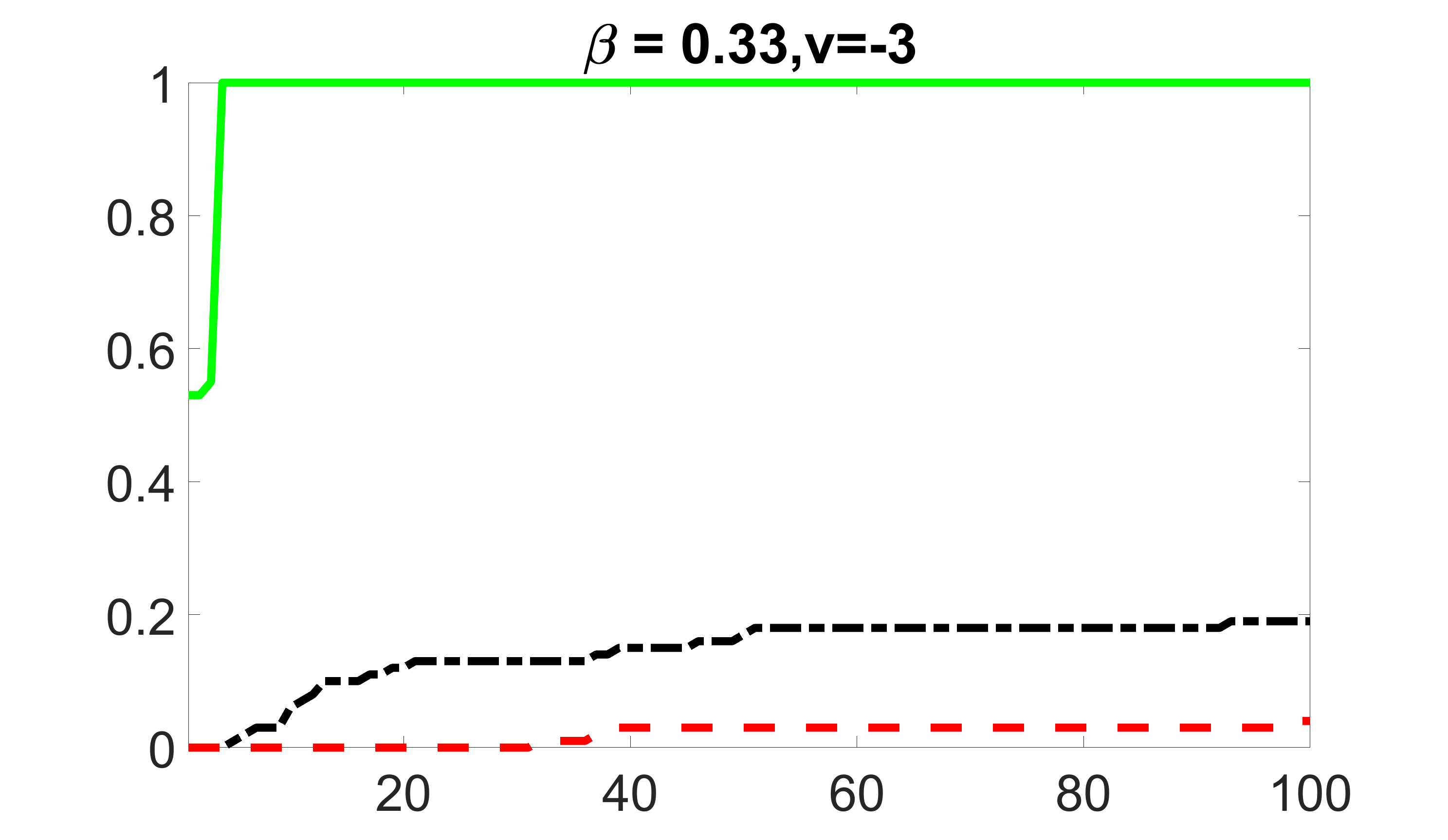
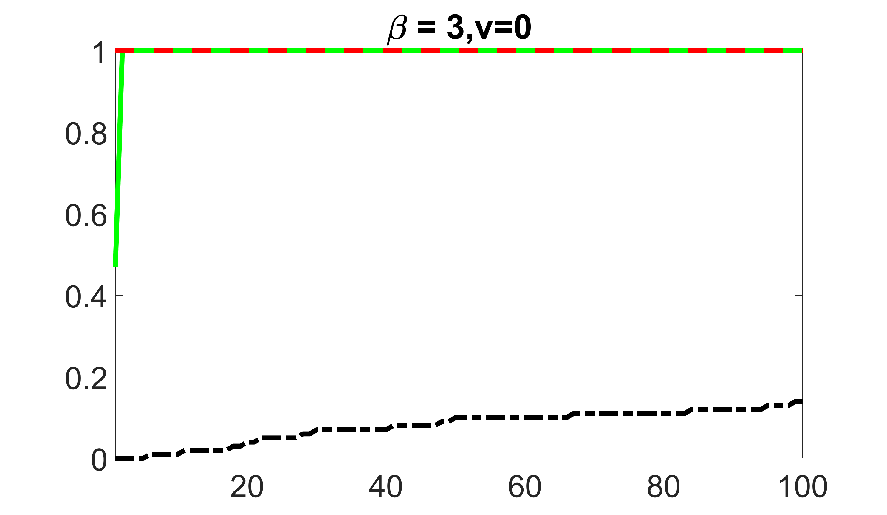
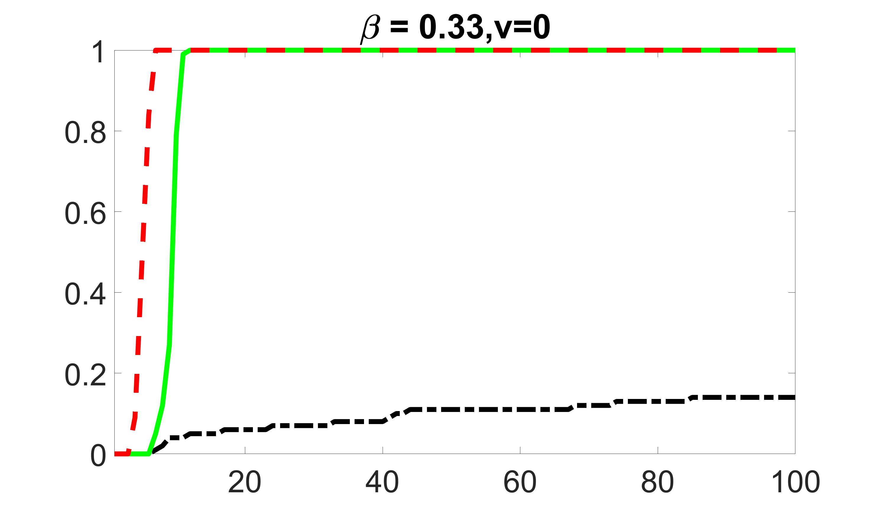
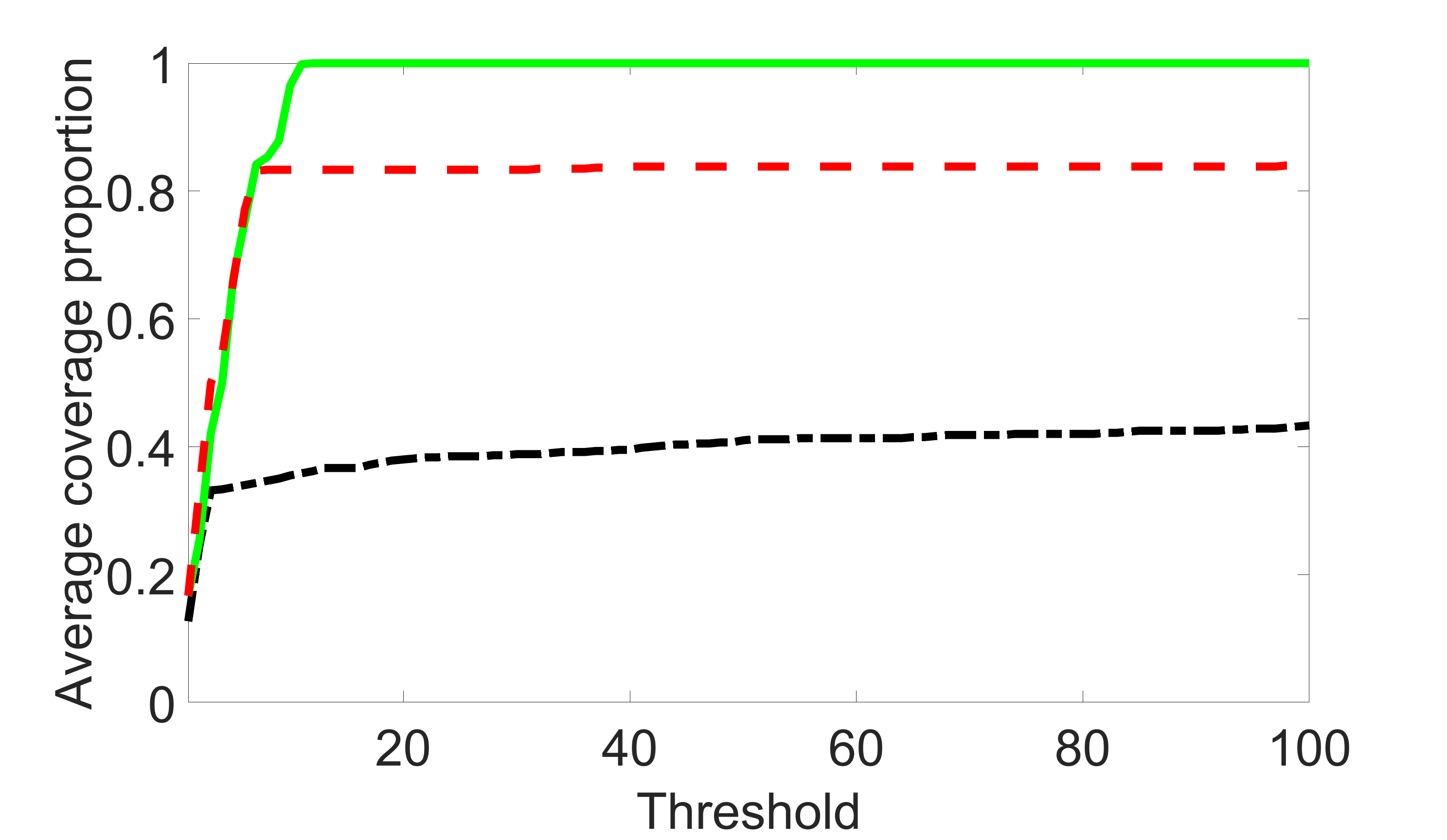
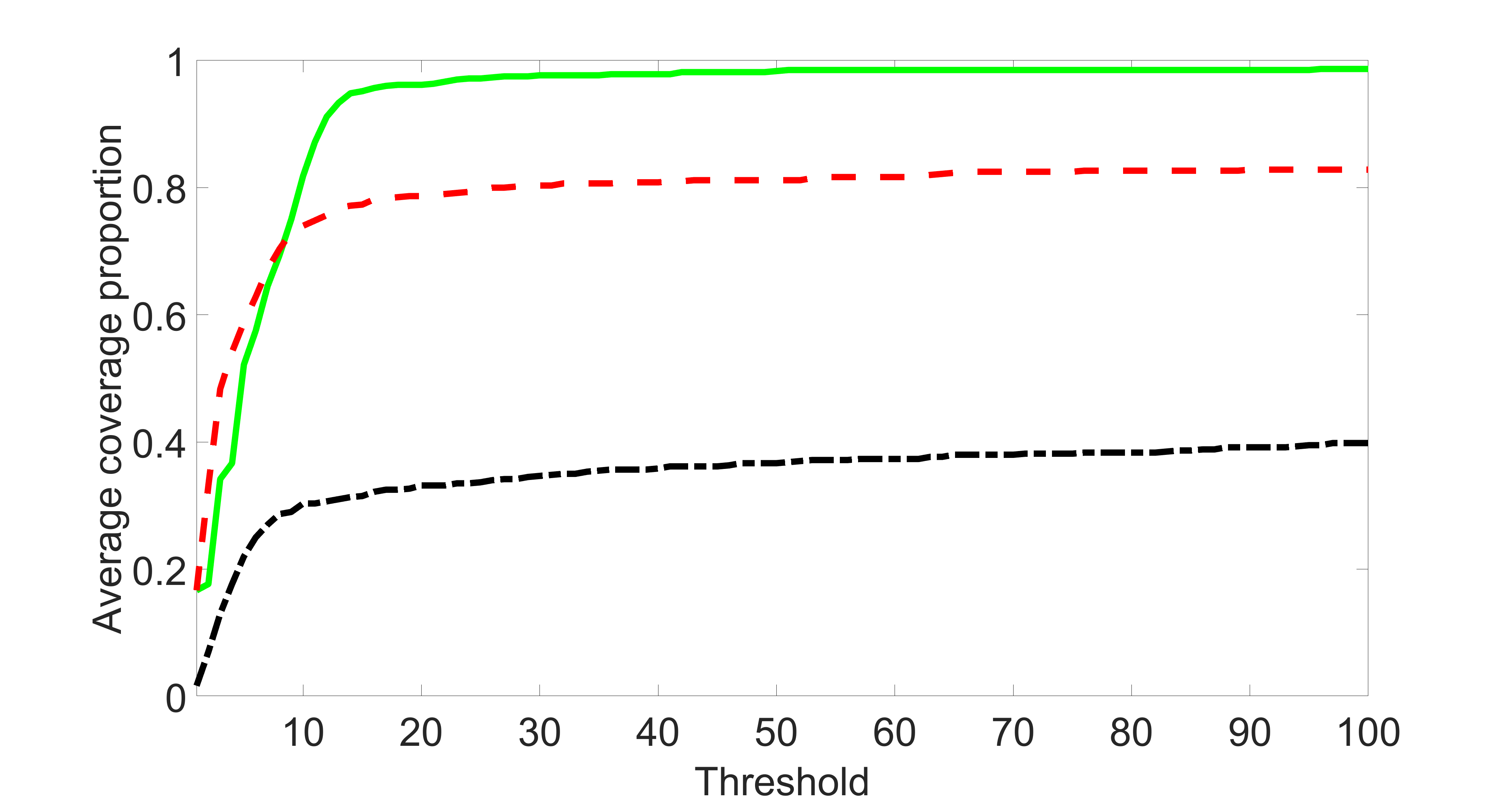
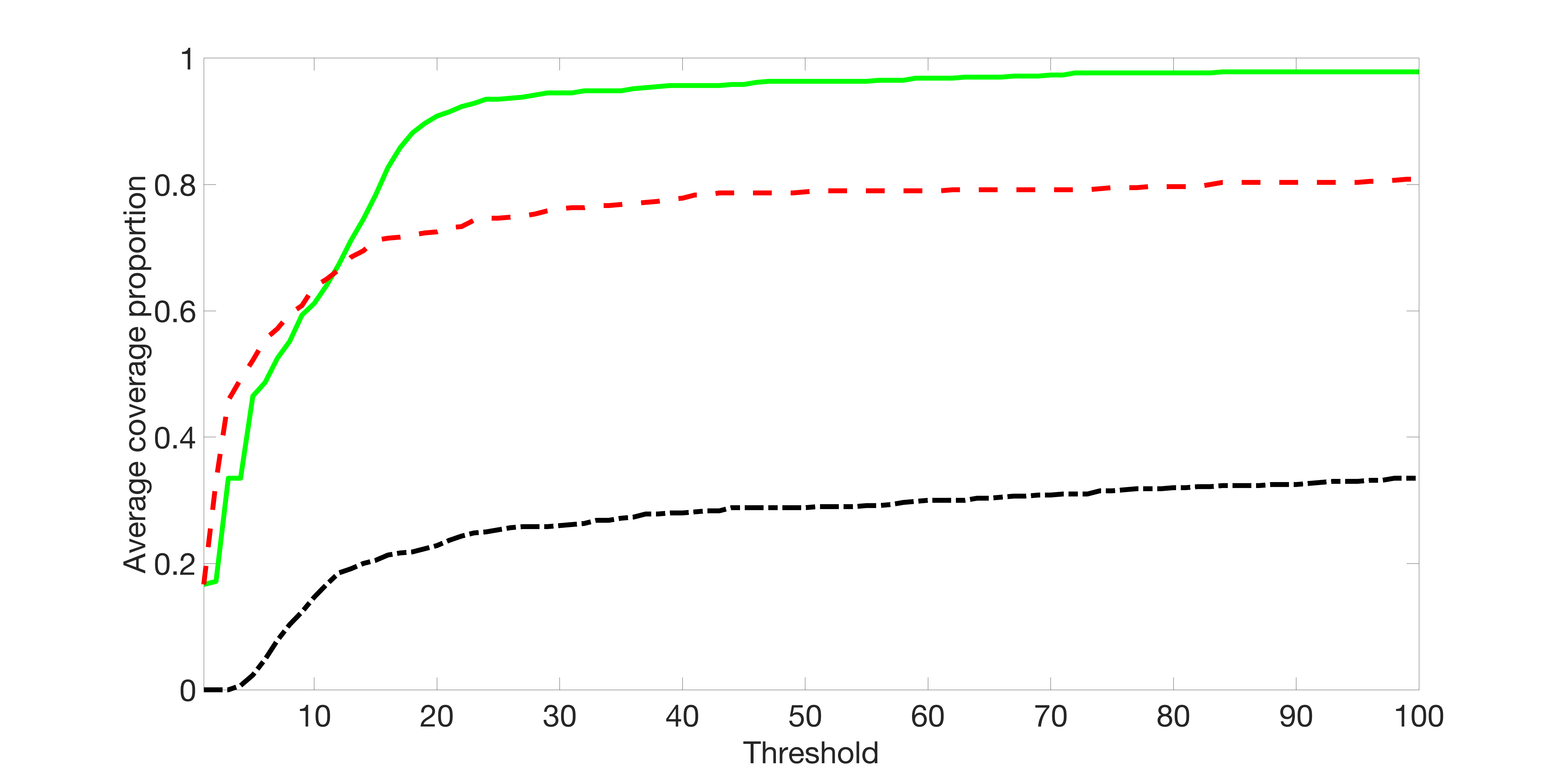
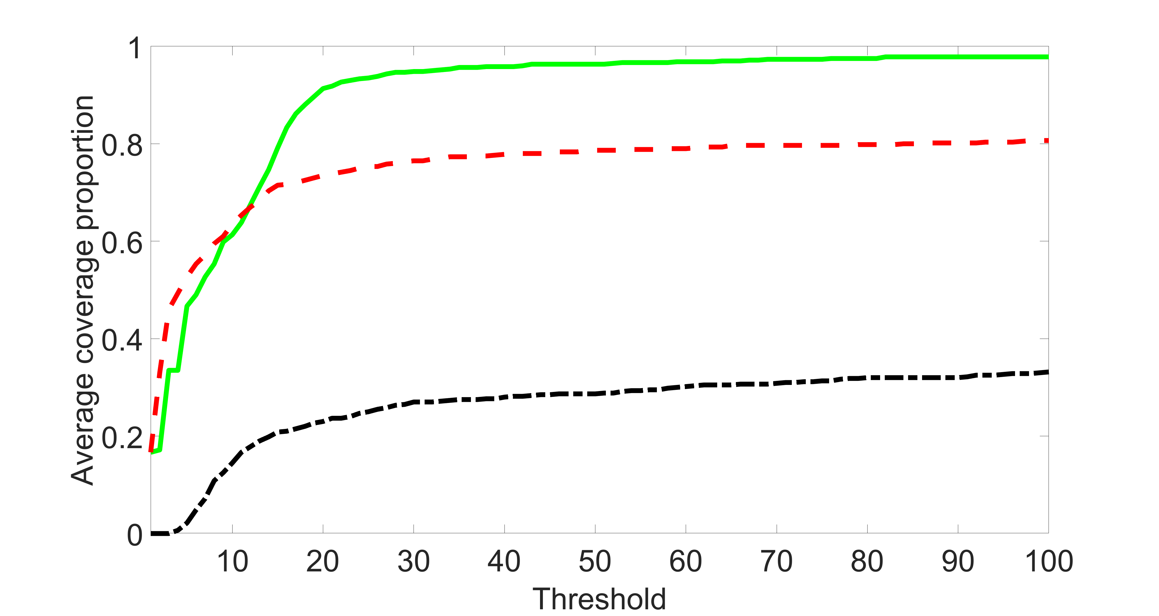
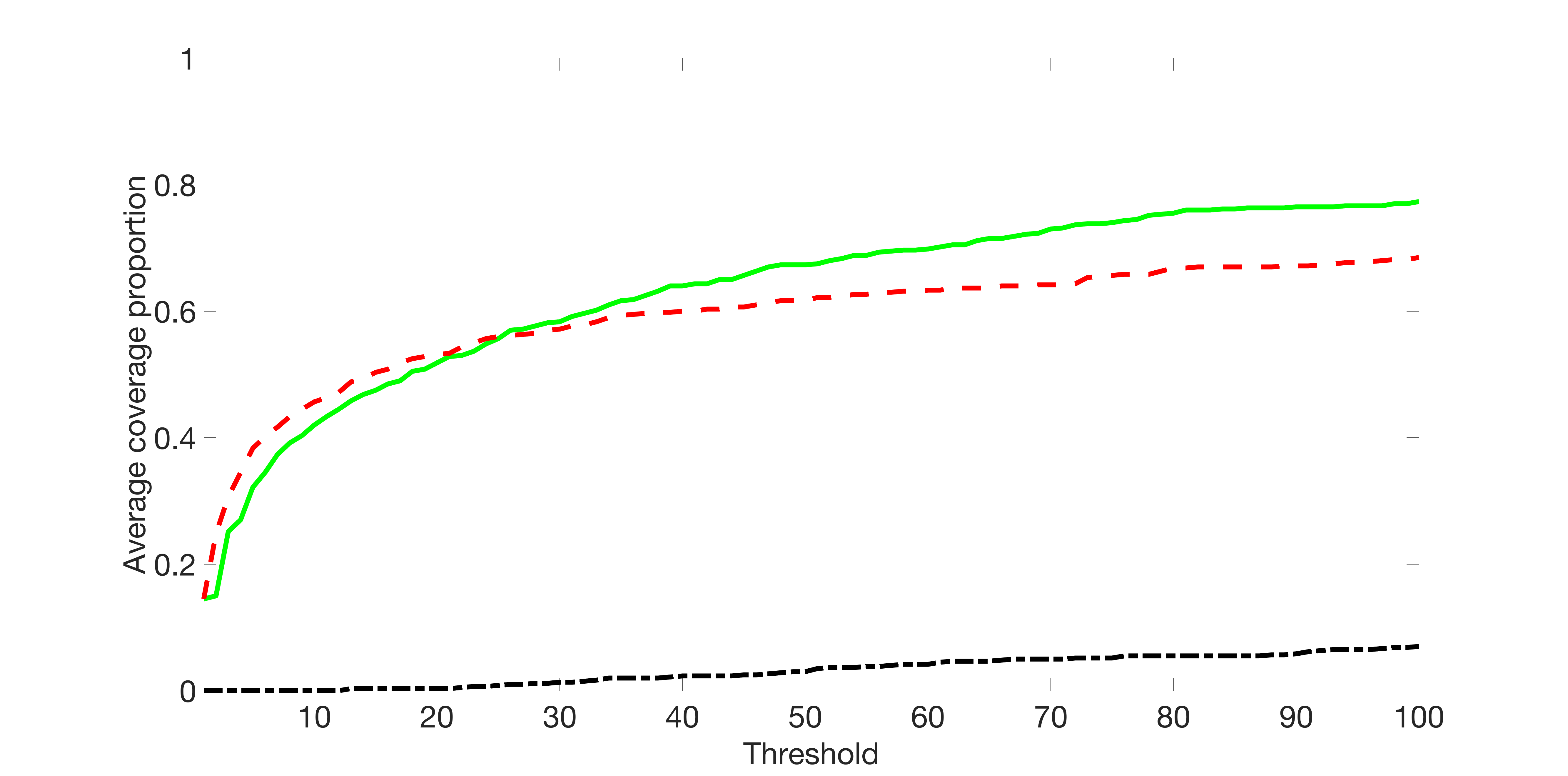
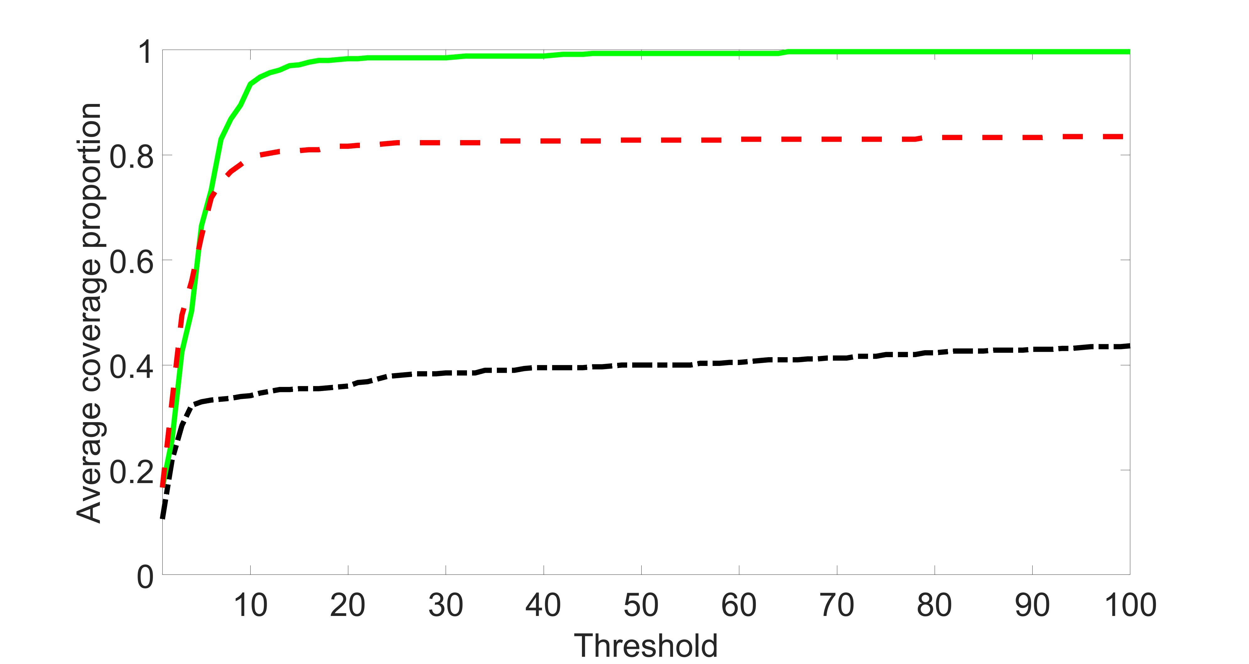
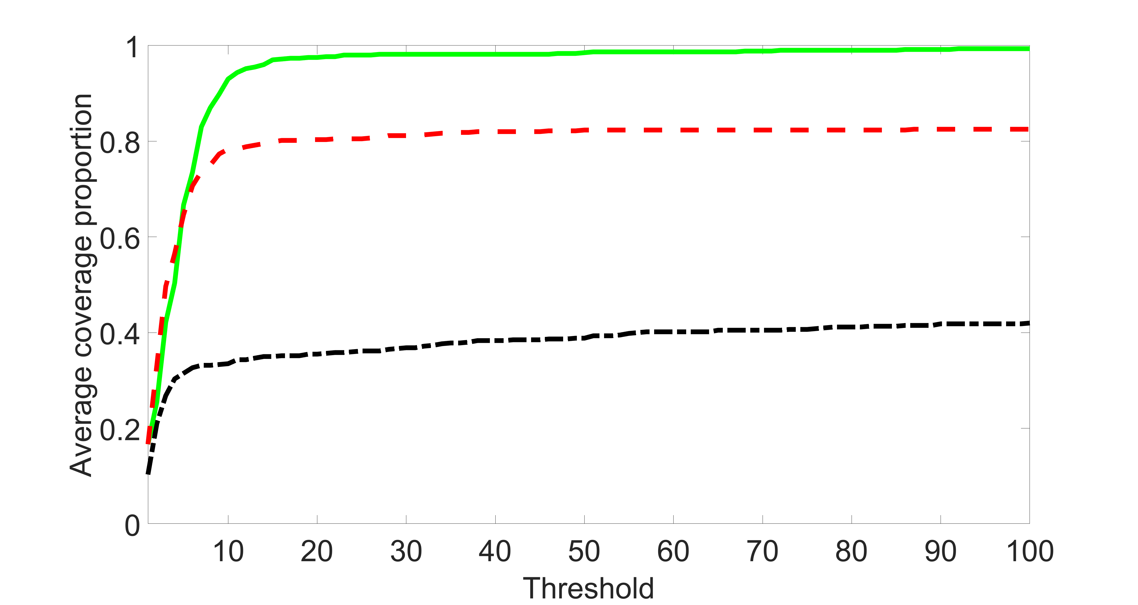
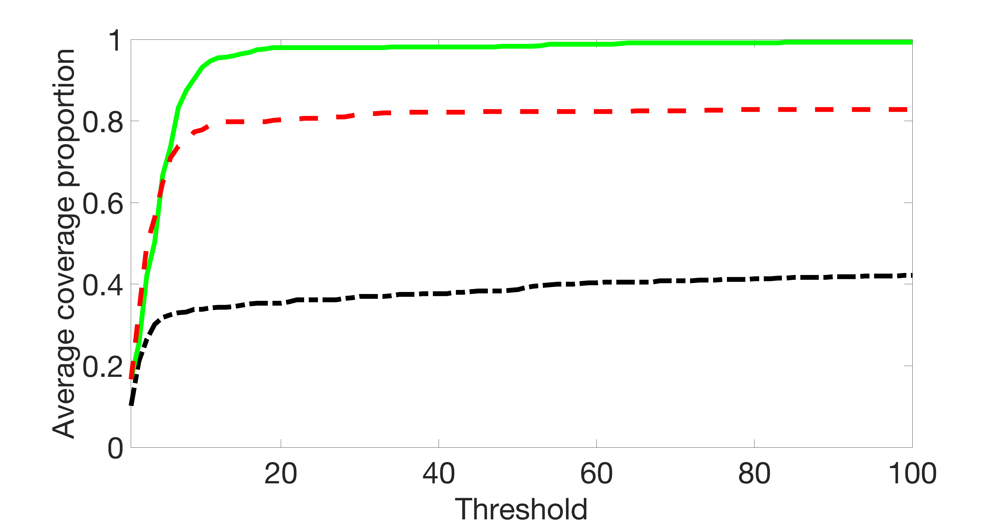
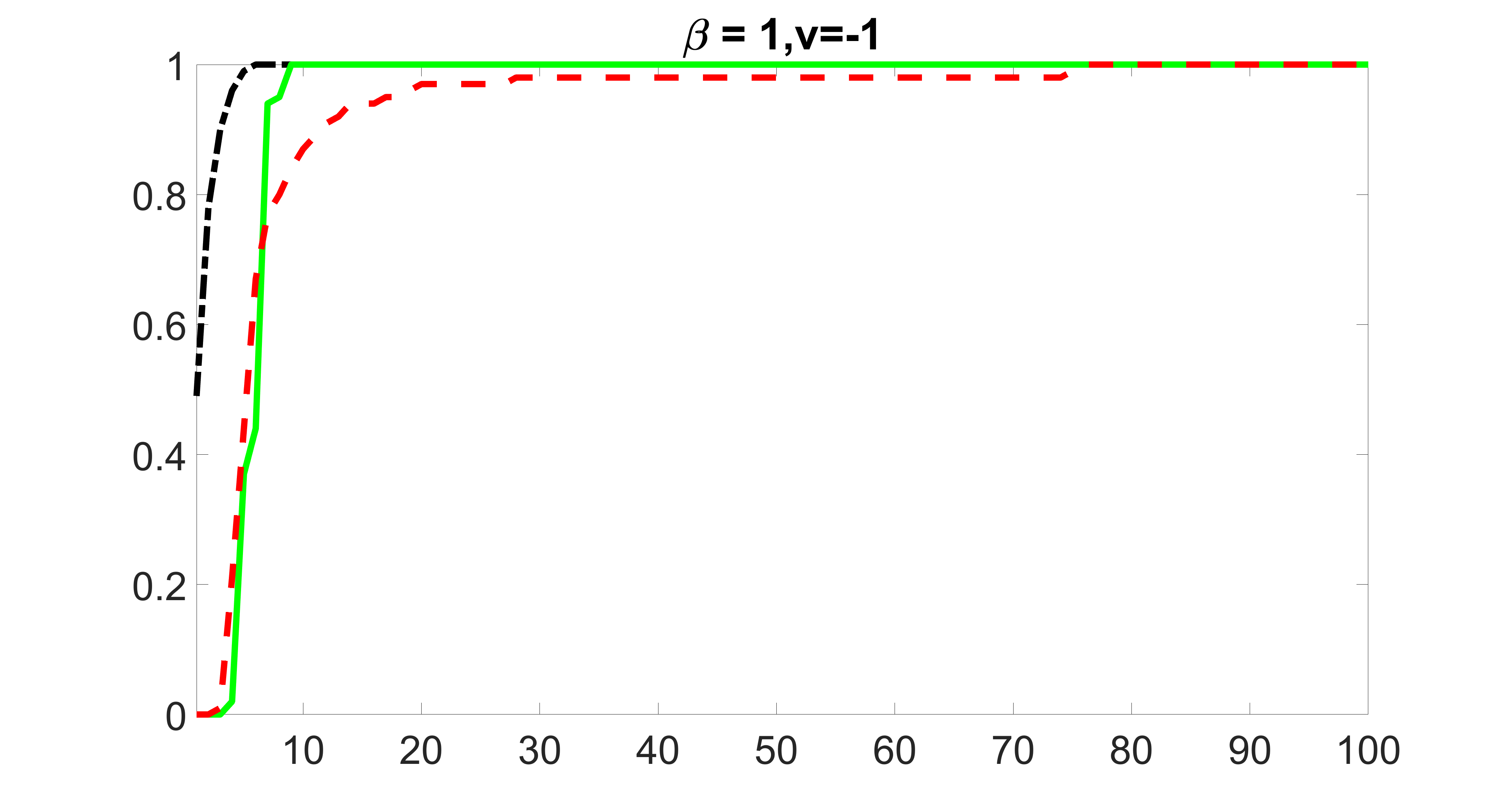
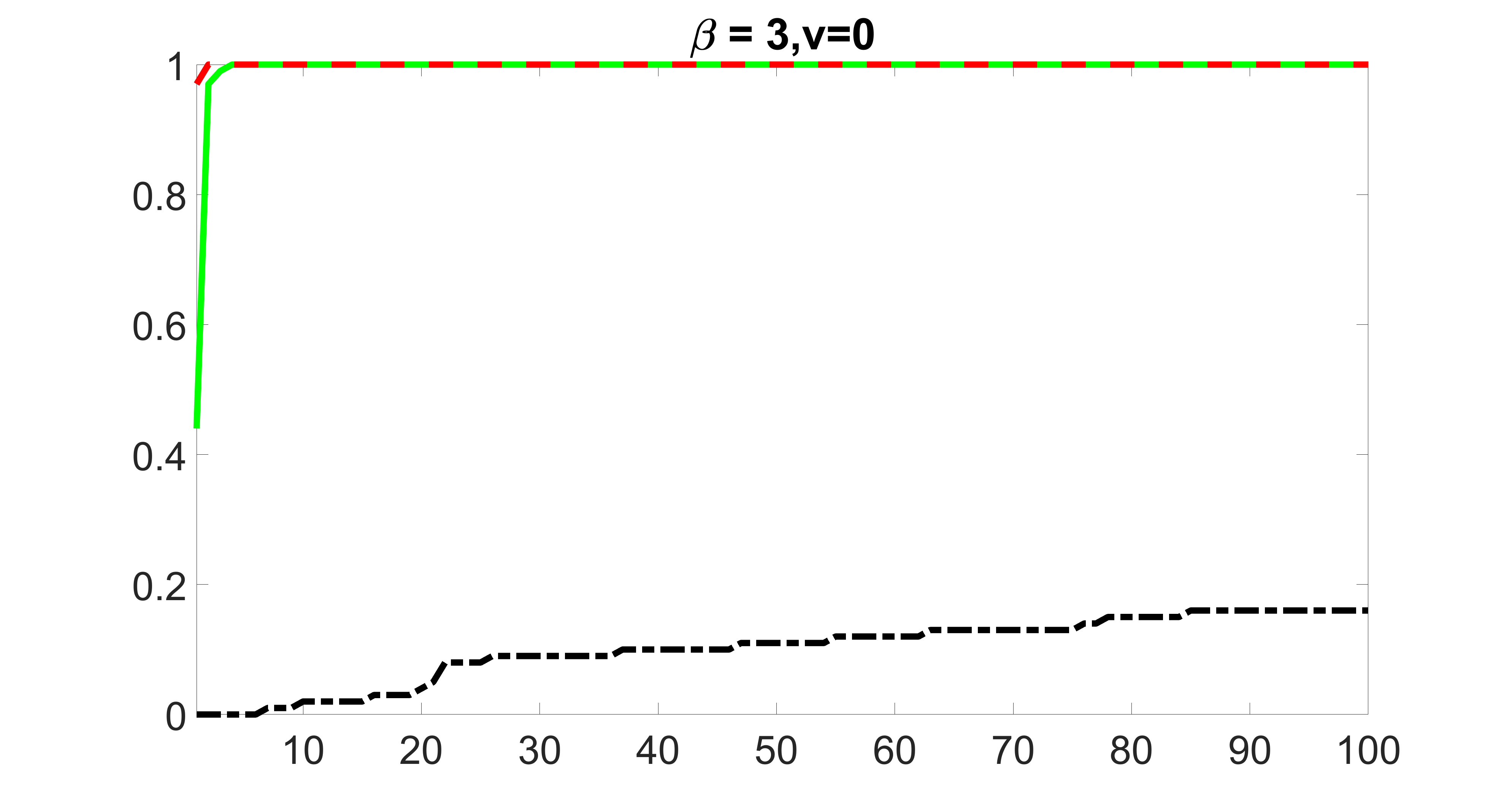
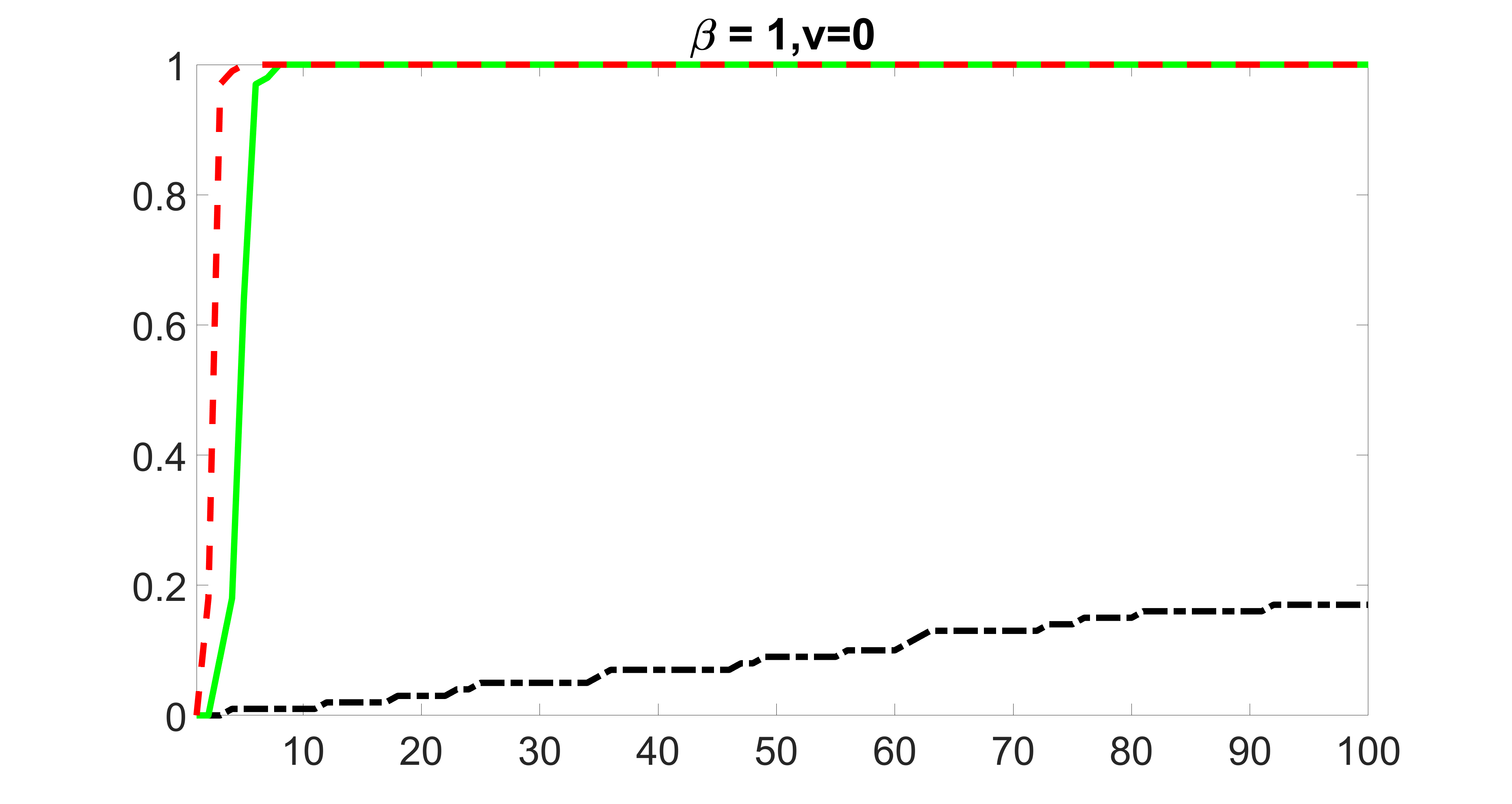
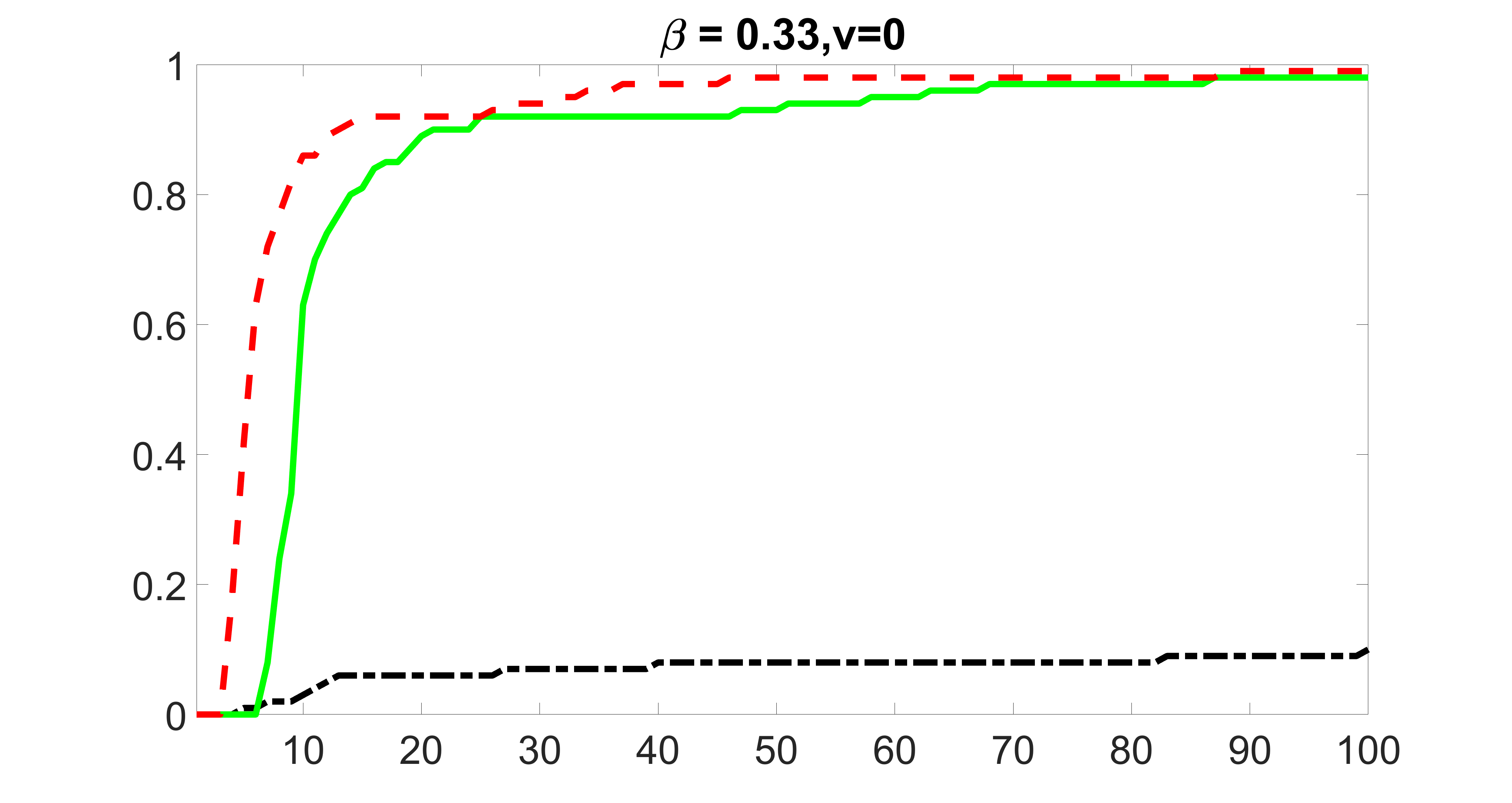
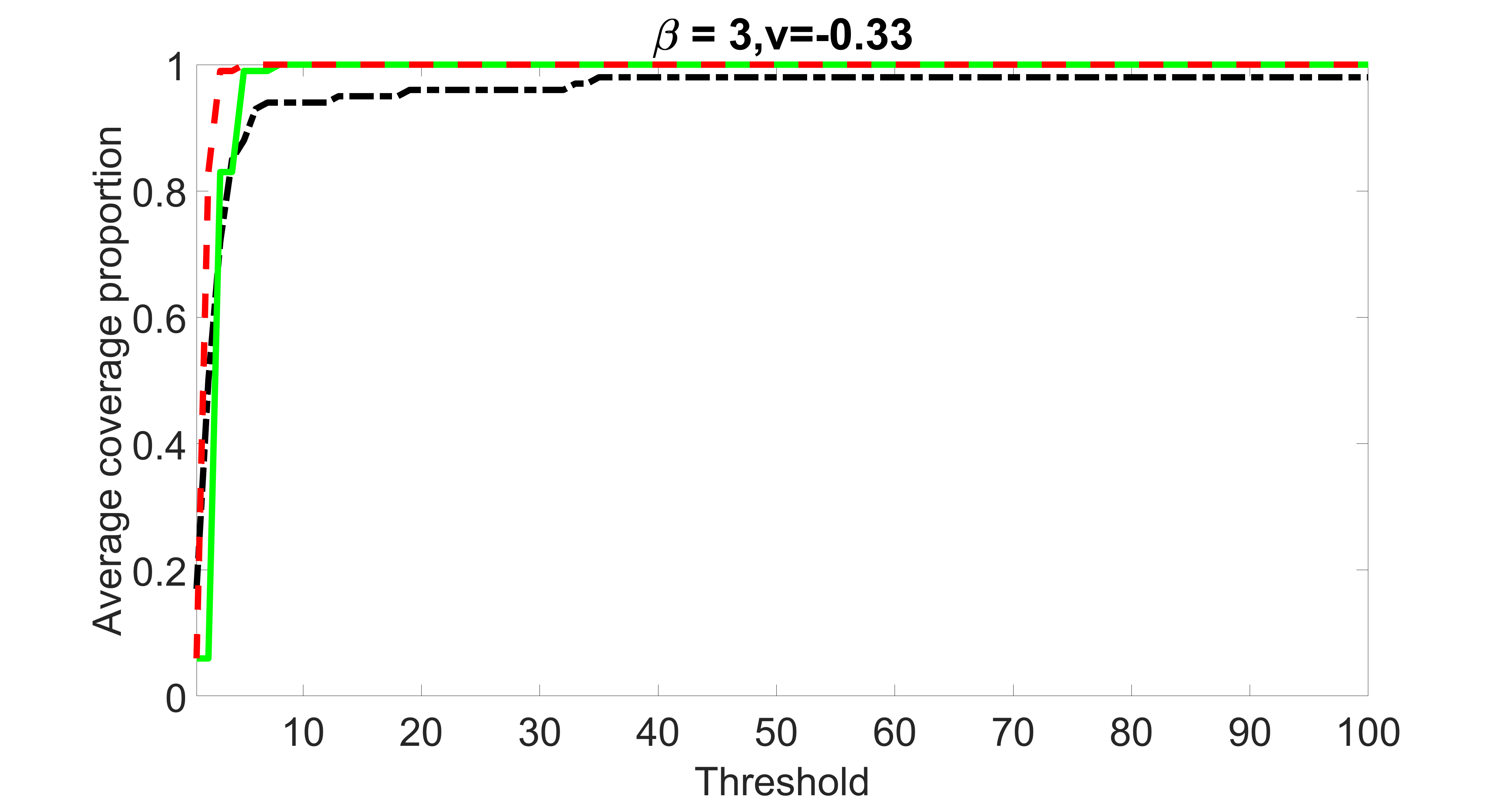
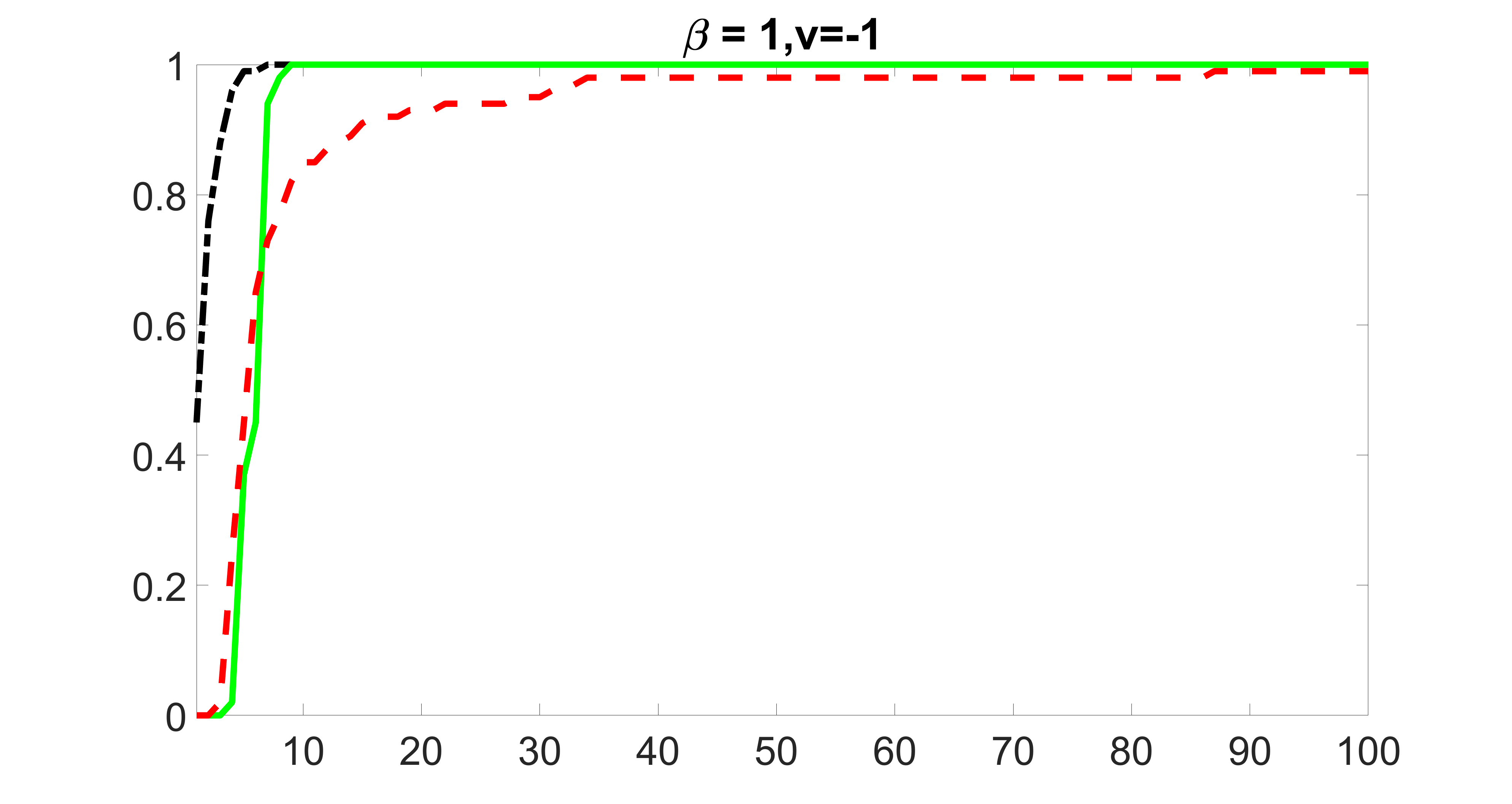
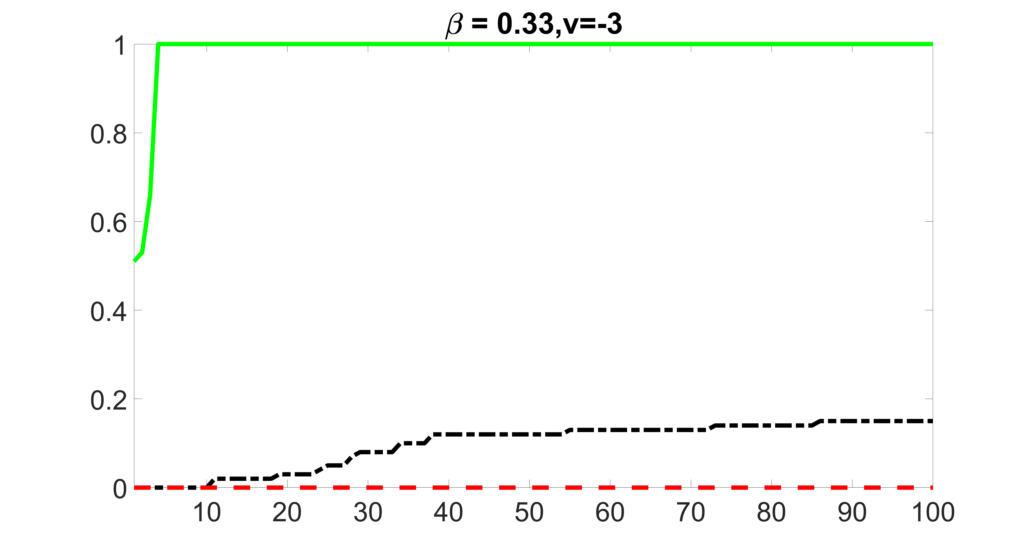
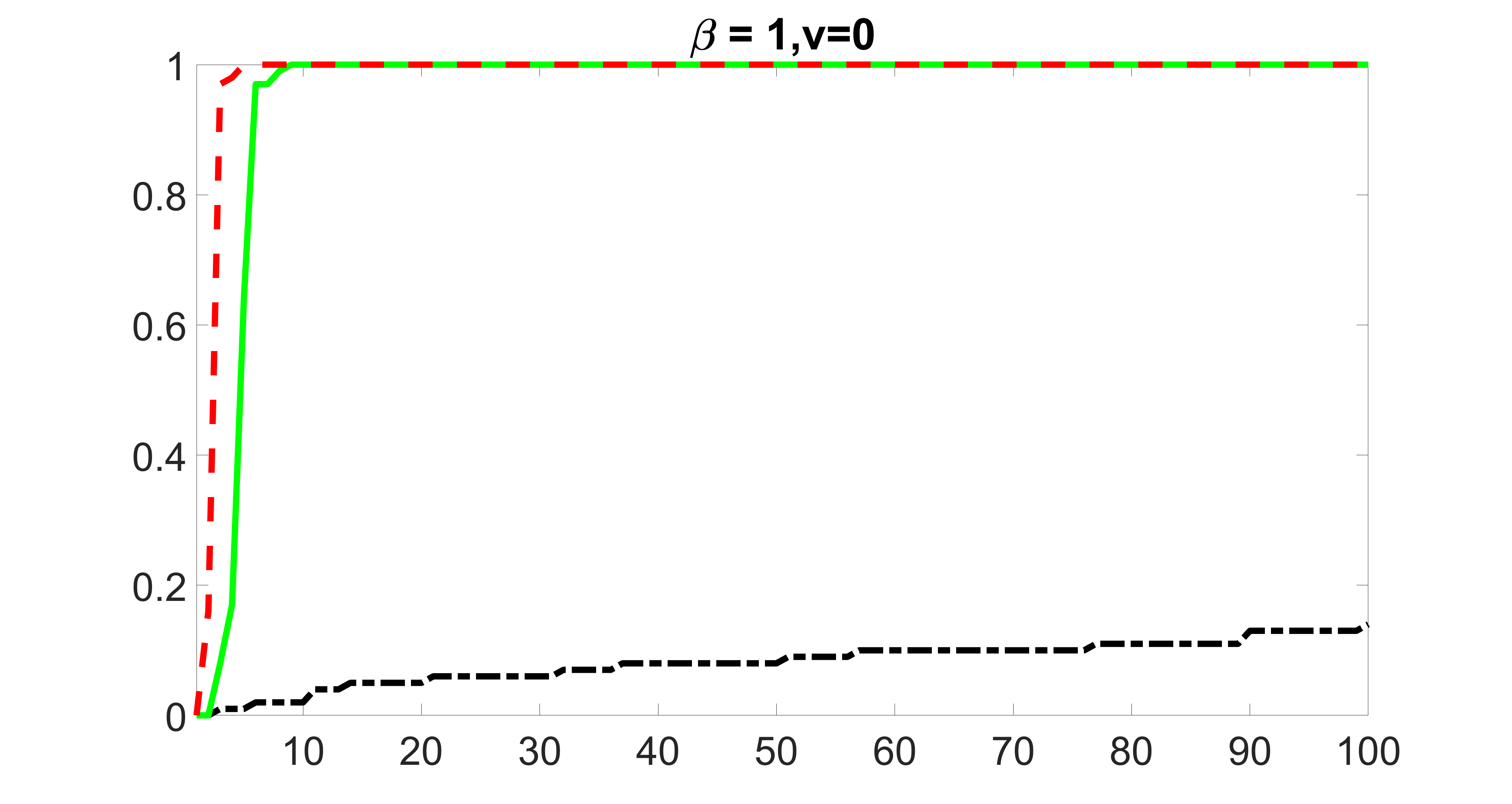
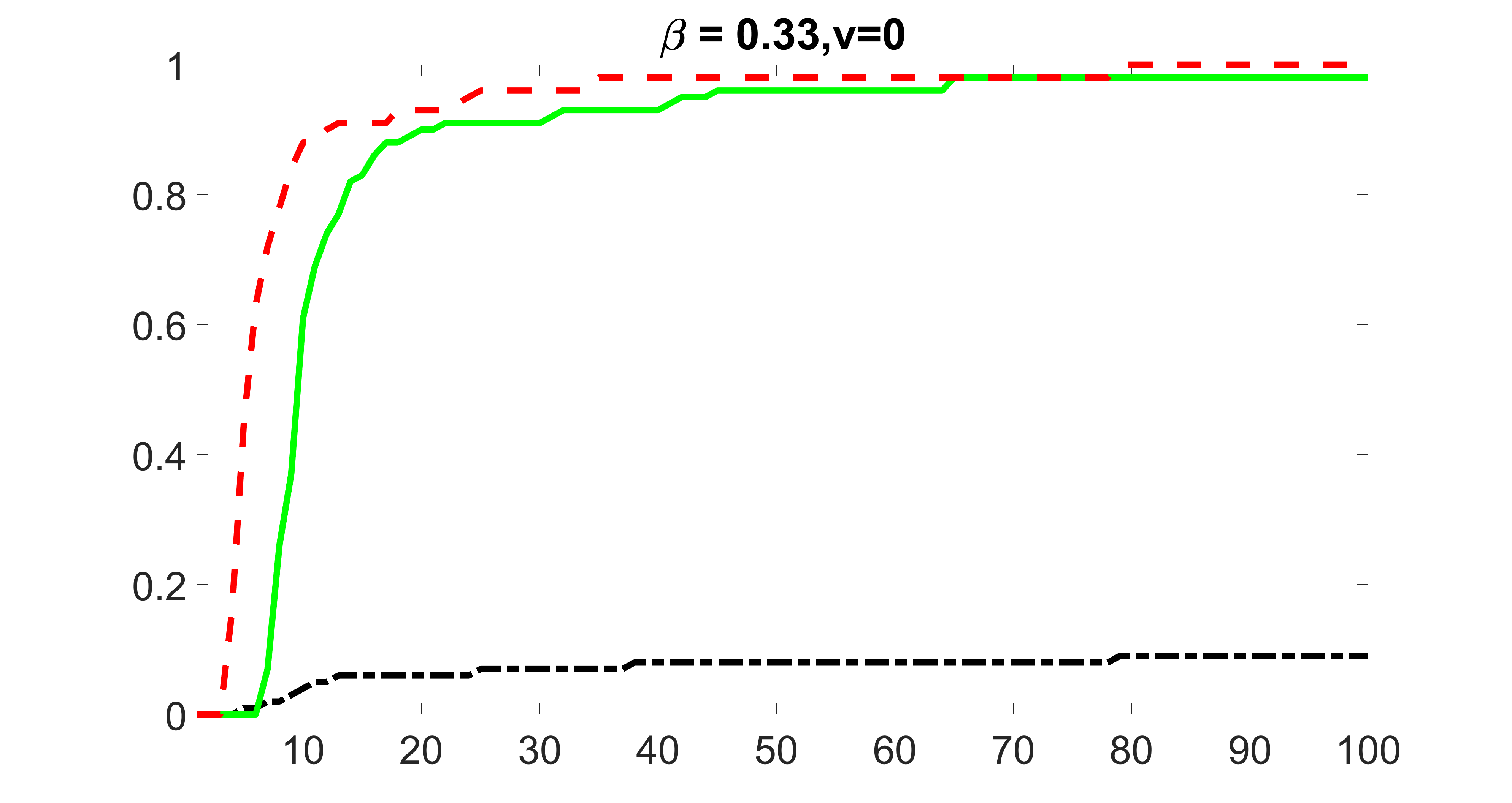
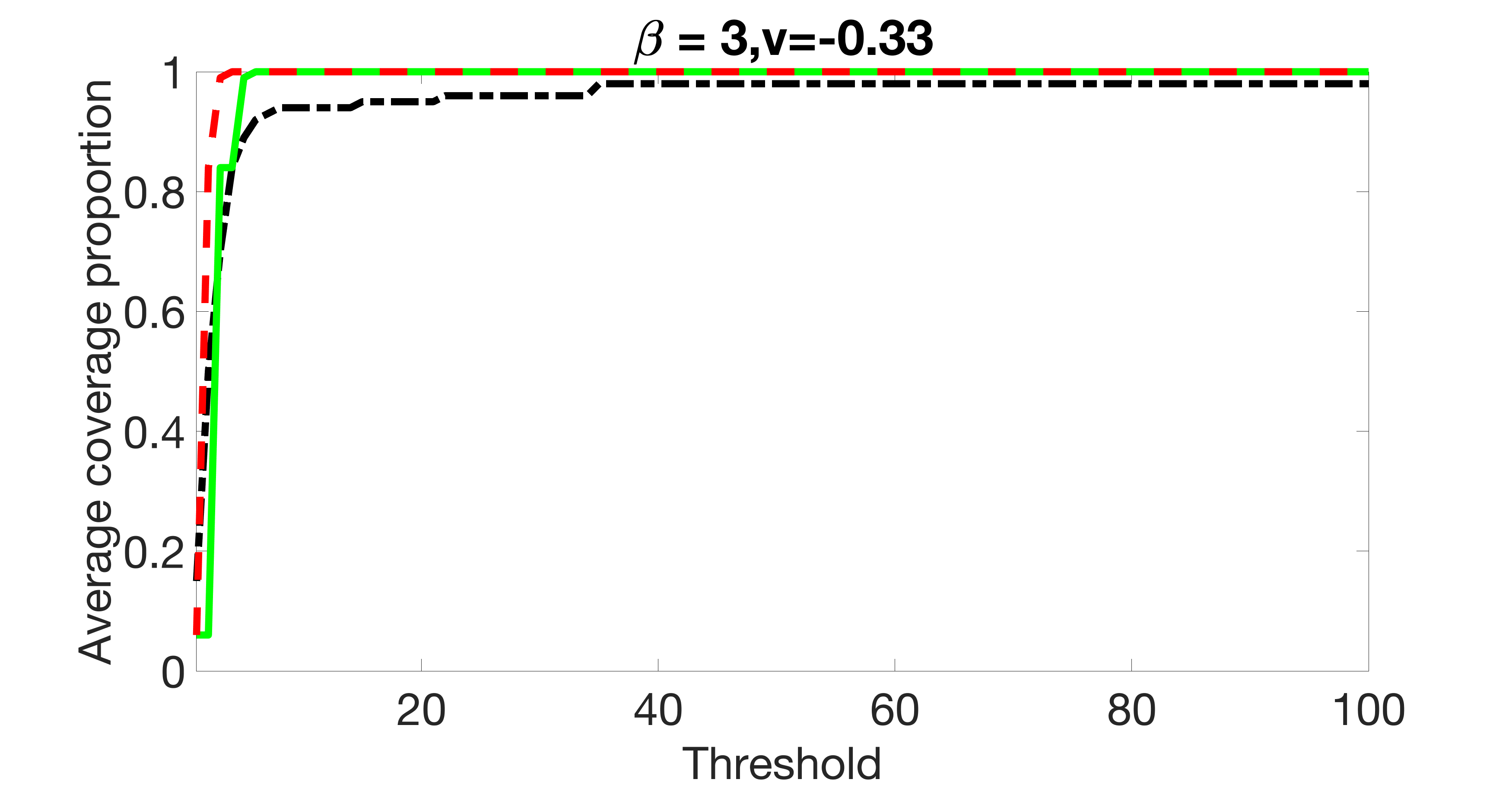
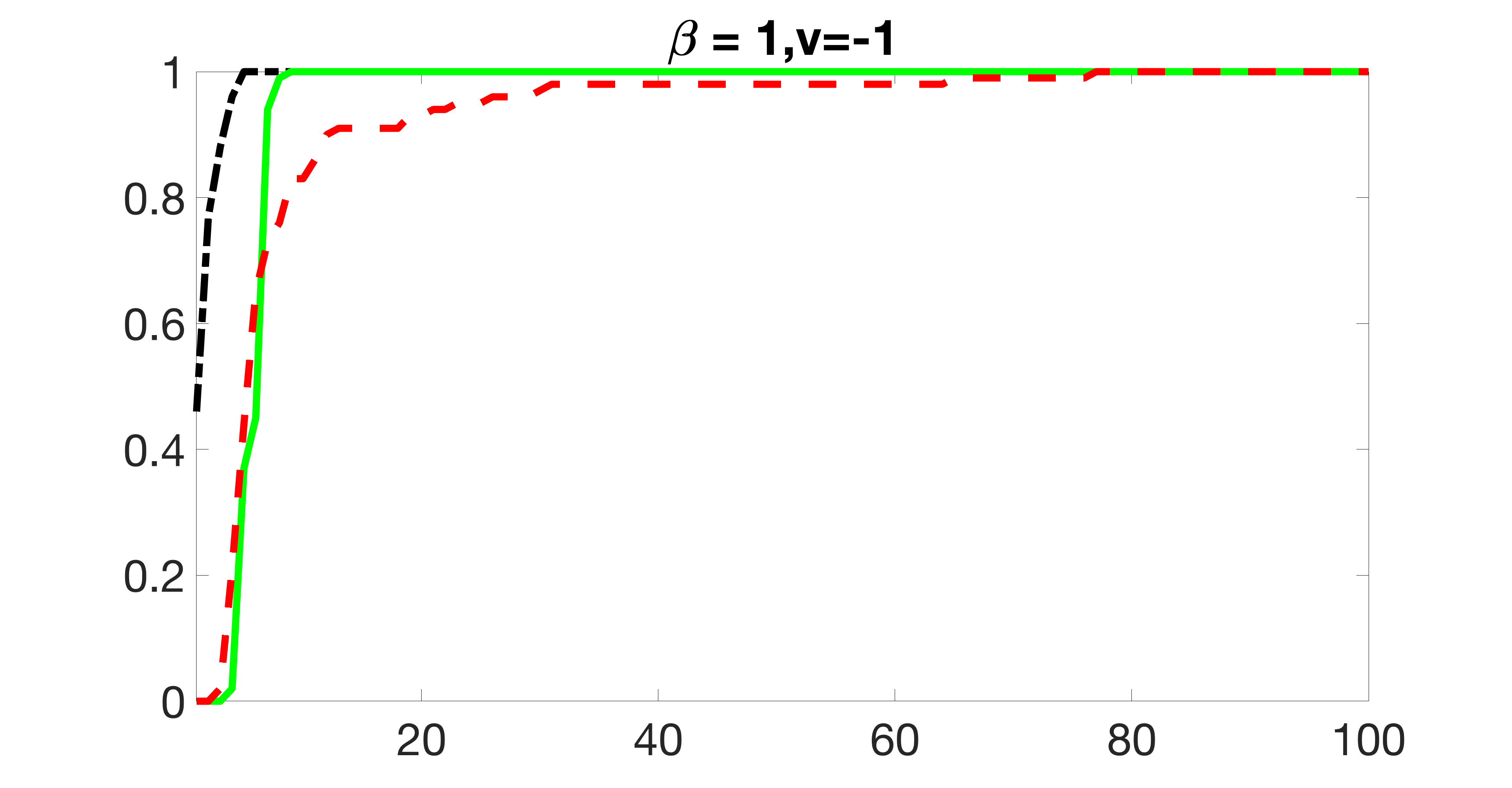
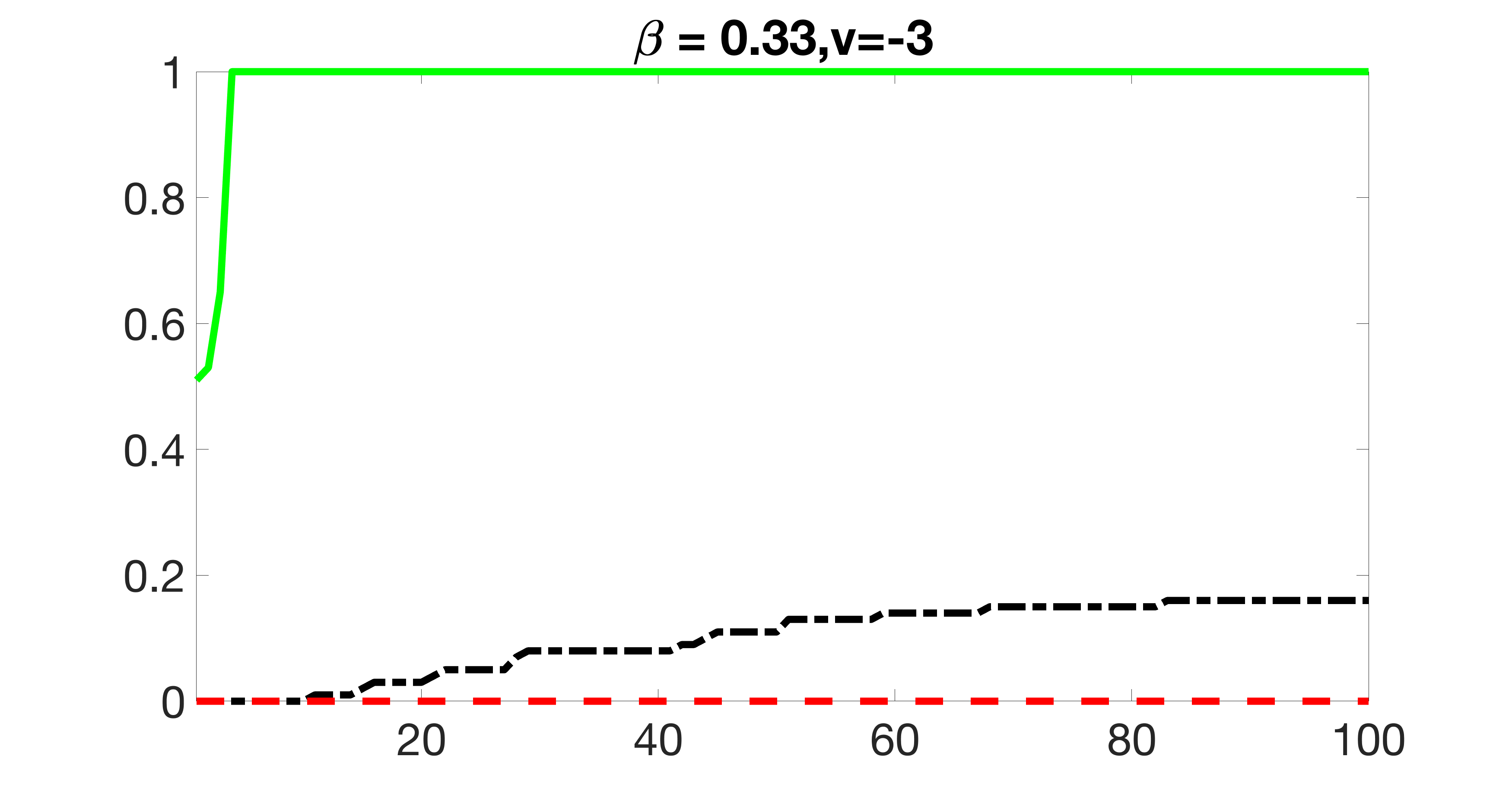
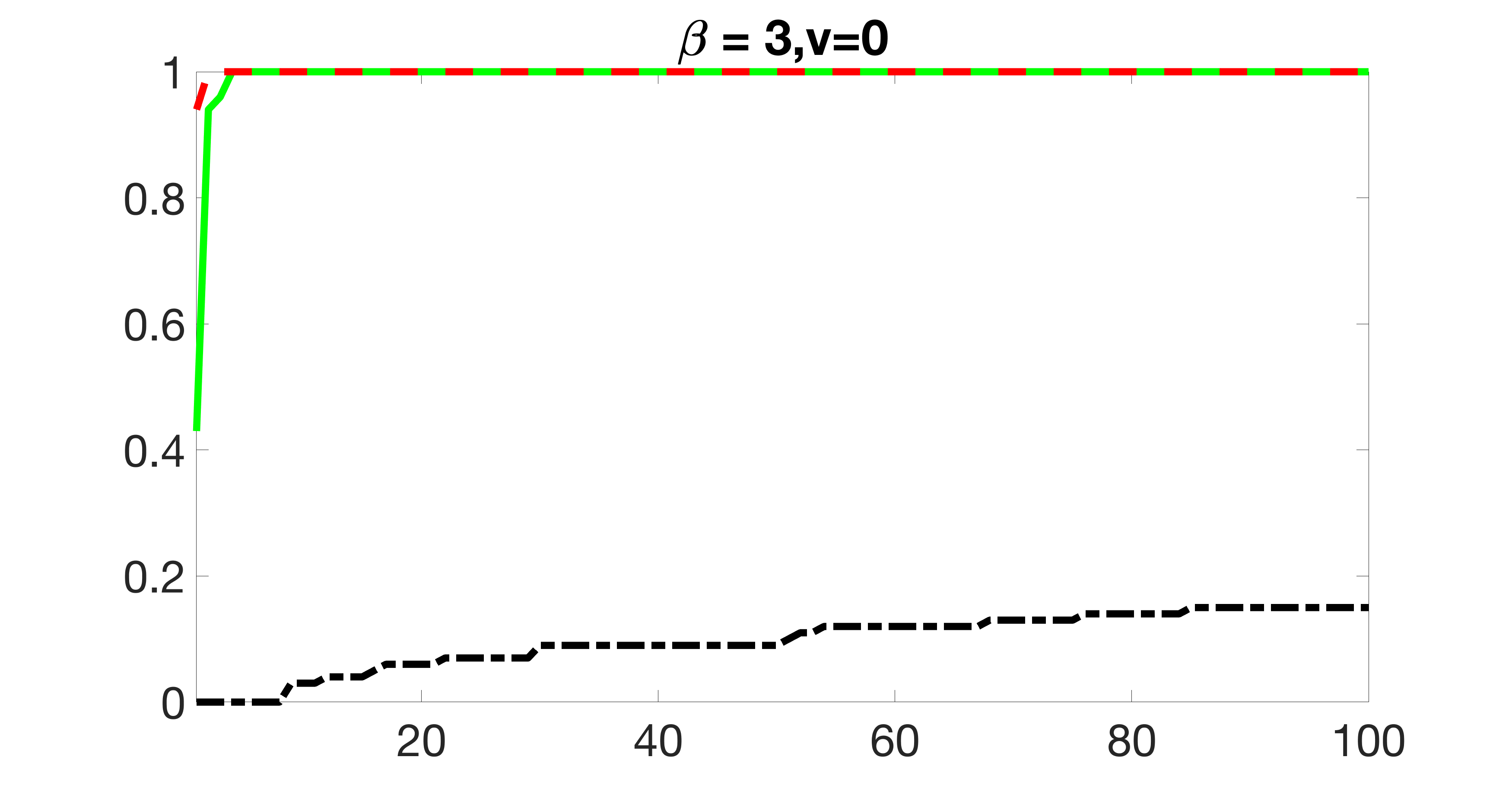
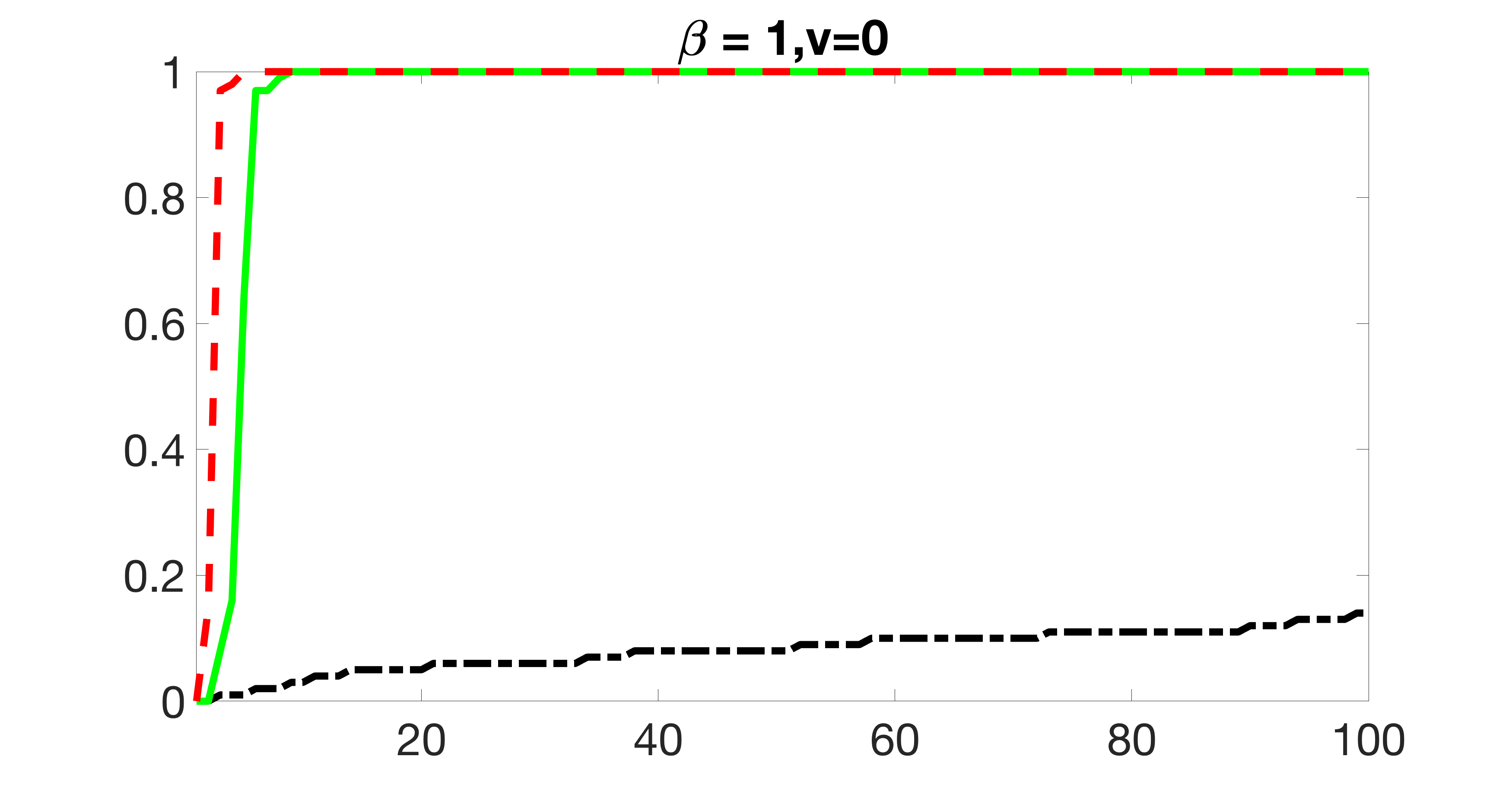
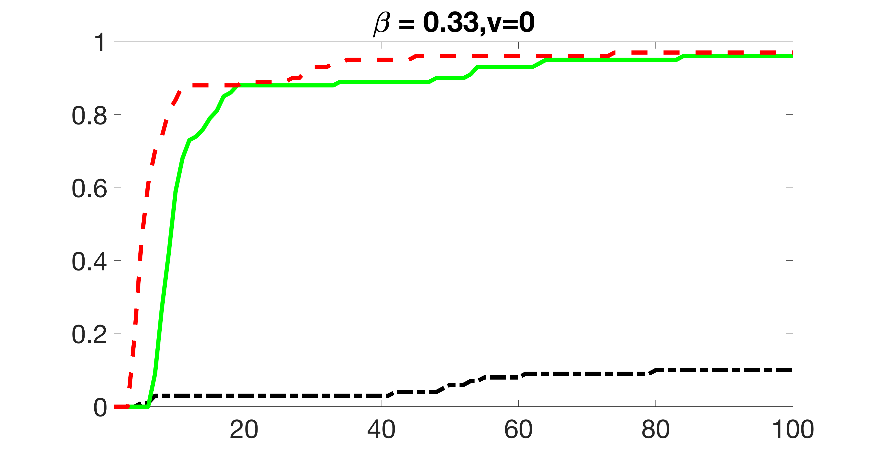
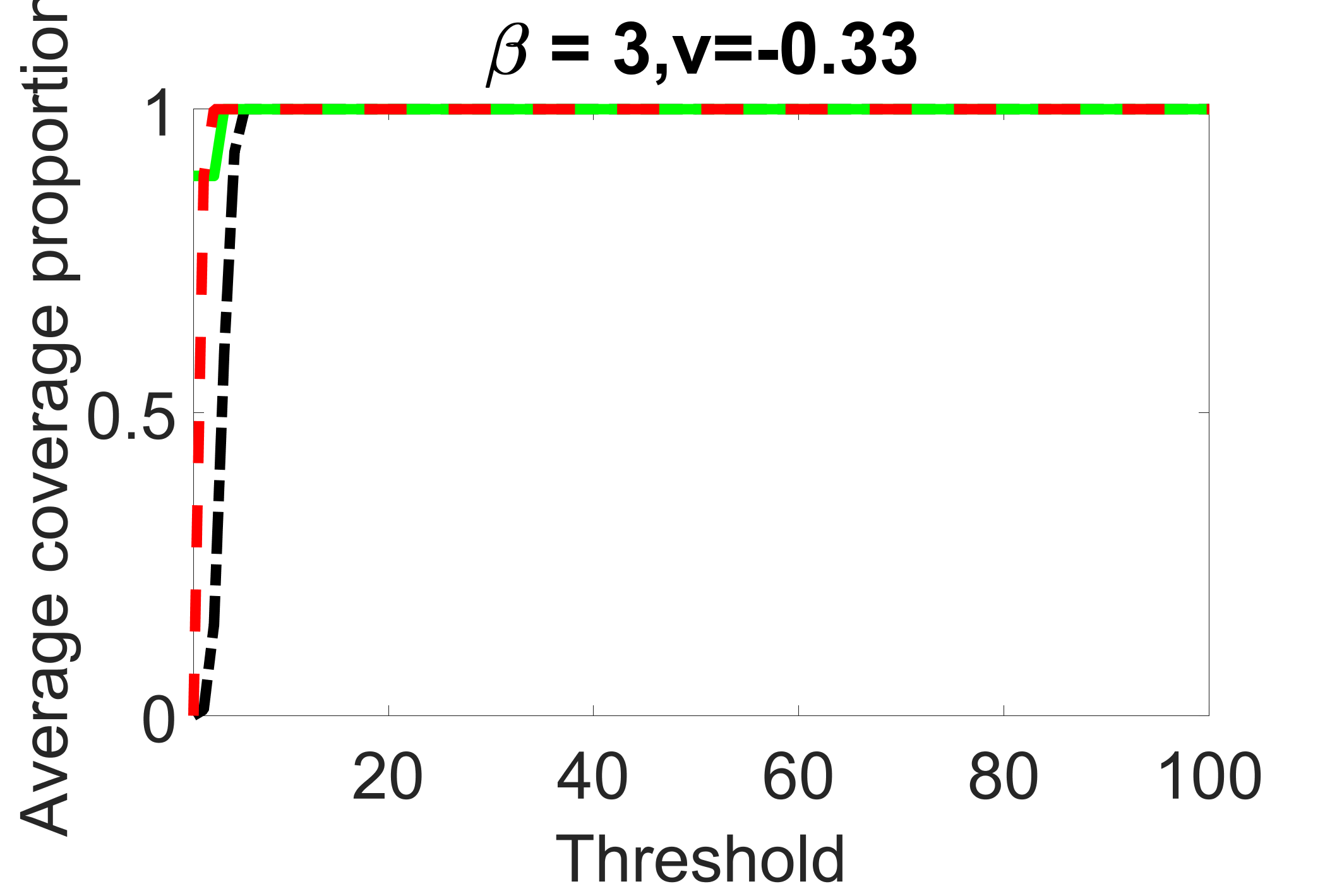
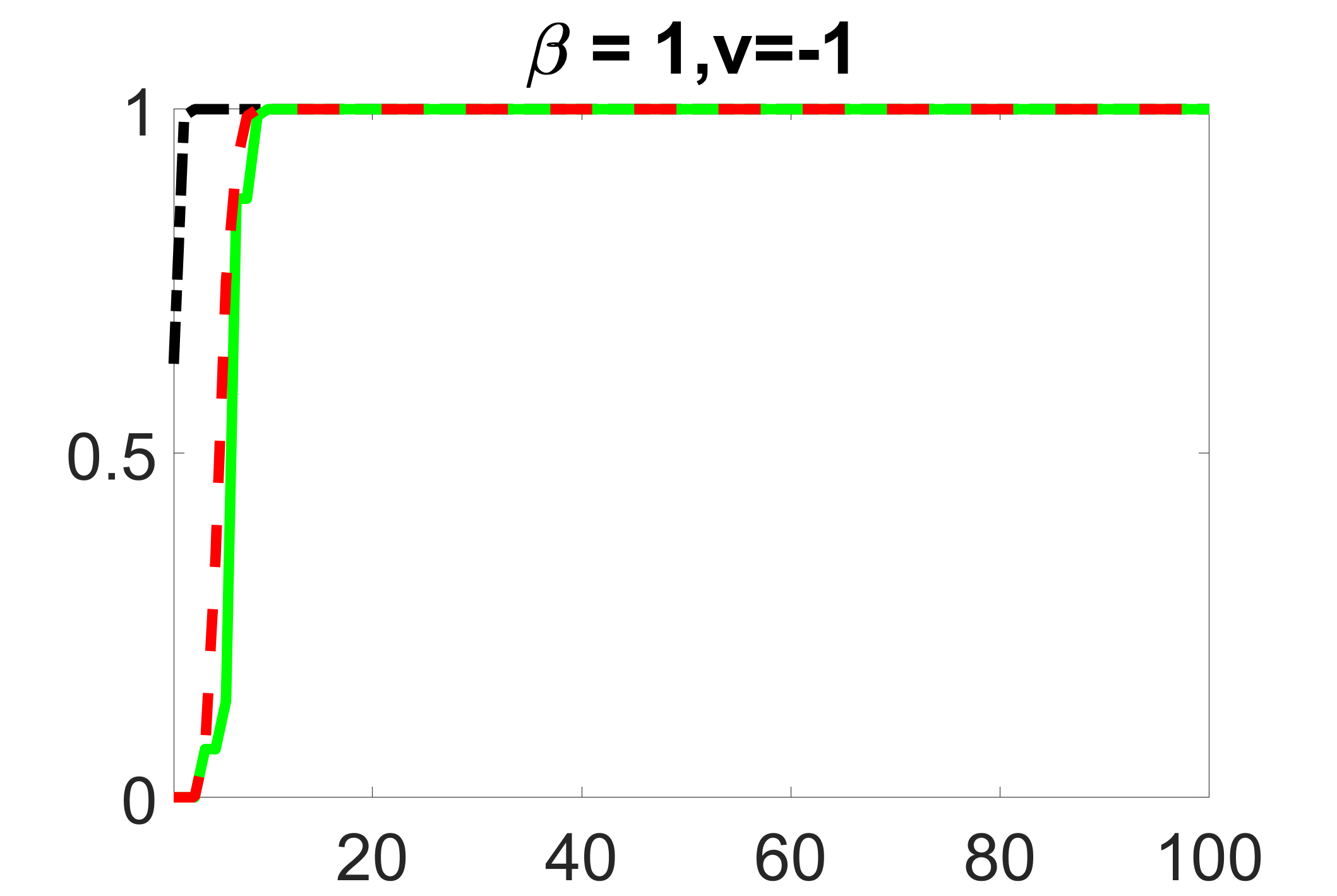
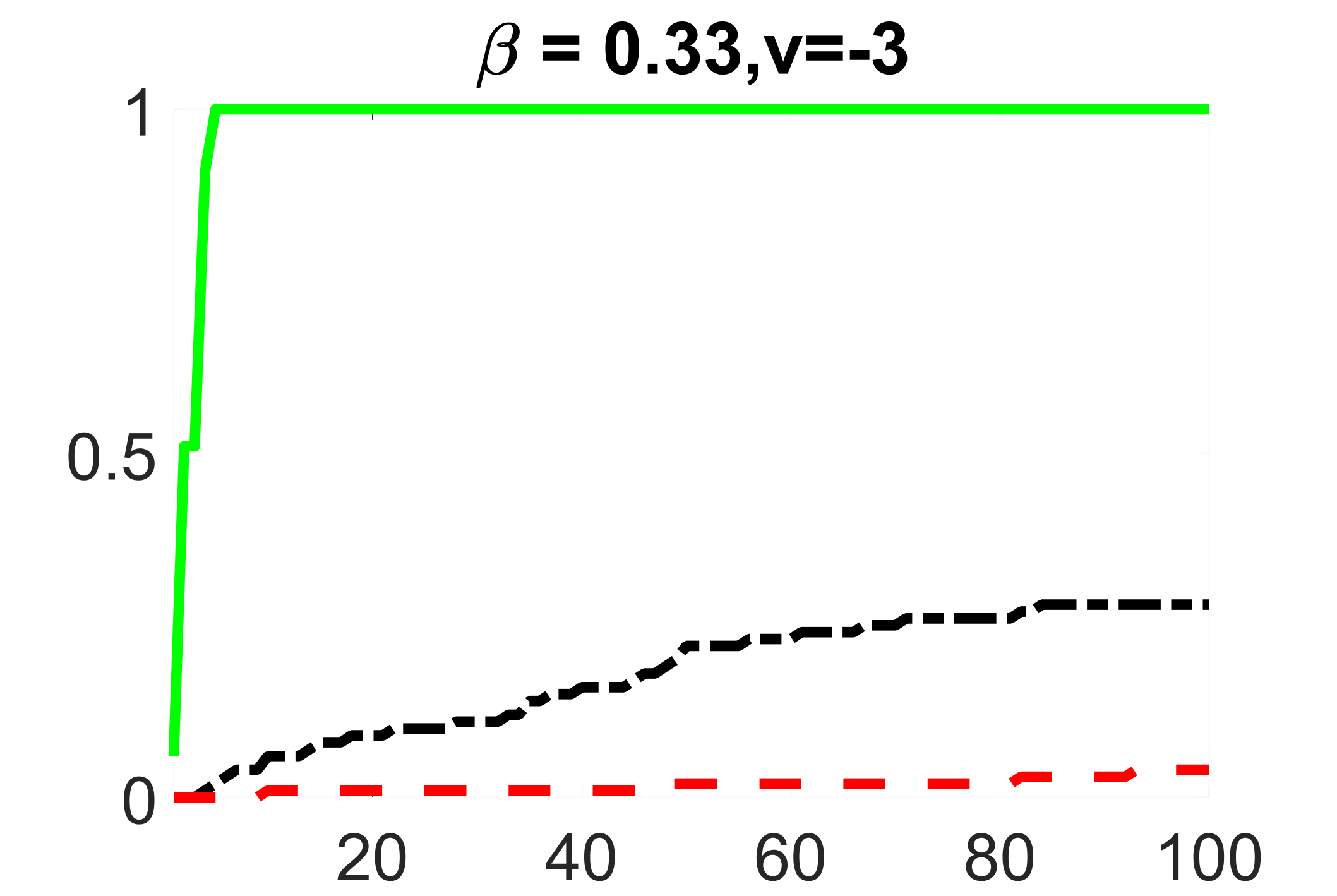
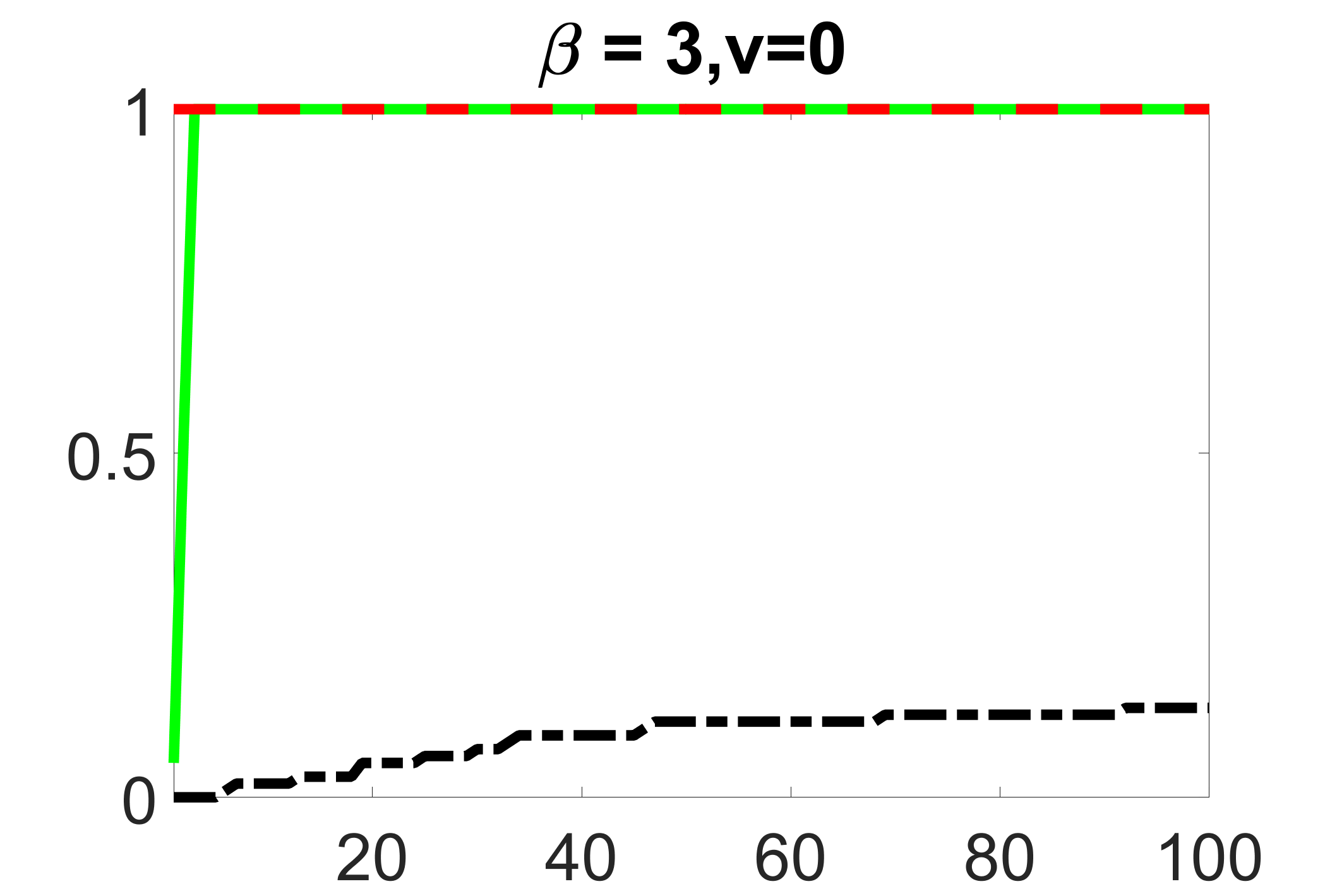
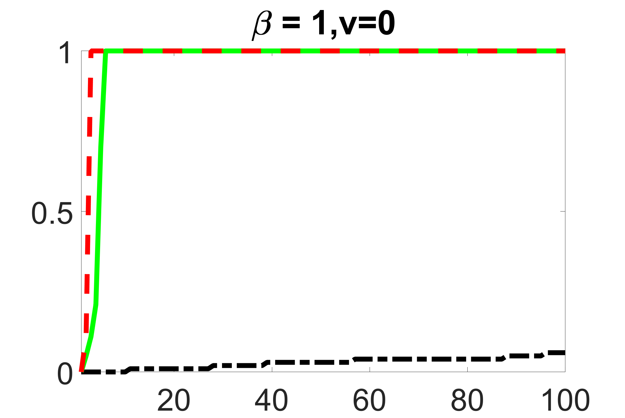
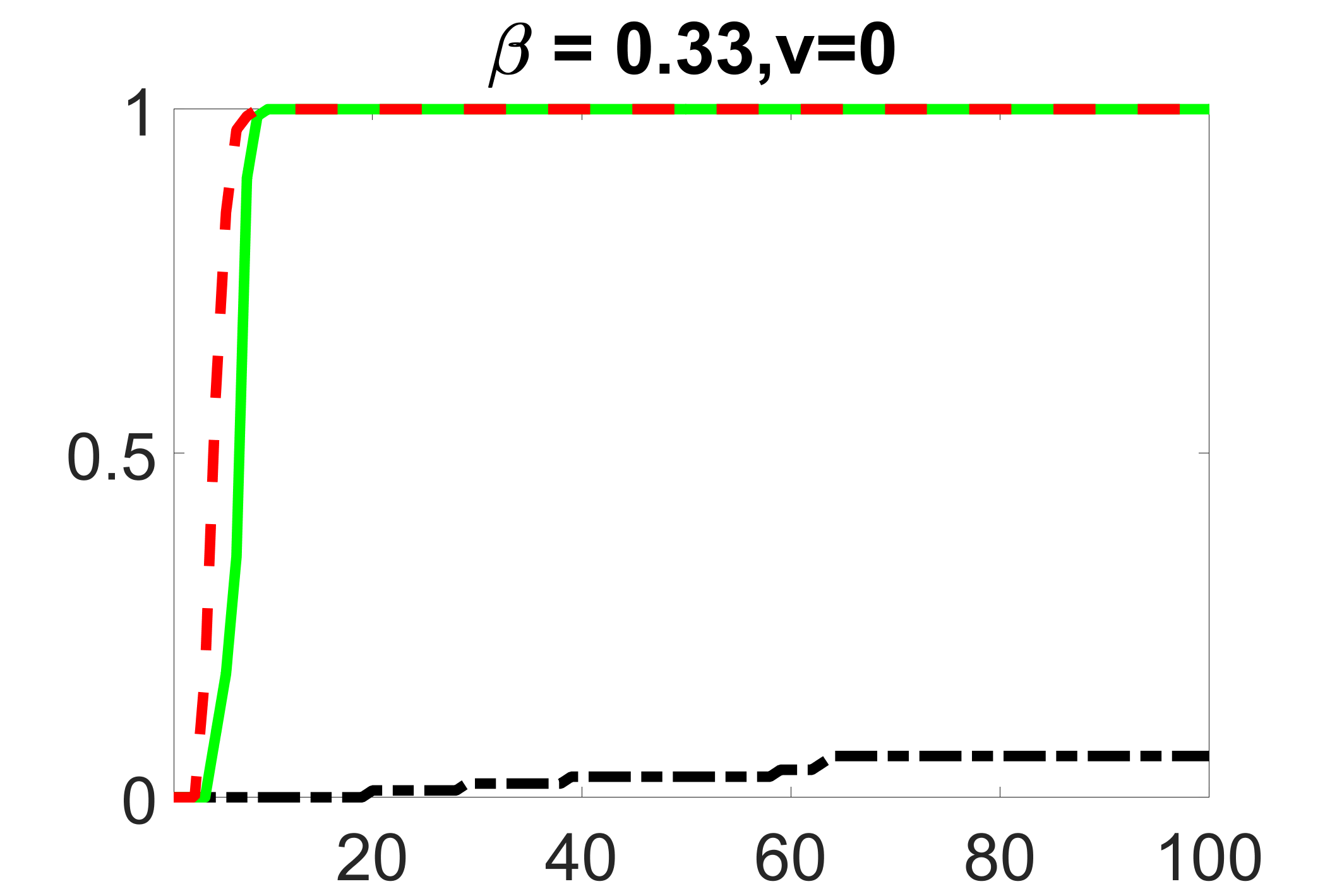
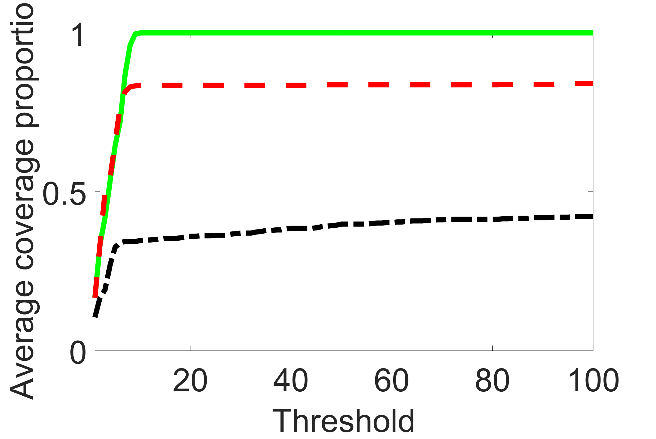
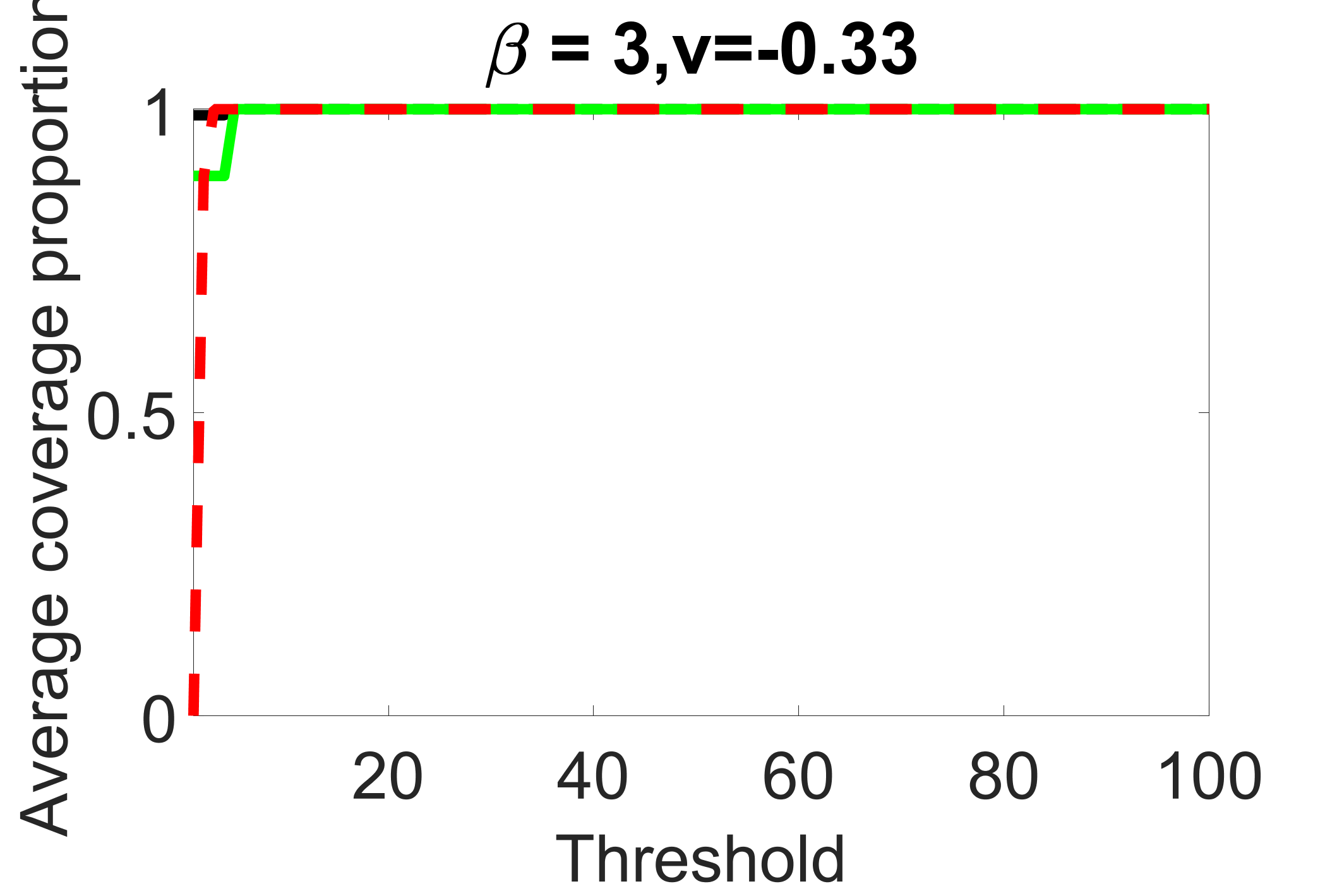
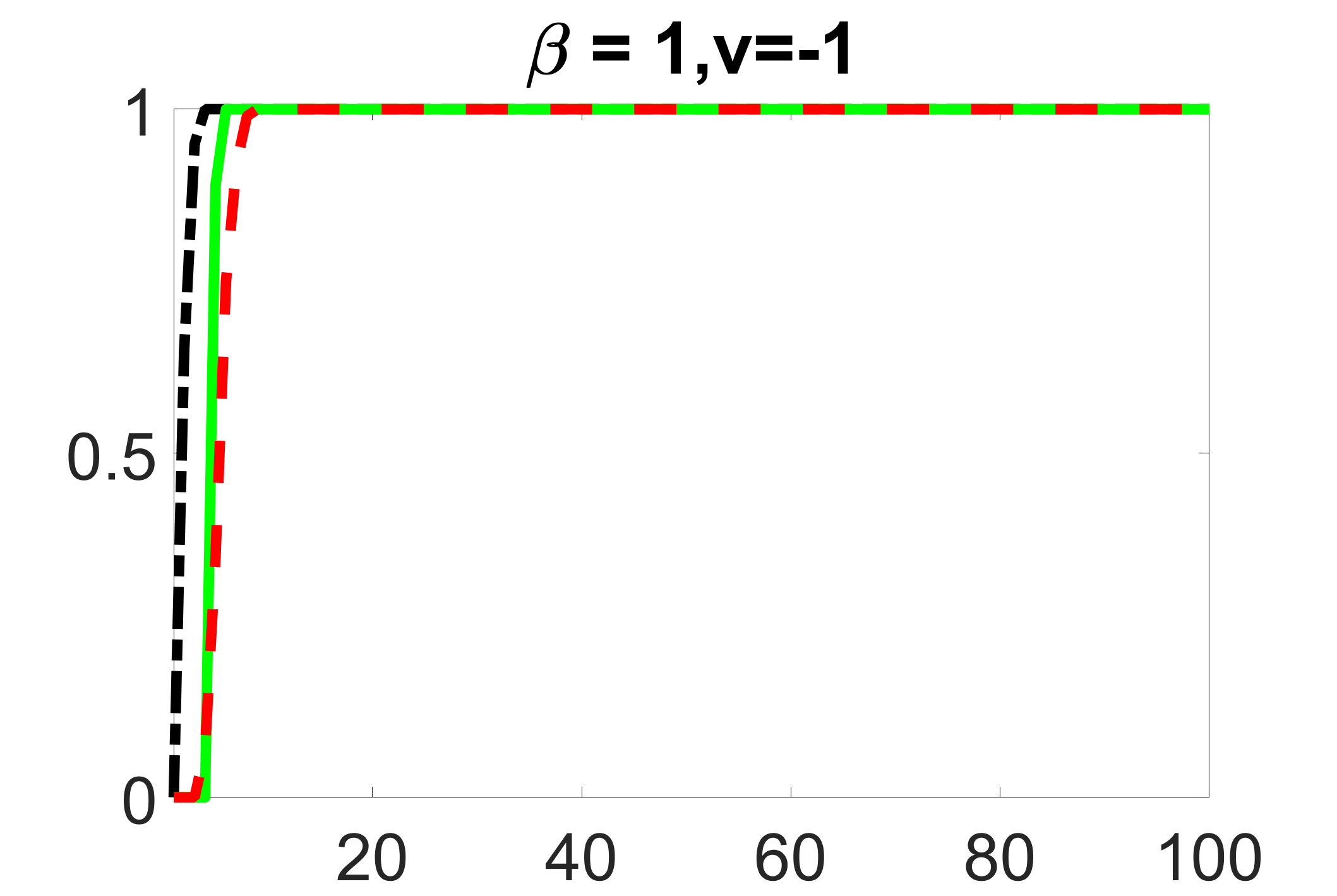
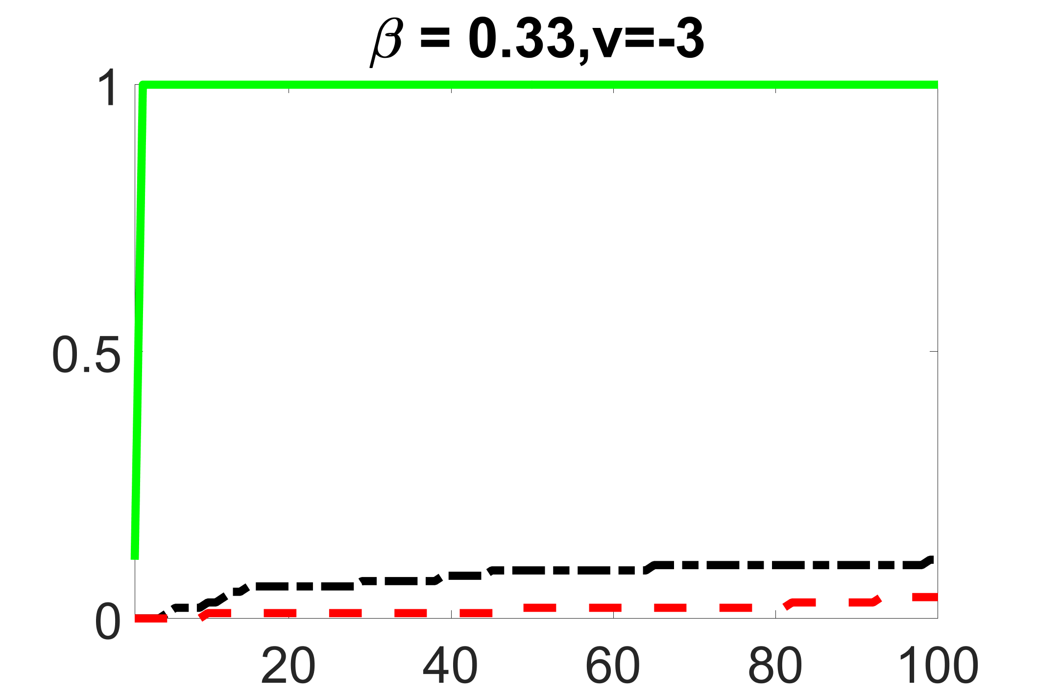
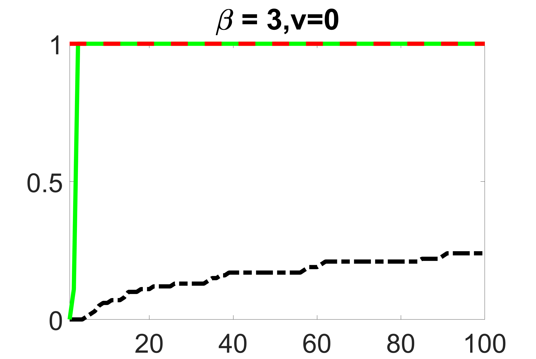
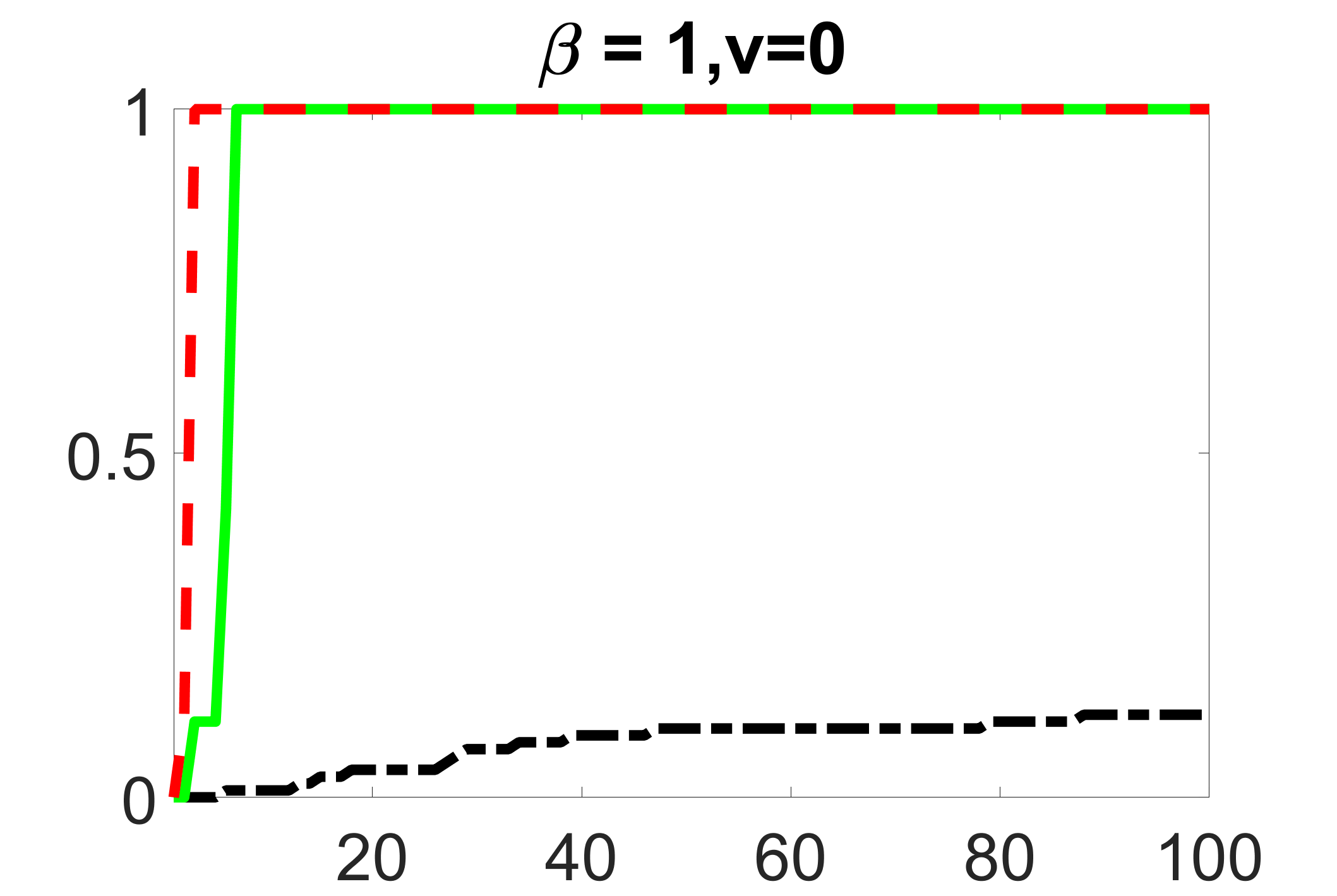
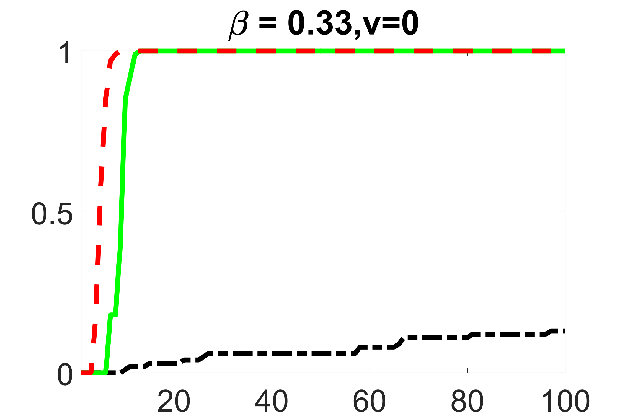
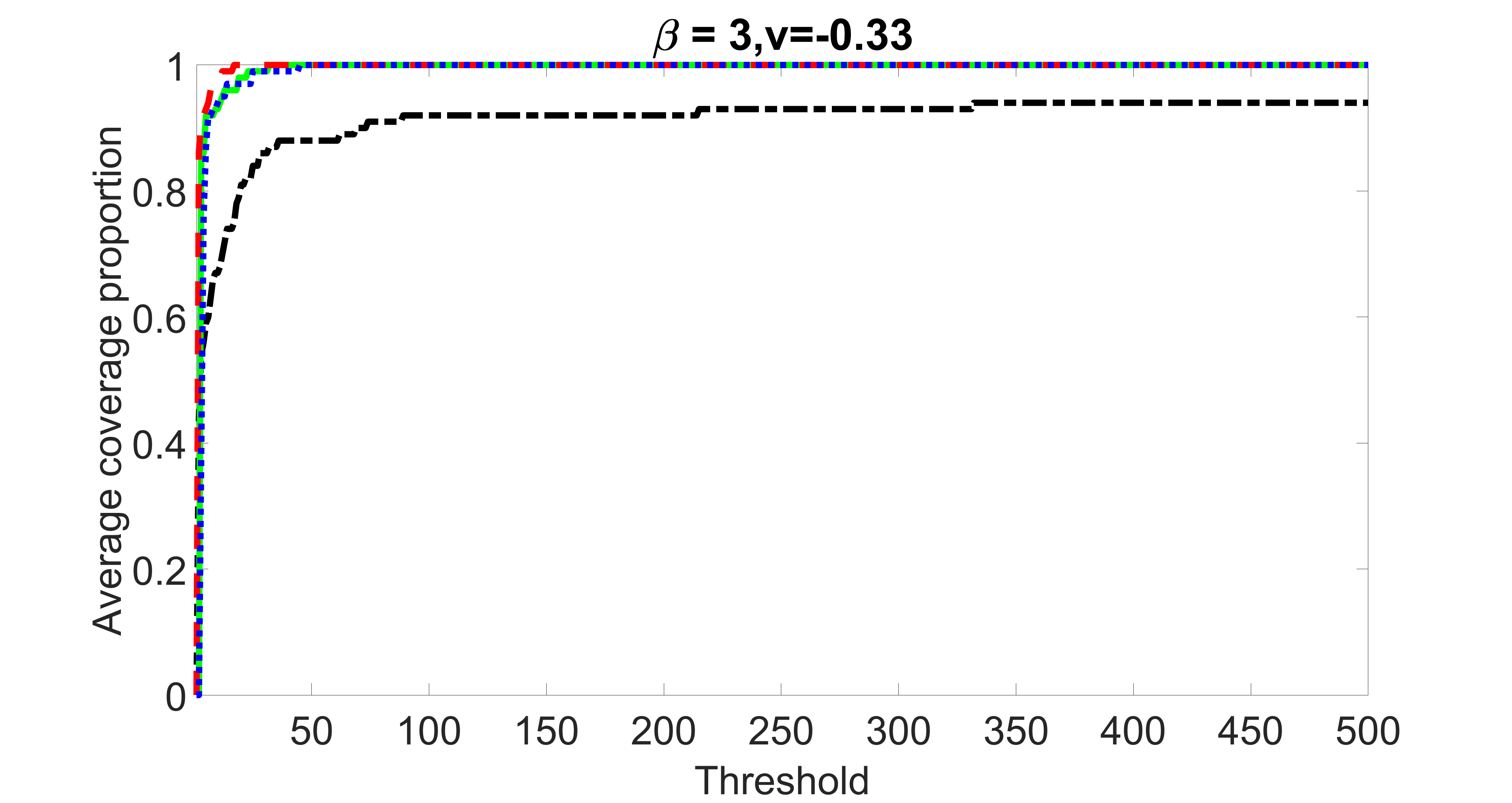
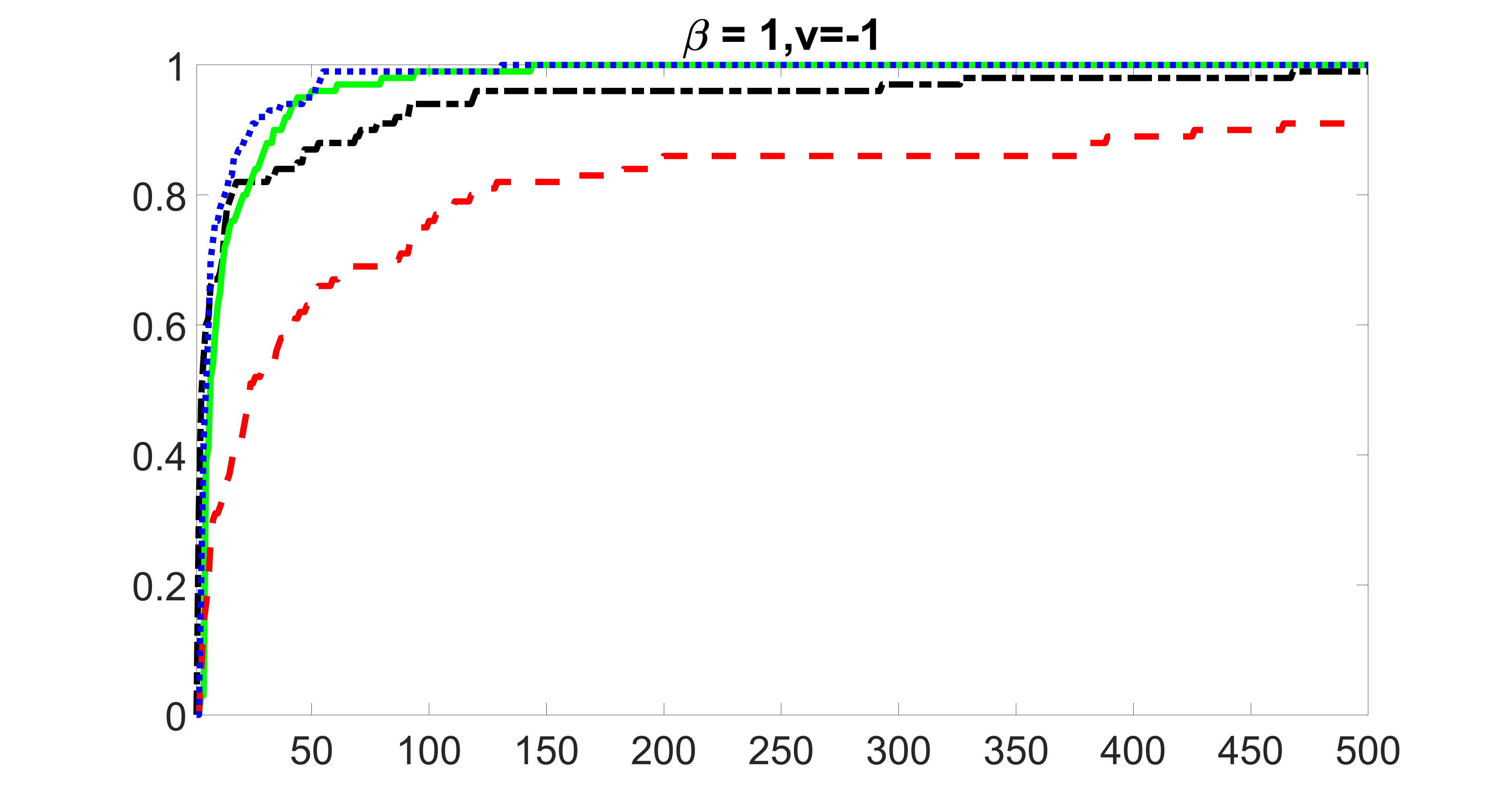
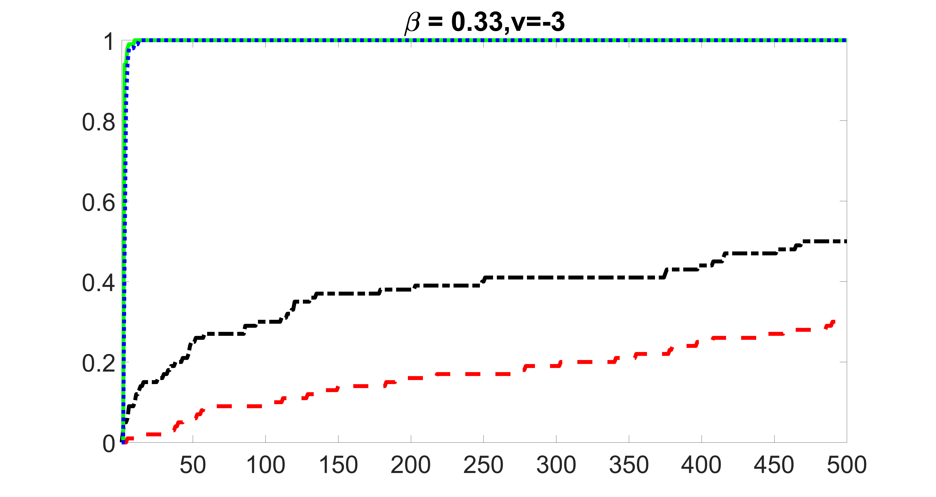
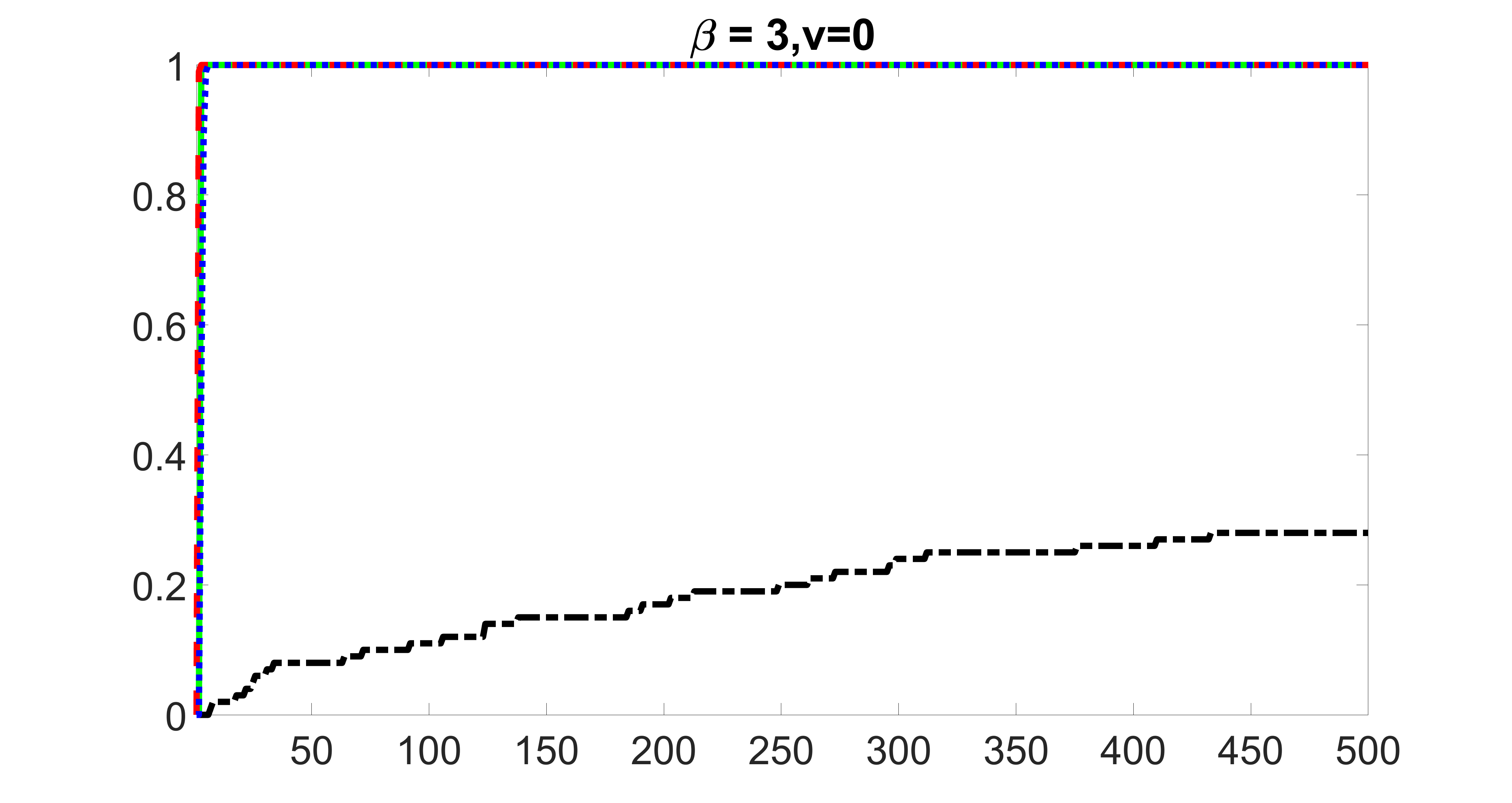
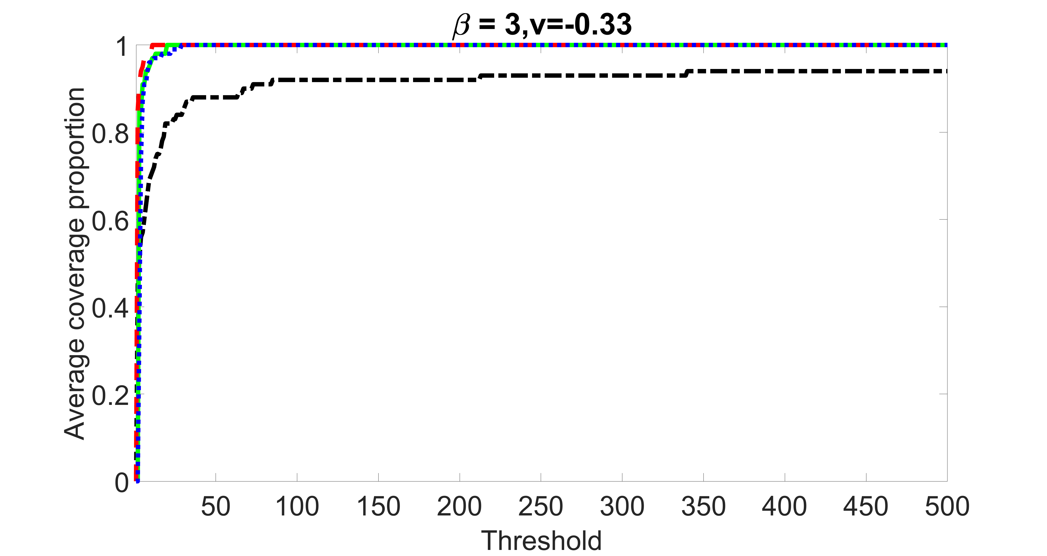
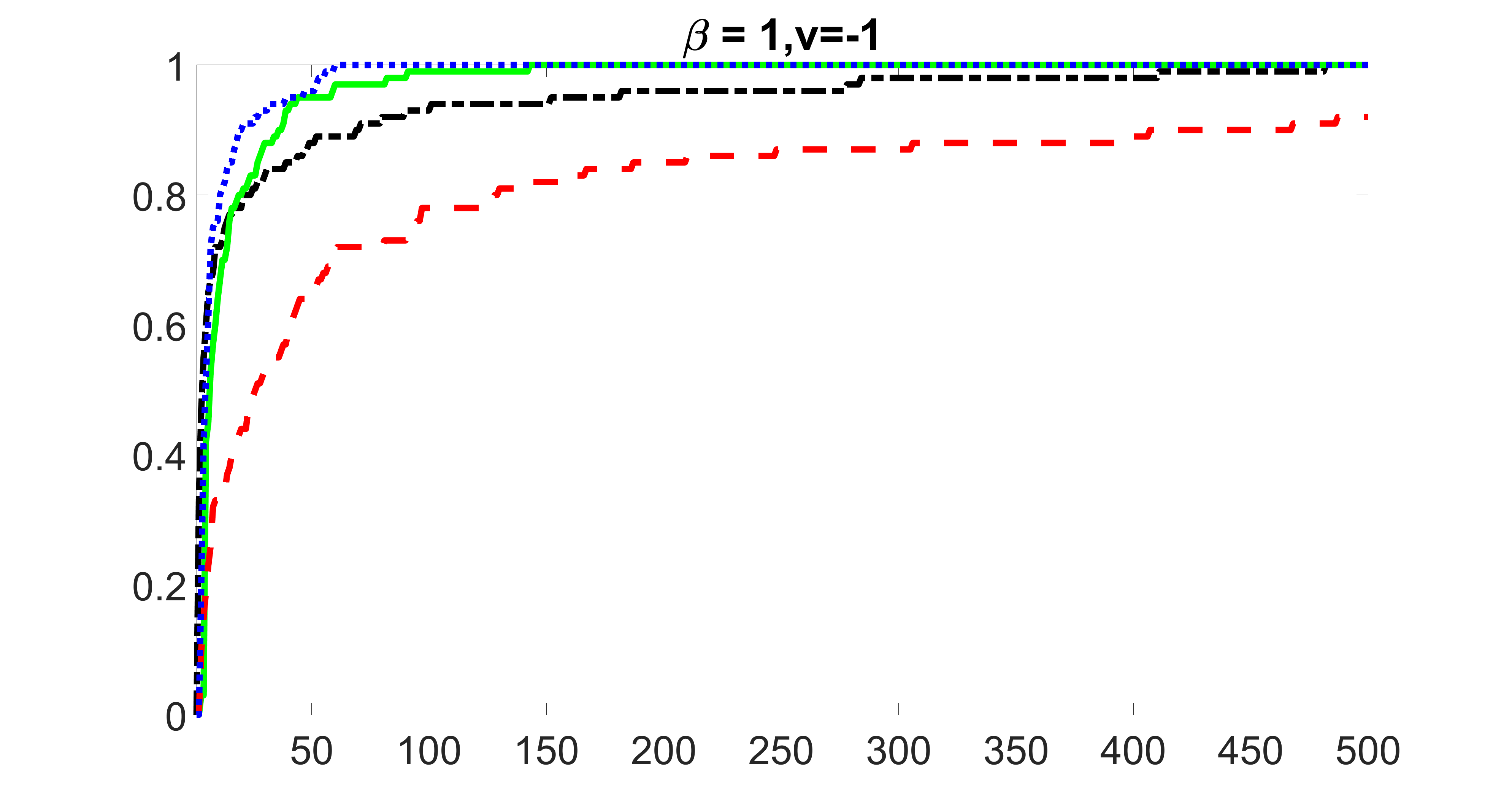
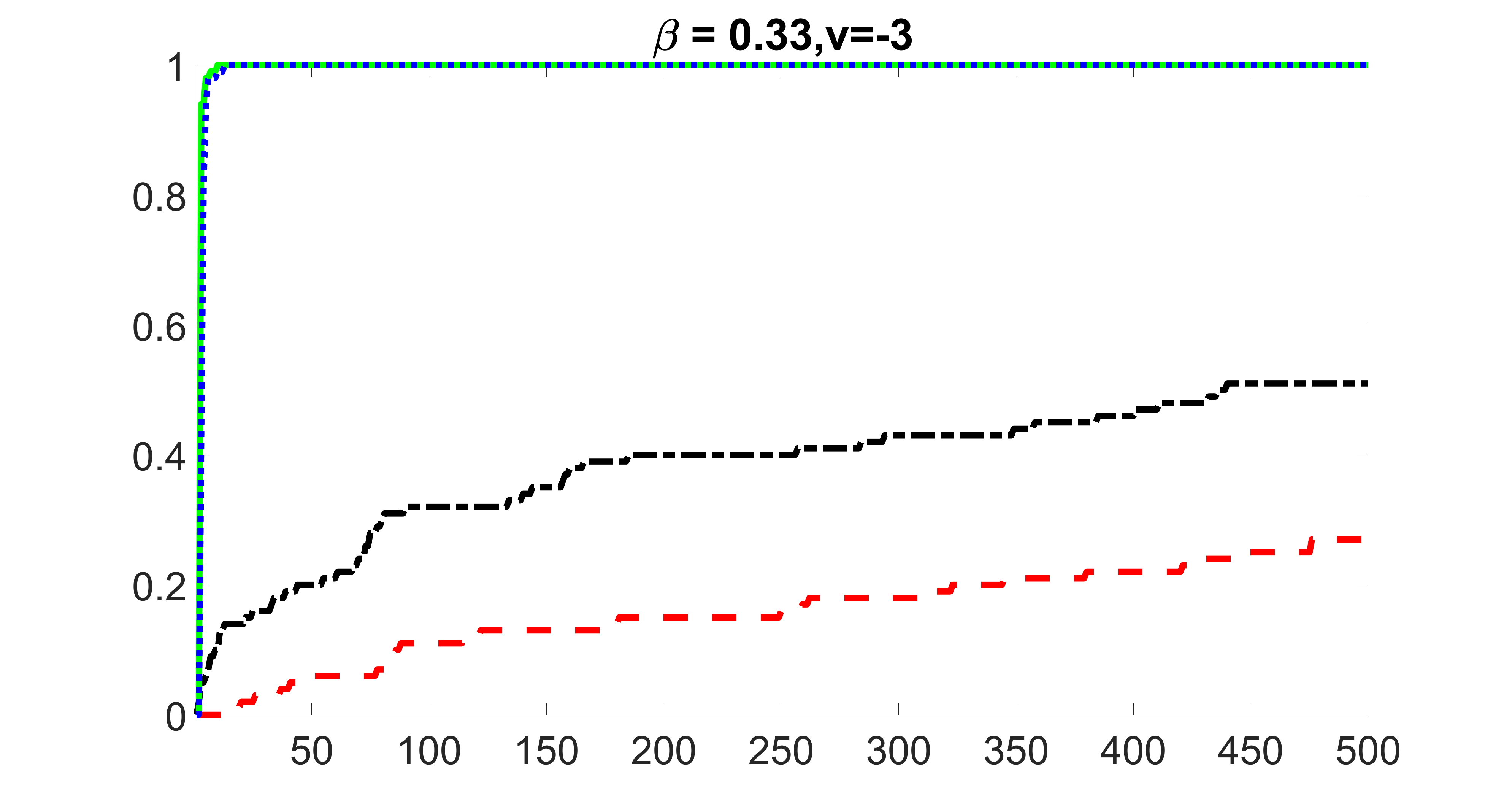
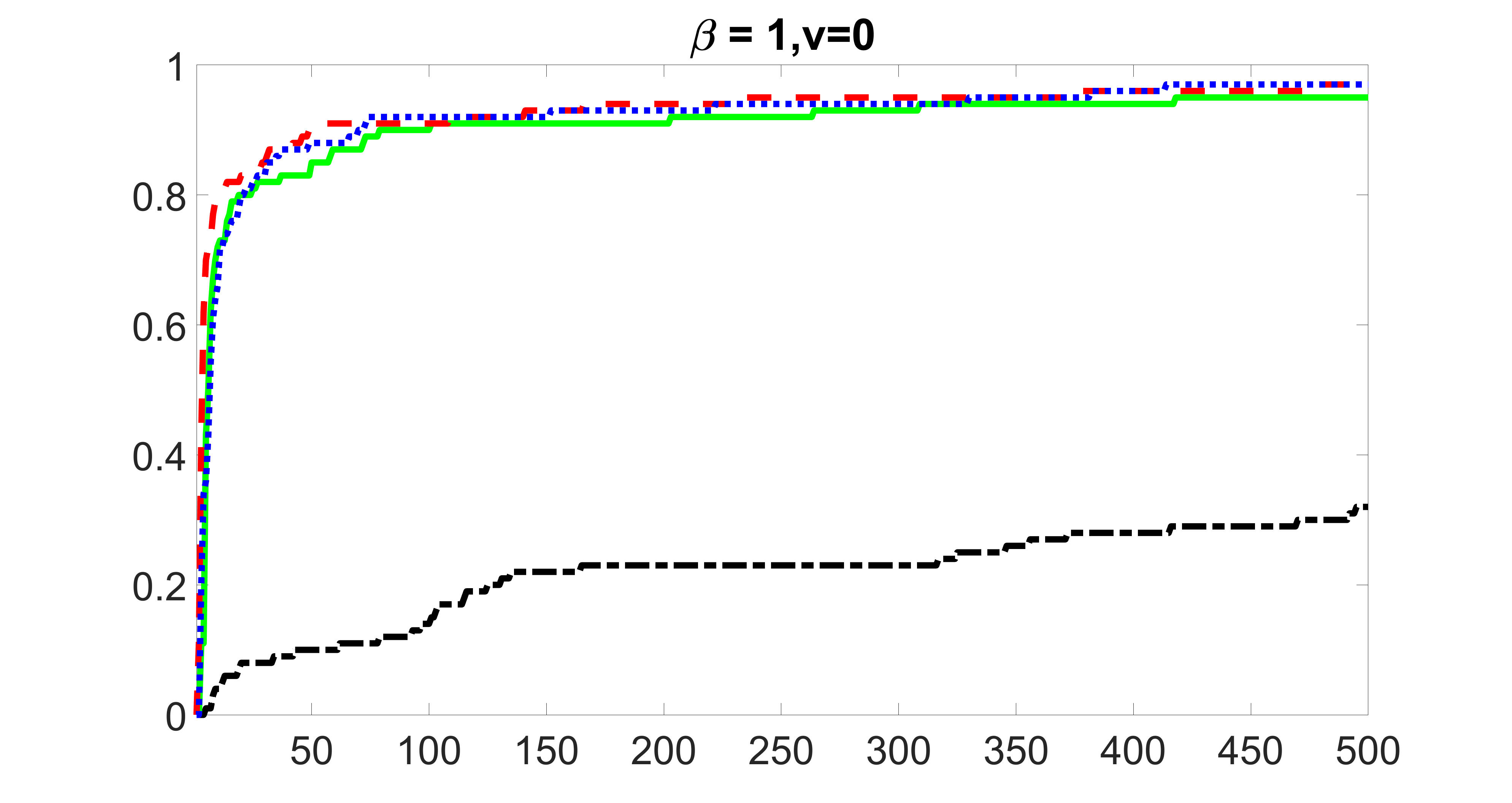
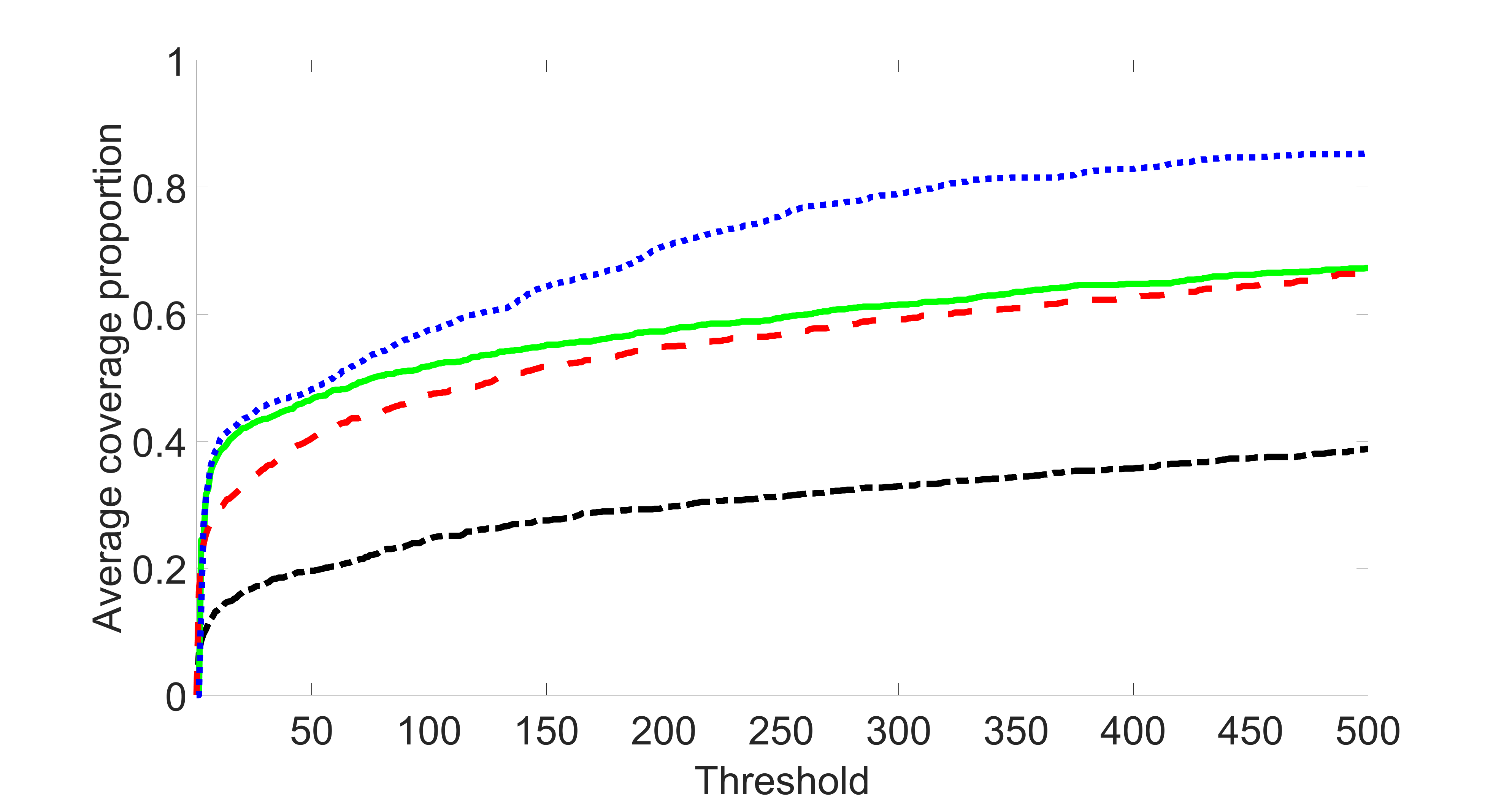
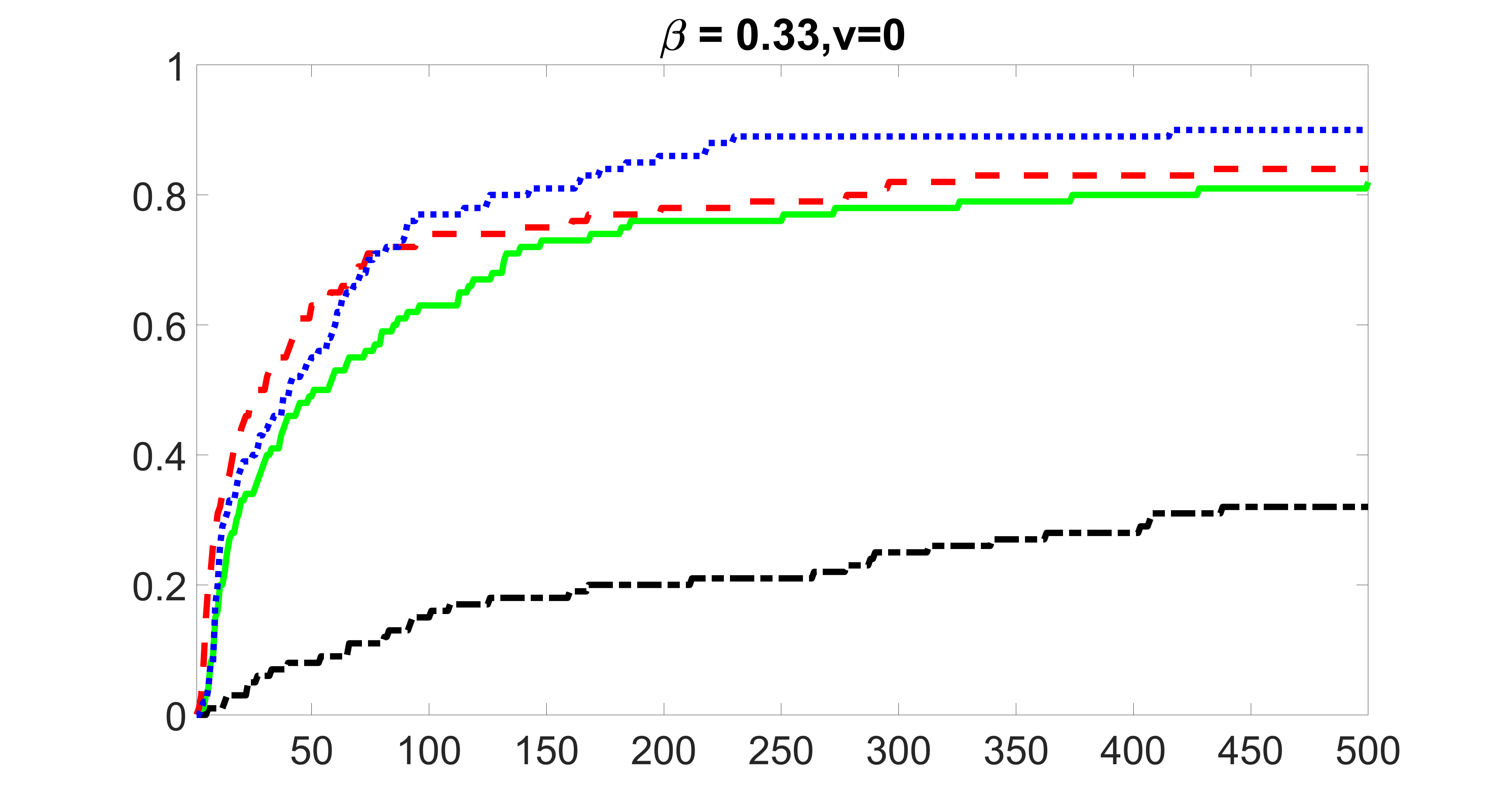
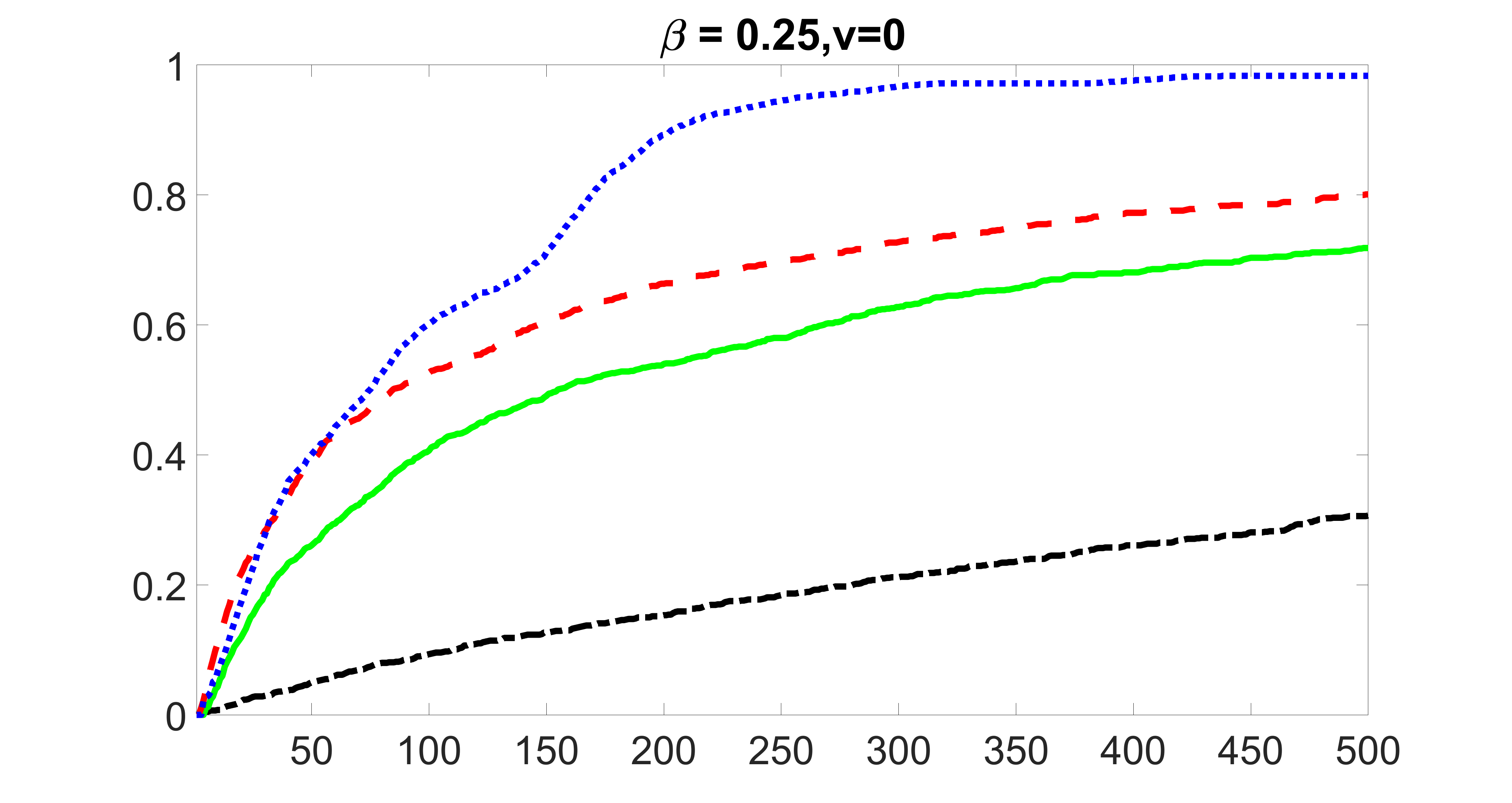
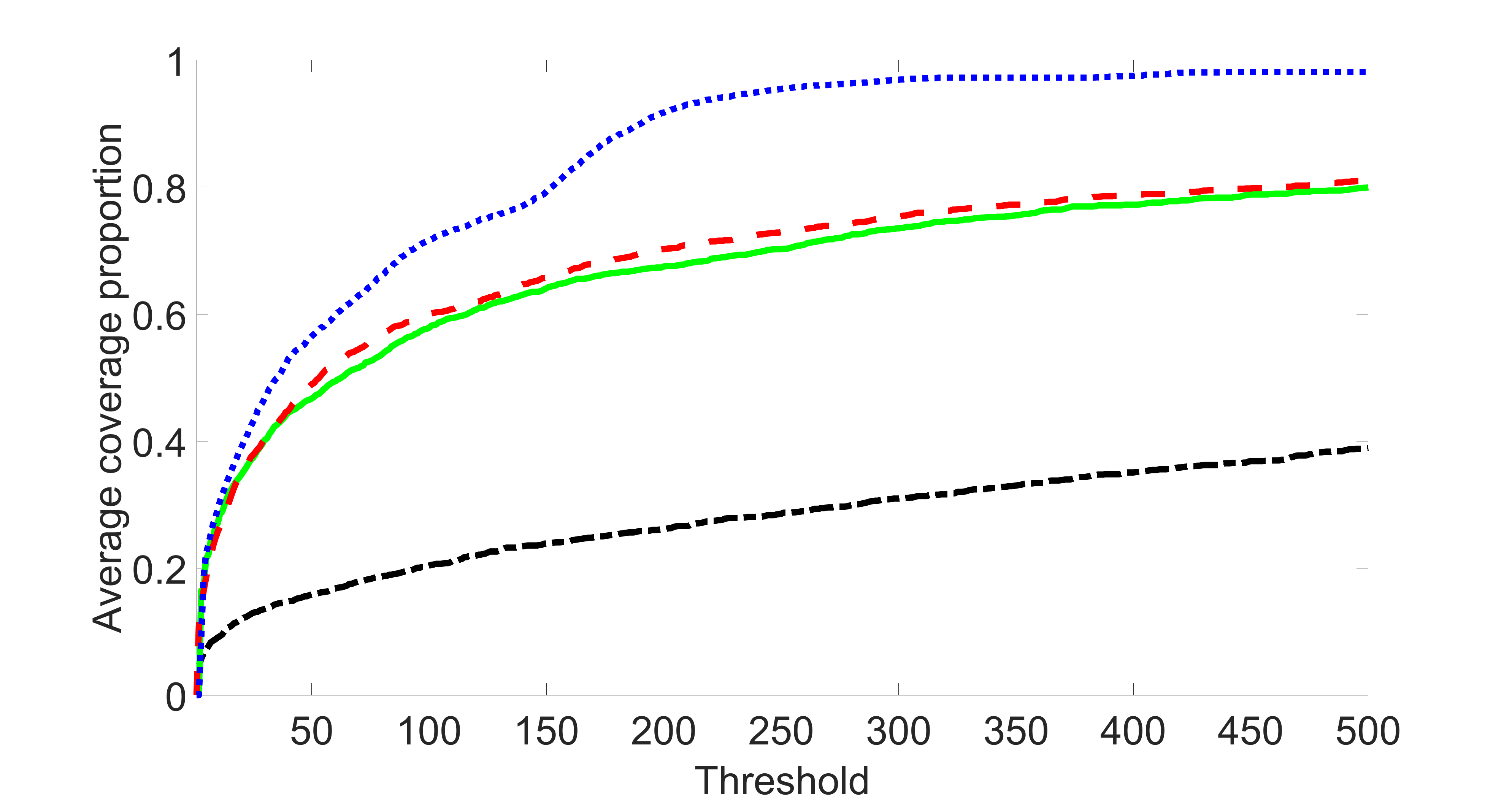
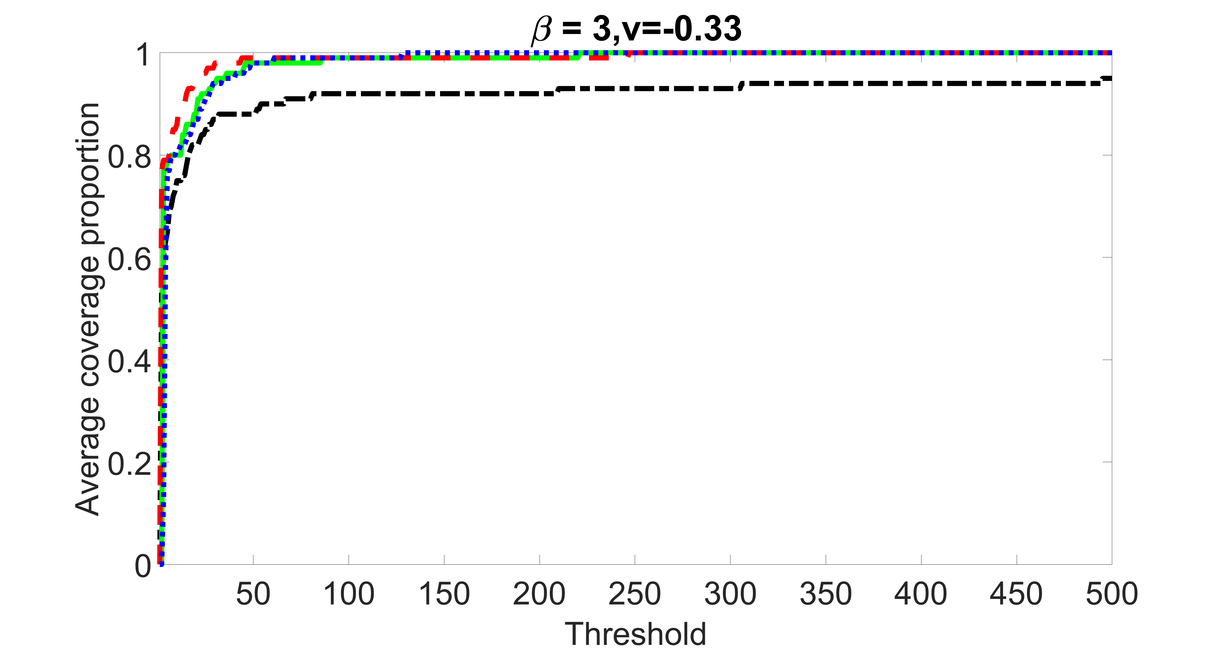
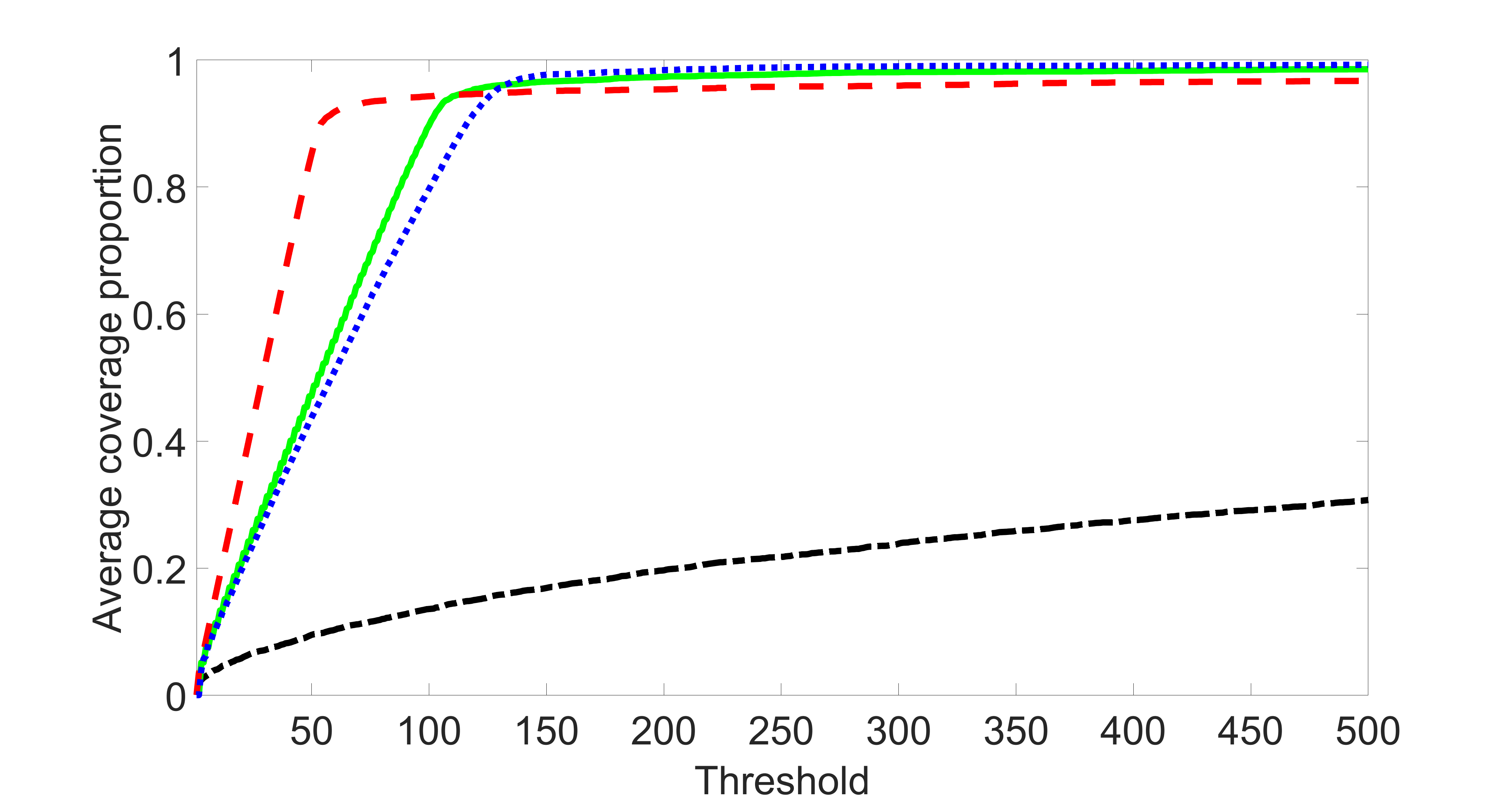
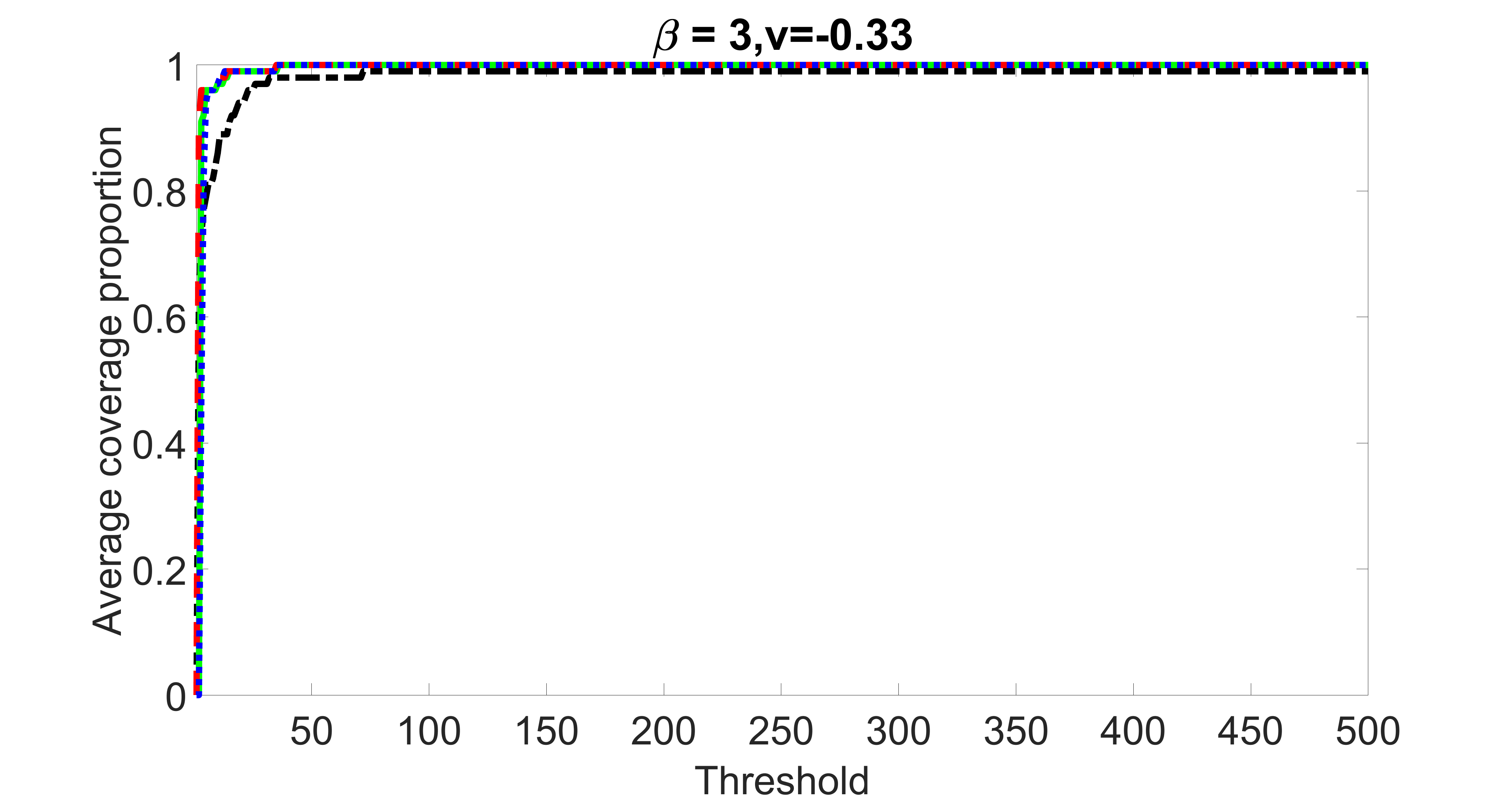
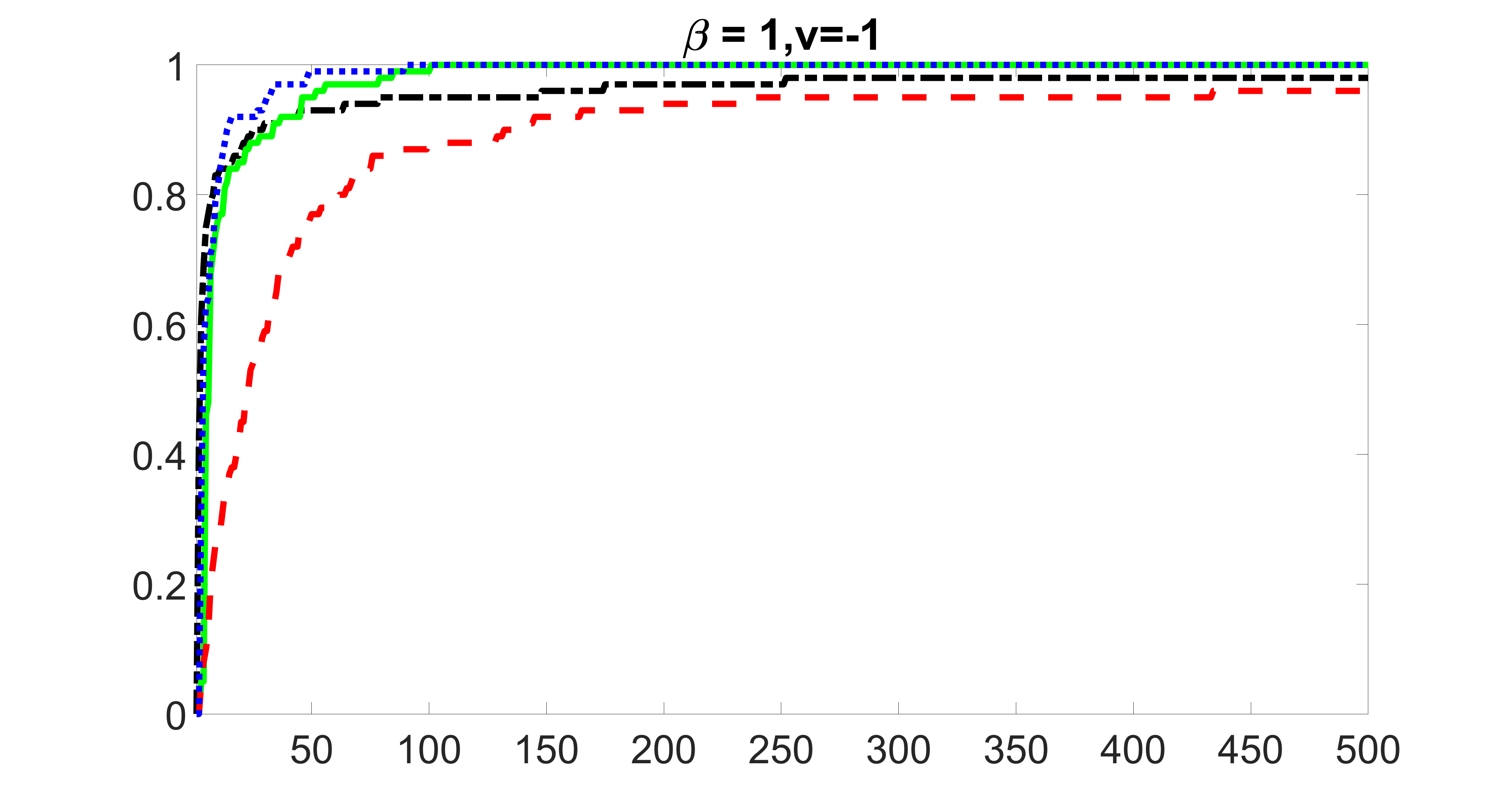
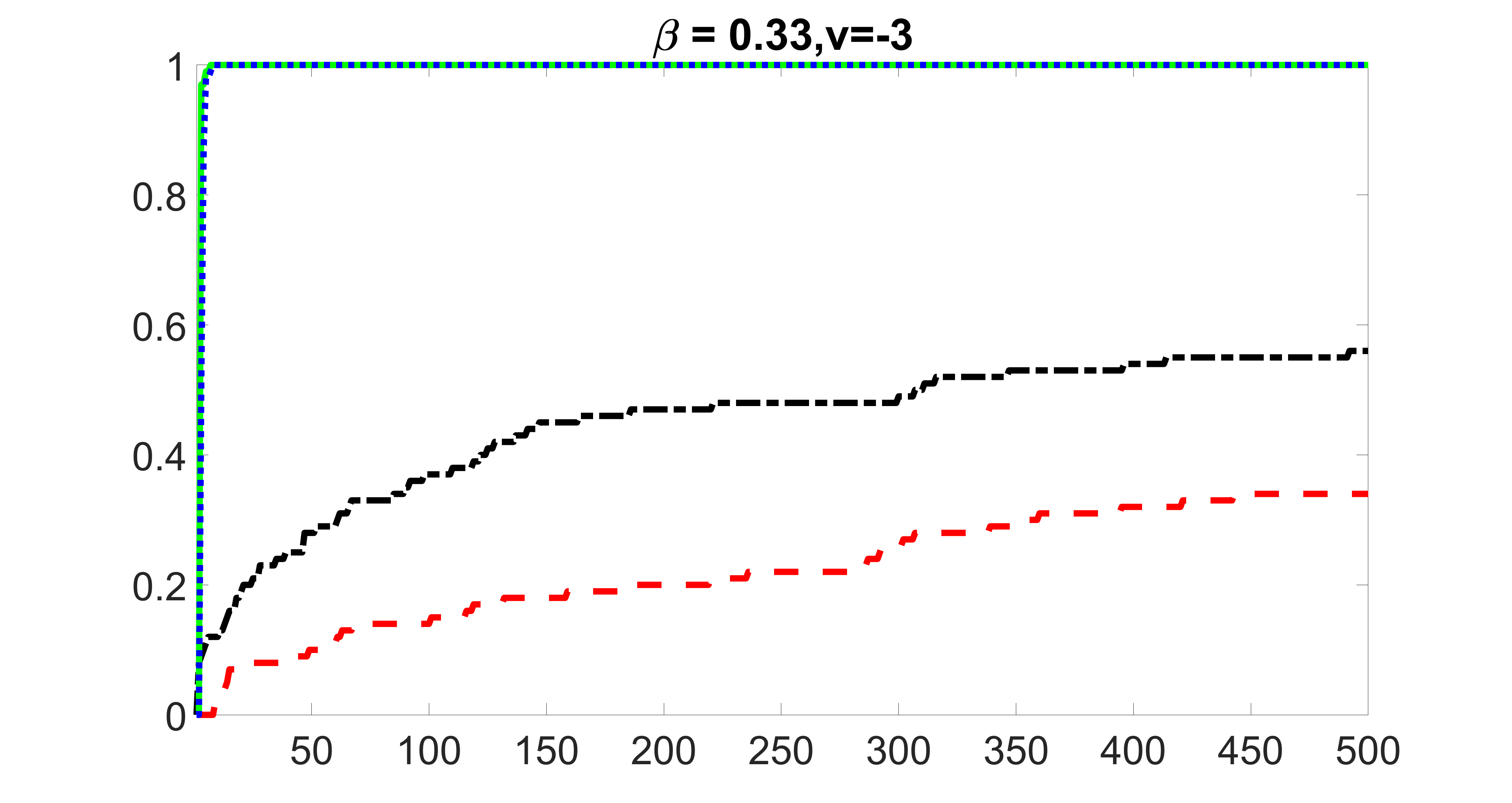
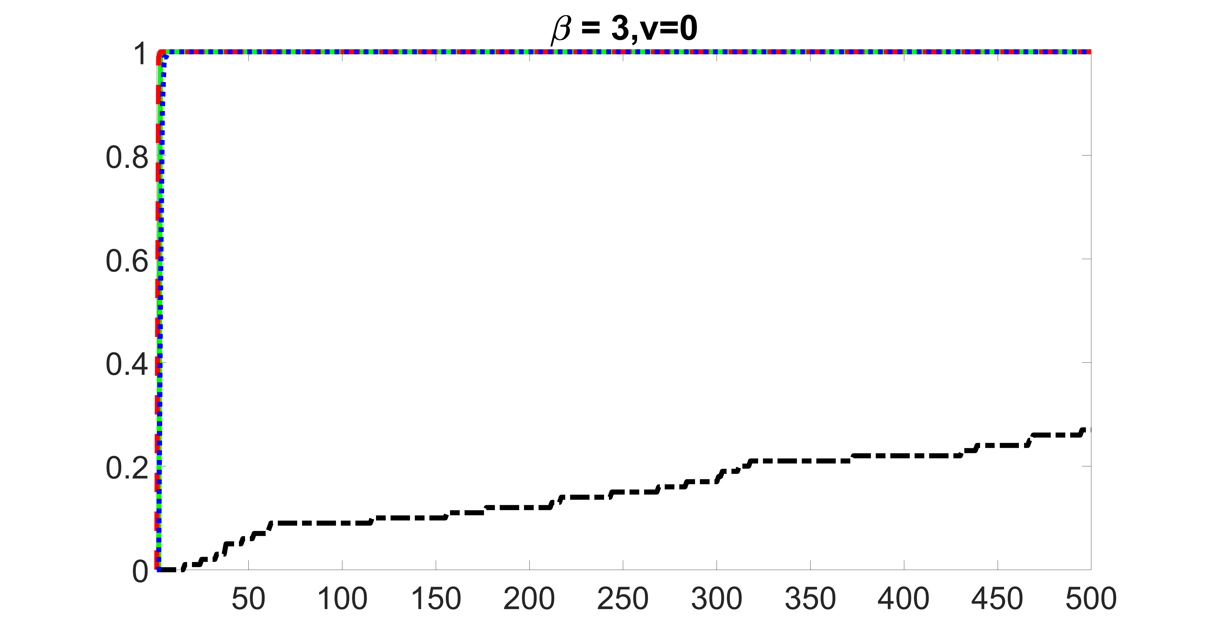
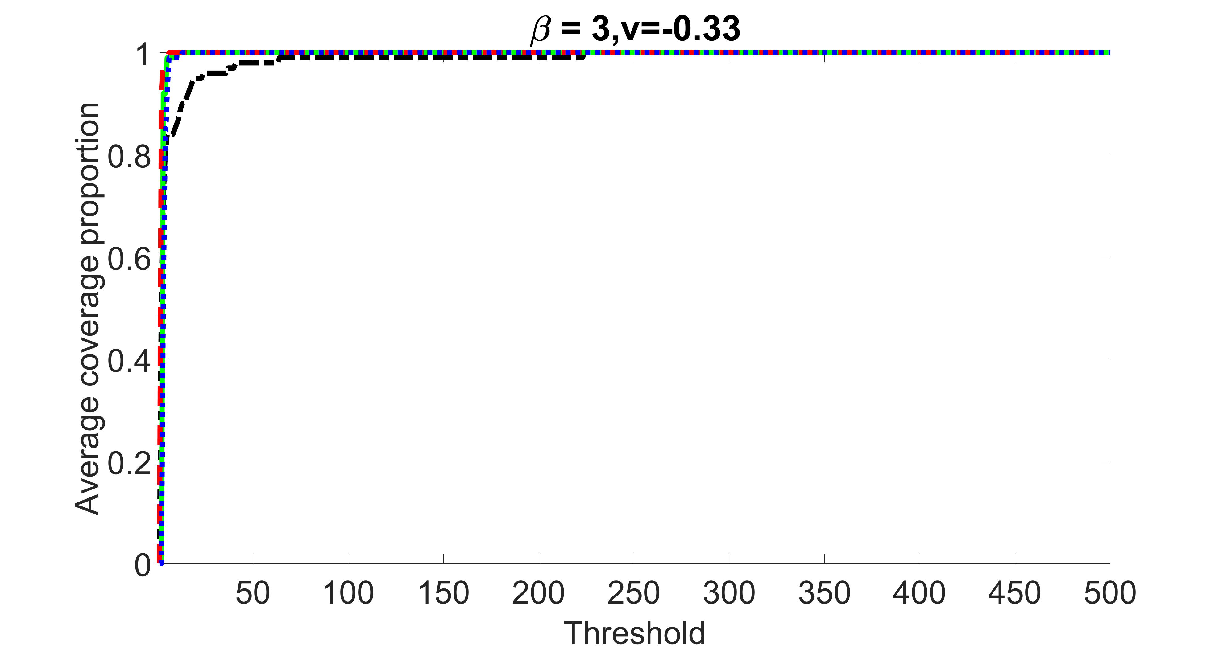
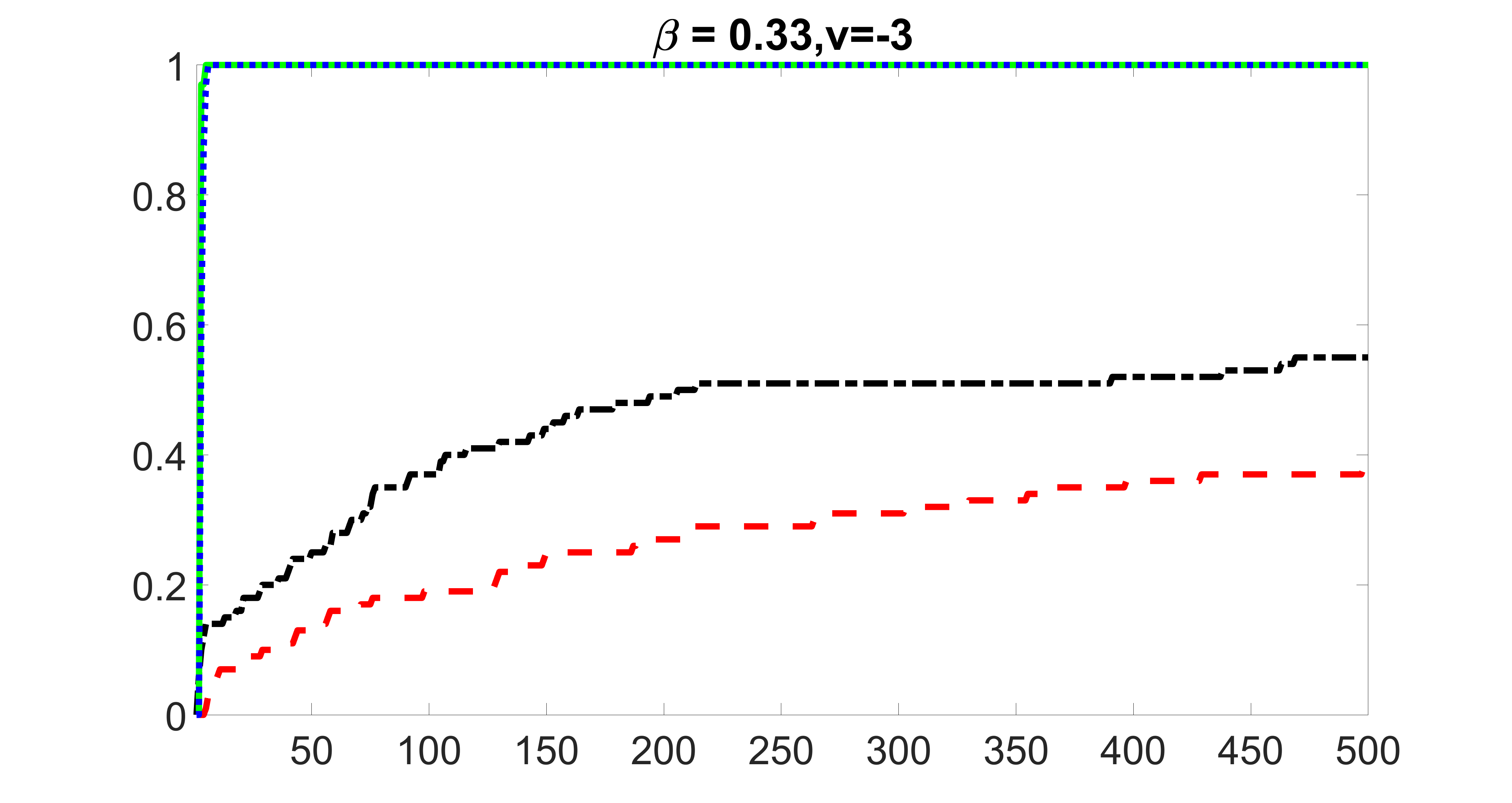
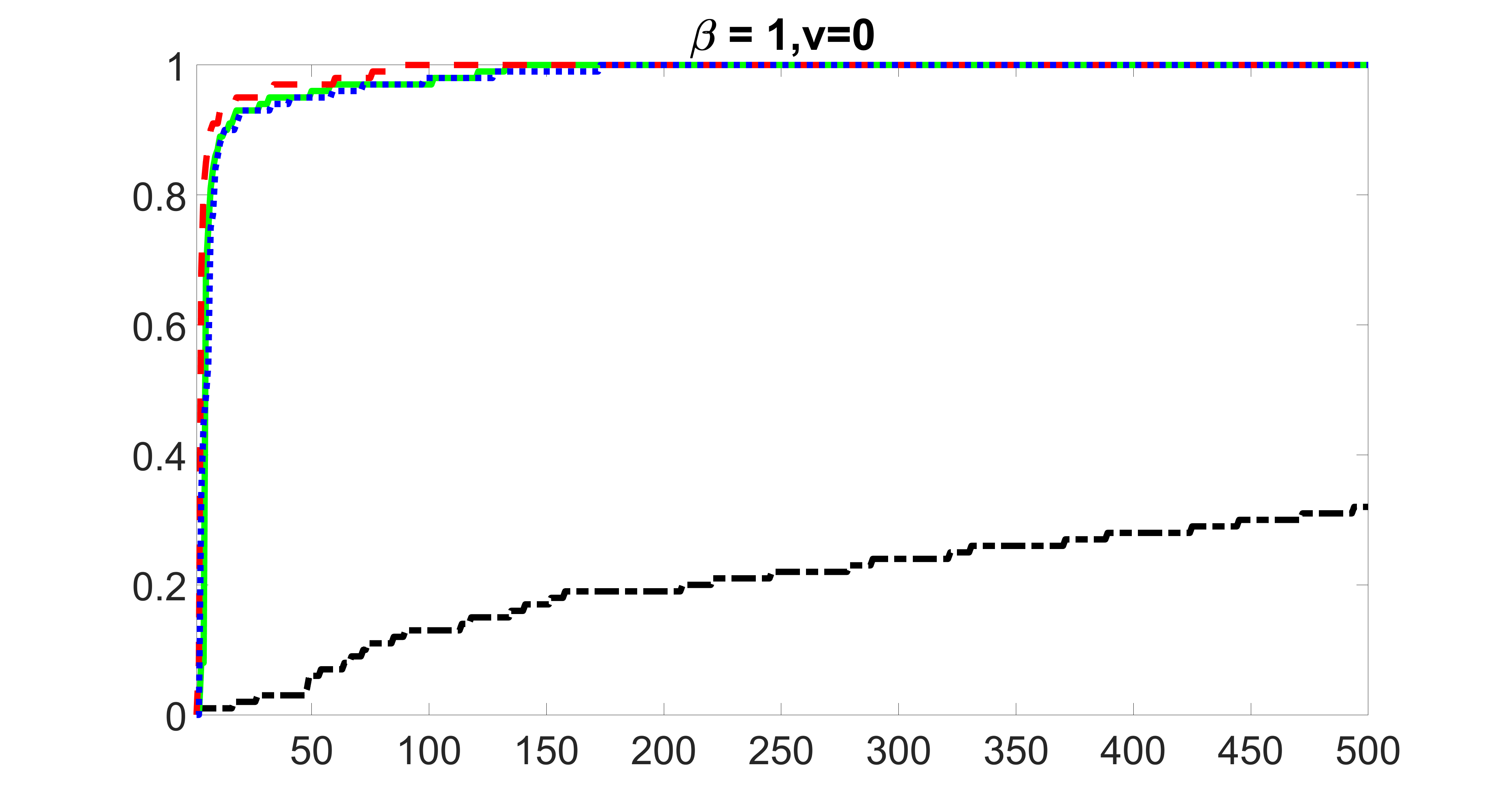
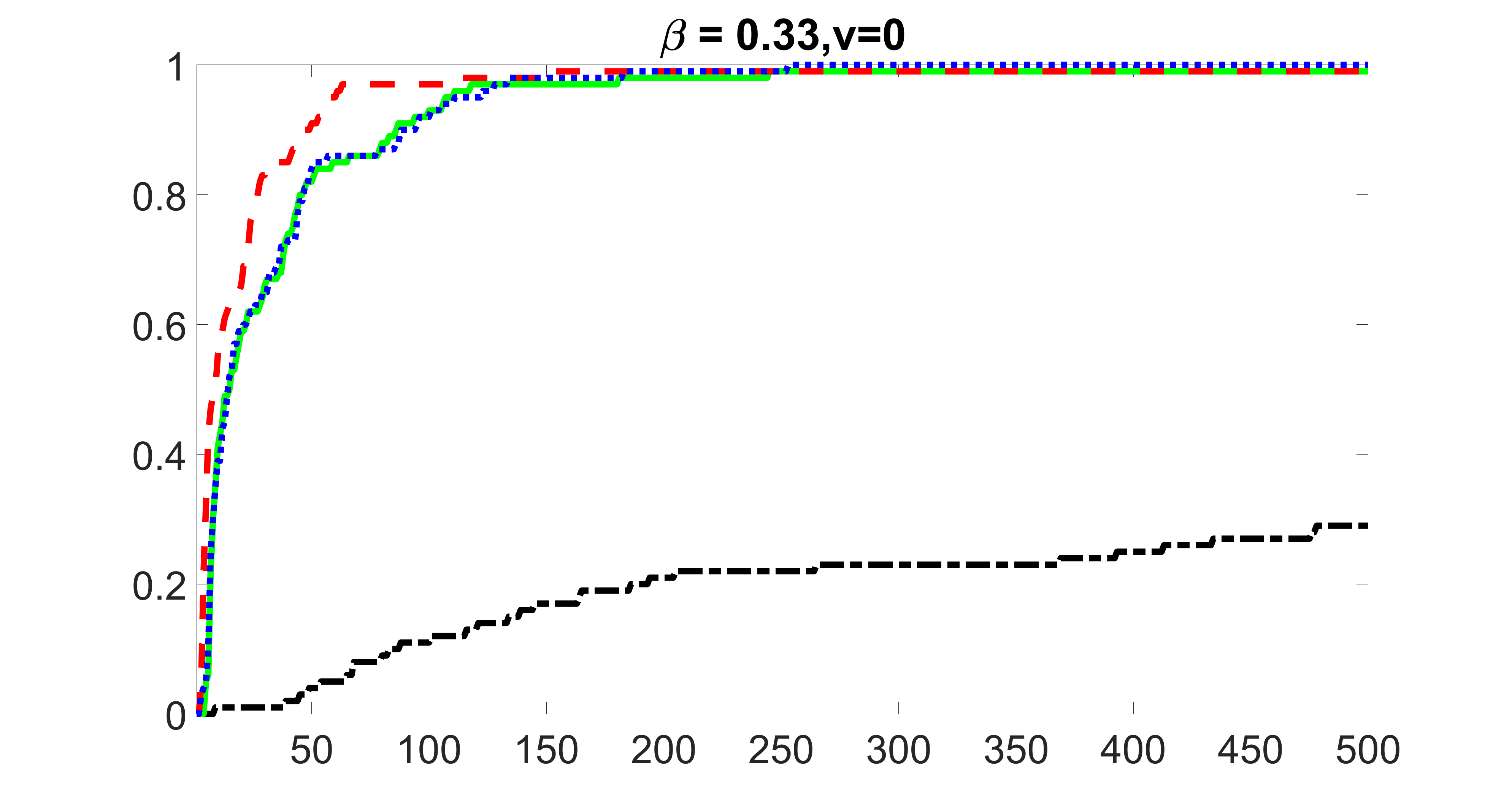
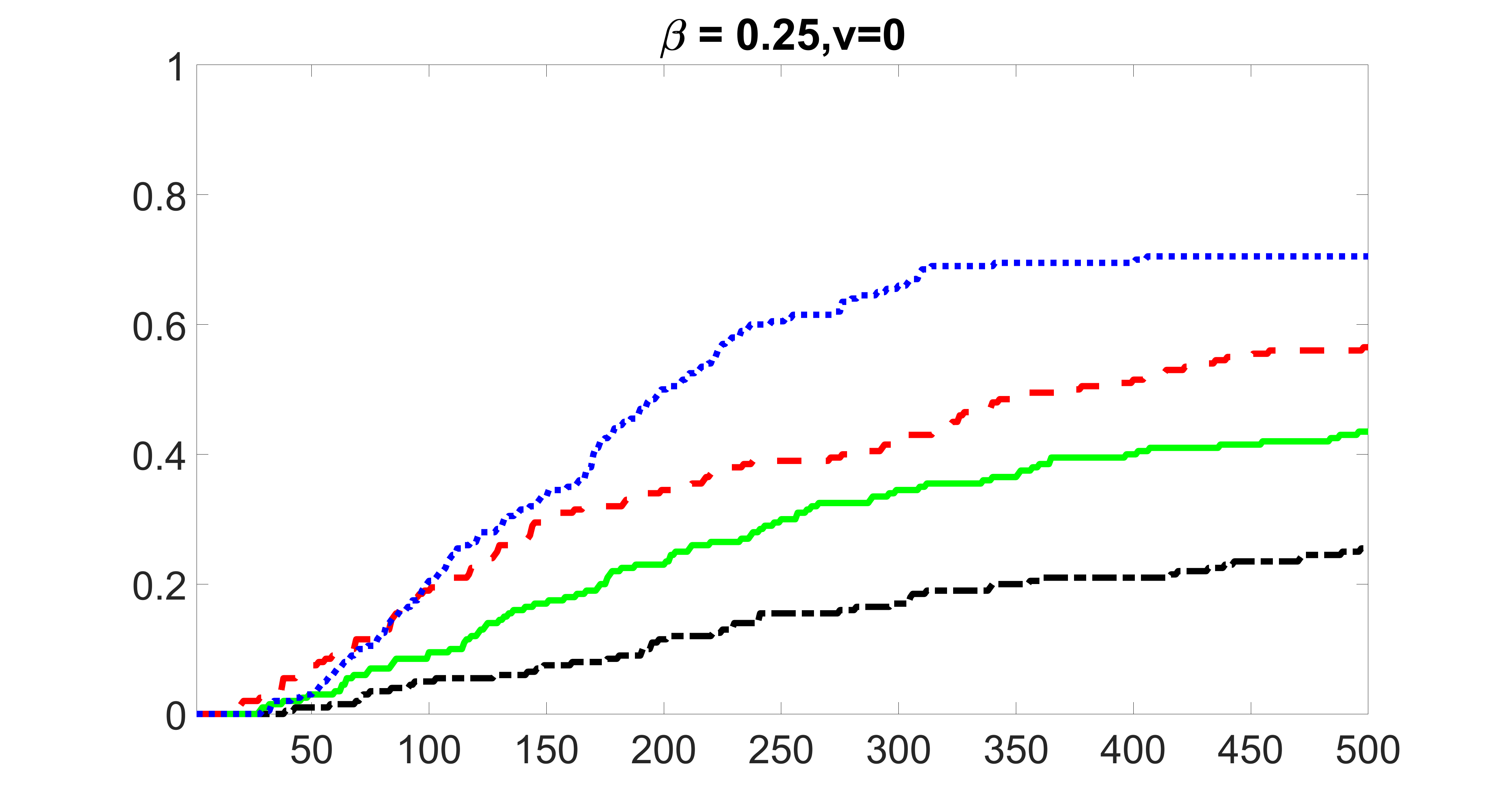
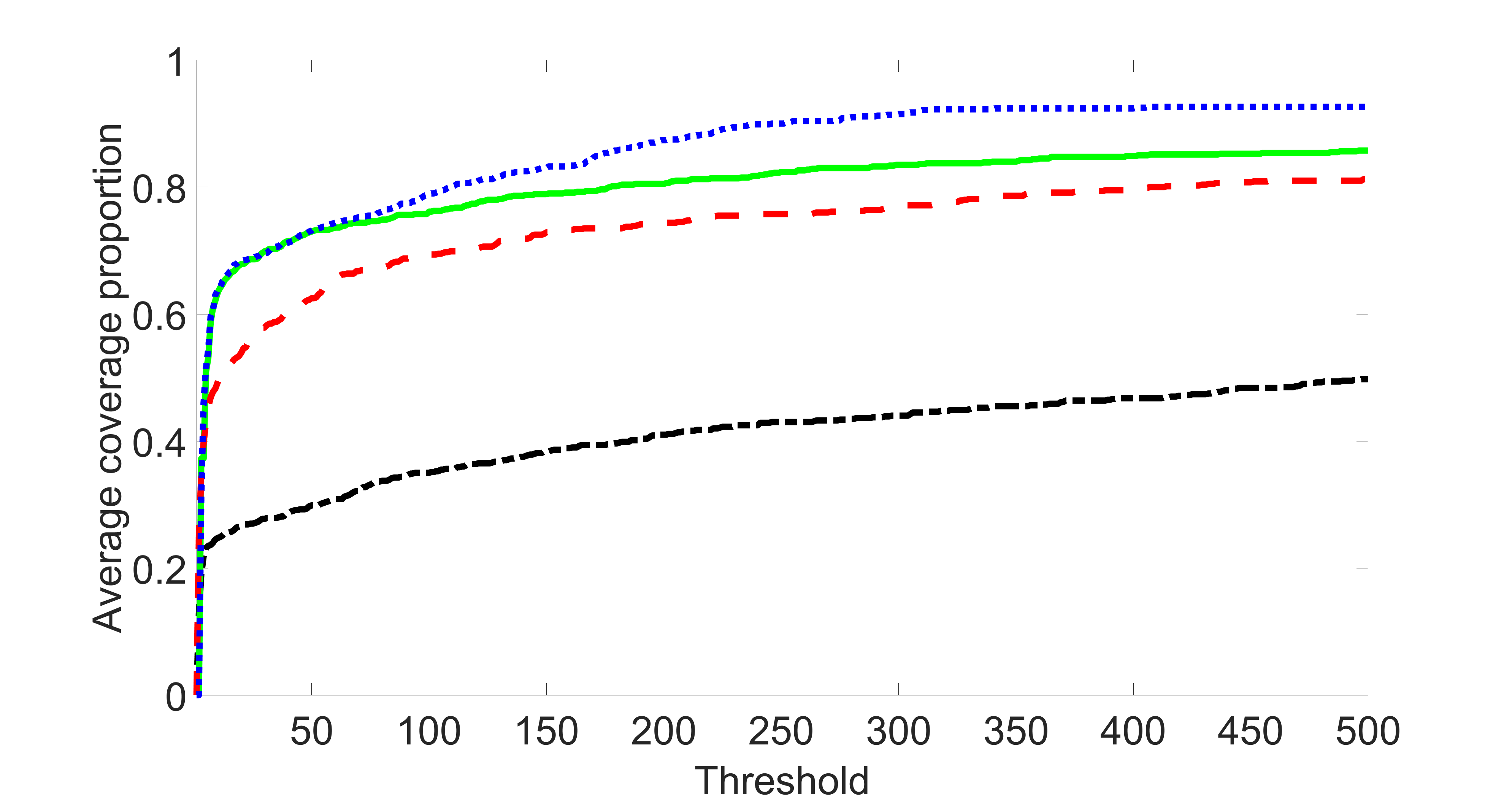
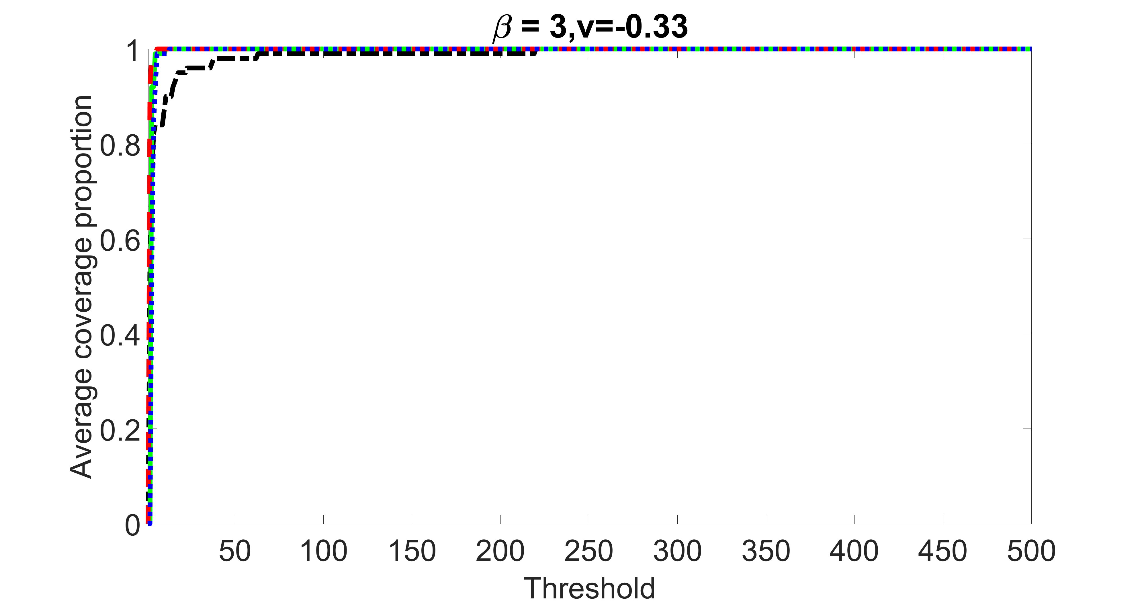
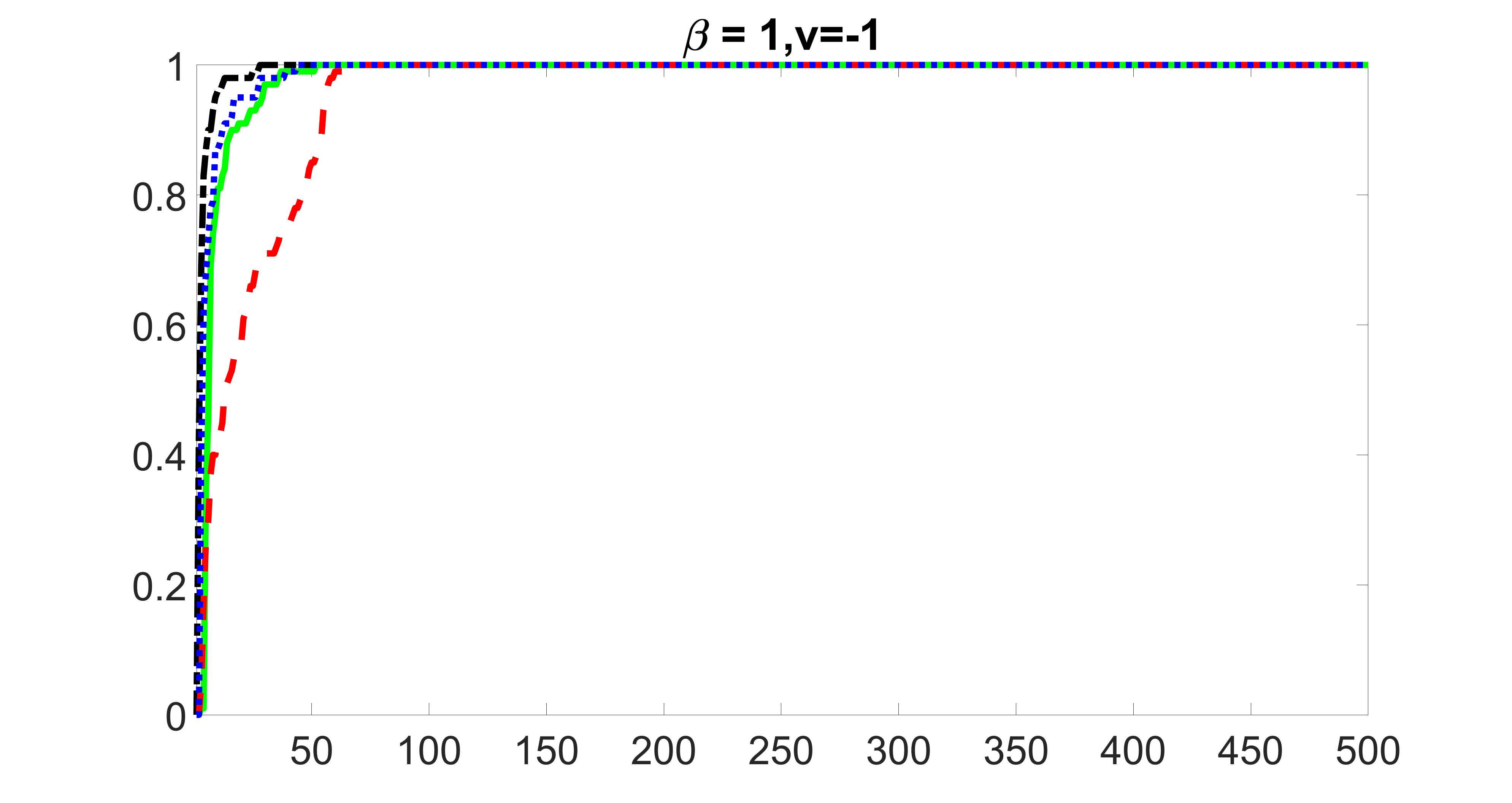
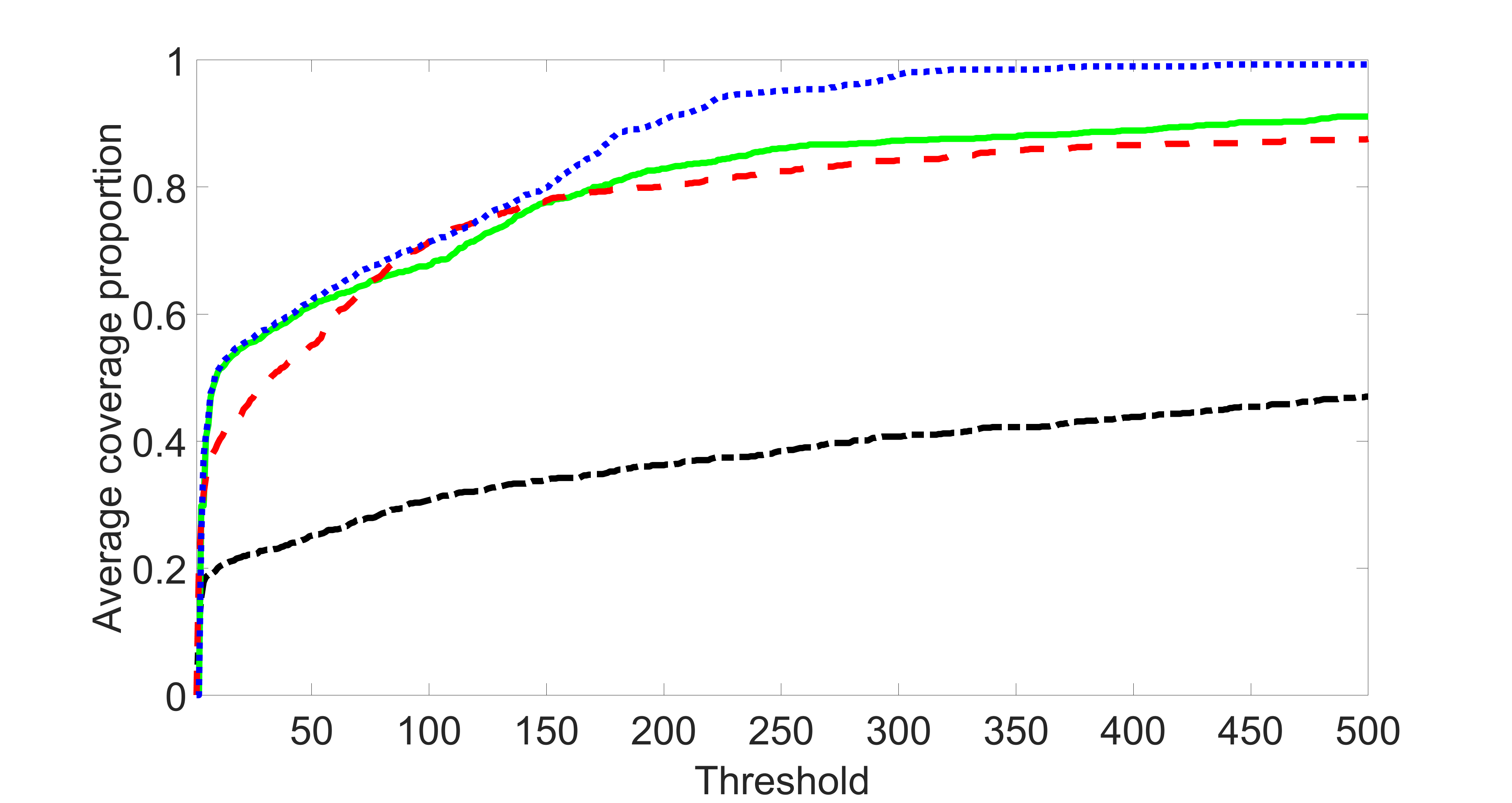
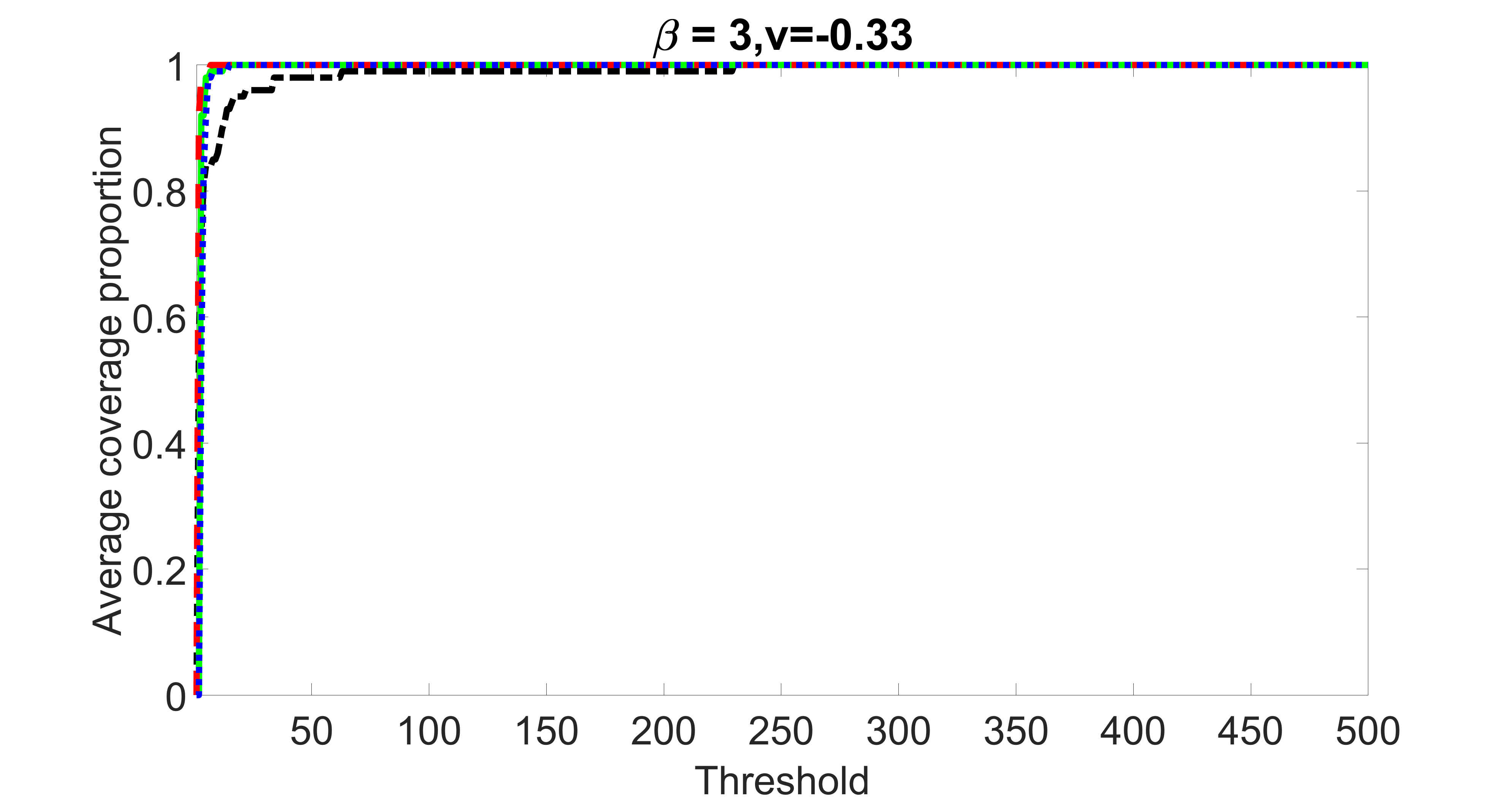
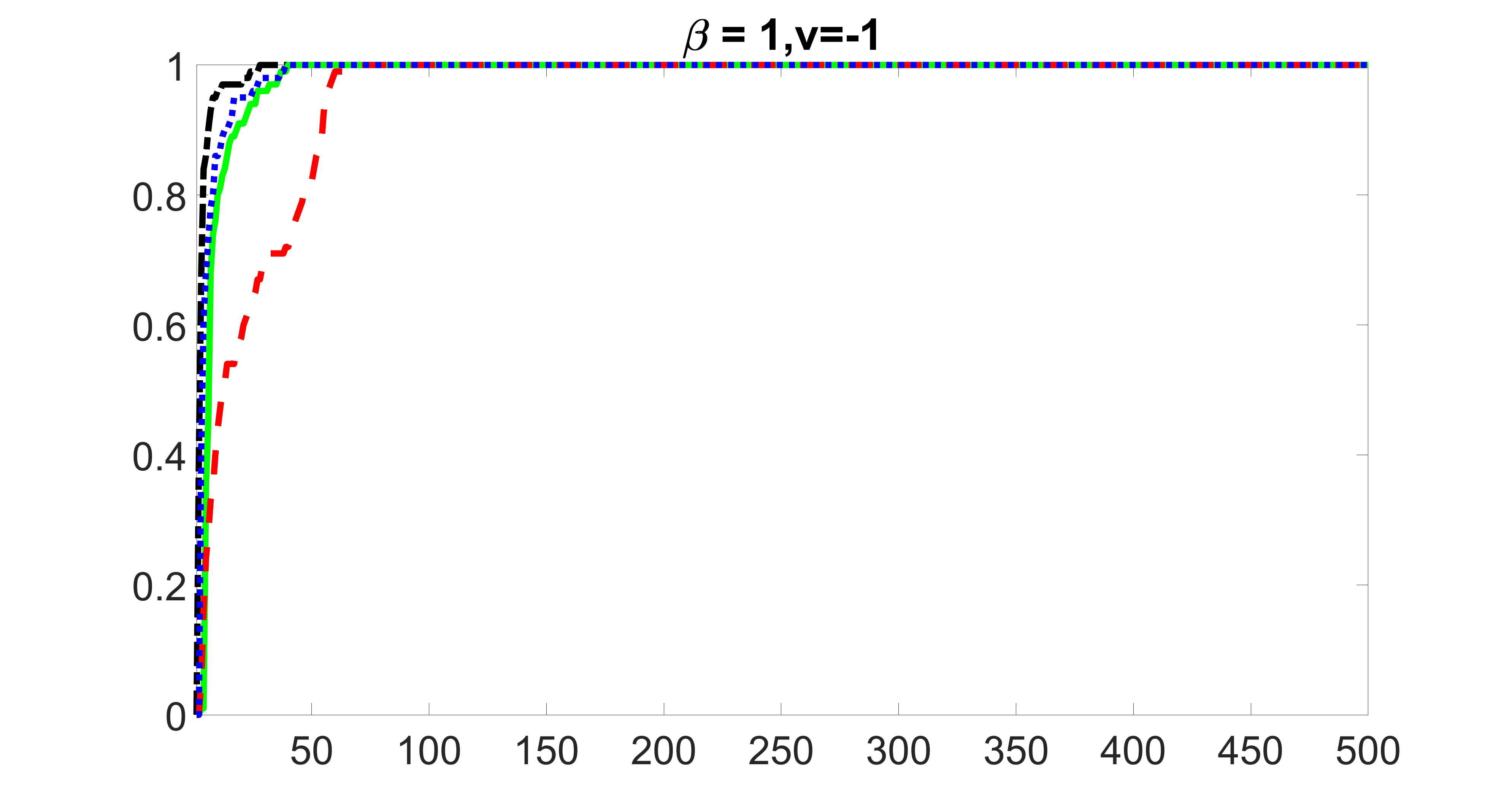
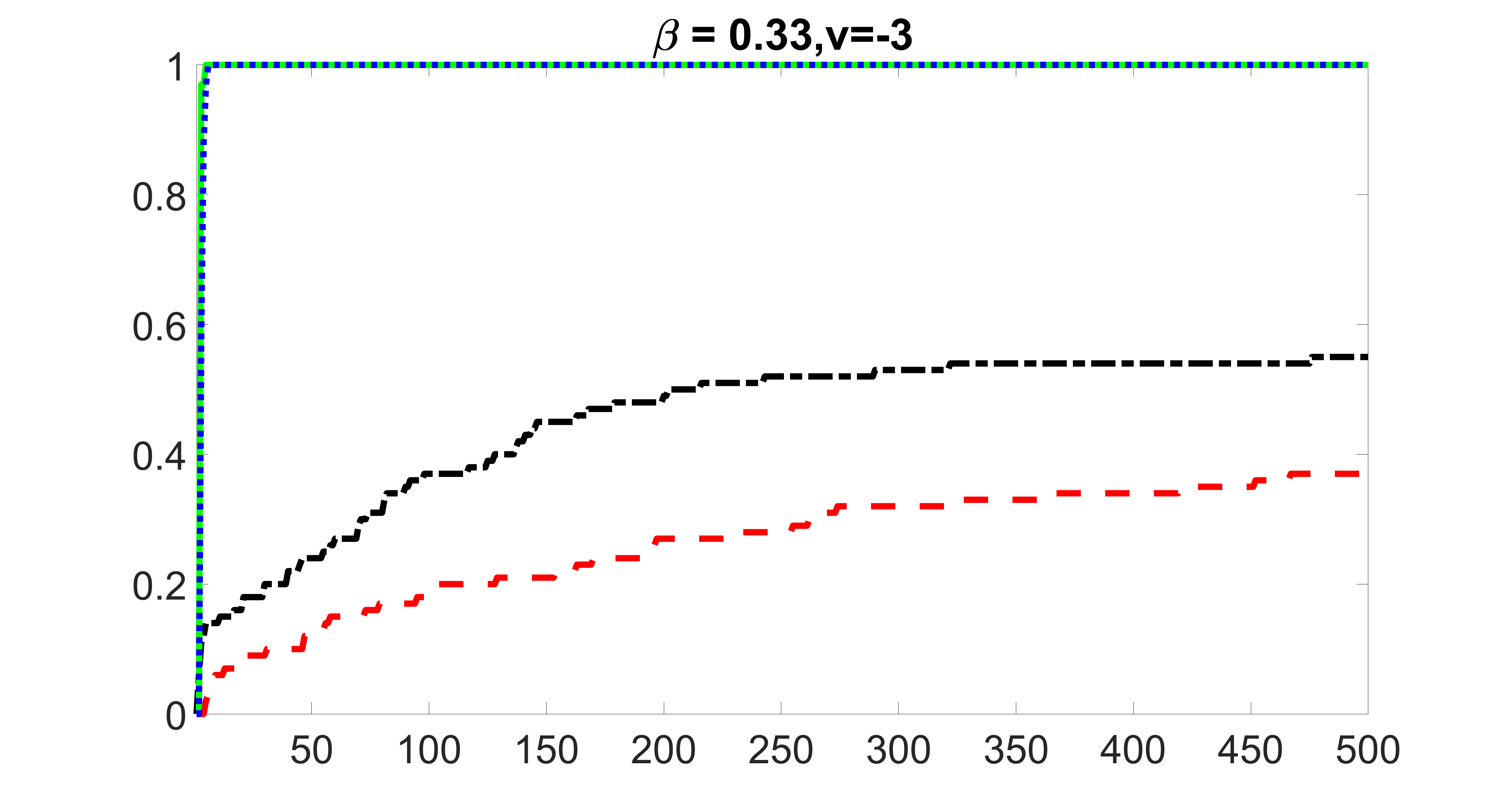
We perform our screening procedure (denoted by “joint”) and report the coverage proportion of , which is defined as , where the size of the selected set changes from to . In addition, we report the coverage proportion for each of the confounding and precision variables, i.e. each of the ’s in the set . All the coverage proportions are averaged over Monte Carlo runs.
To control the changing size of the , we first set by specifying appropriate and . Then we sequentially add two variables, one to by increasing and one to by increasing , until reaches . Note that we always keep in the procedure. We may not obtain all the sizes between and because may increase by at most . Therefore, for those sizes that cannot be reached, we use a linear interpolation to estimate the coverage proportion of by using the closest two end points.
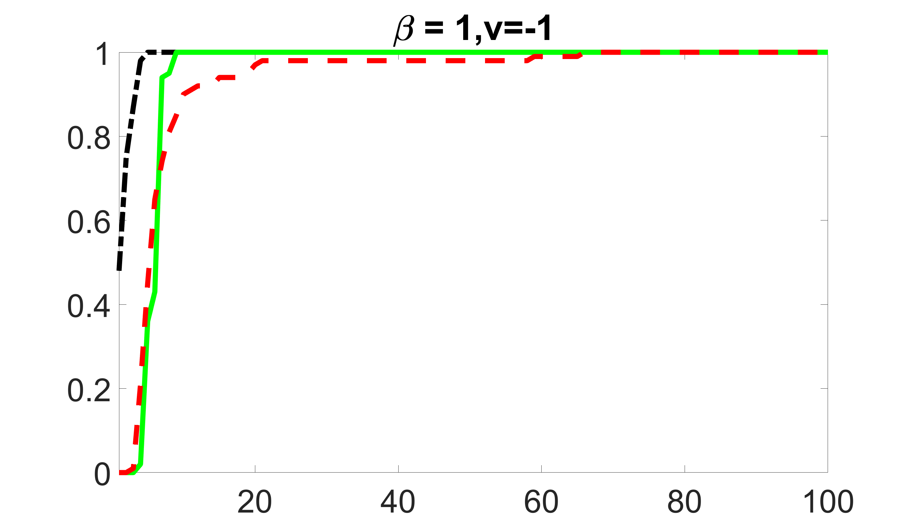
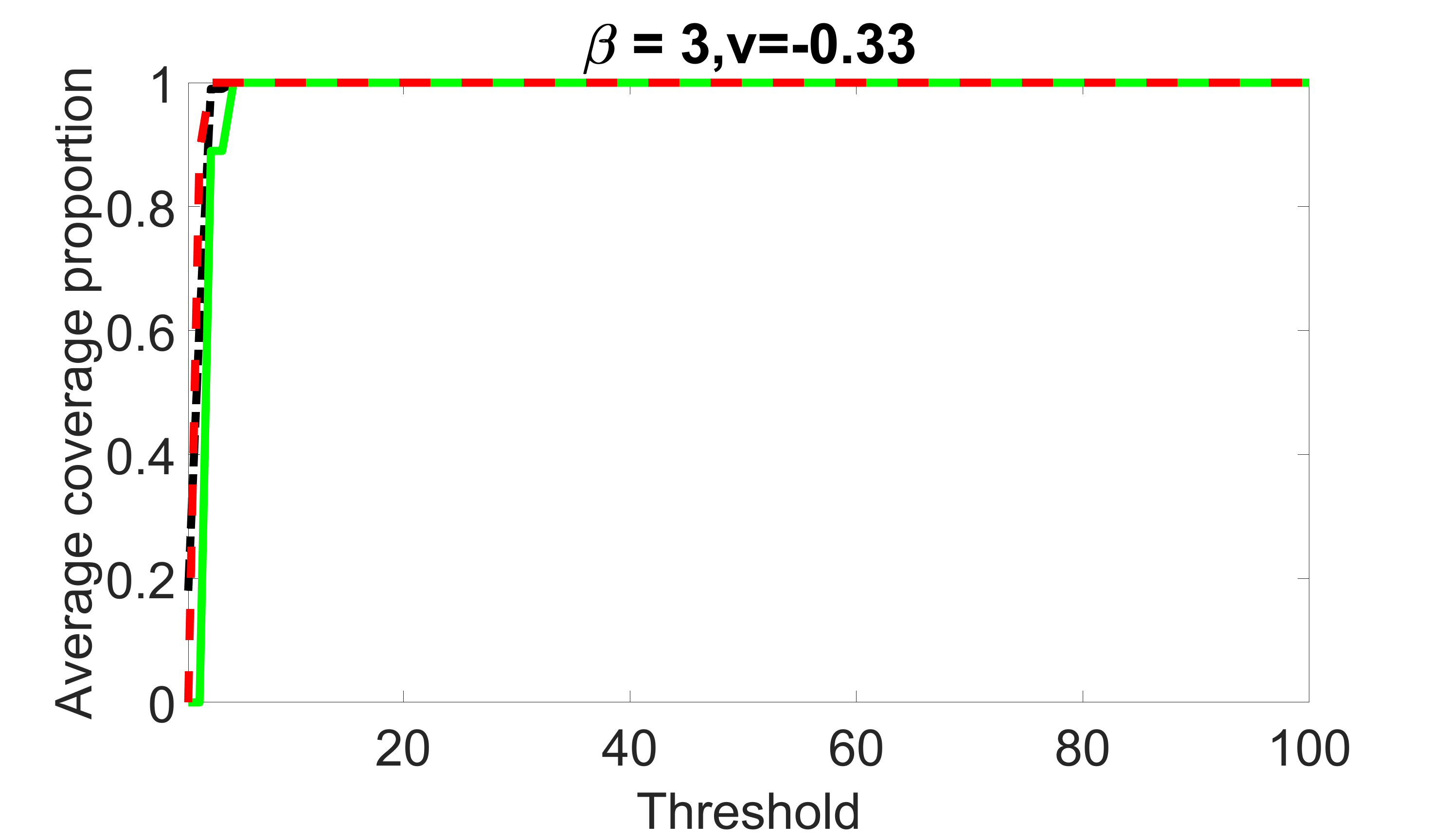
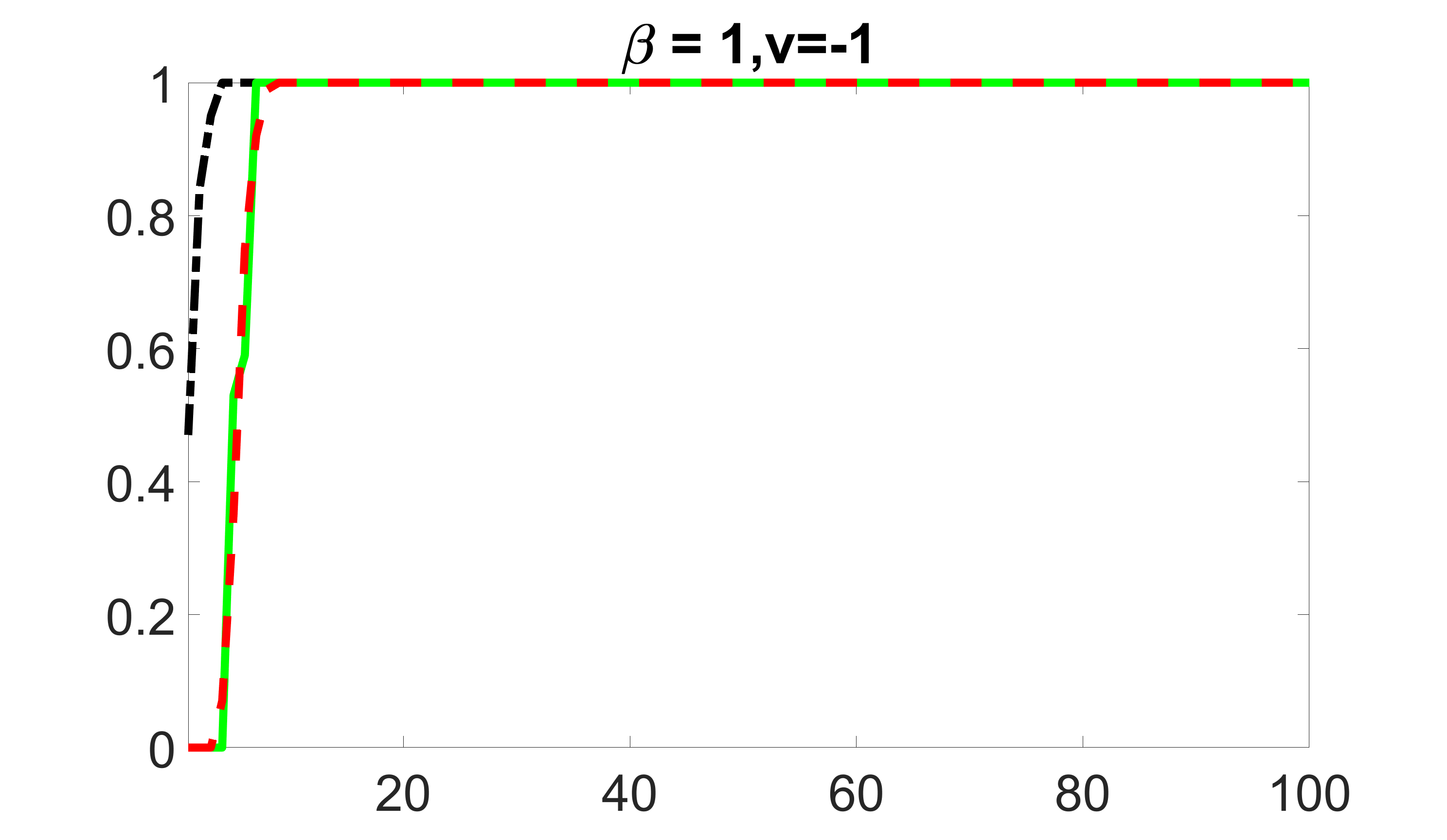
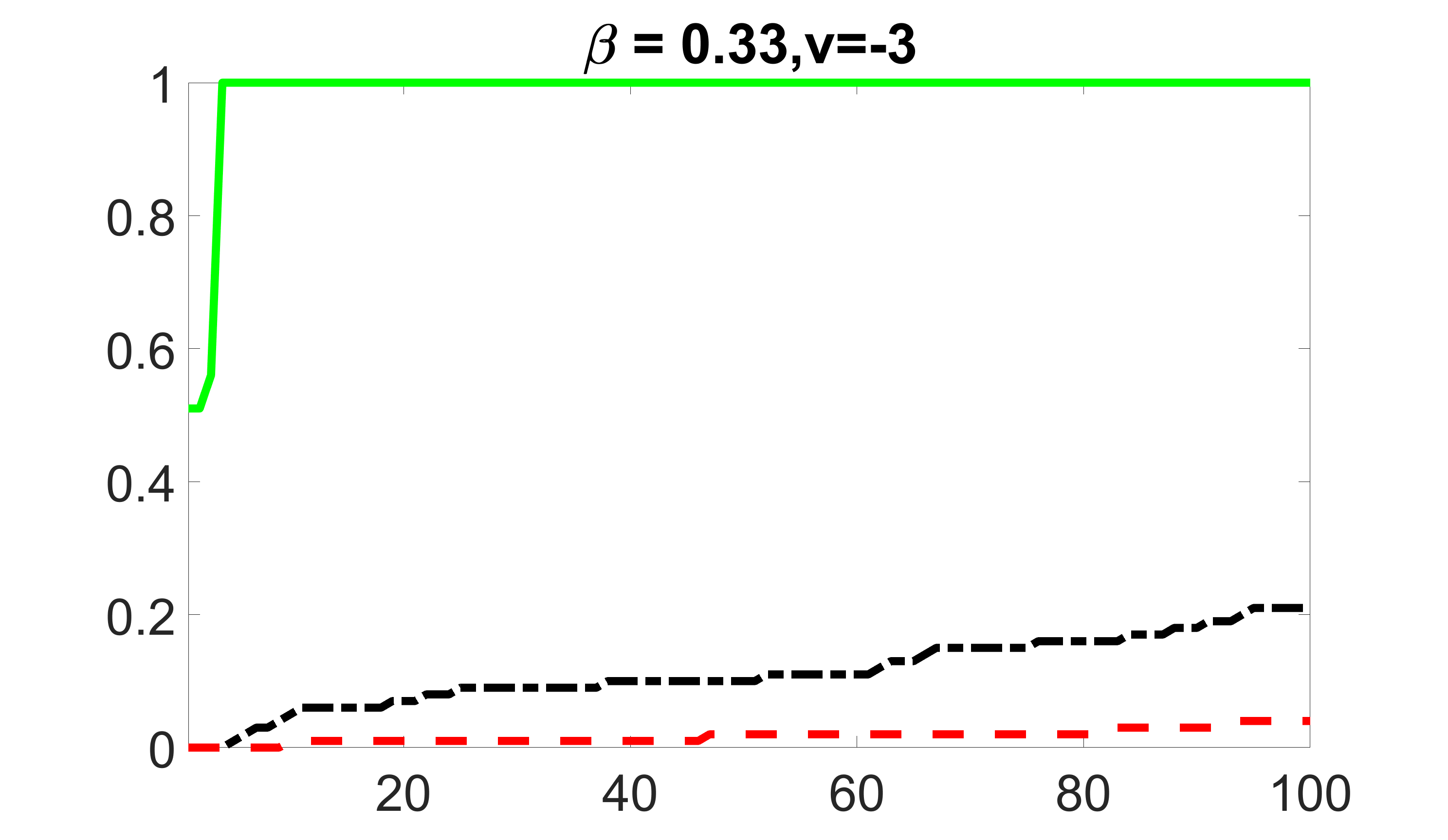
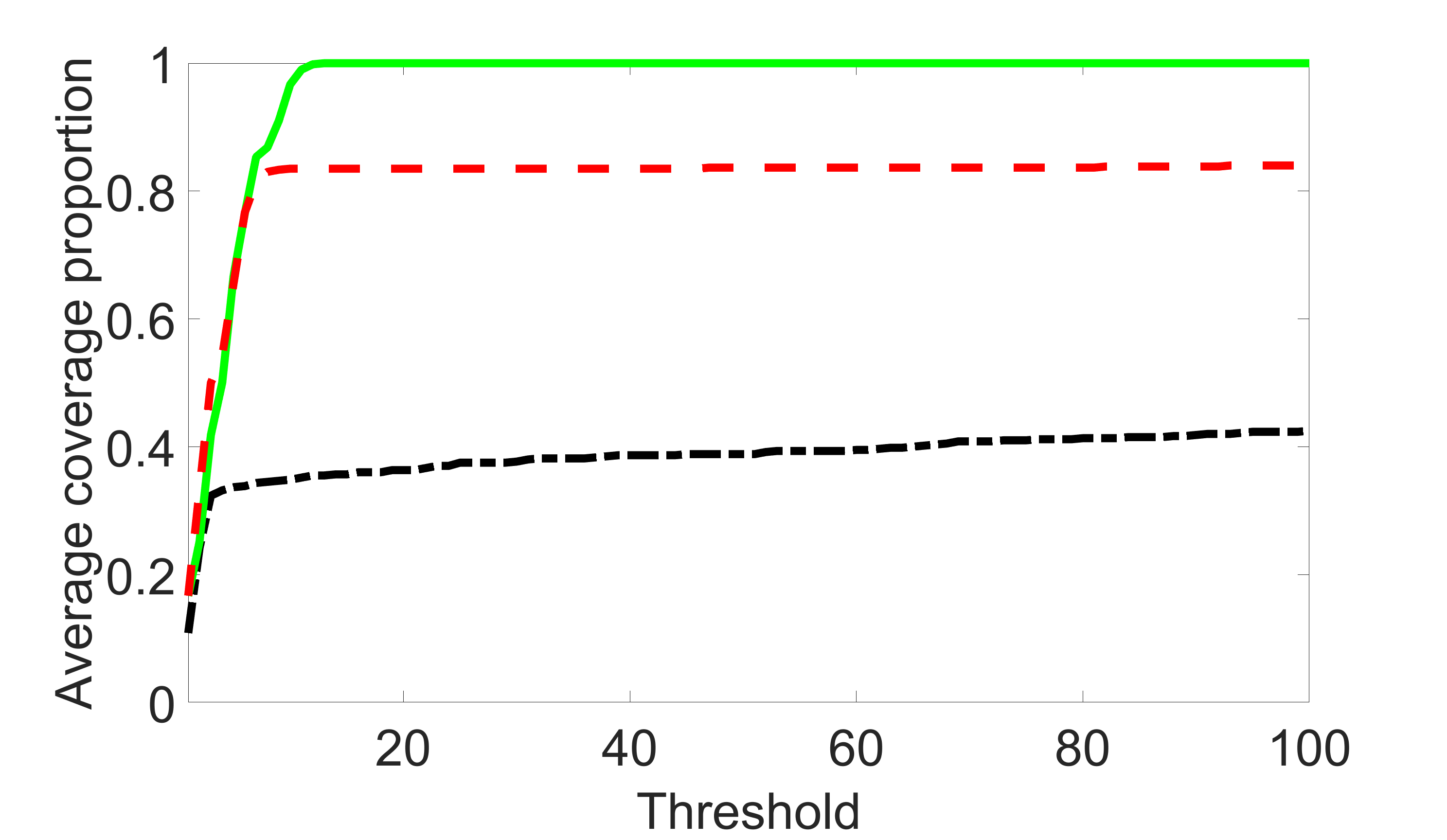
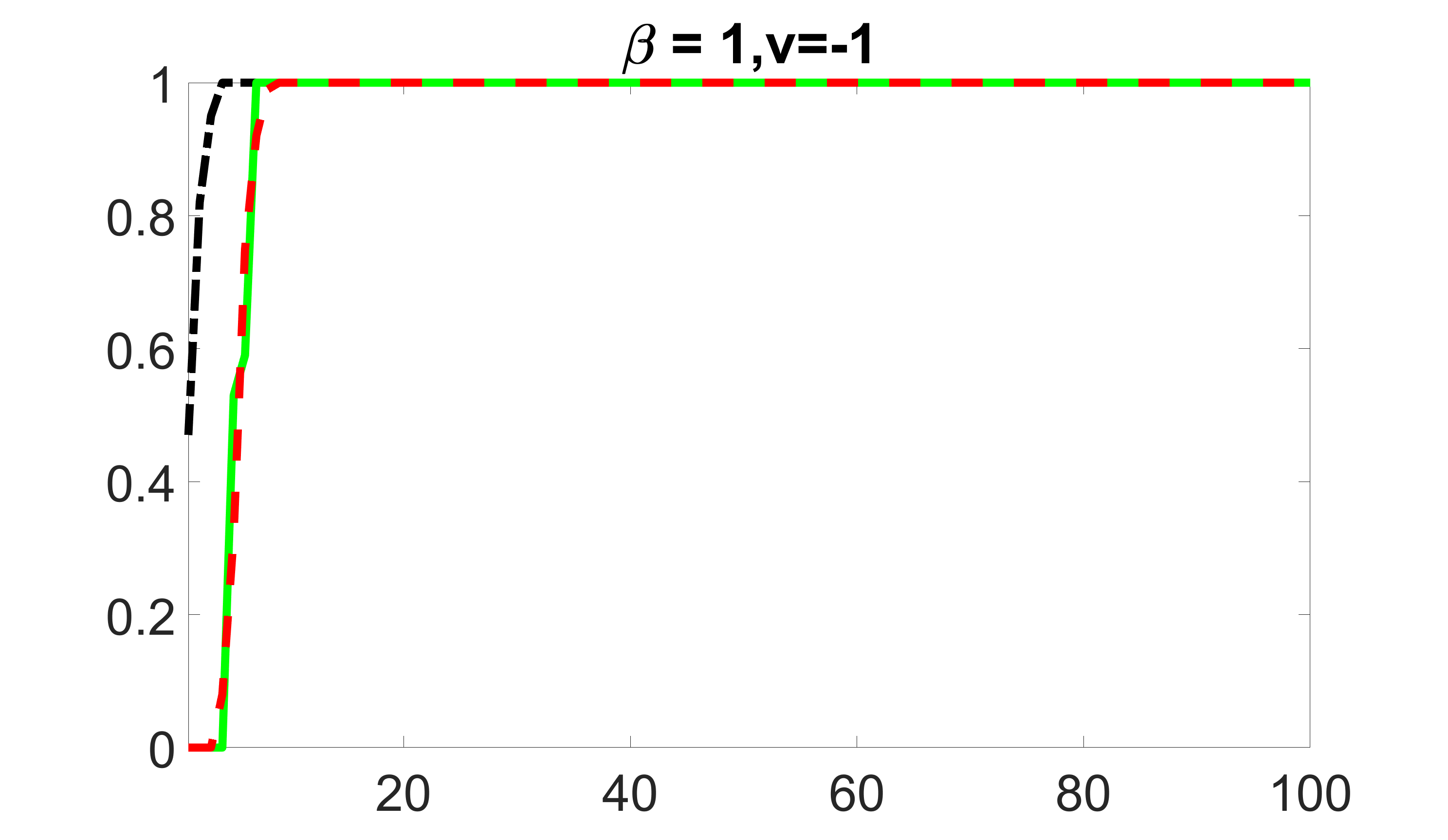
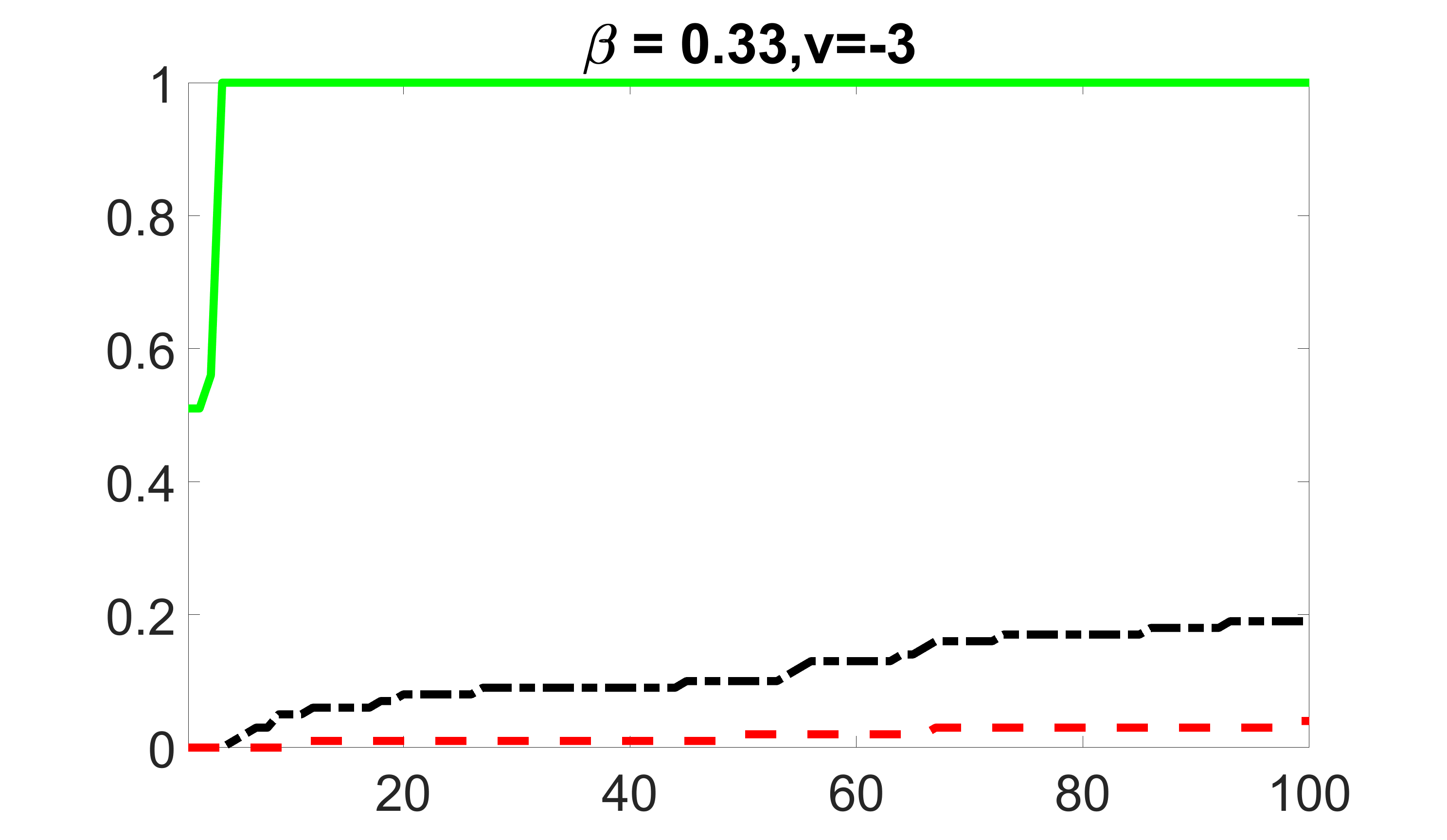
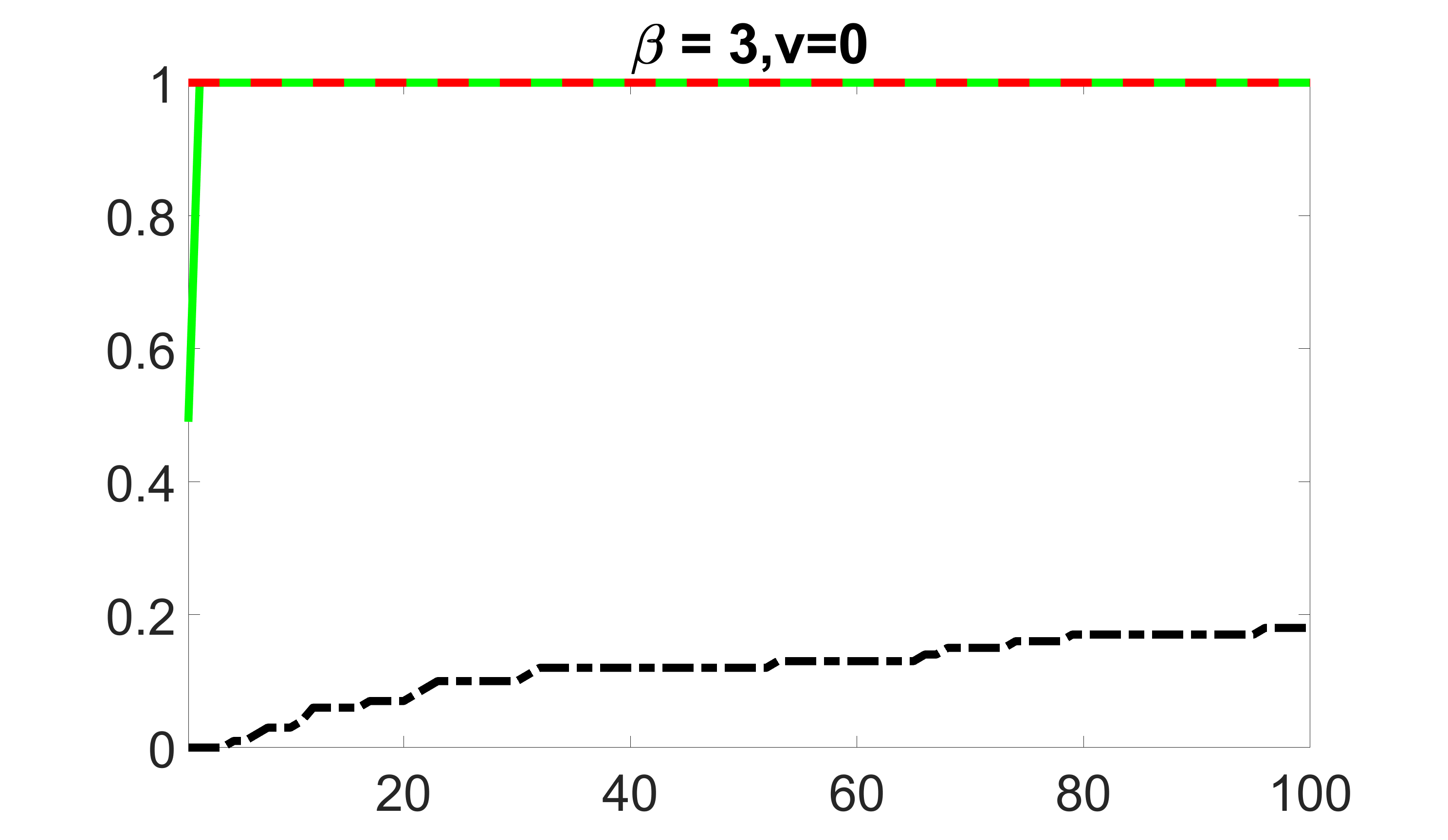
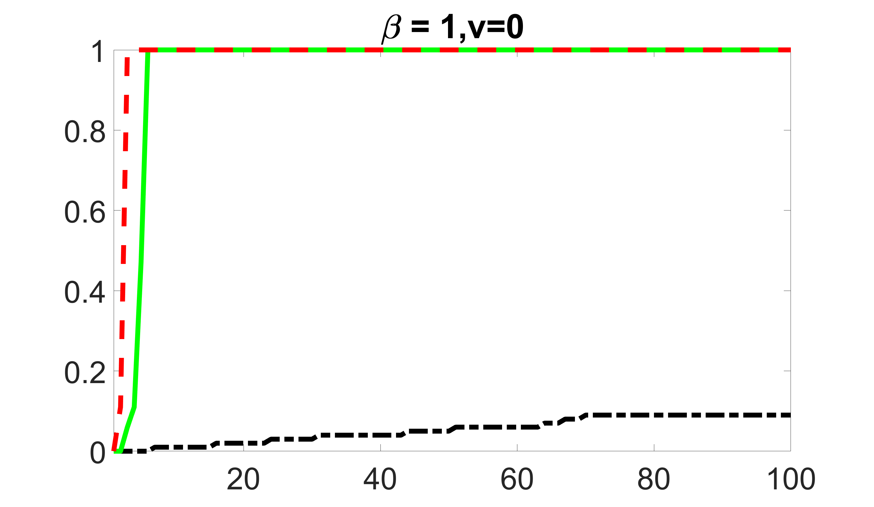
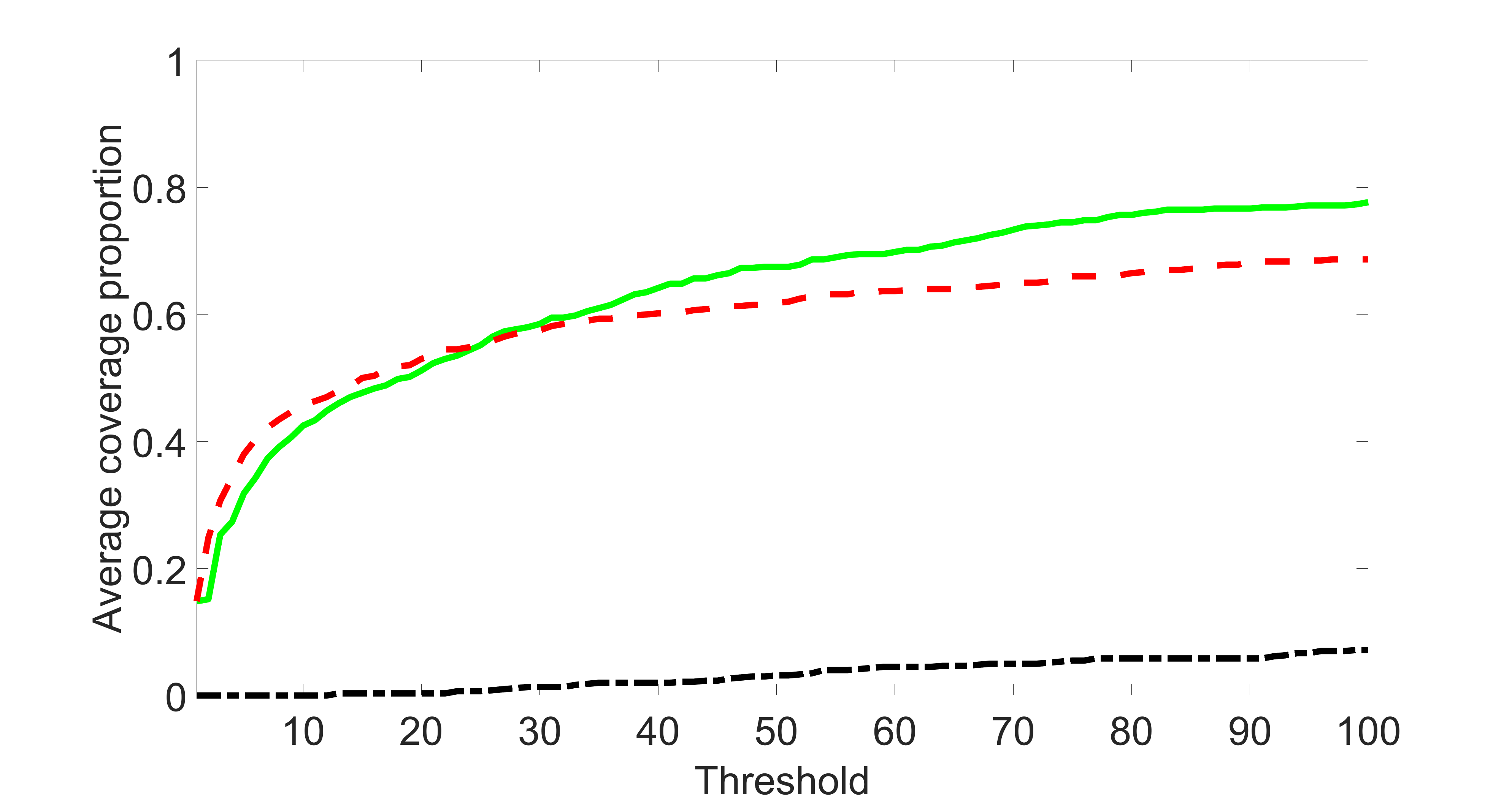
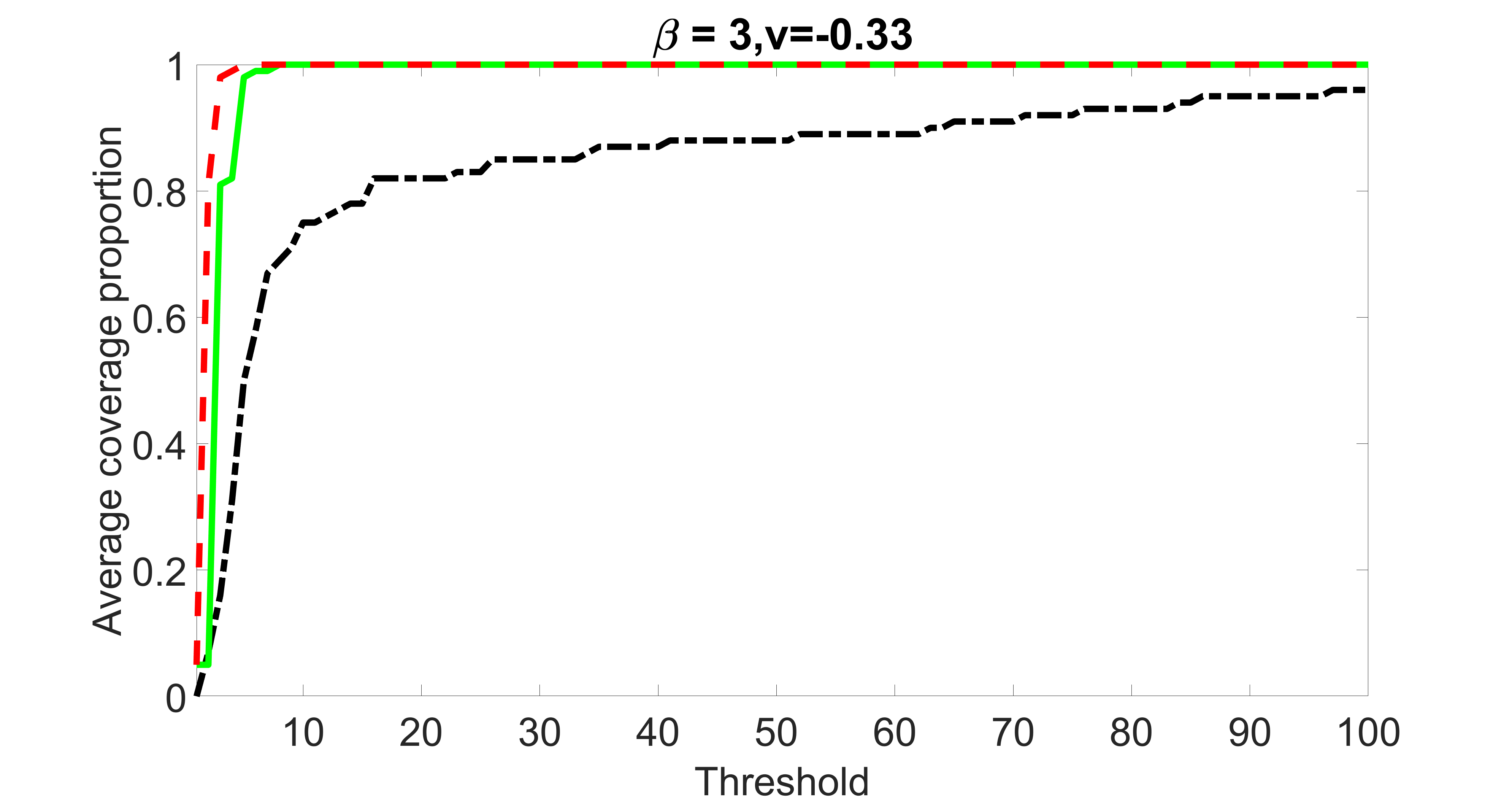
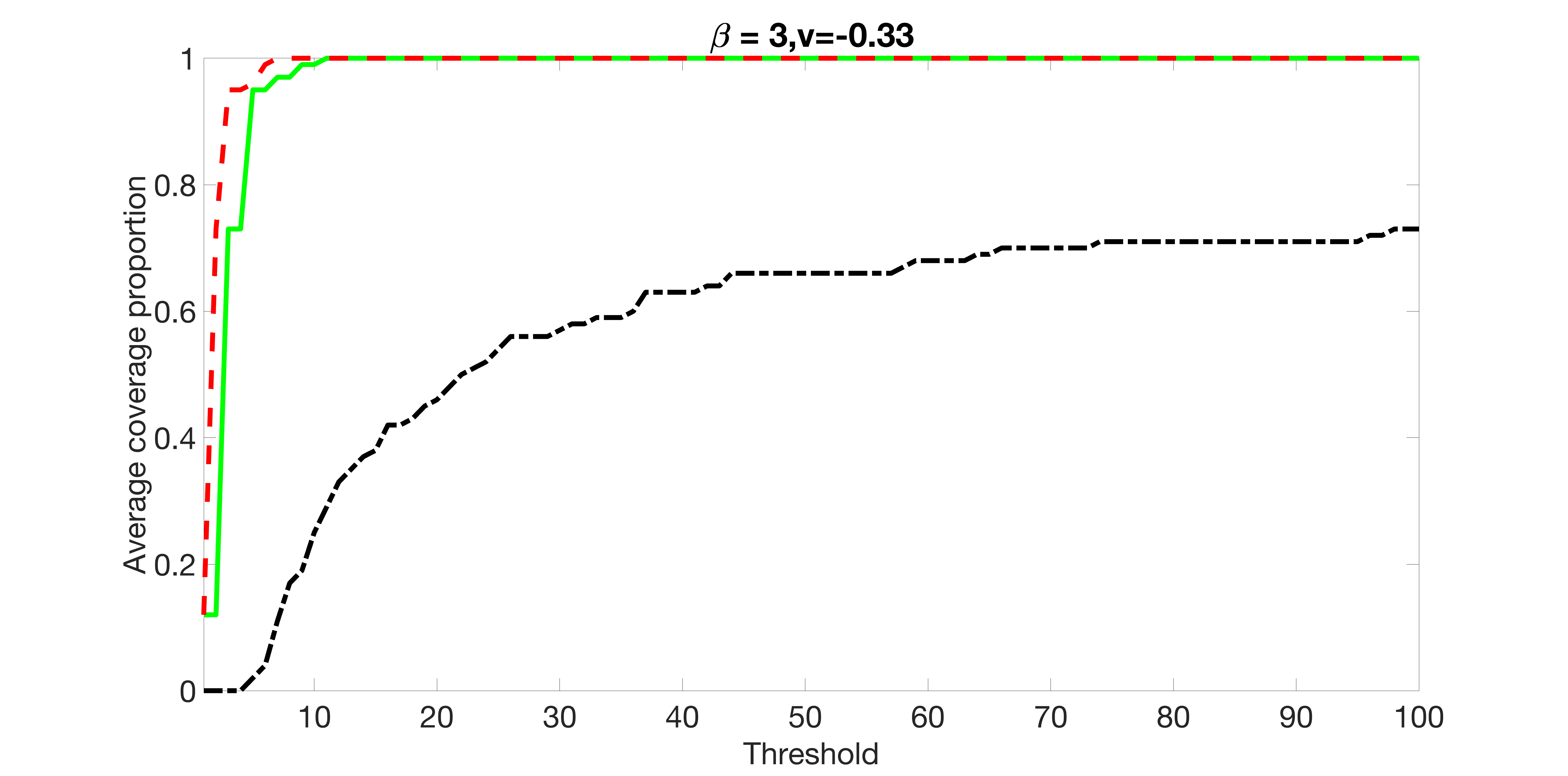
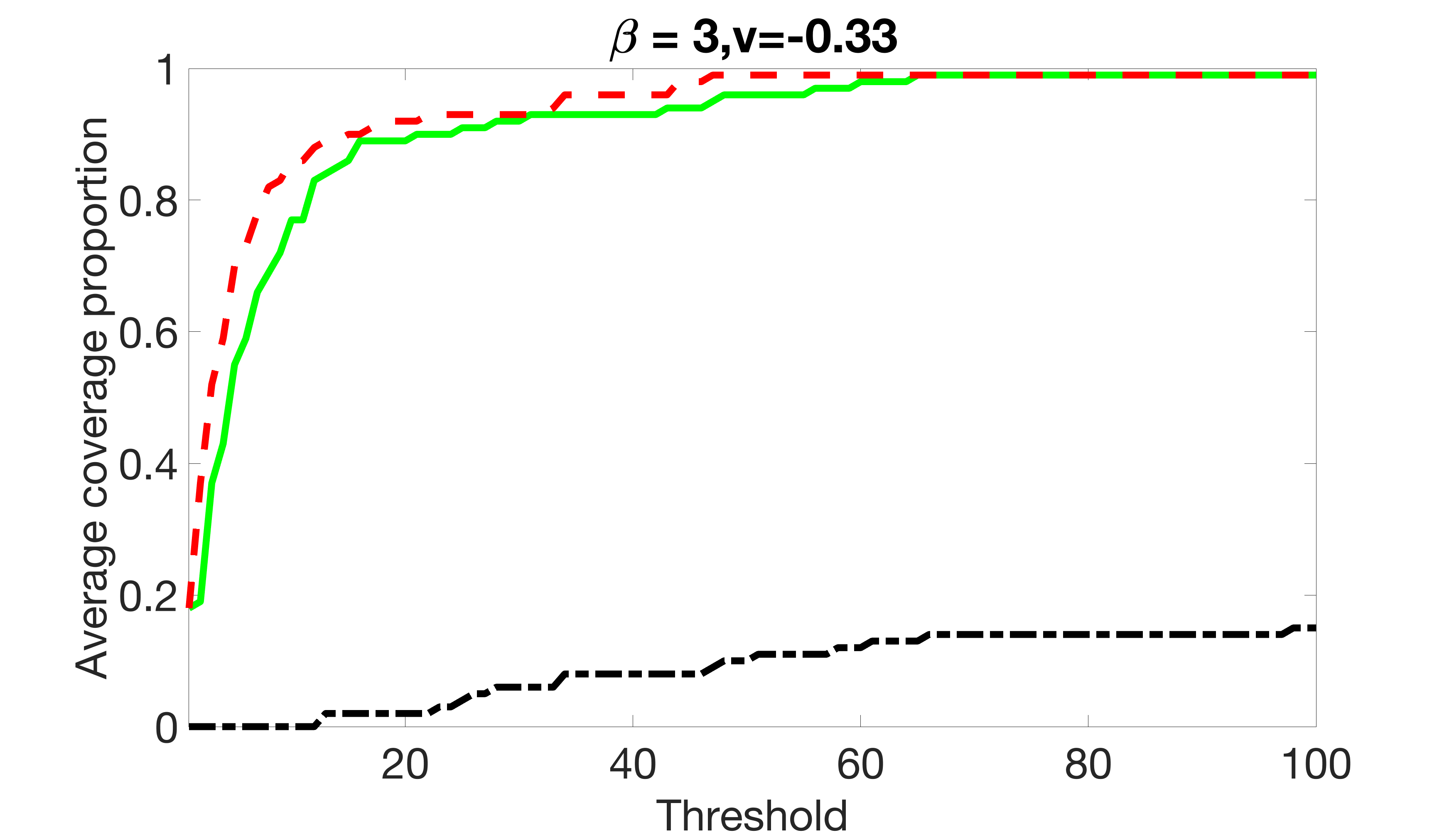
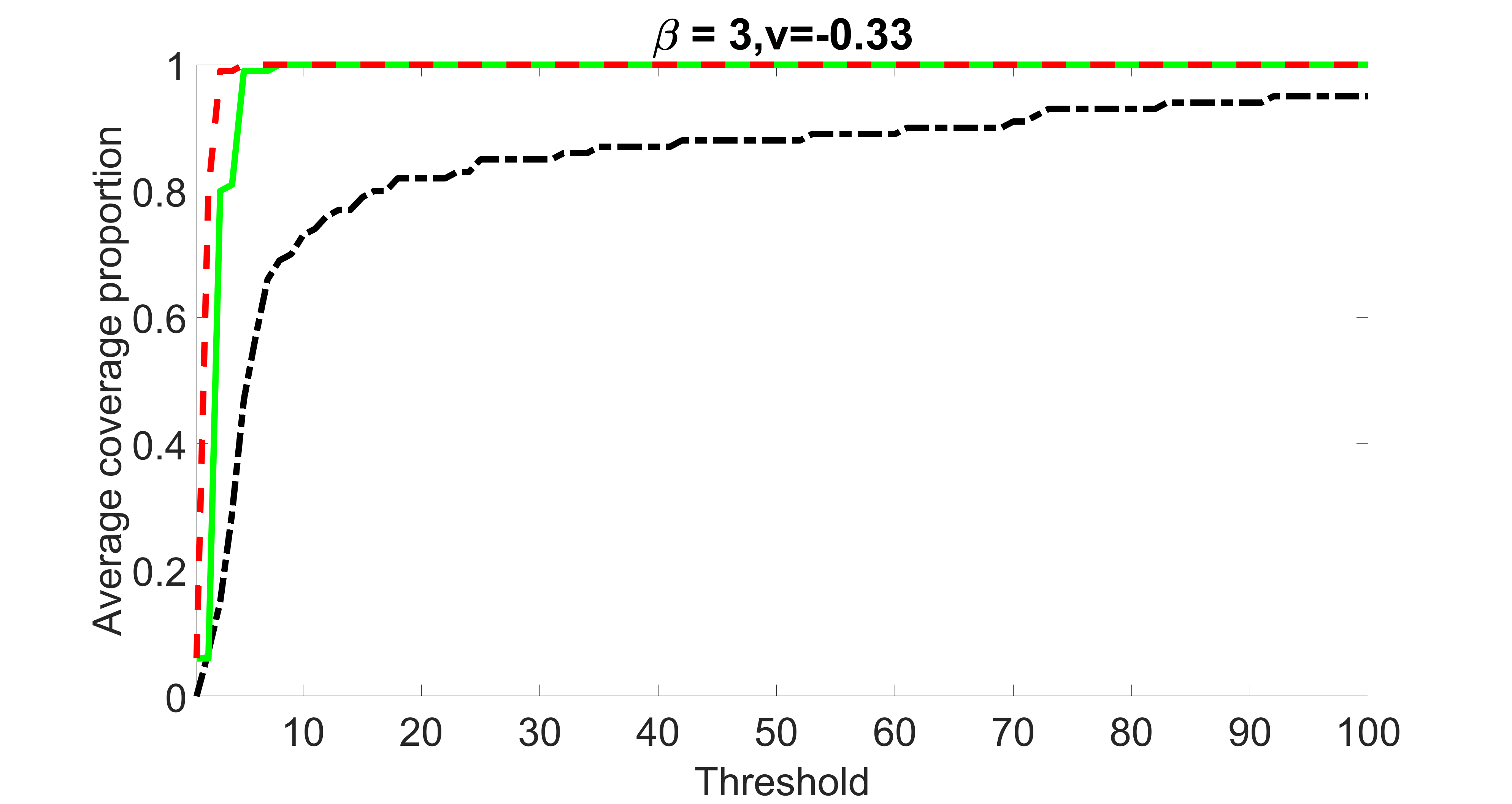
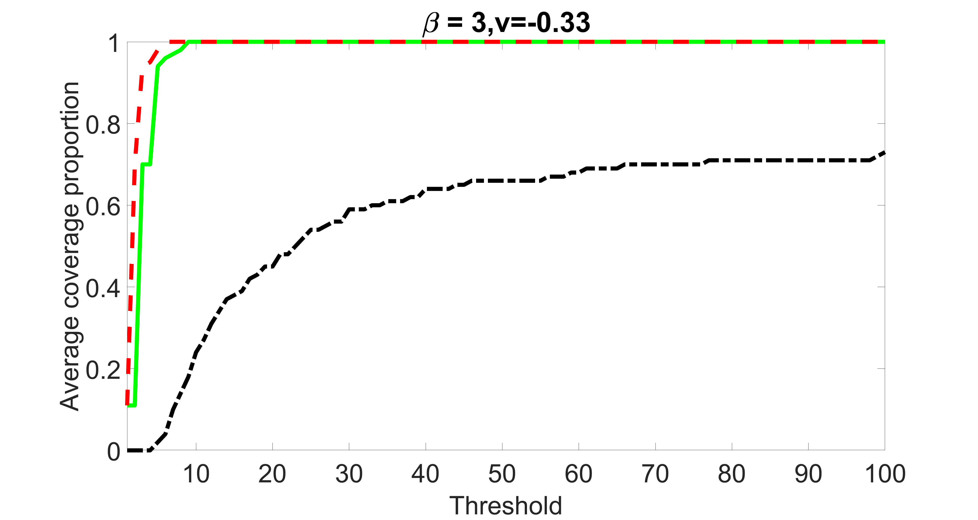
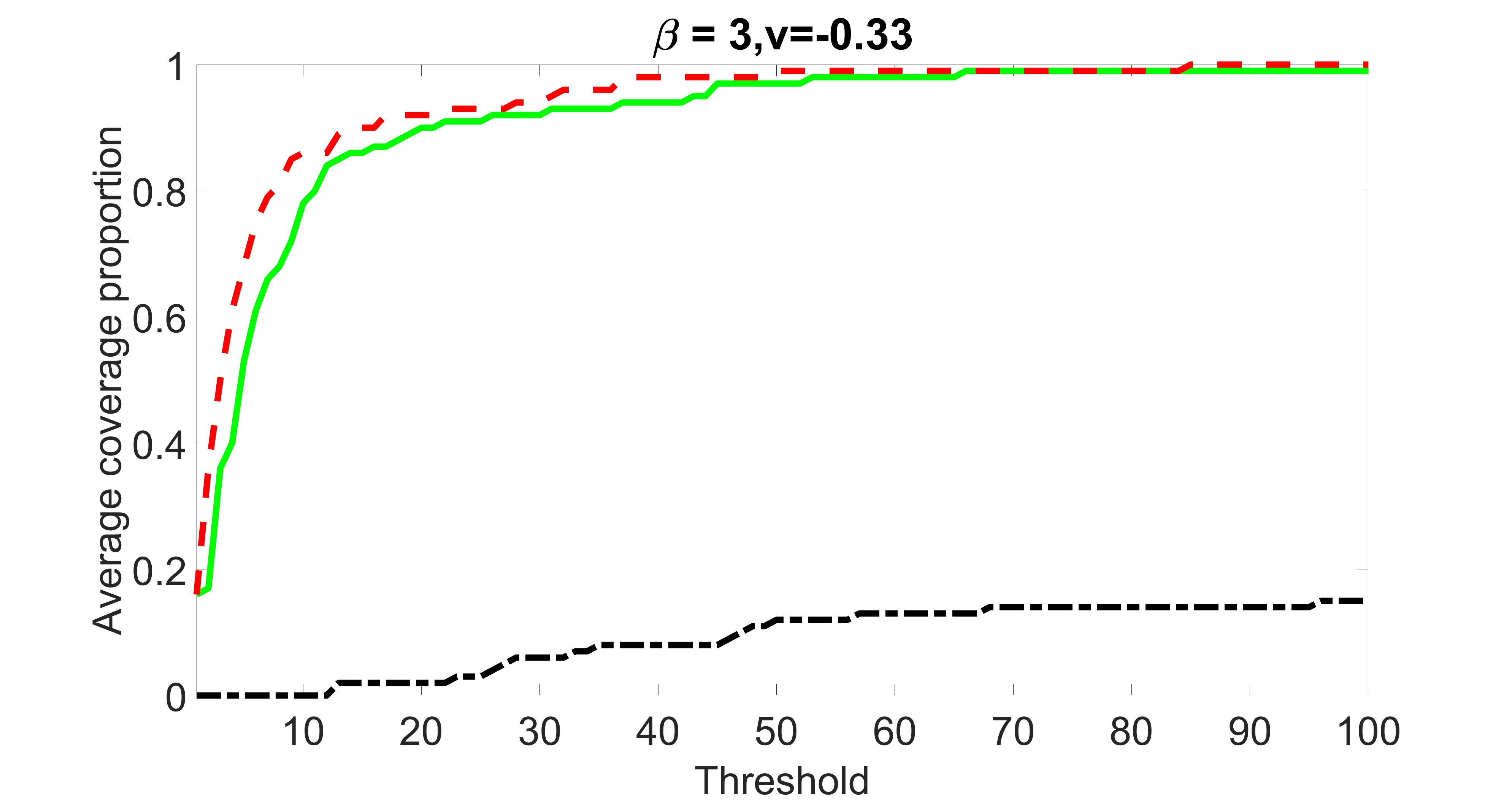
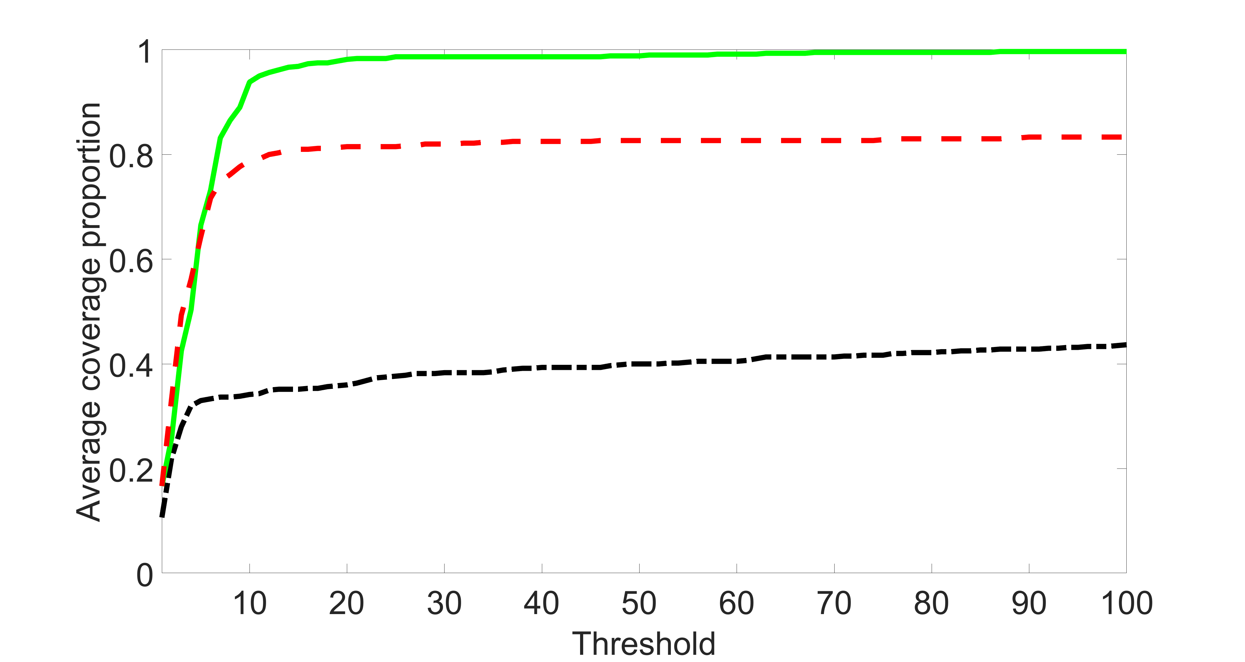
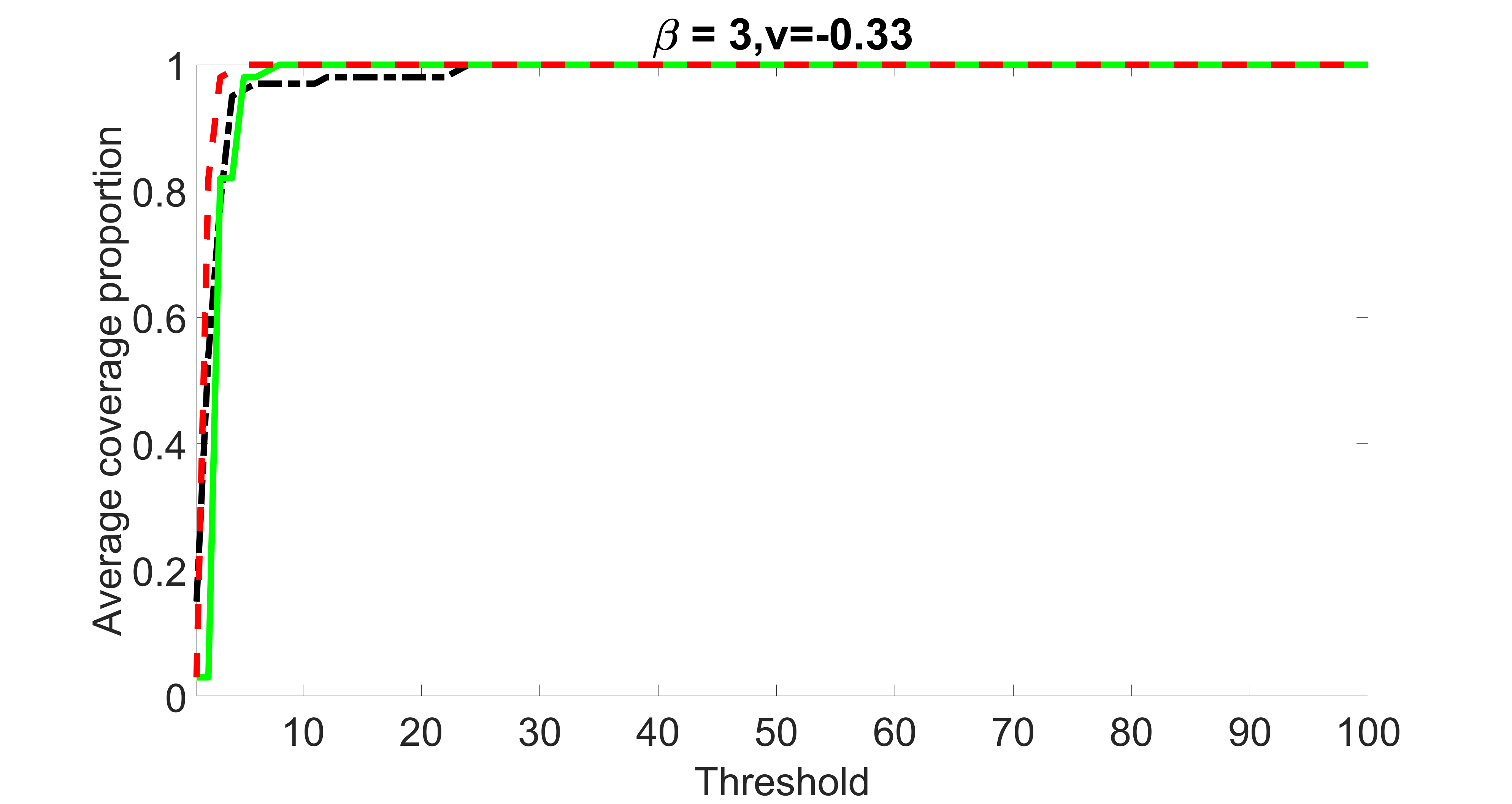
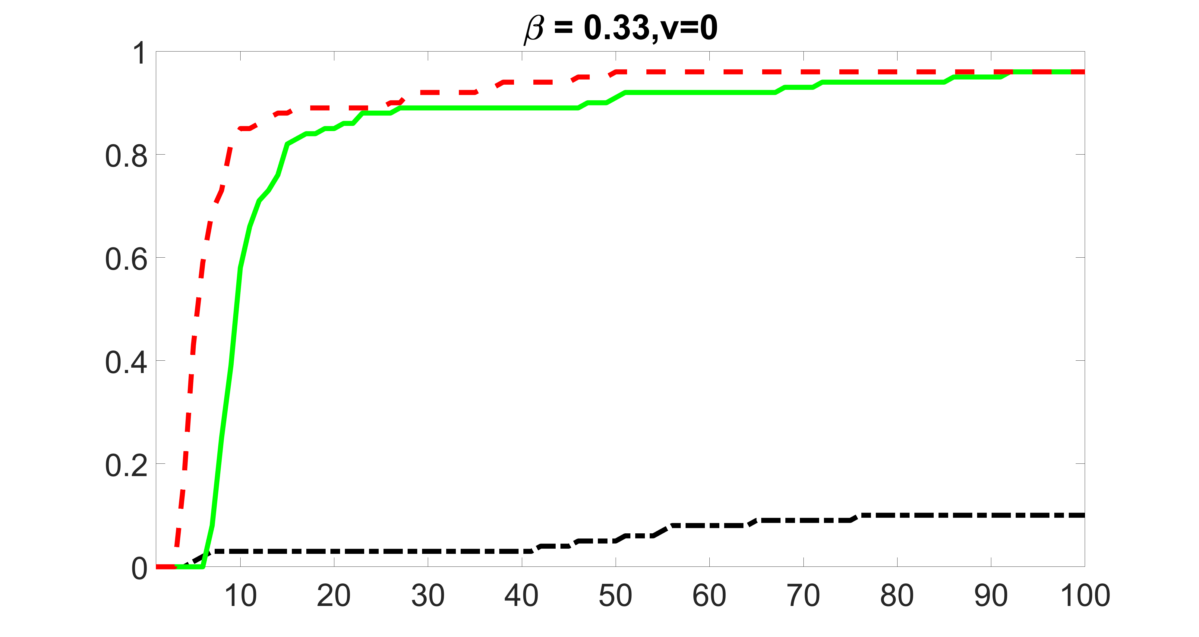
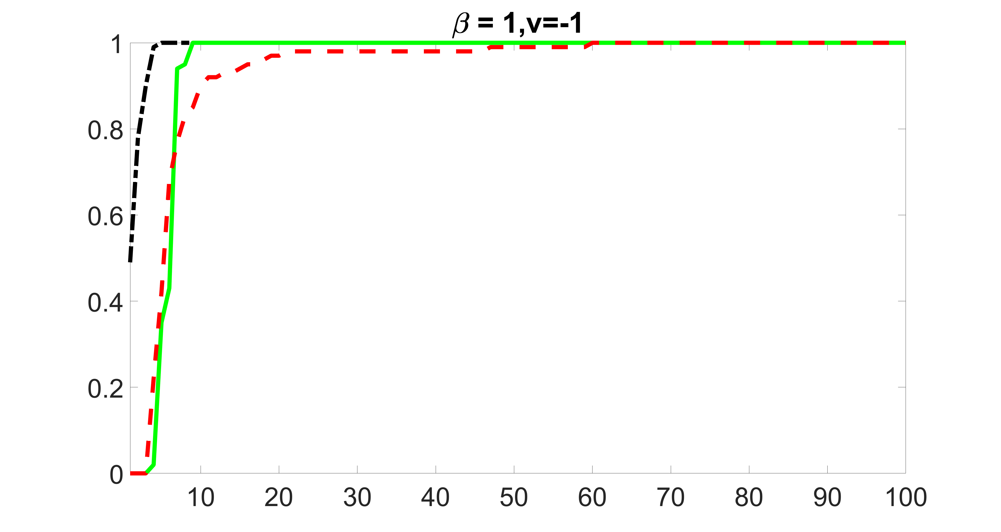
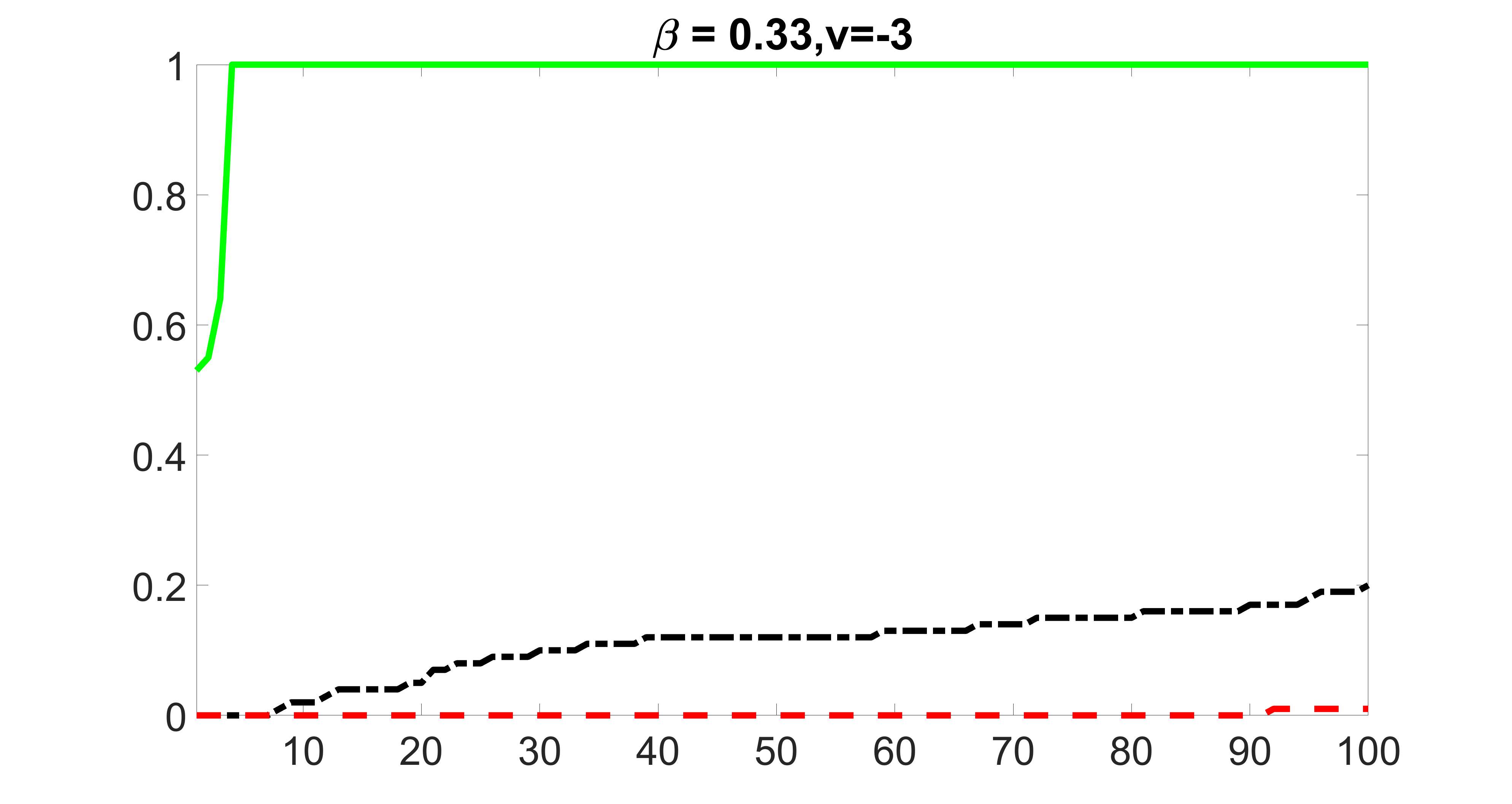
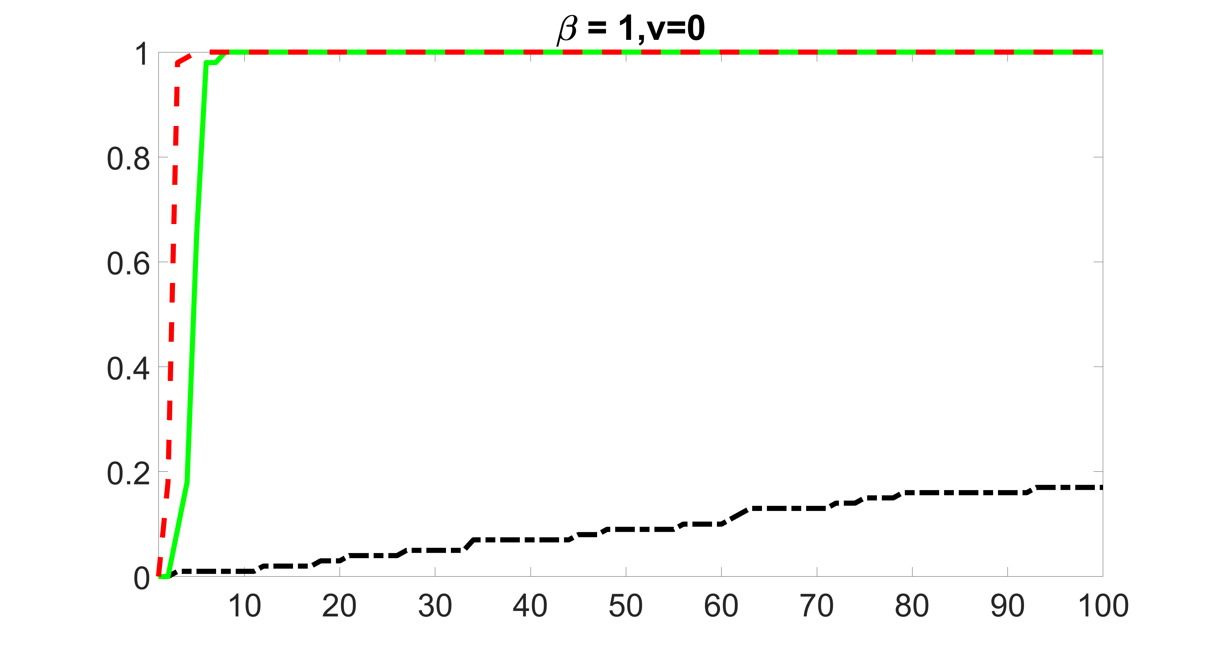
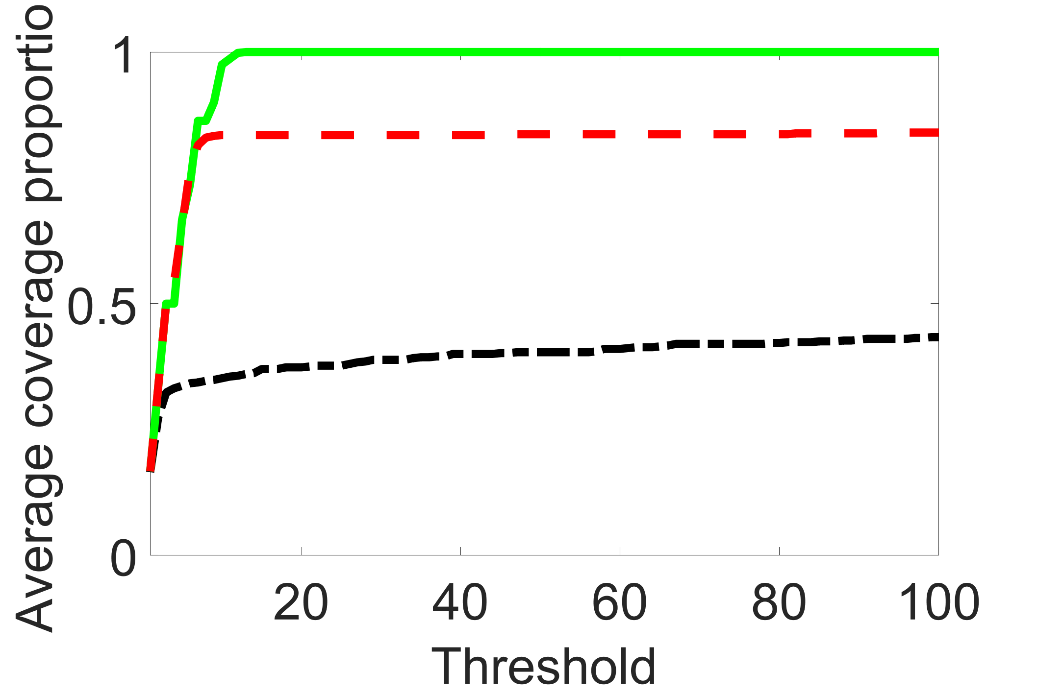
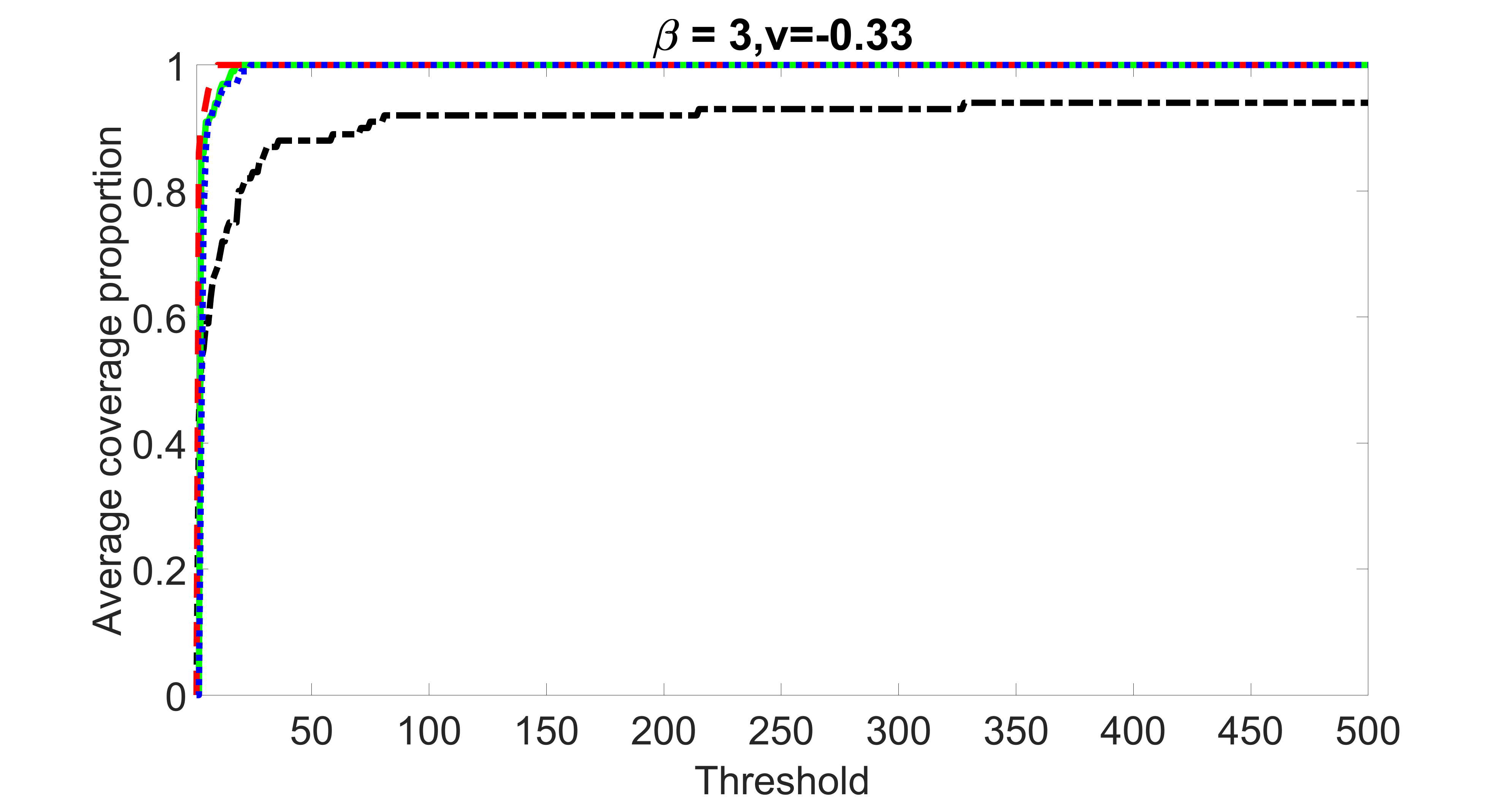
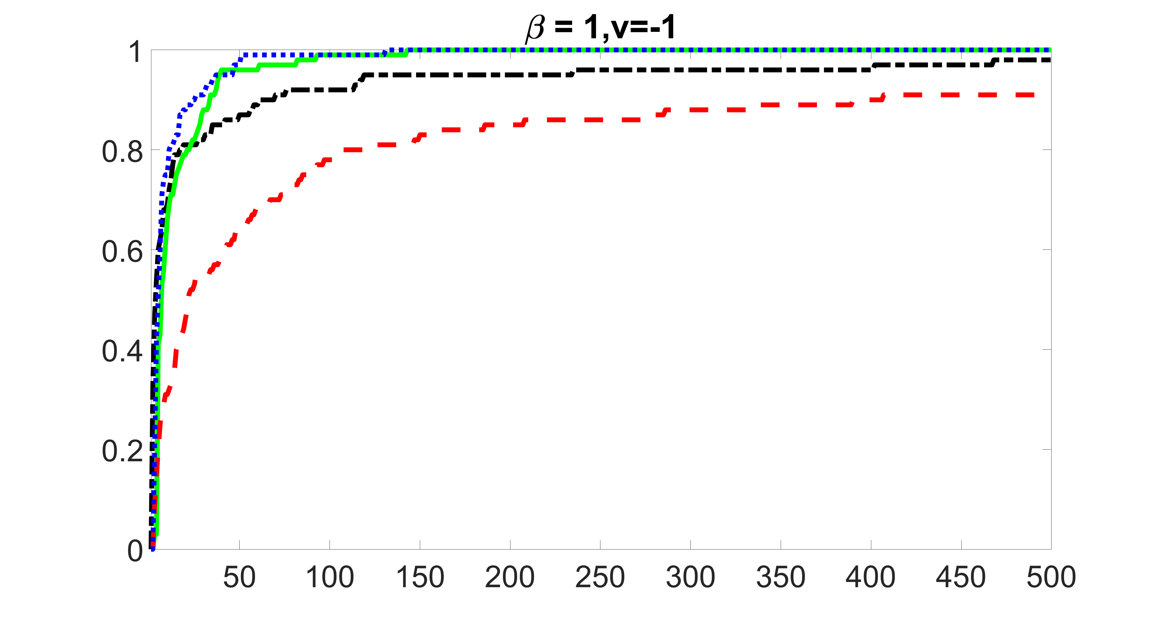
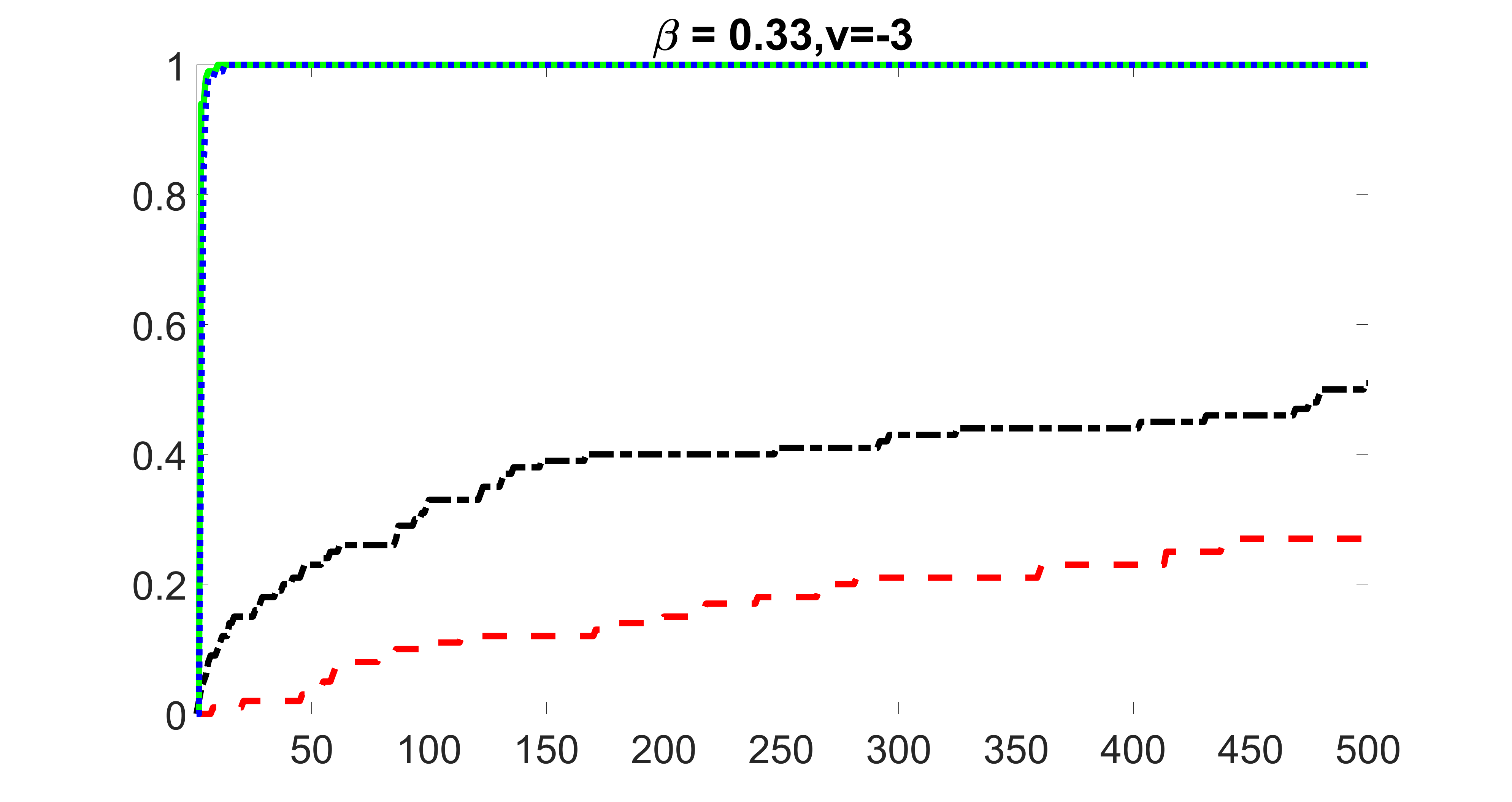
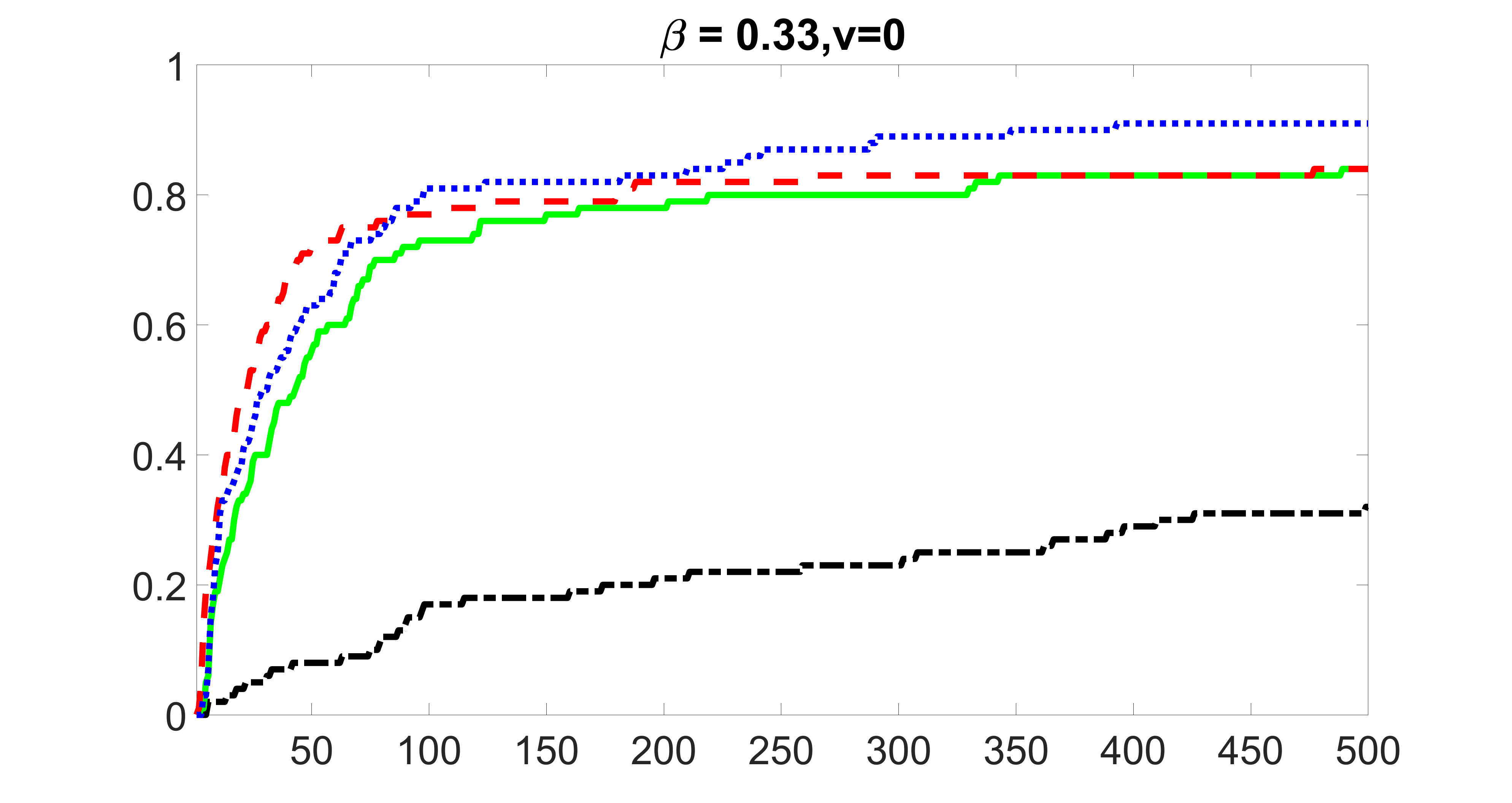
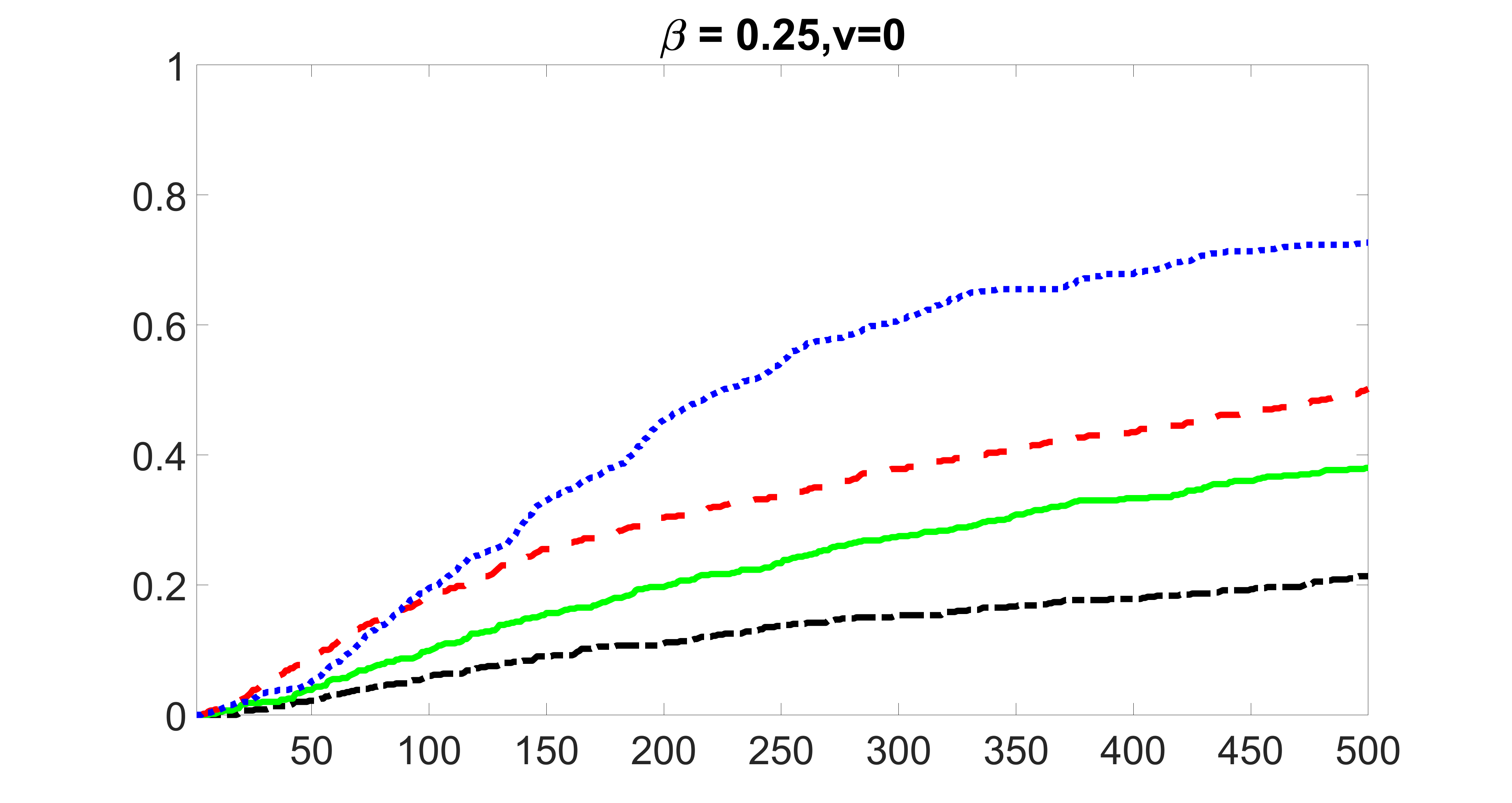
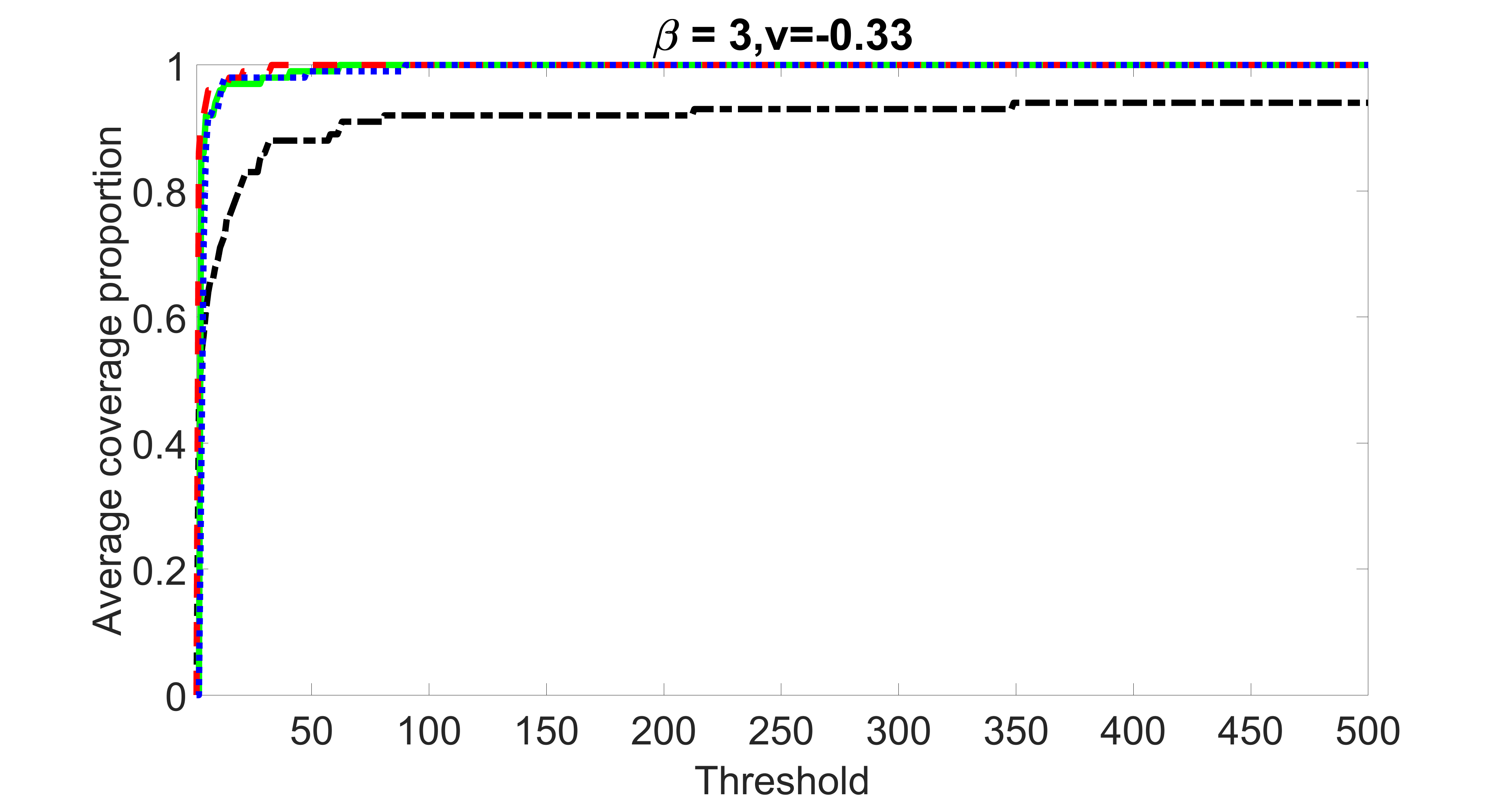
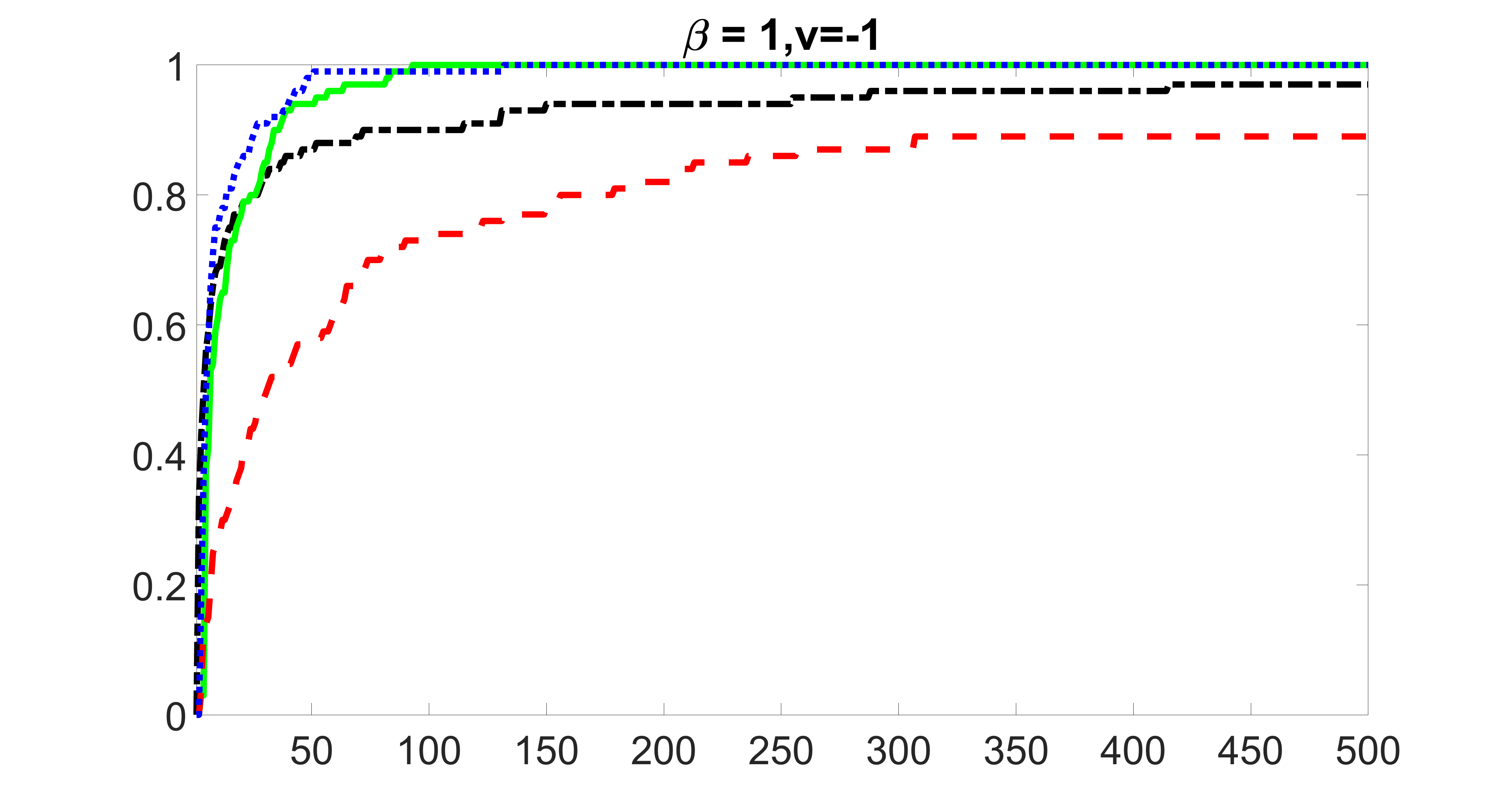
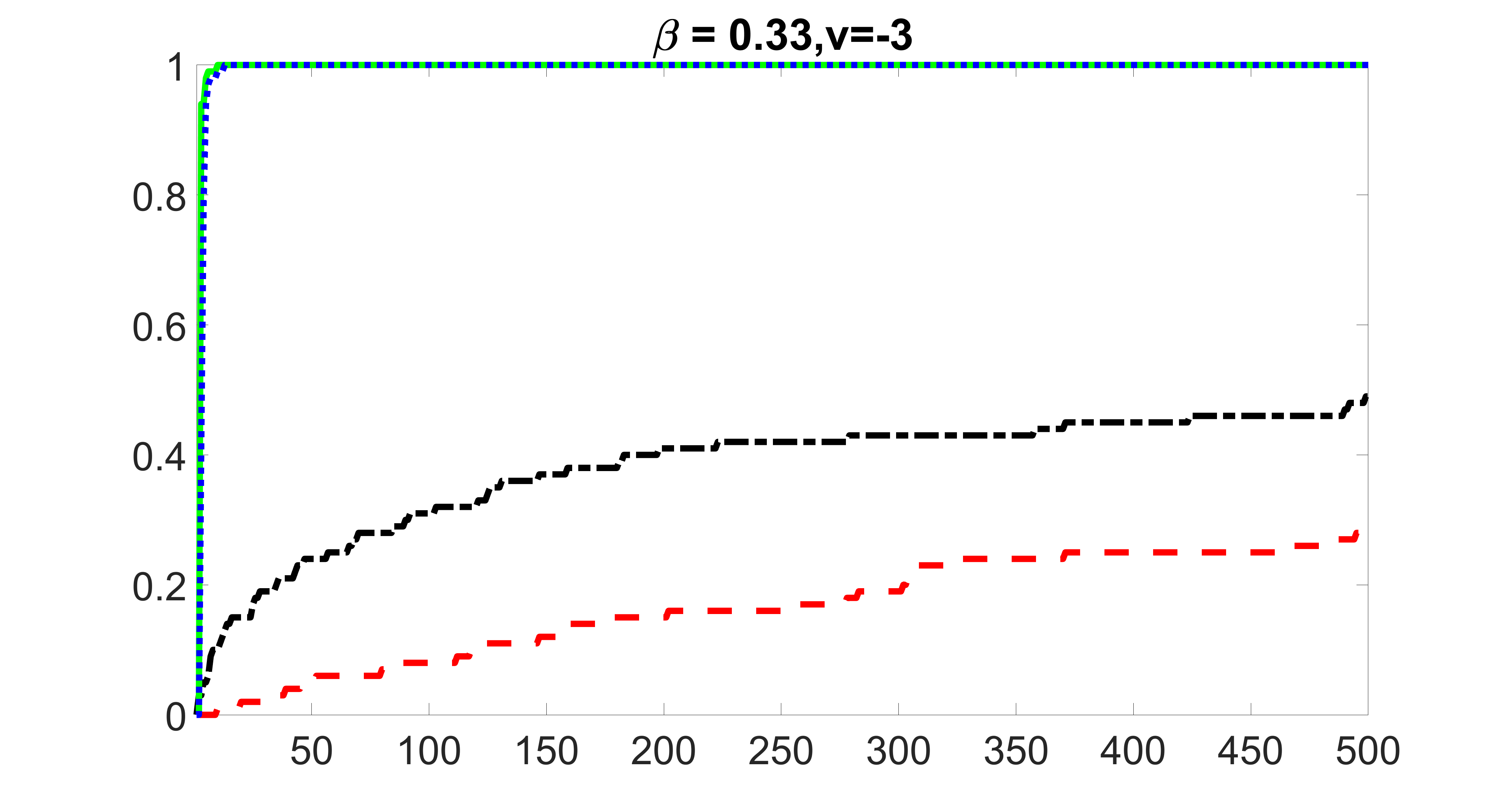
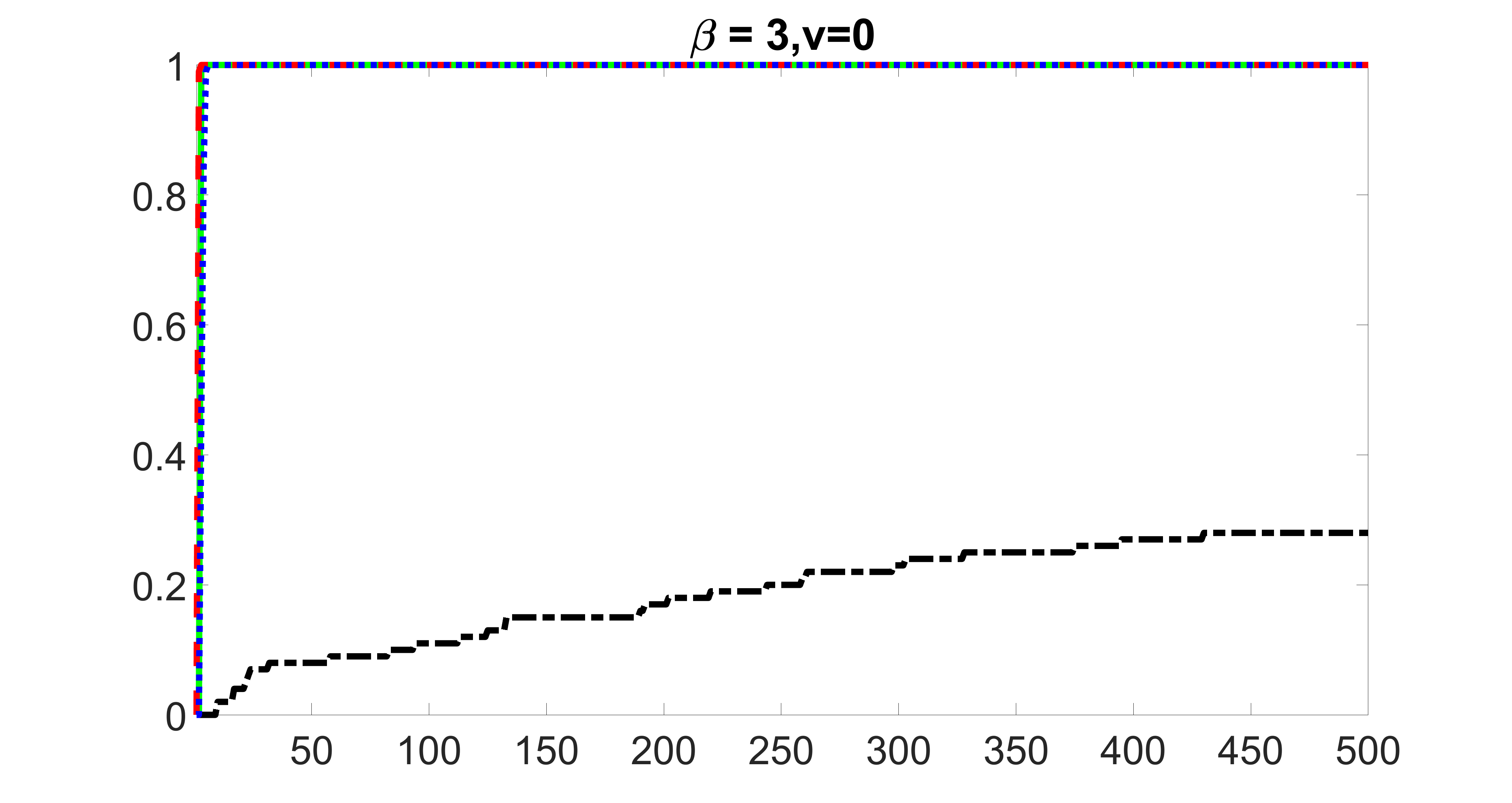
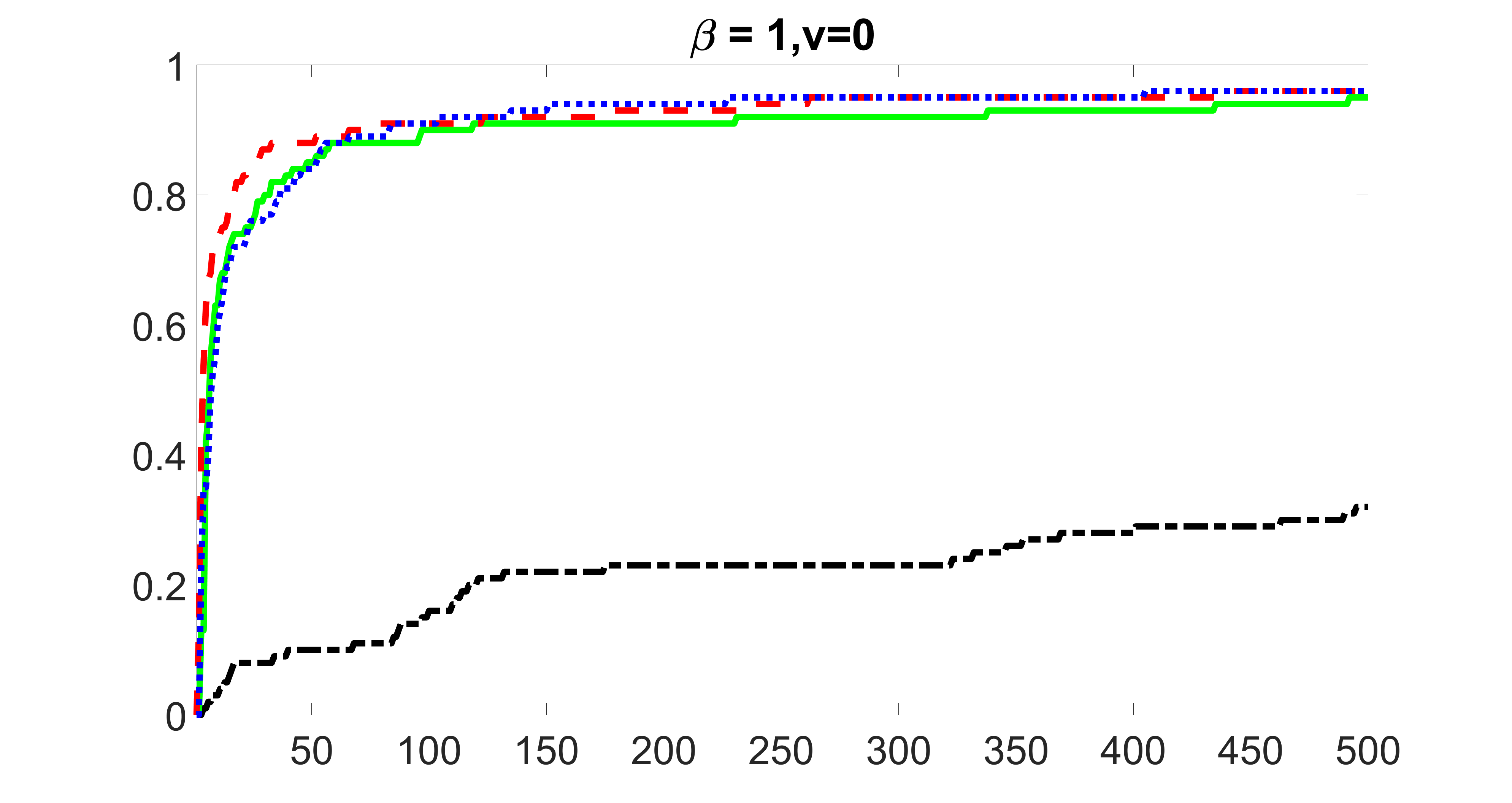
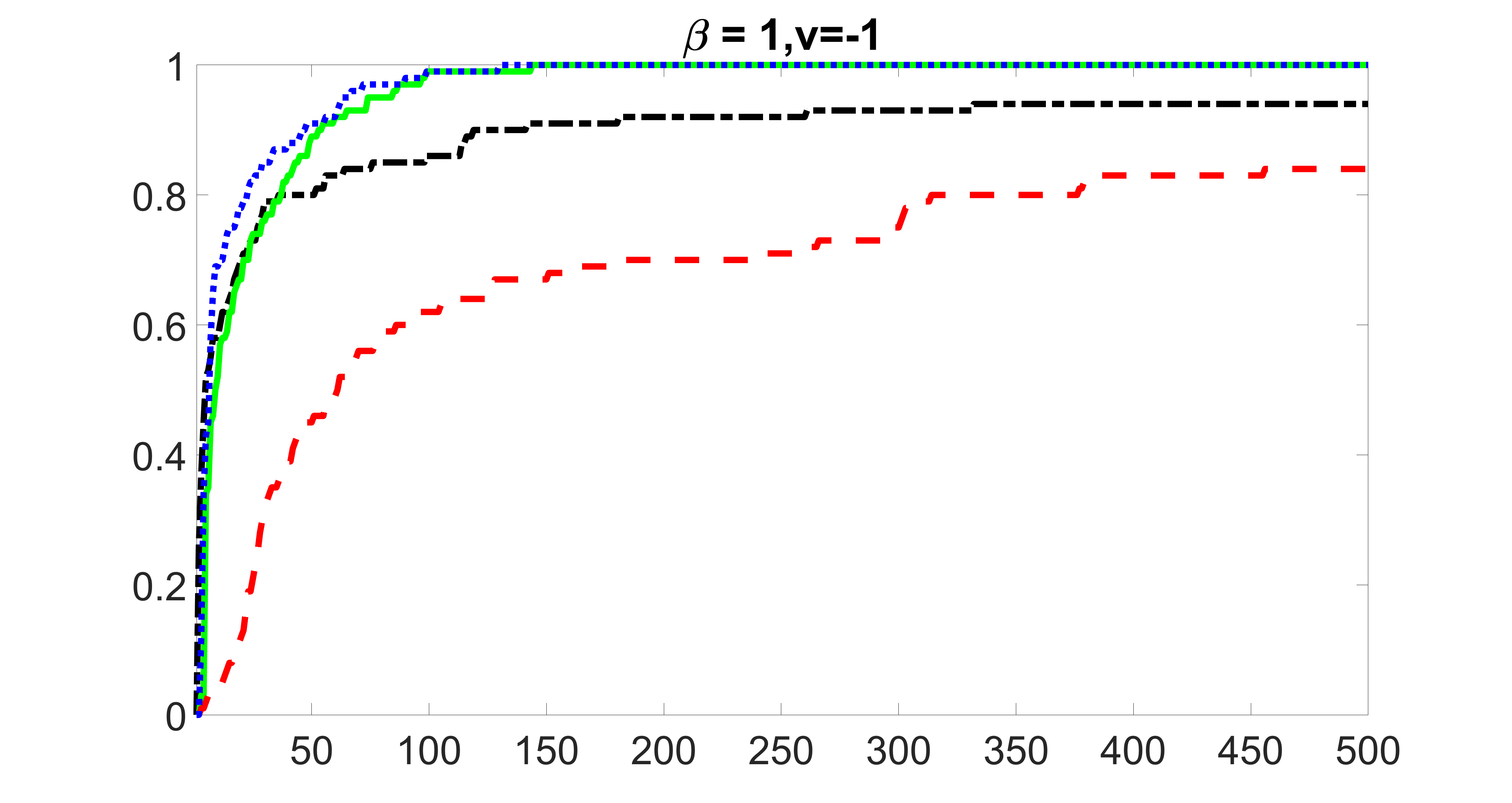
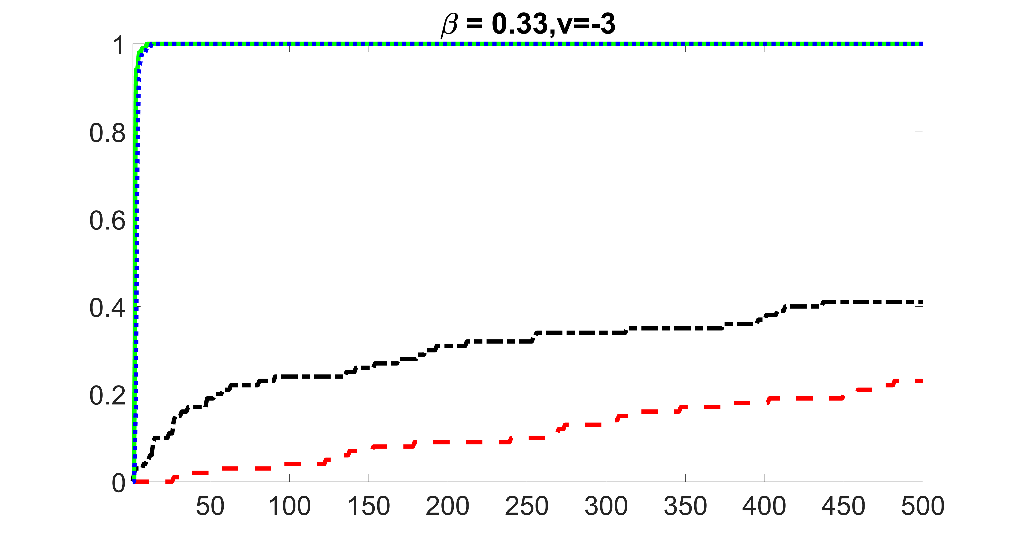
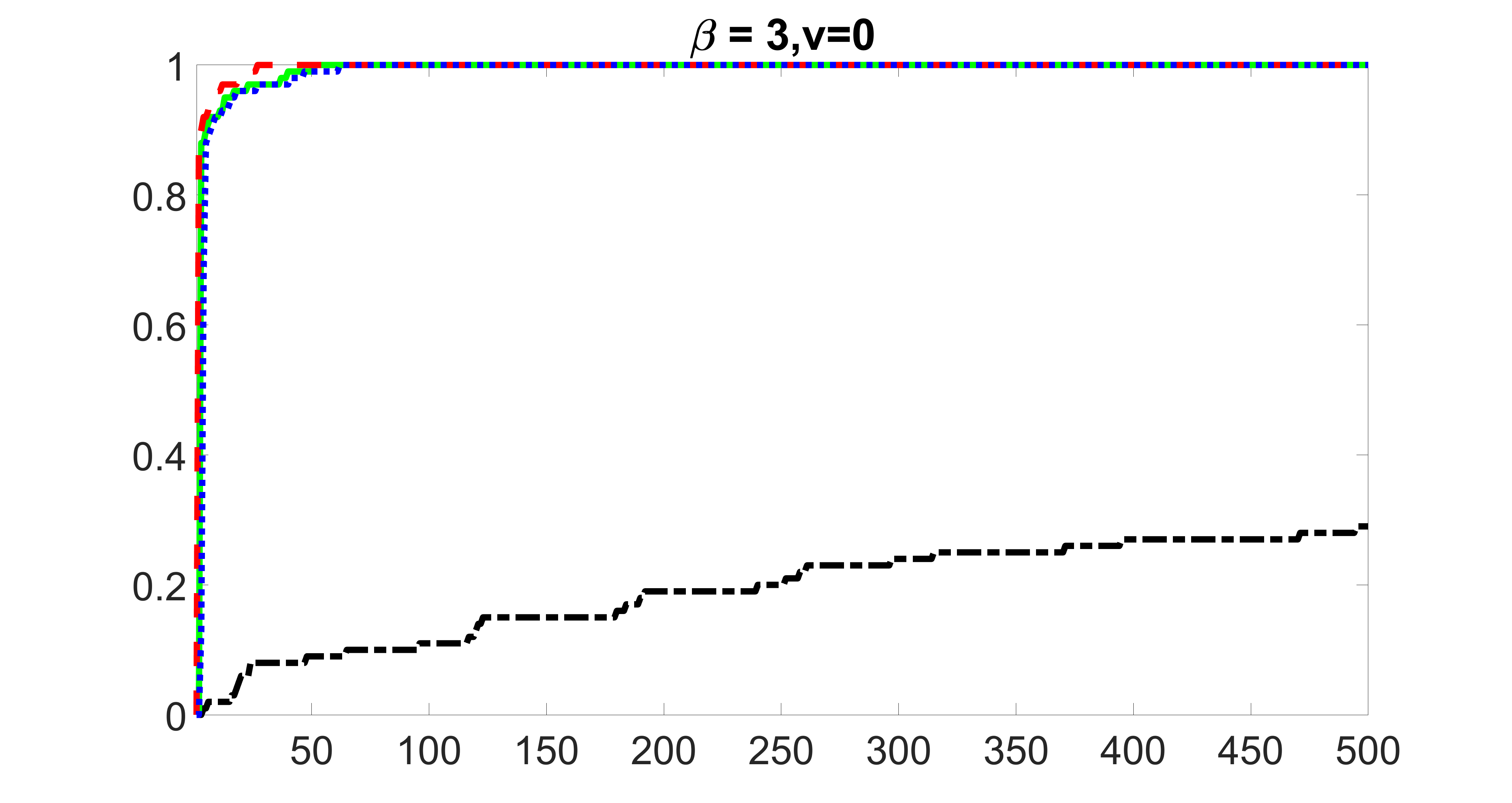
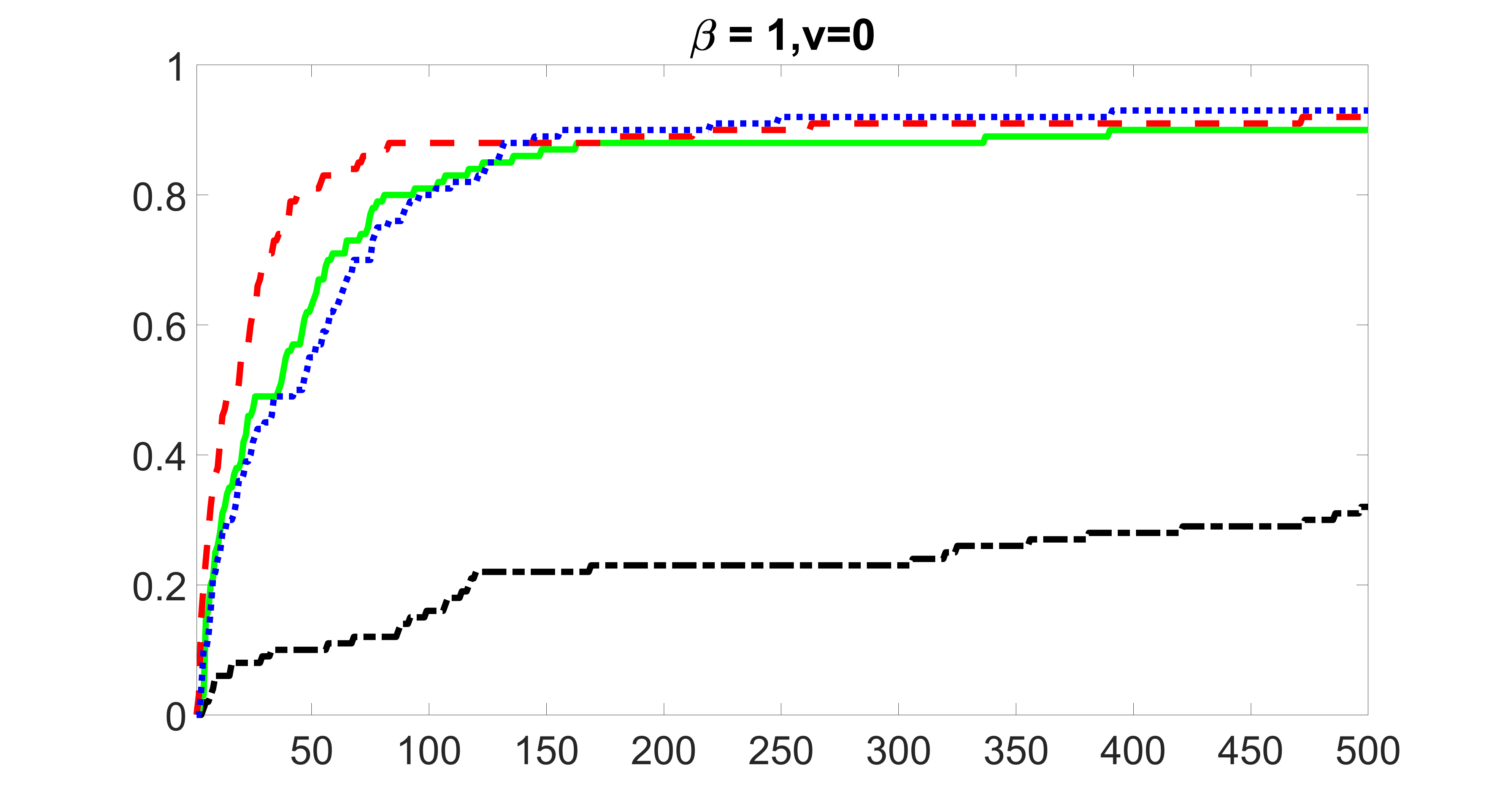
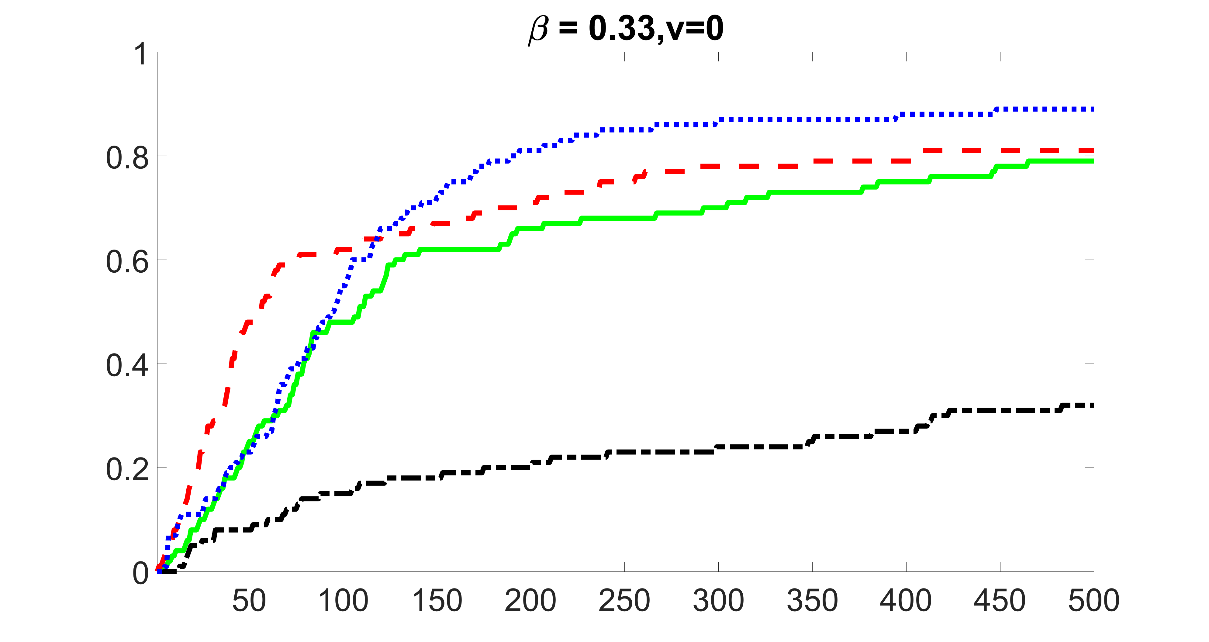
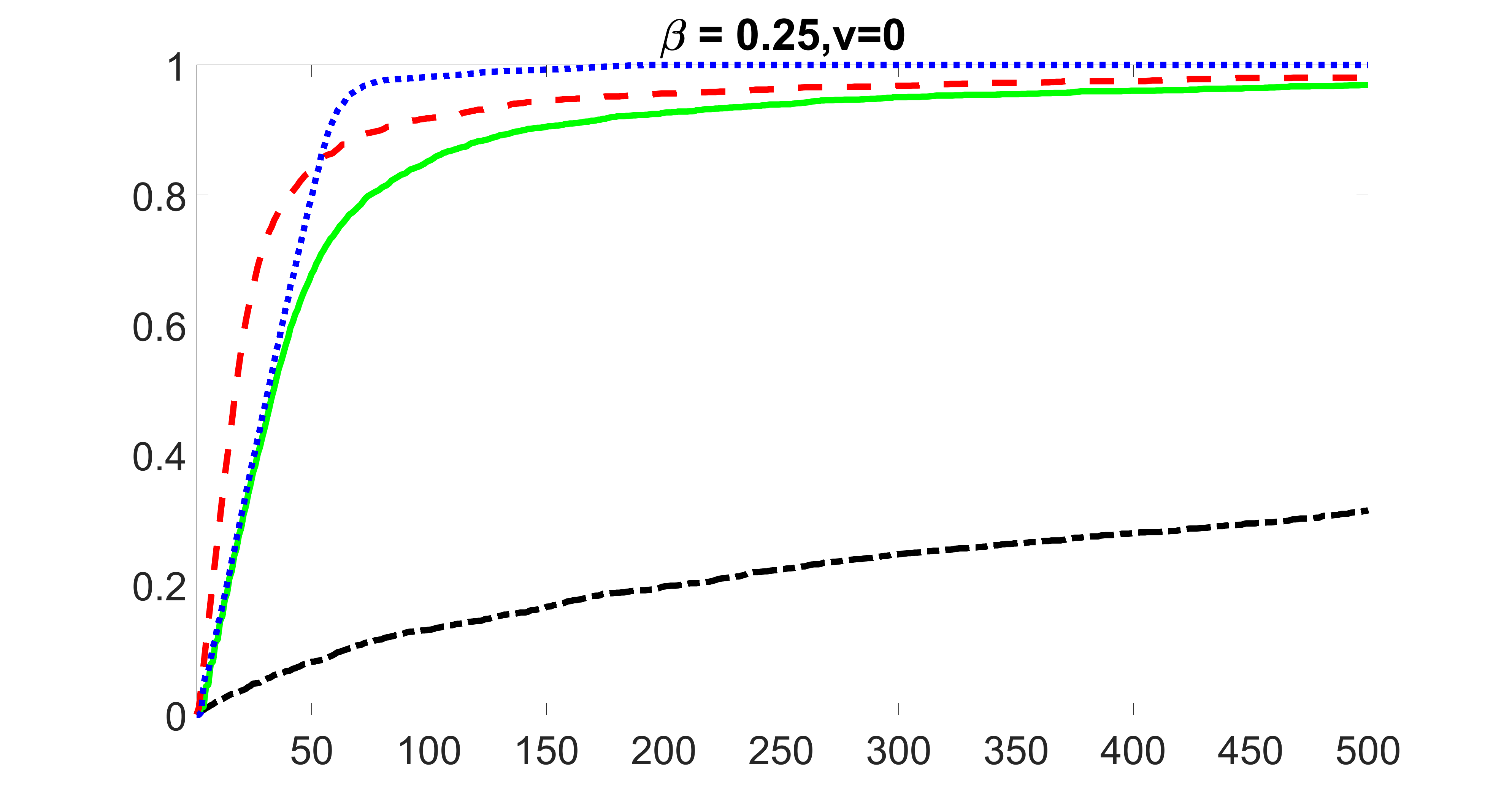
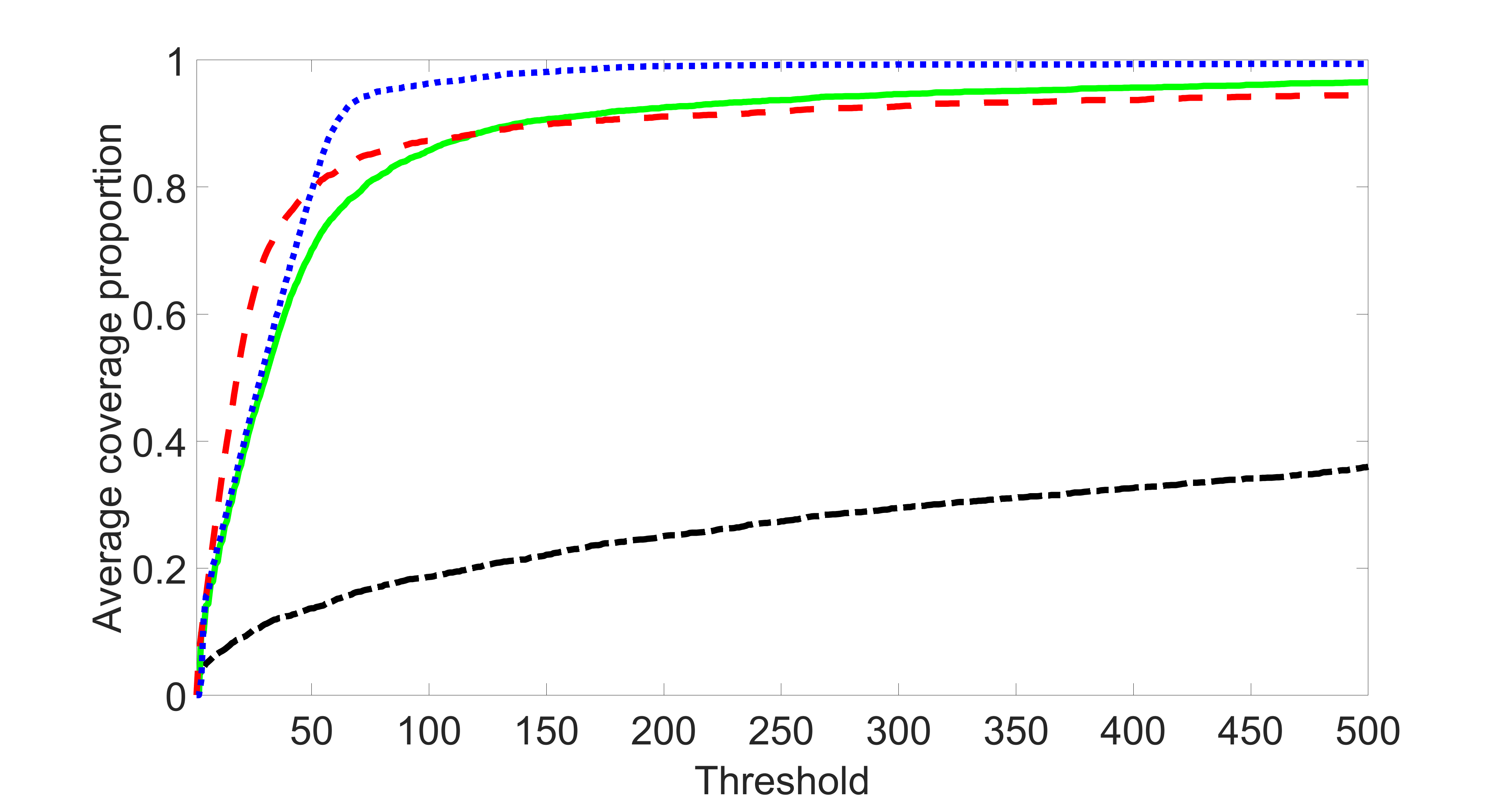
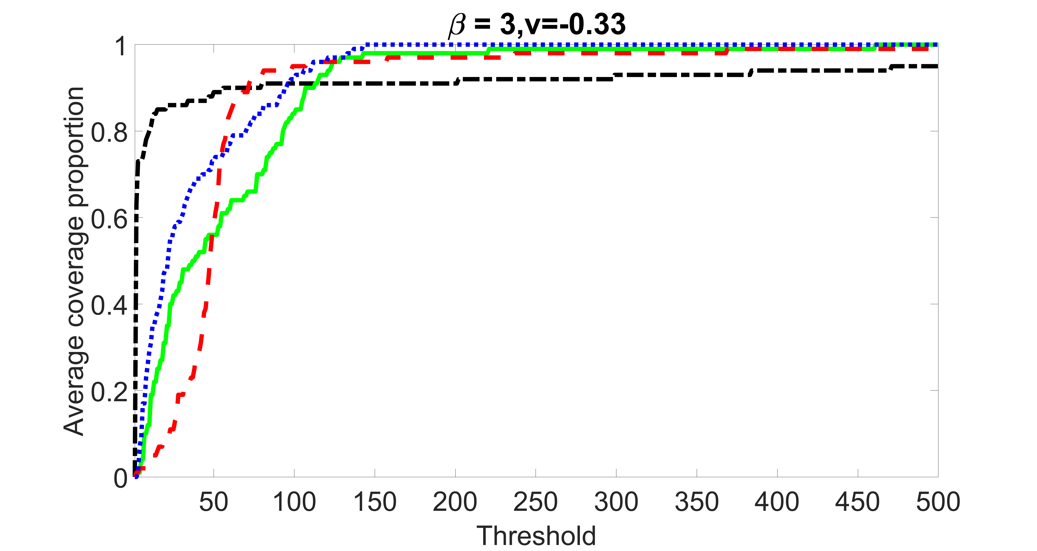
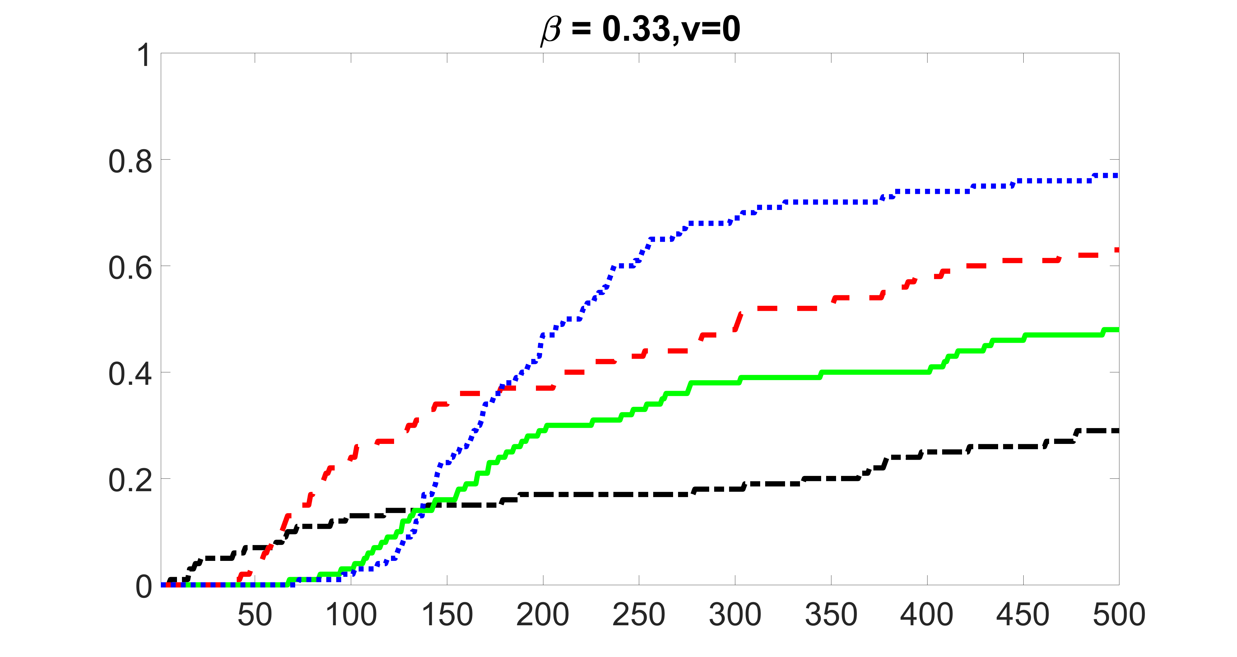
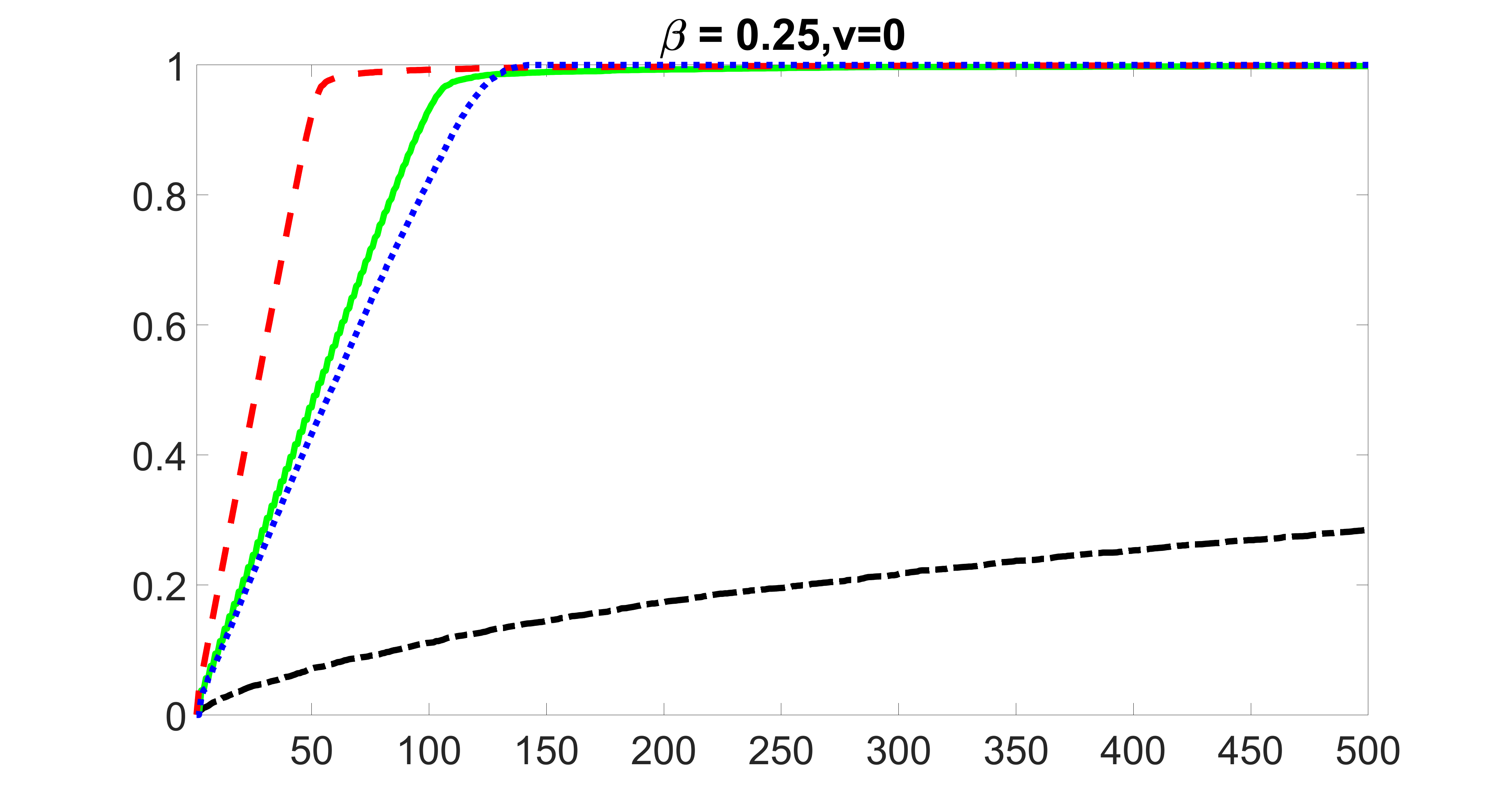
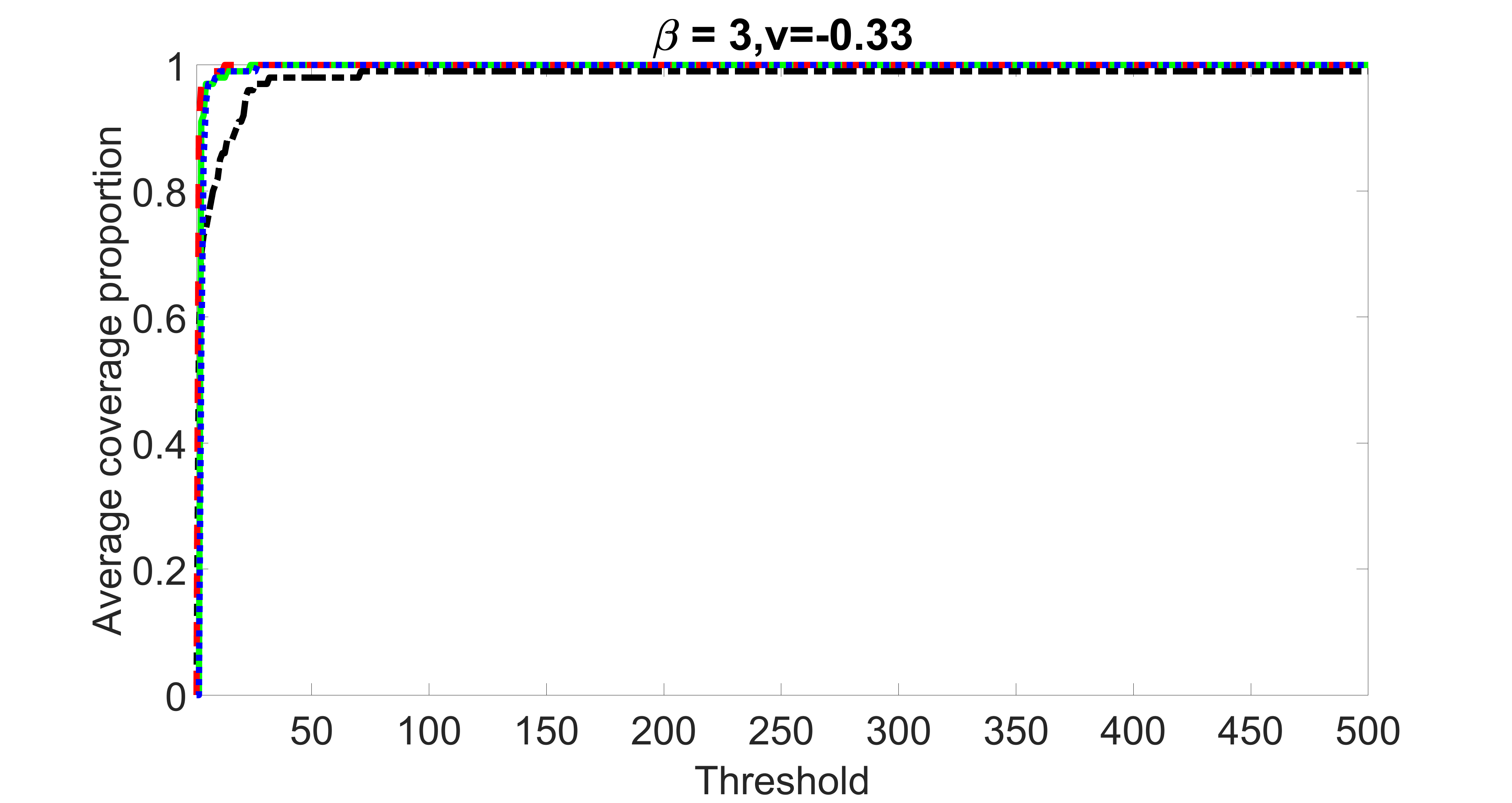
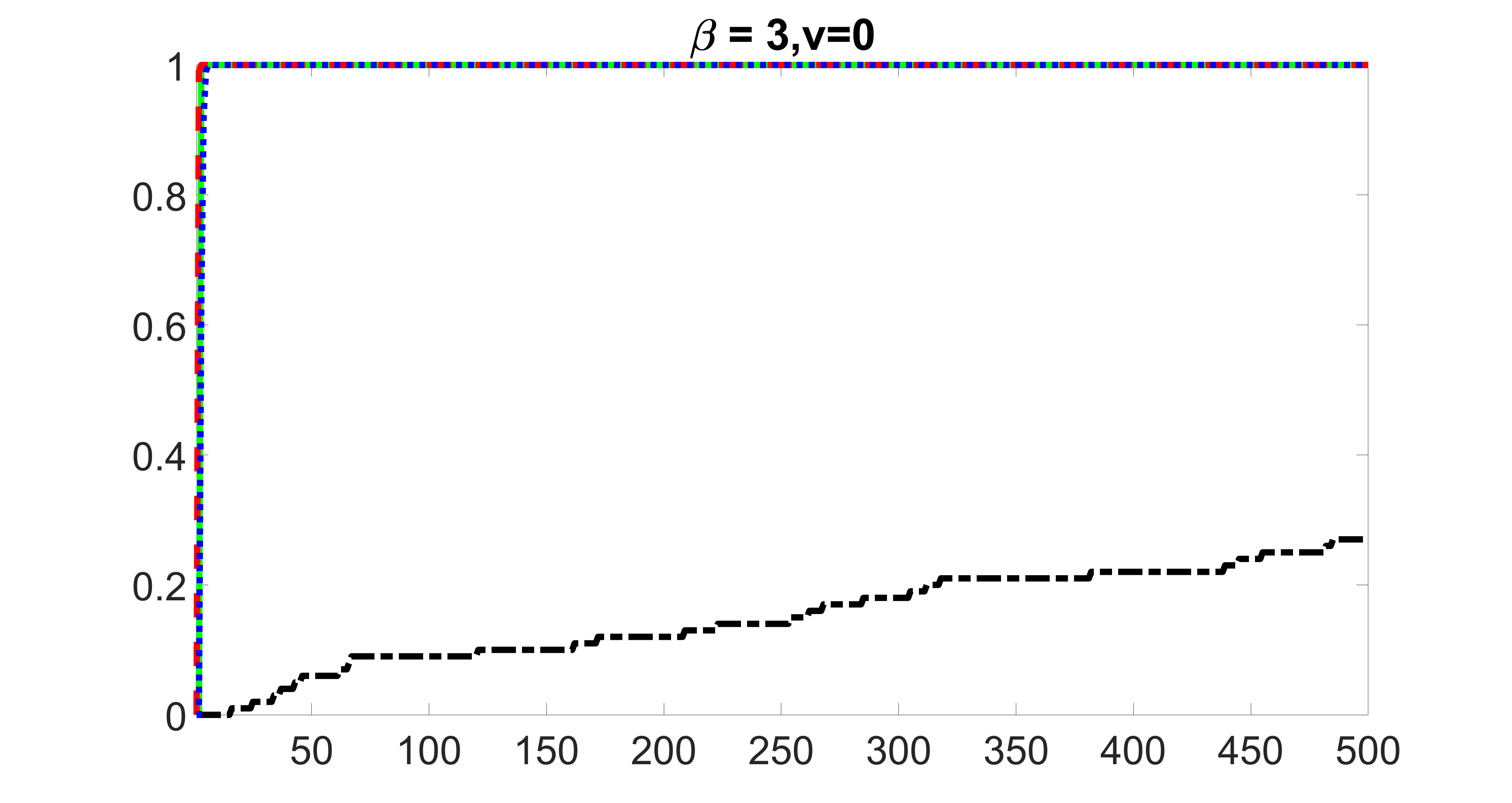
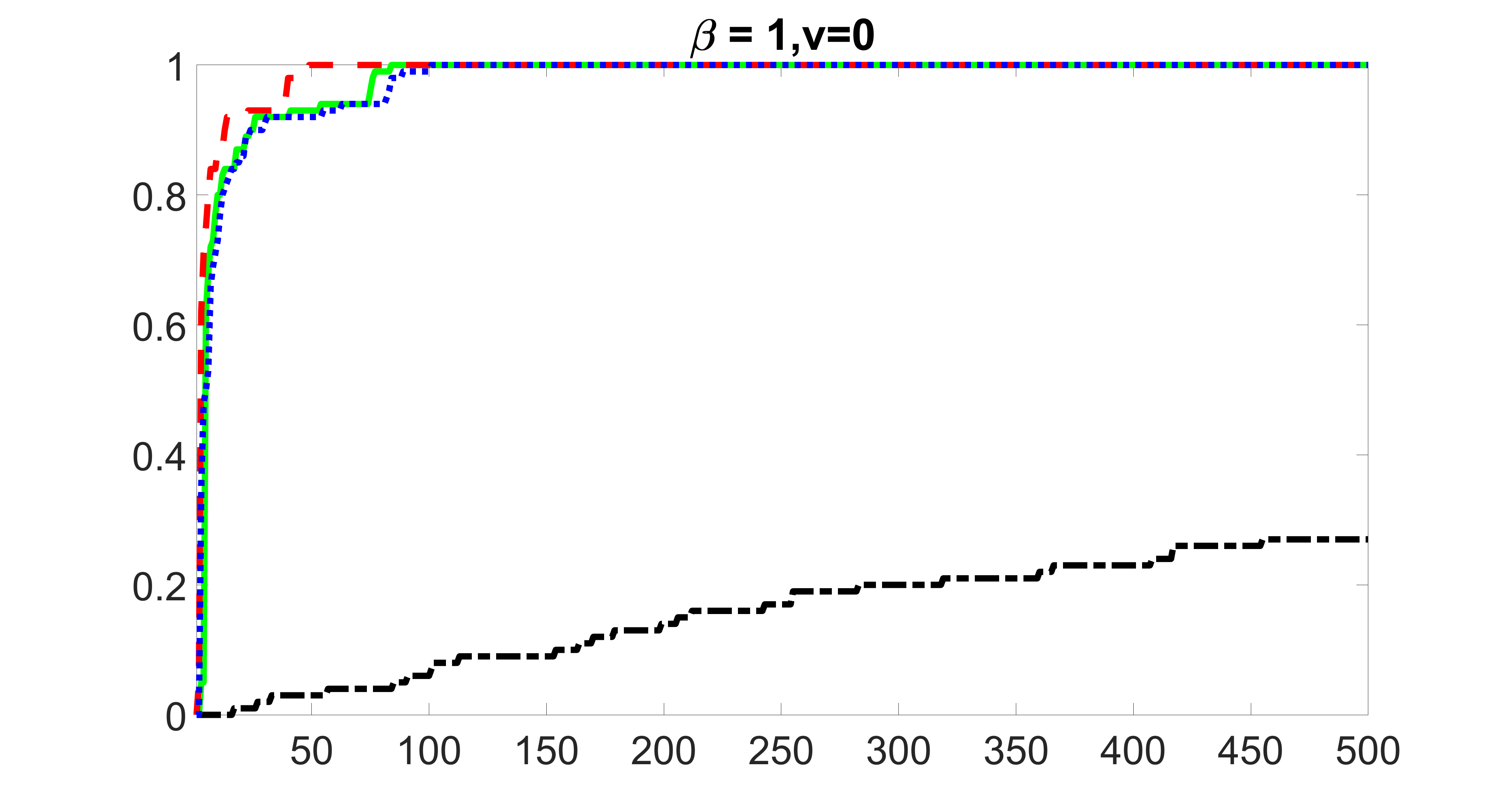
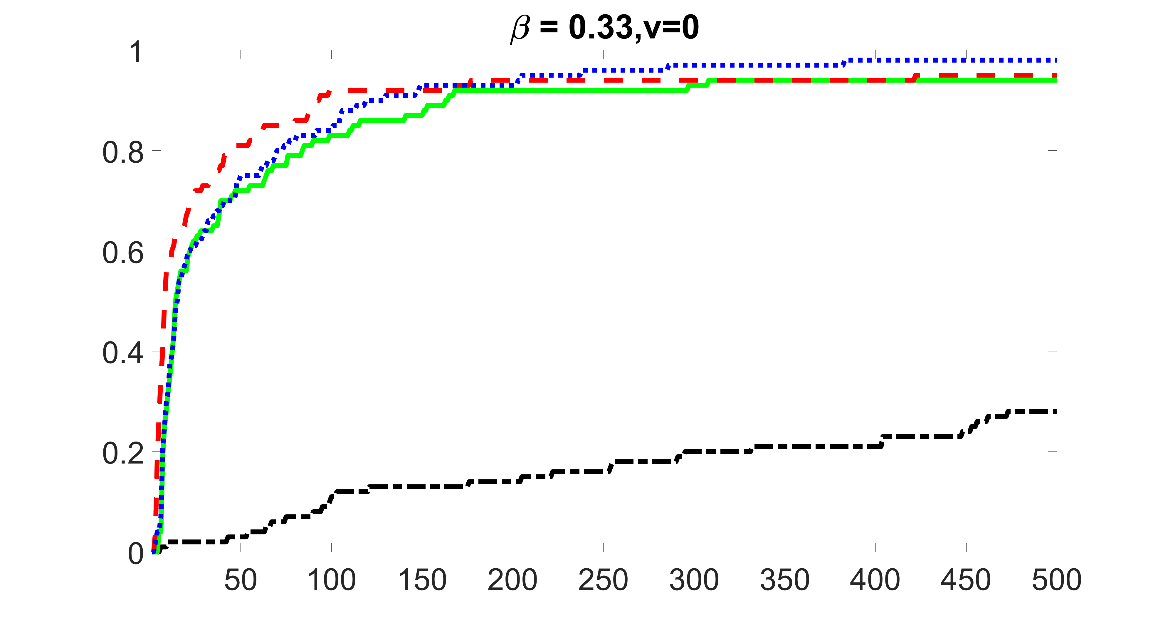
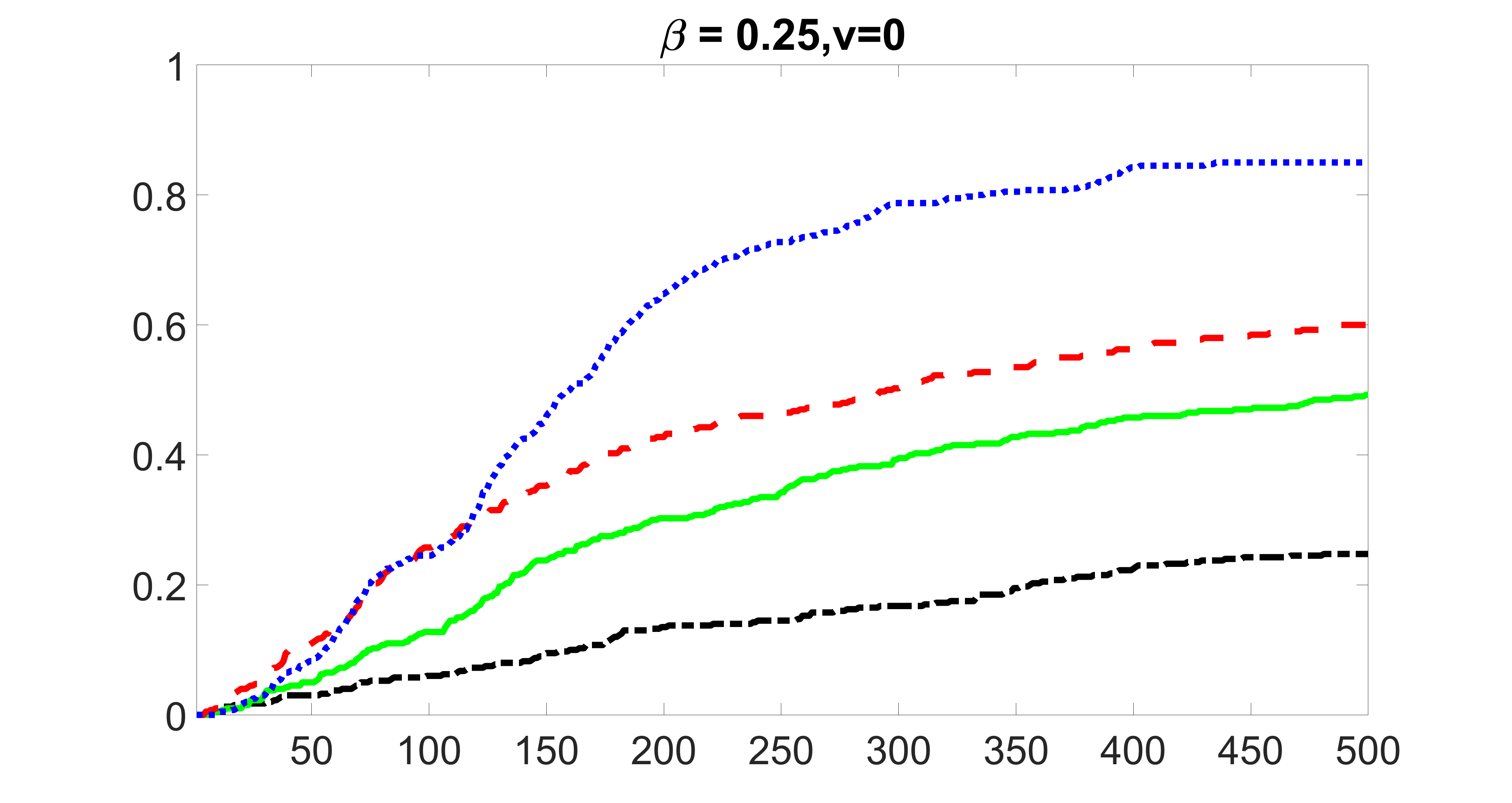
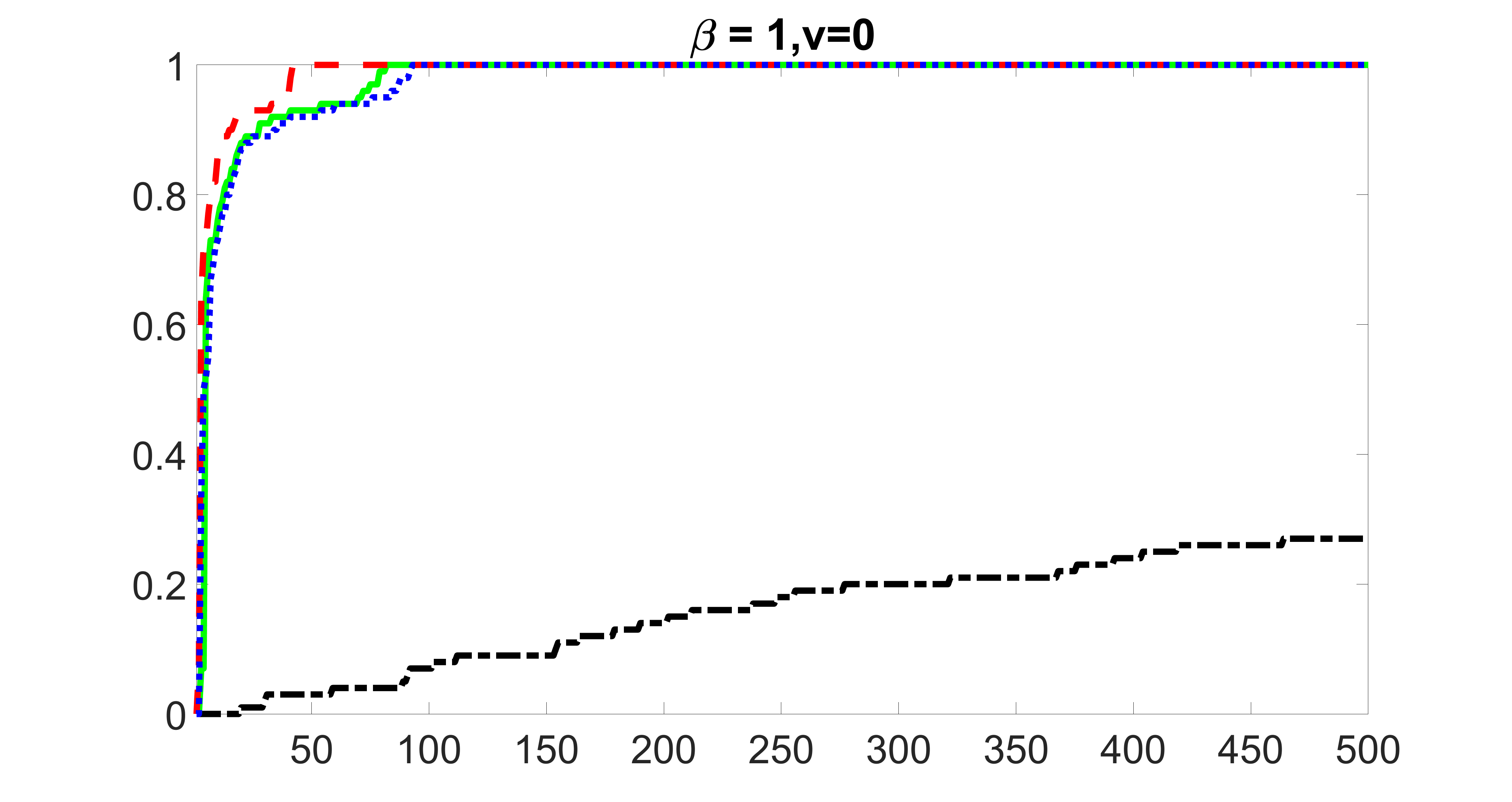
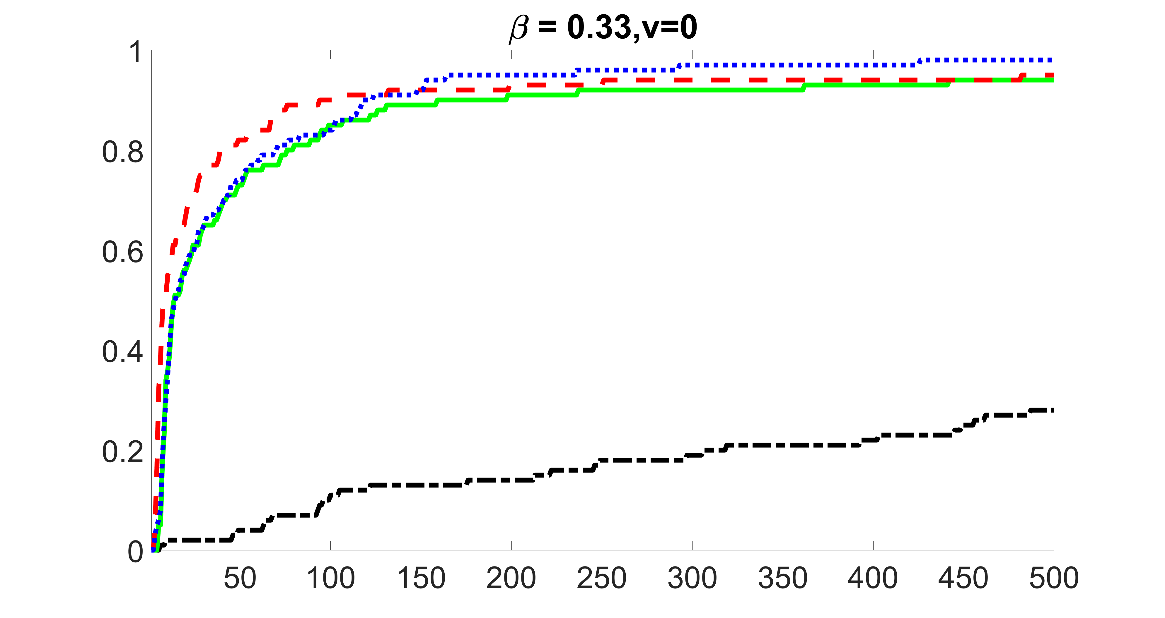
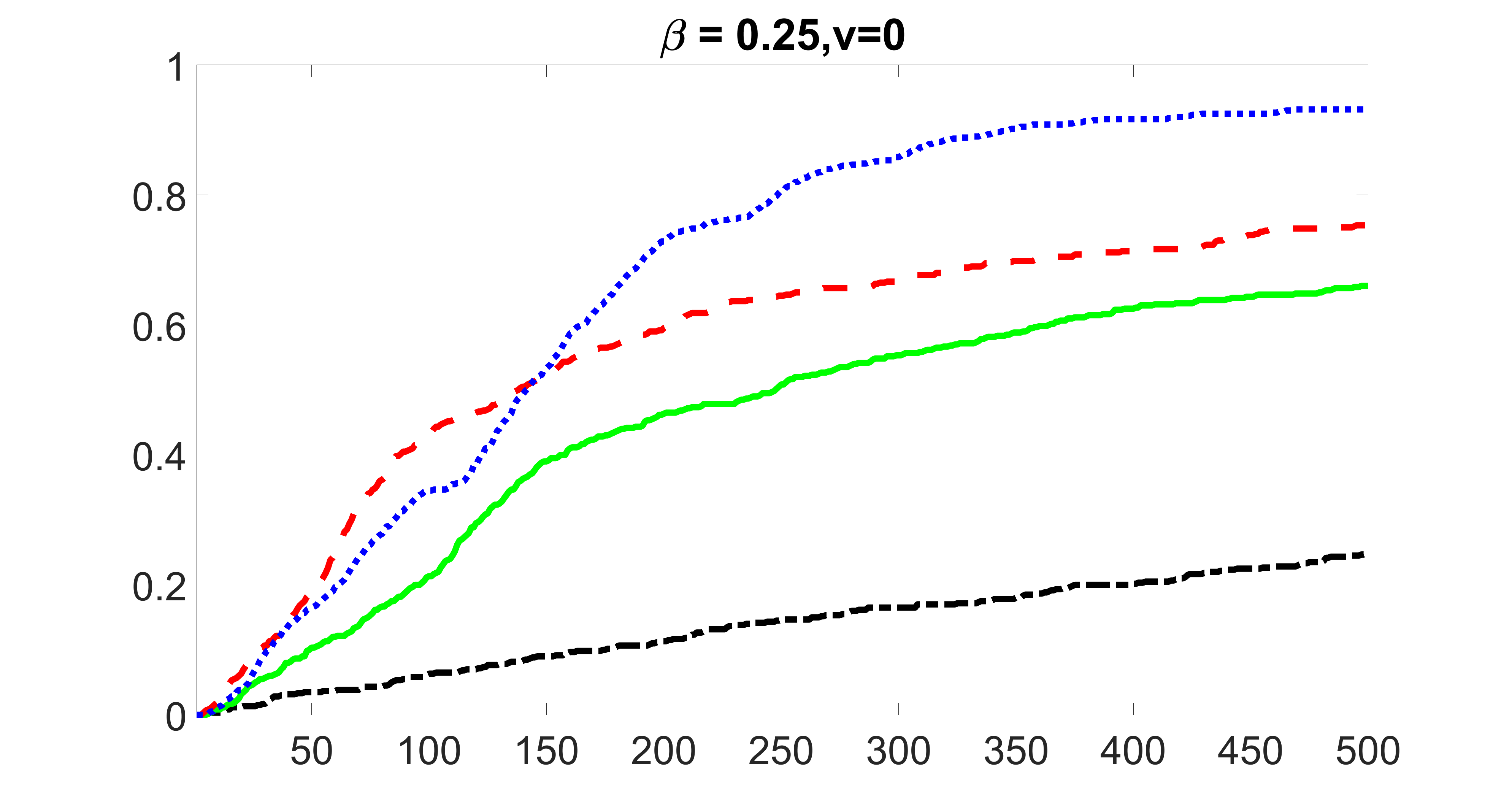
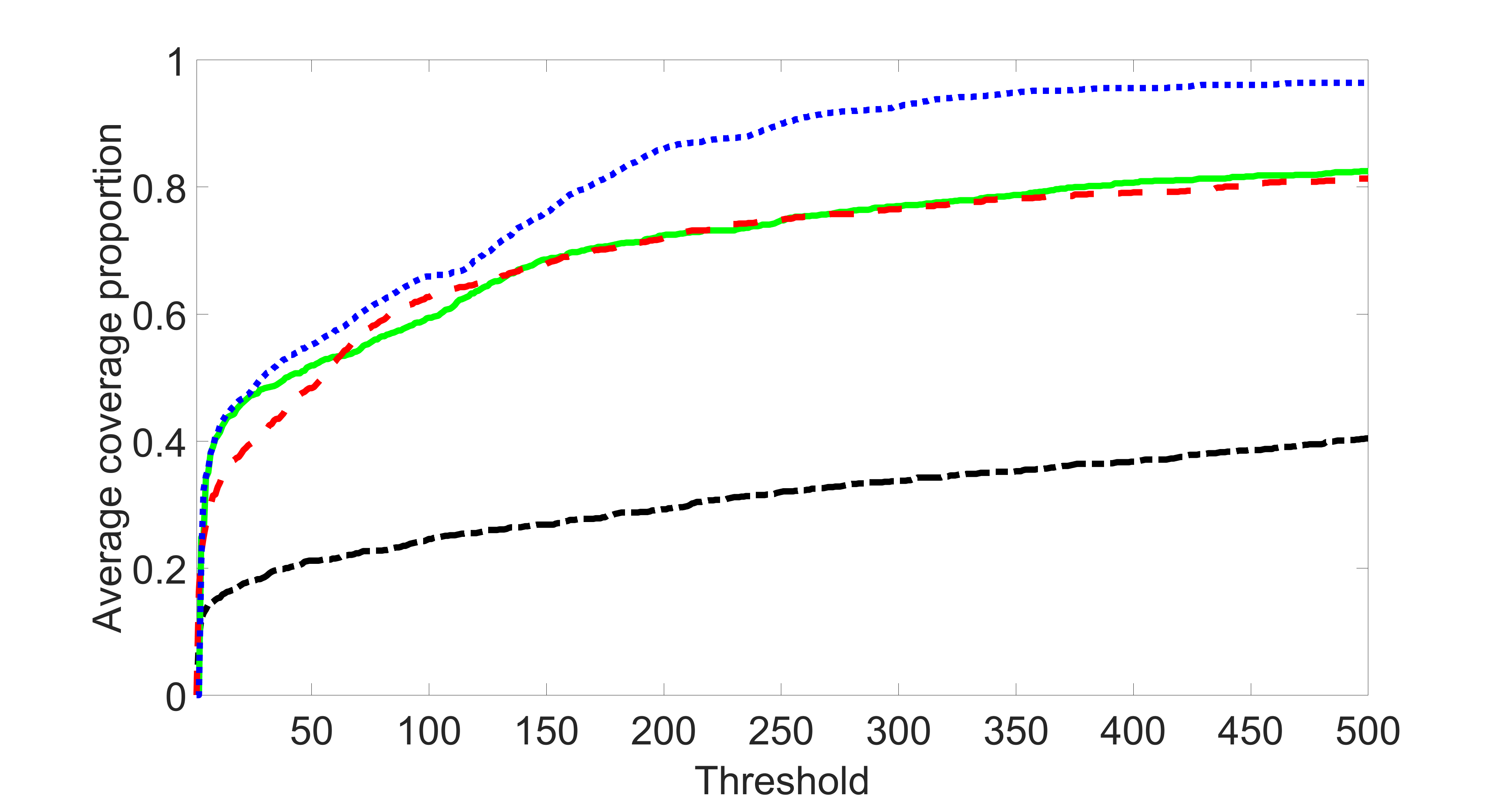
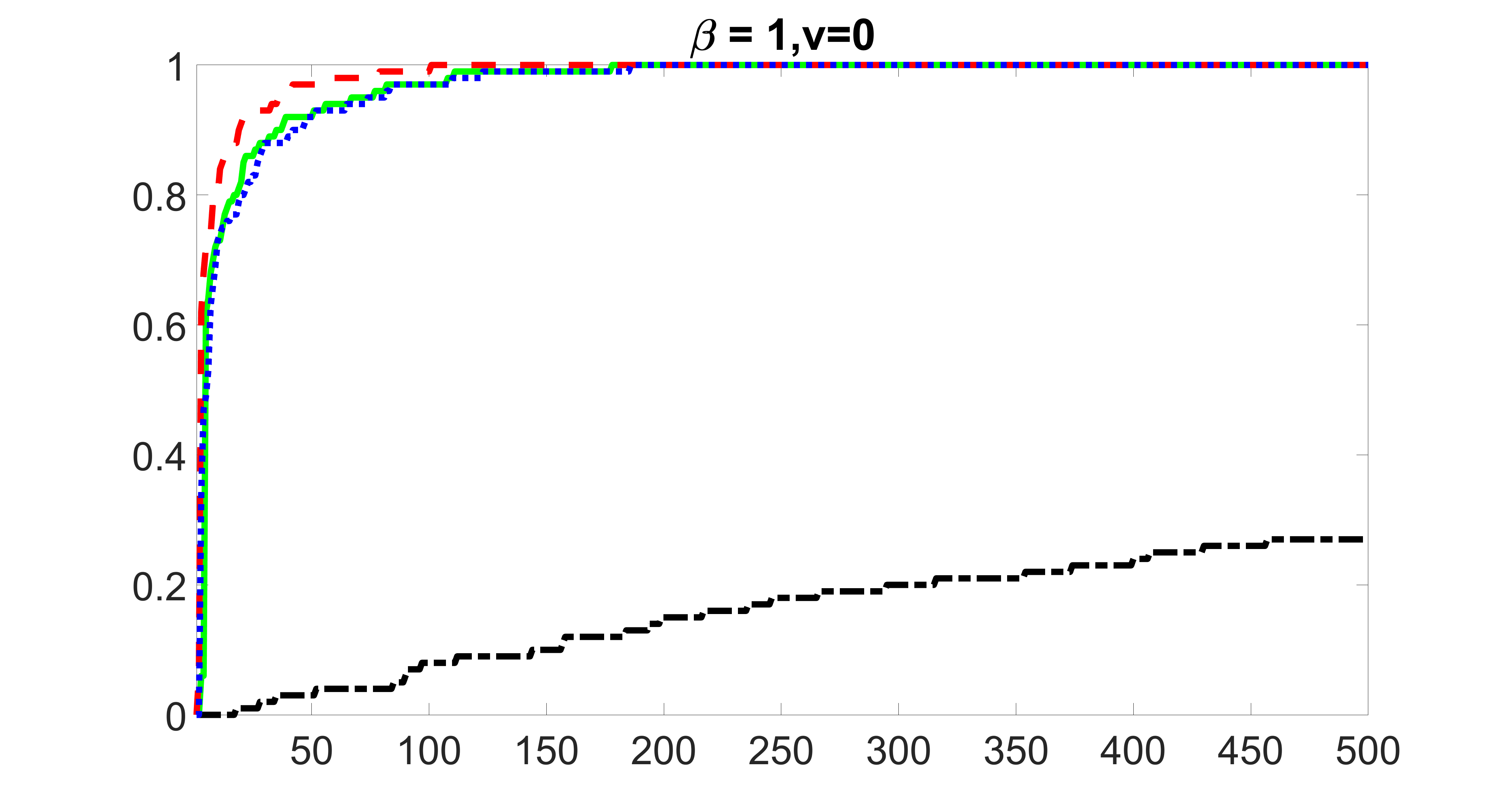
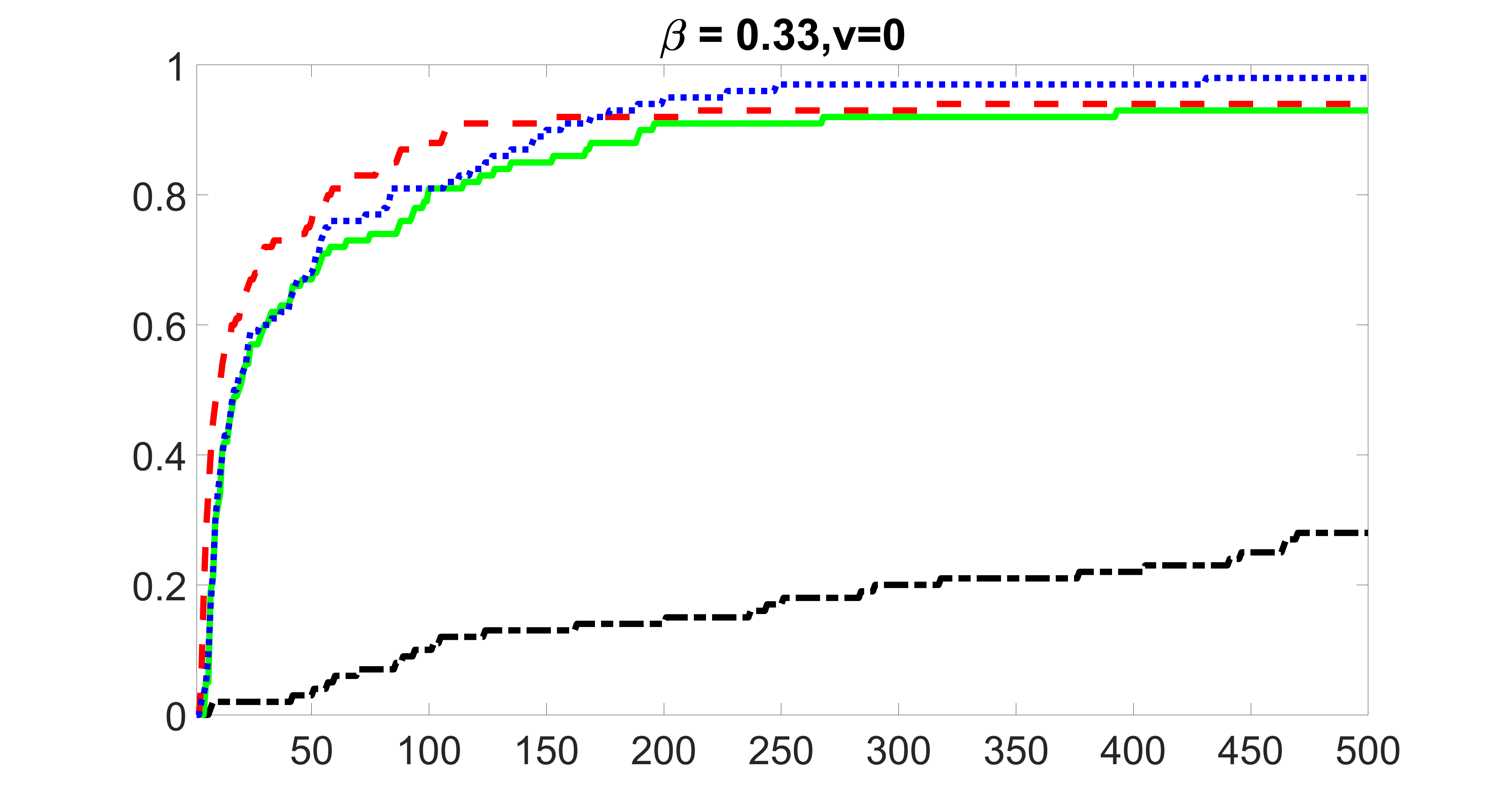
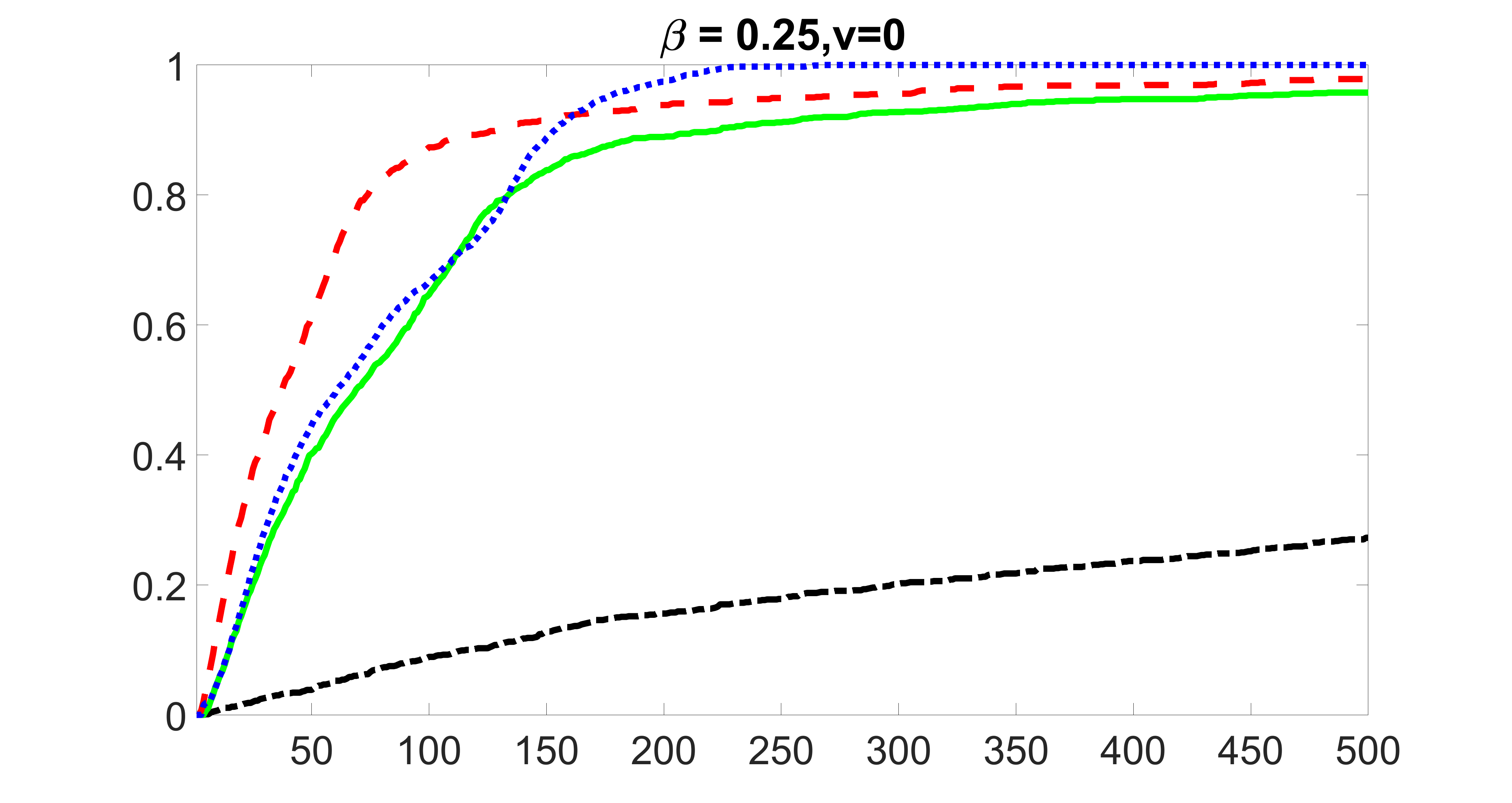
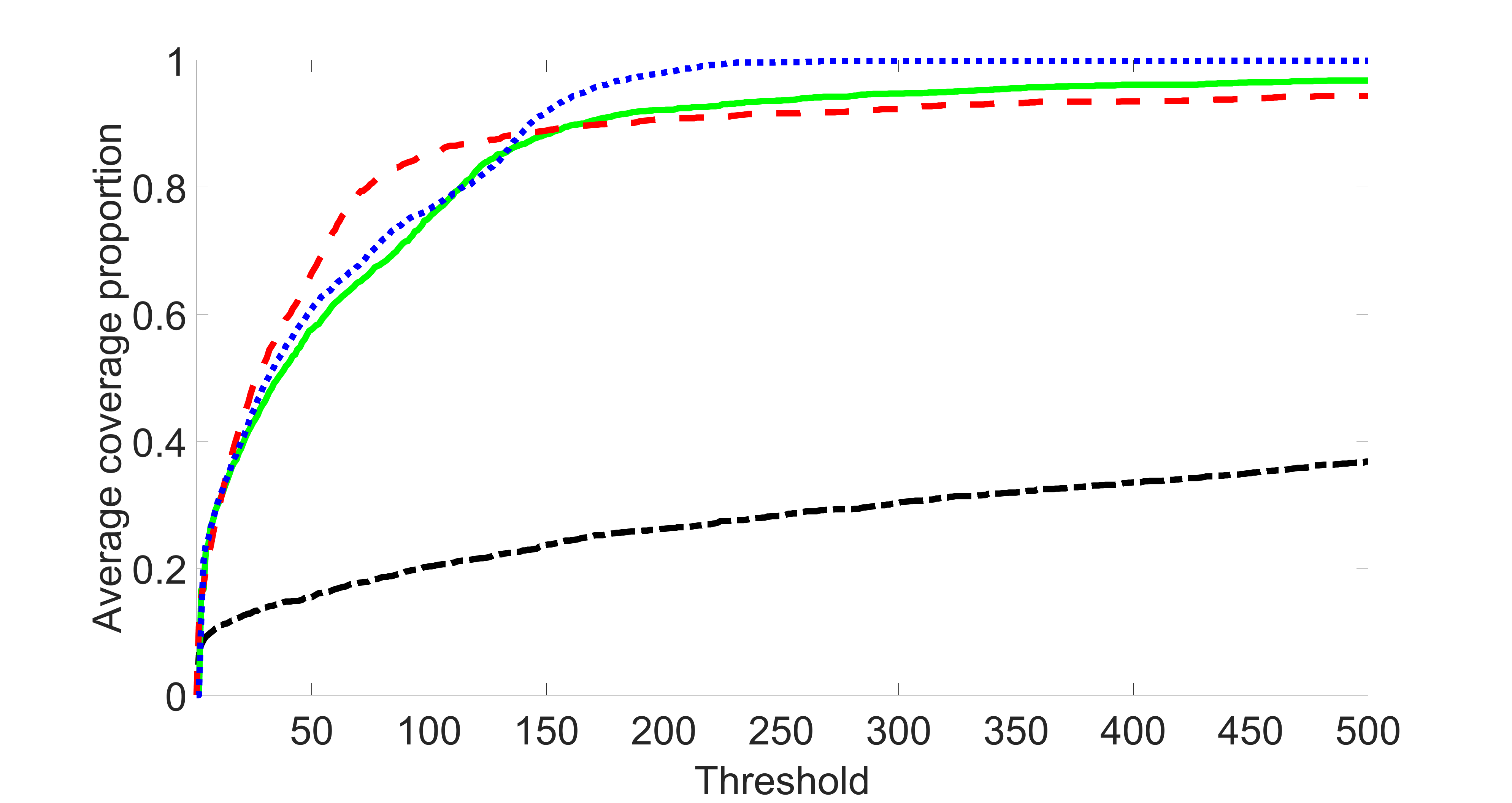
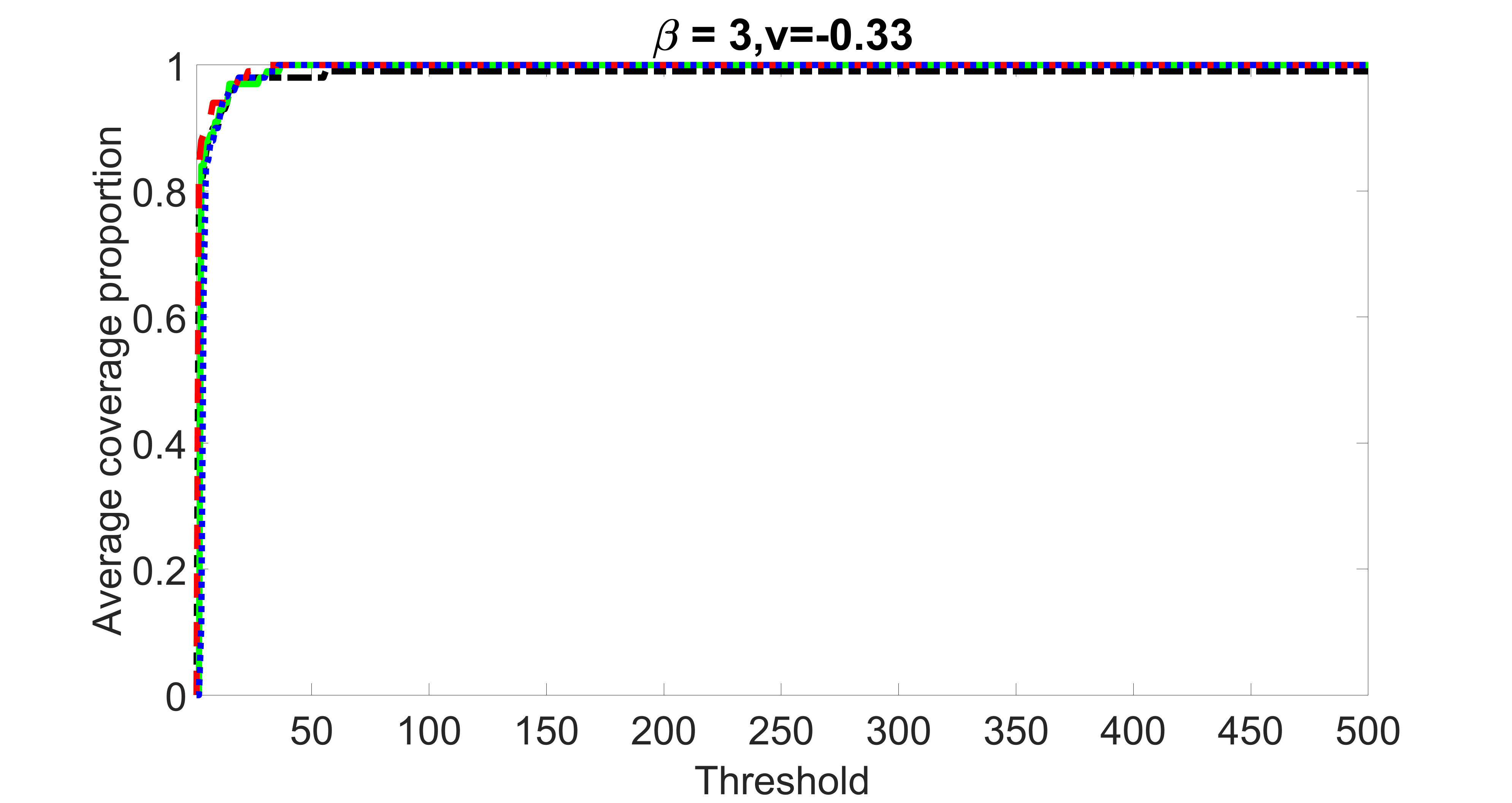
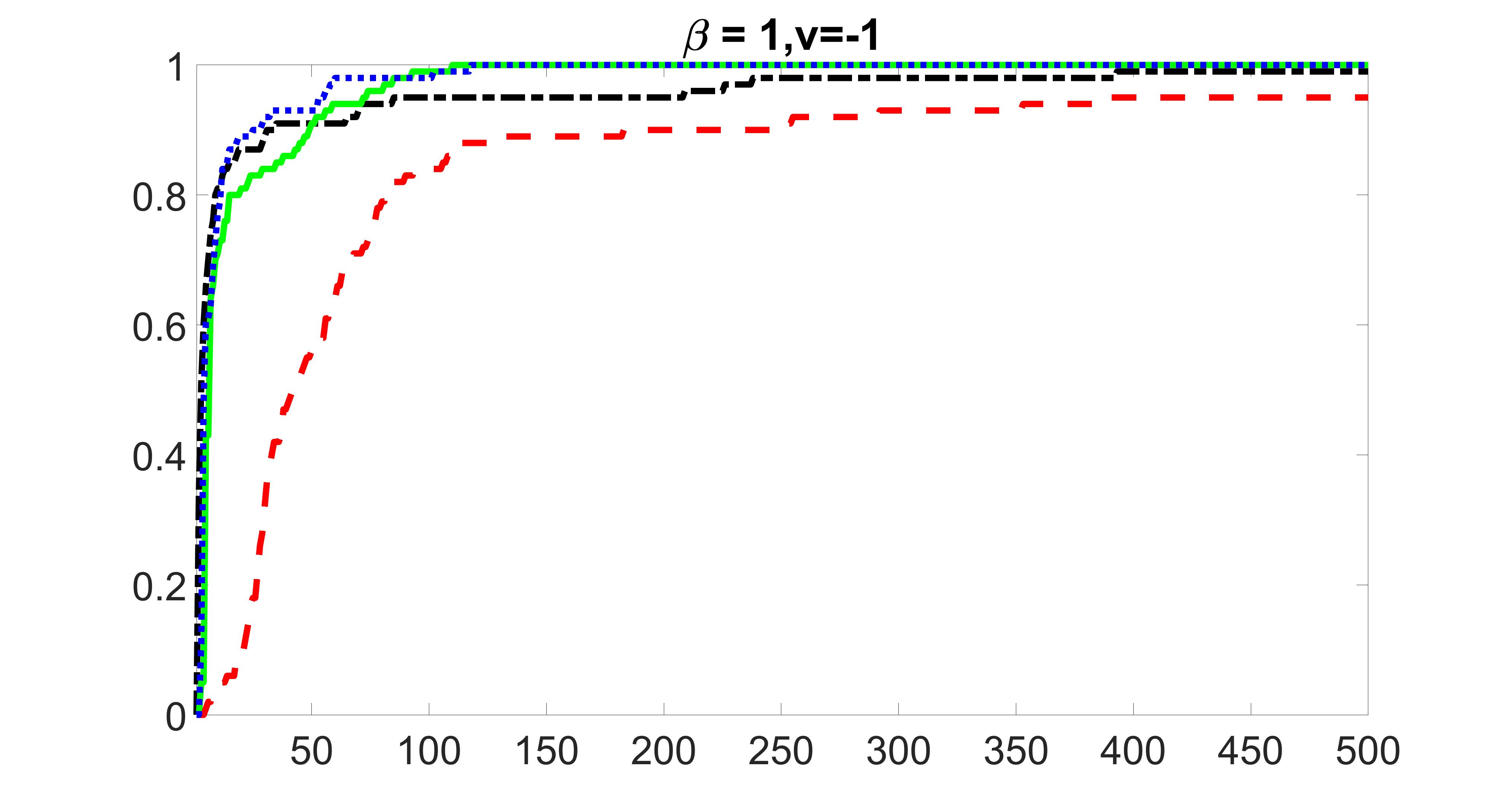
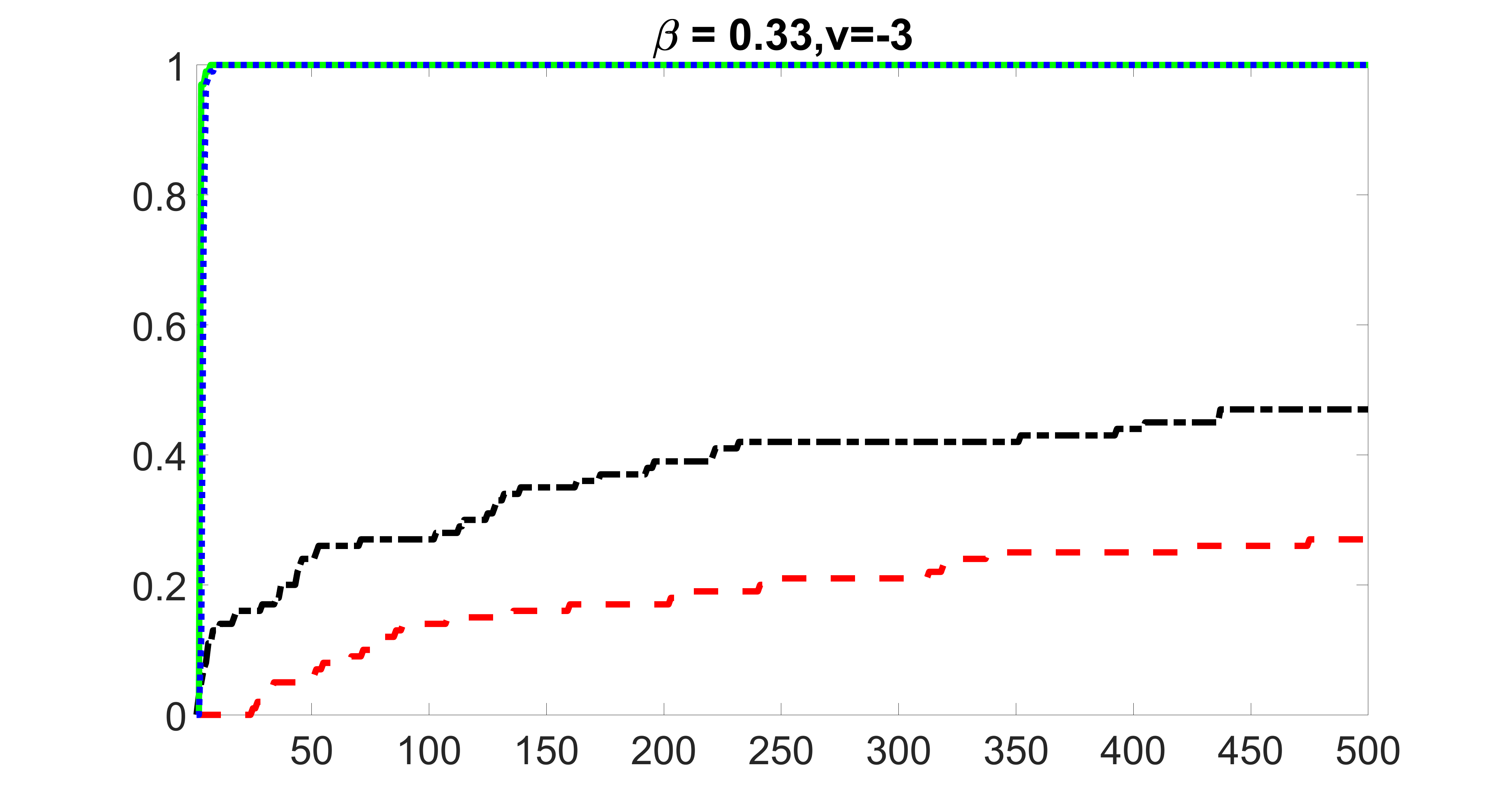
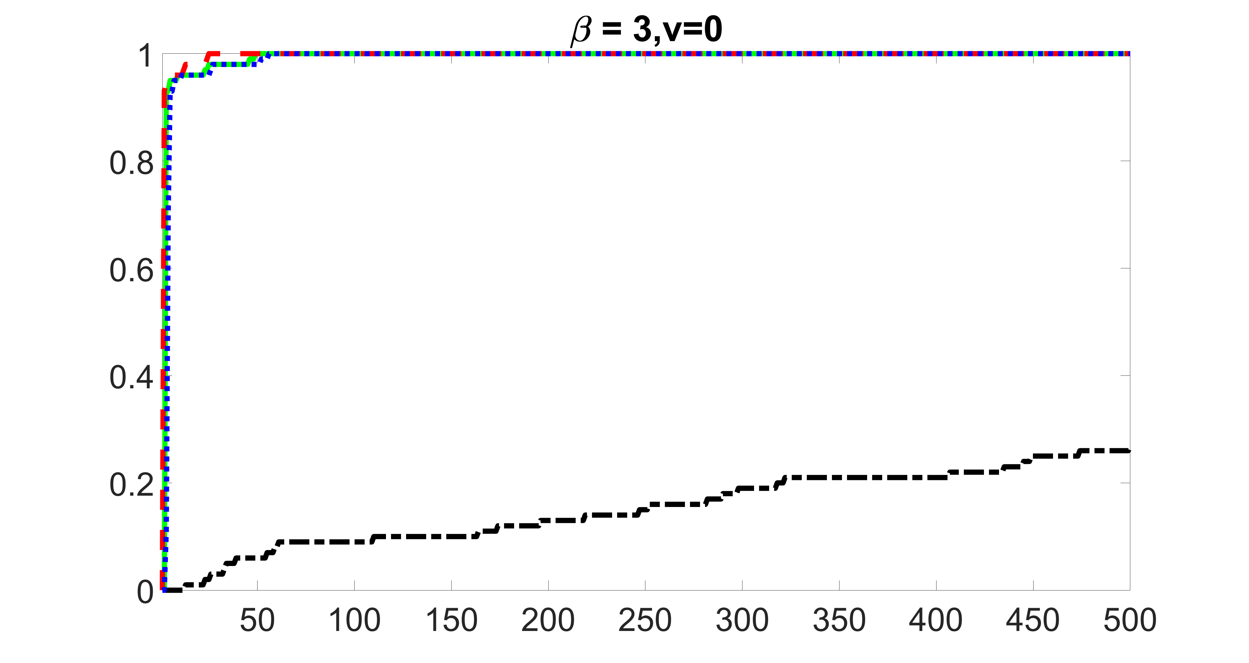
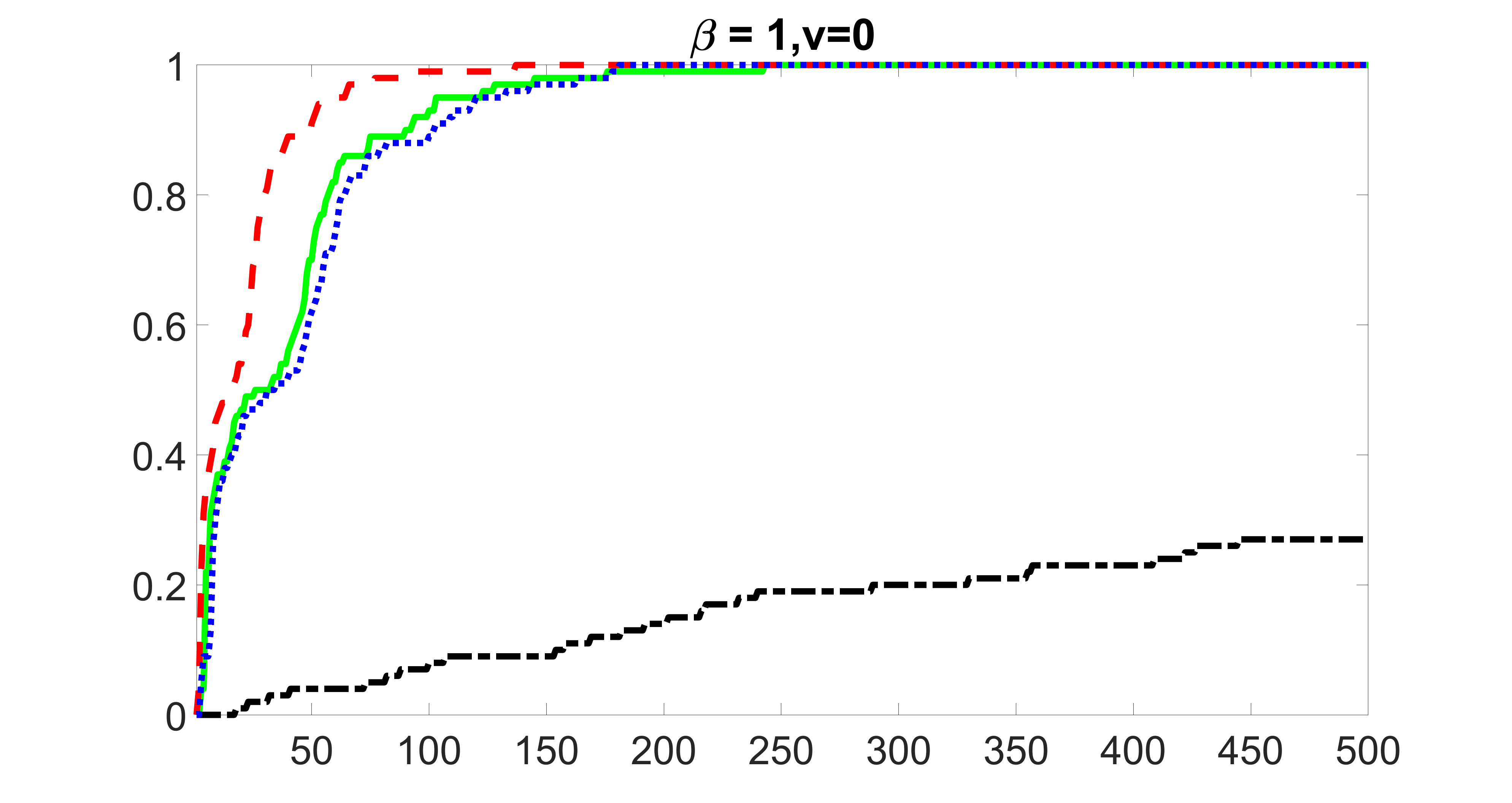
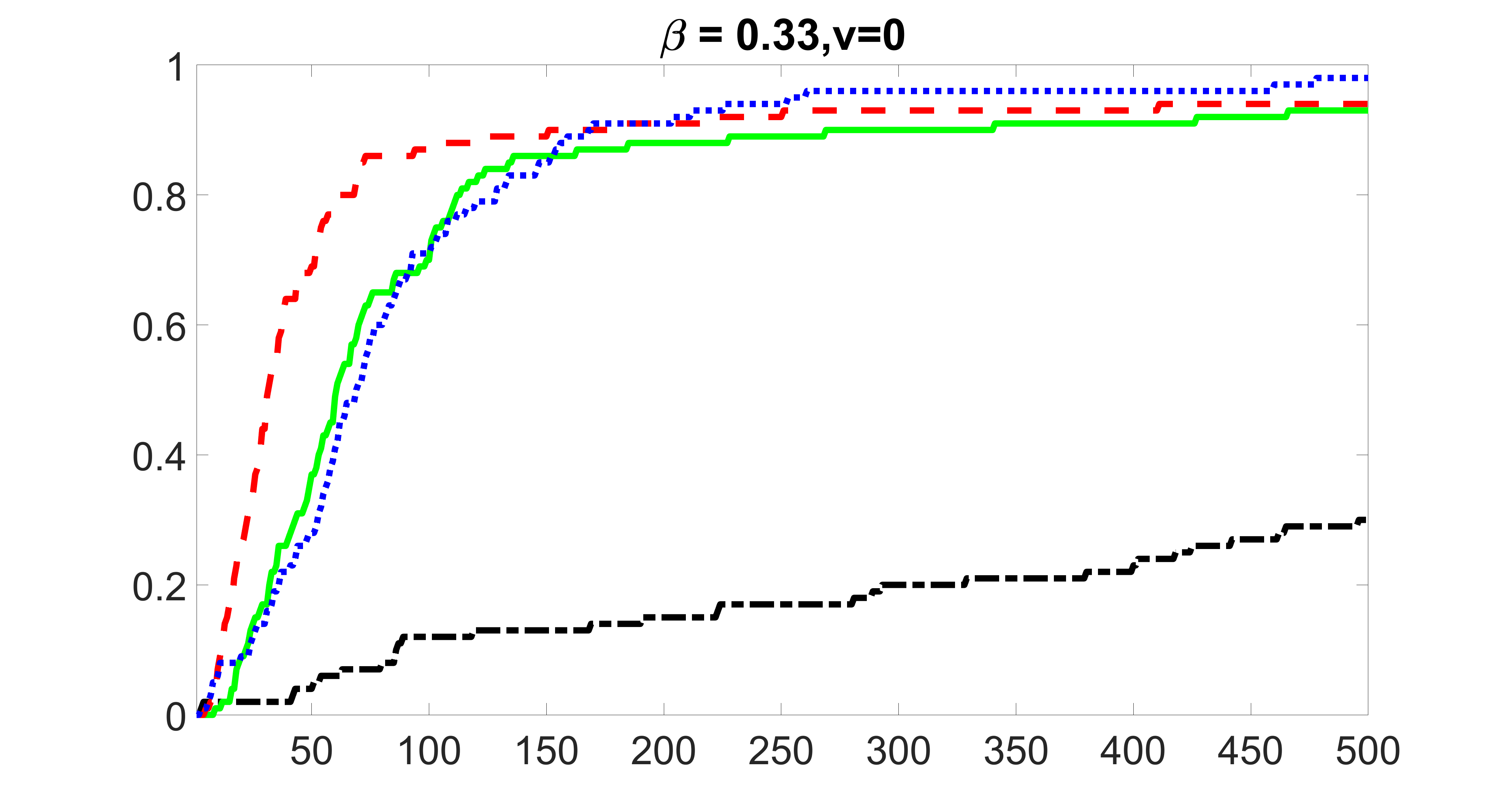
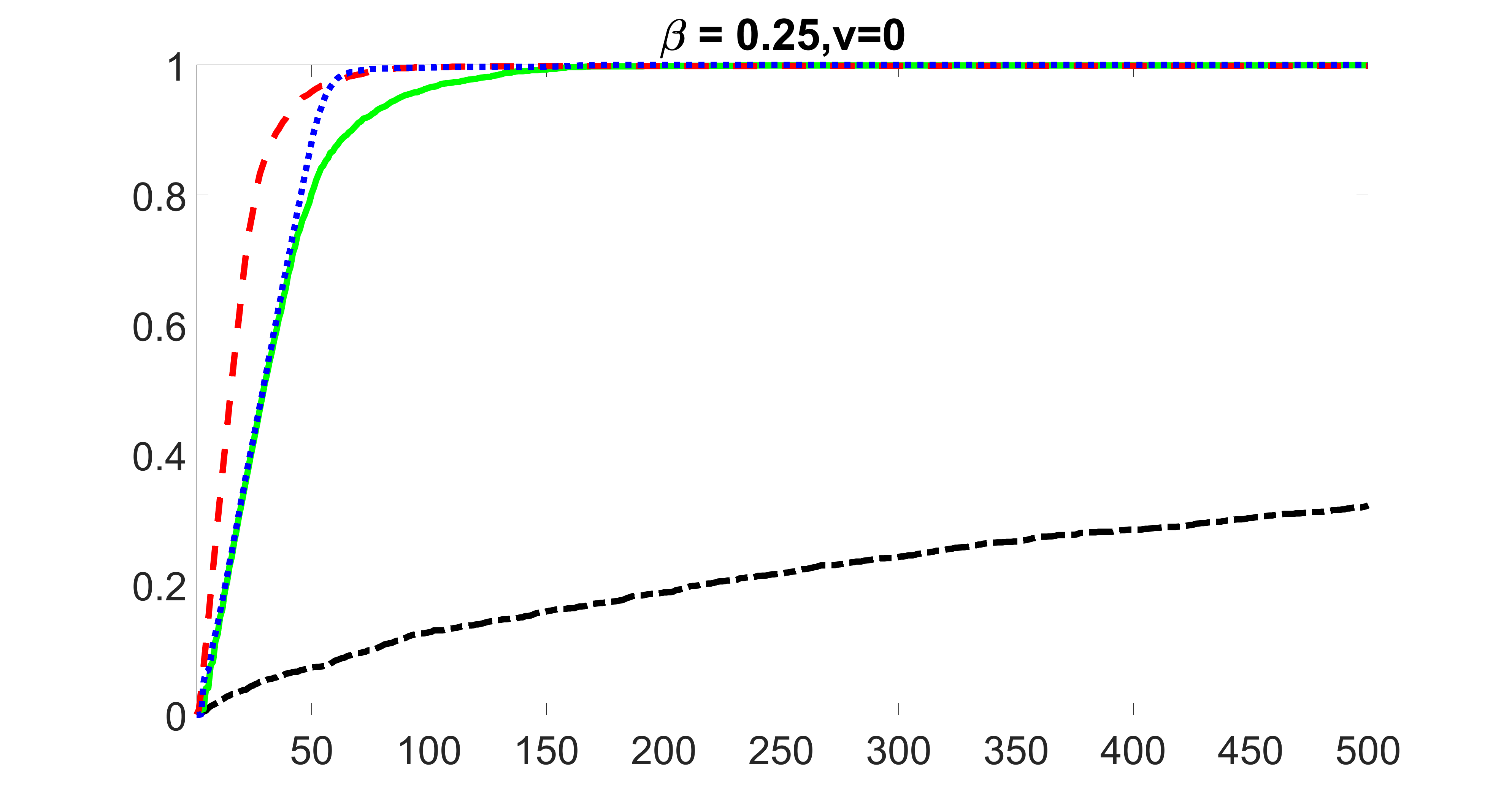
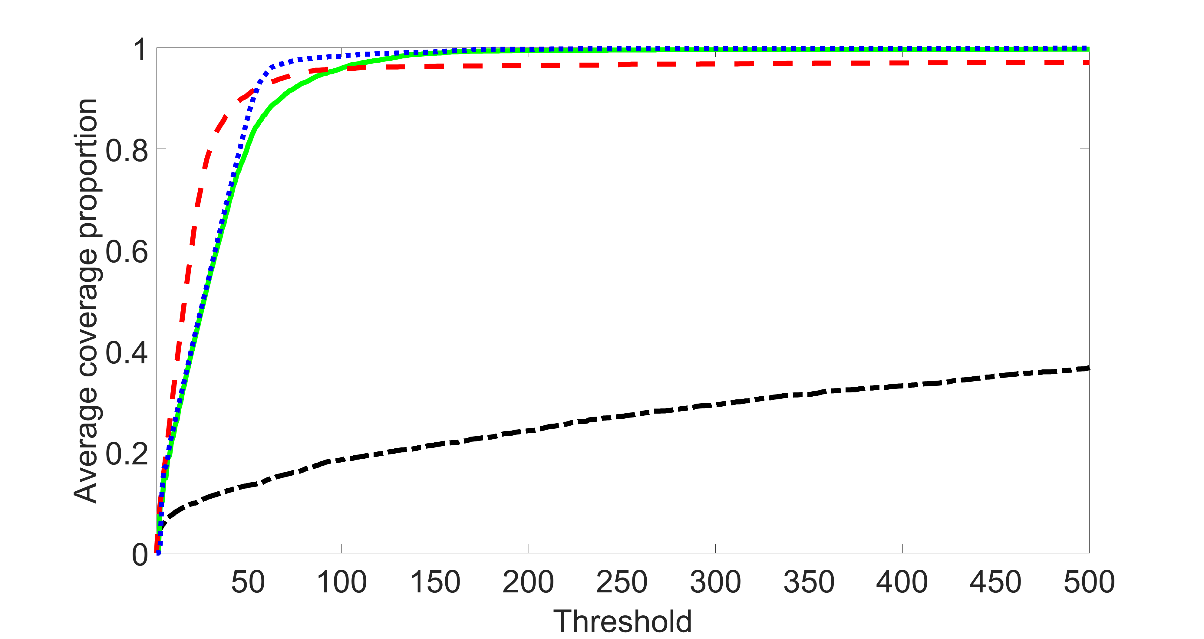
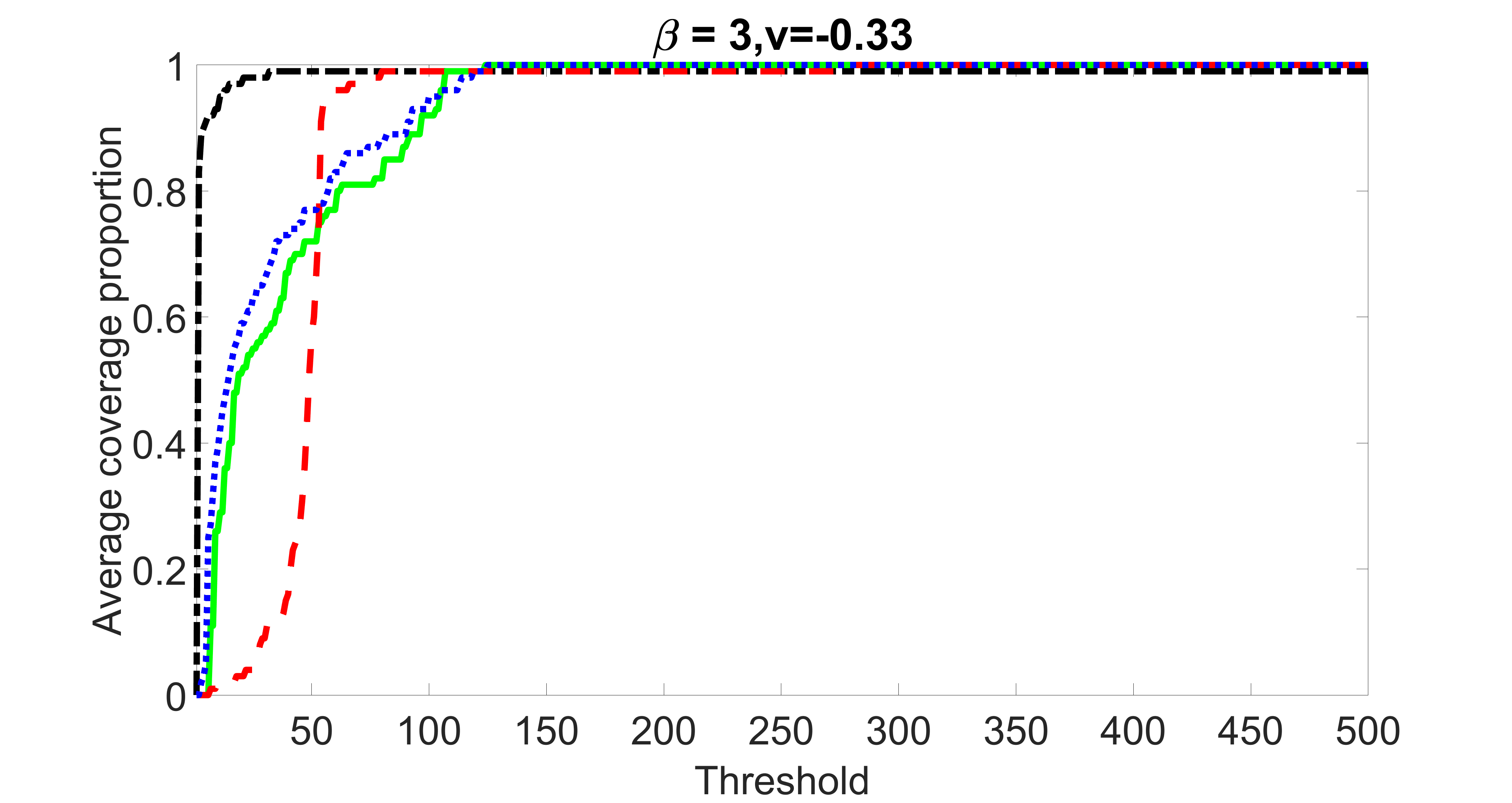
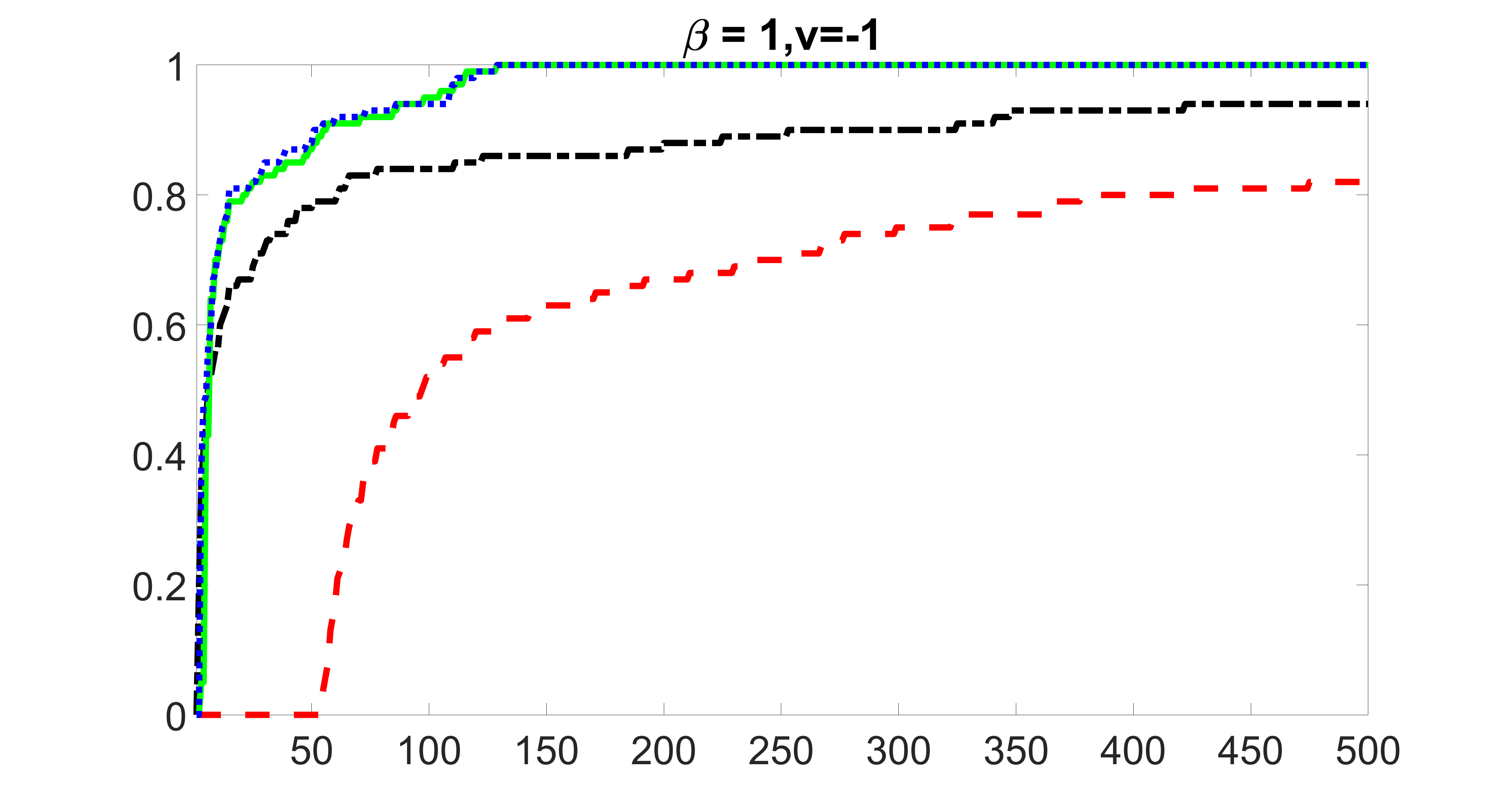
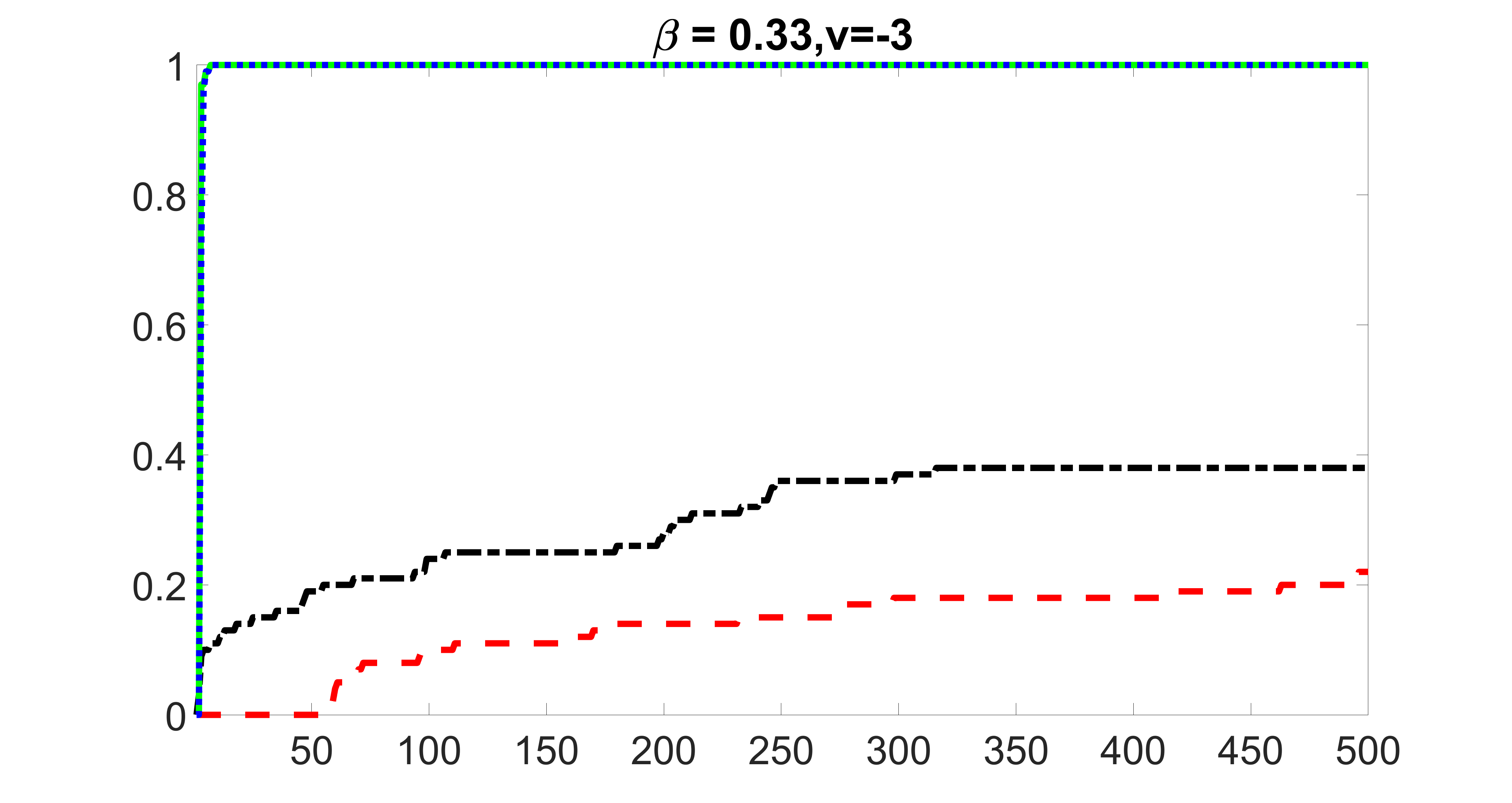
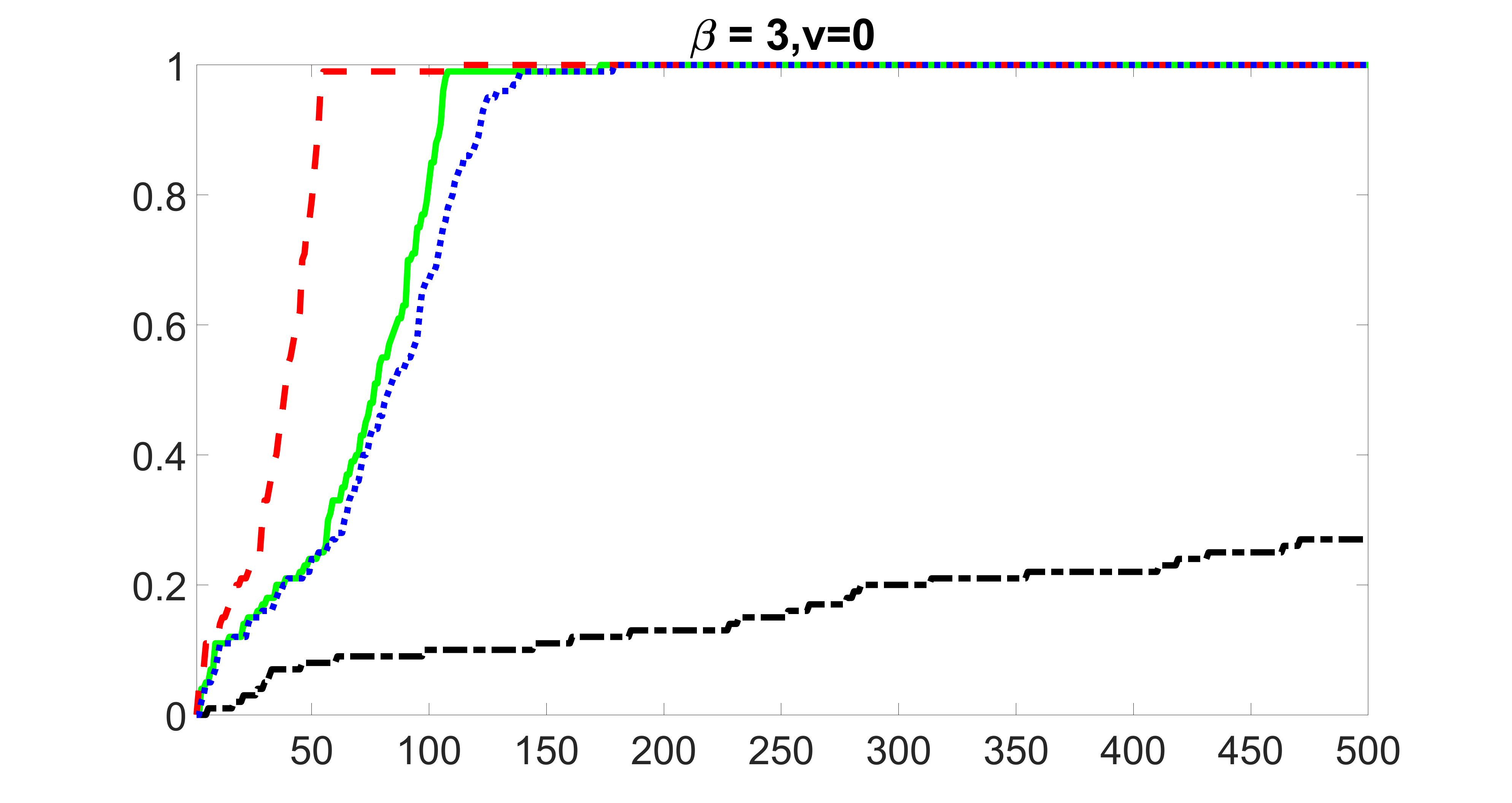
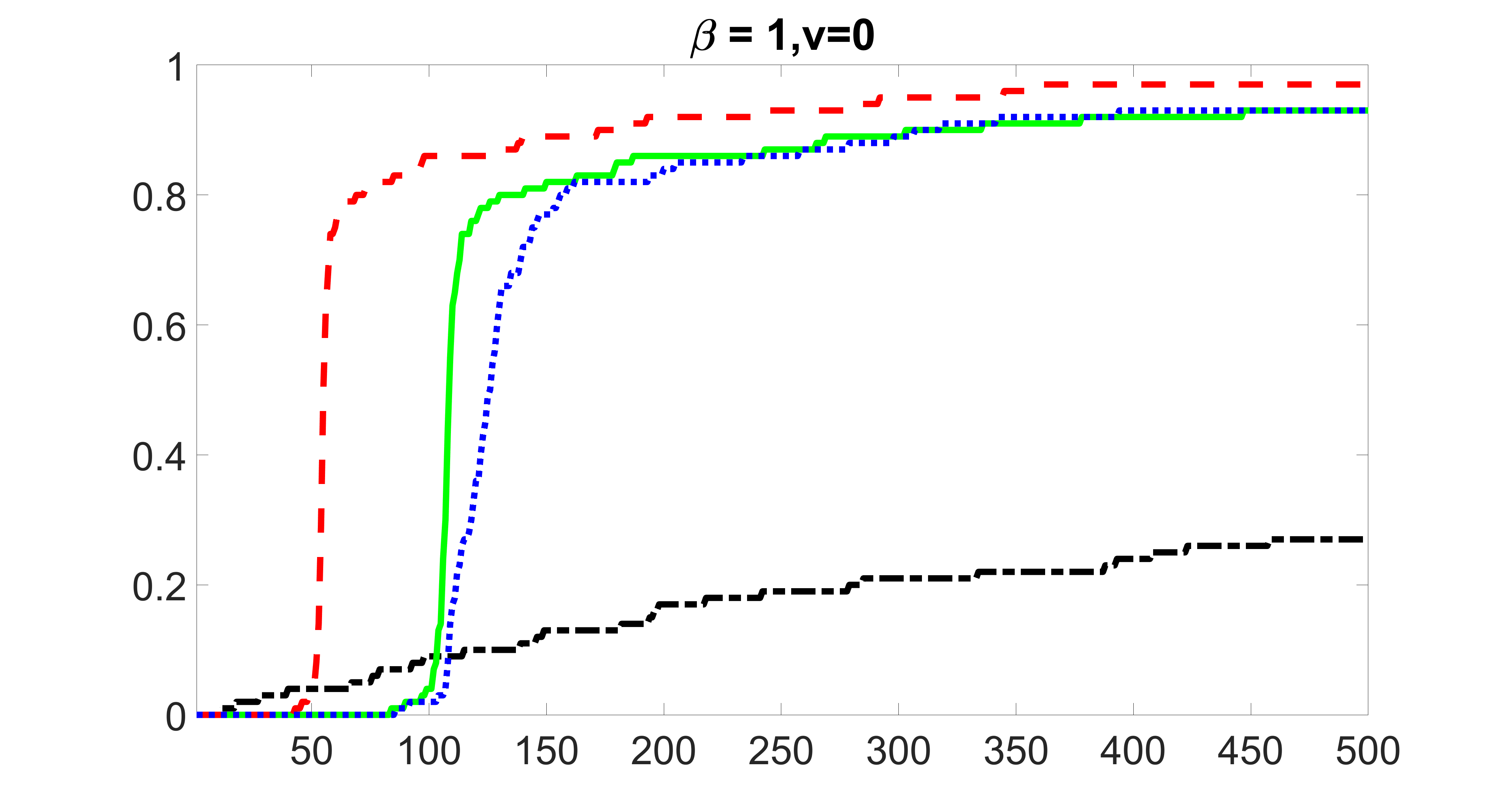
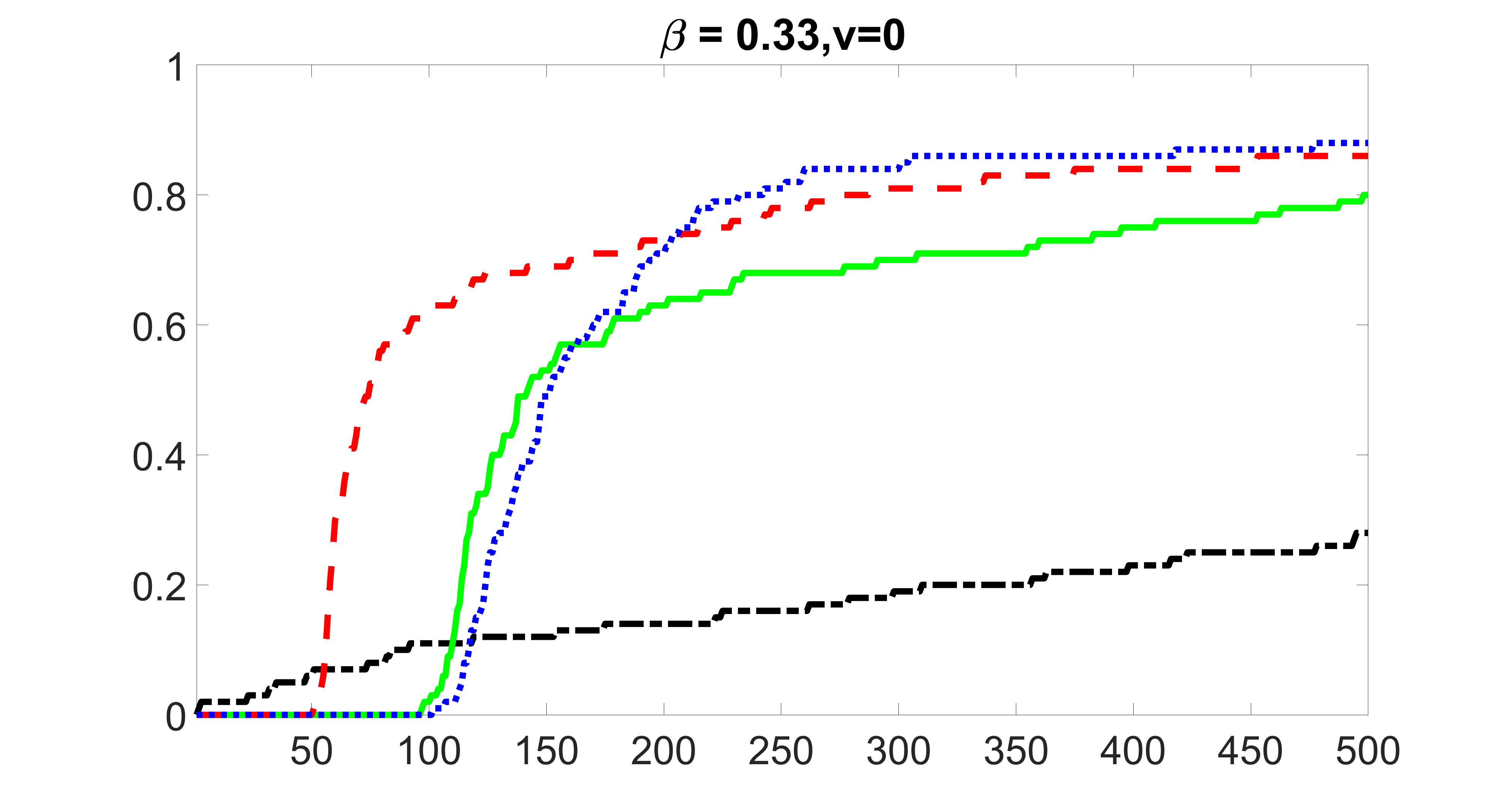
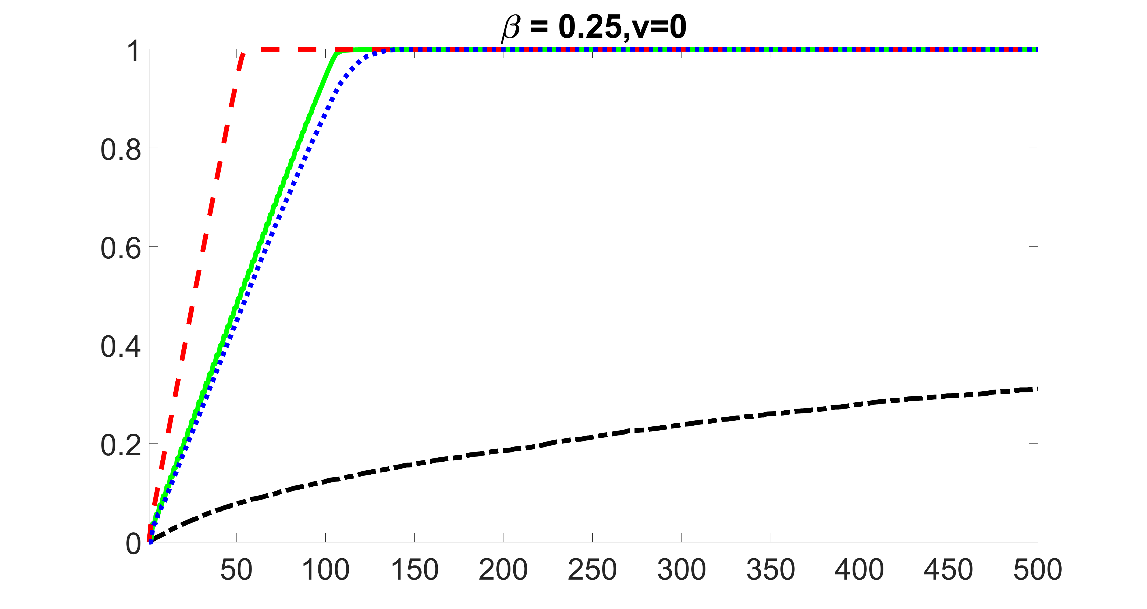
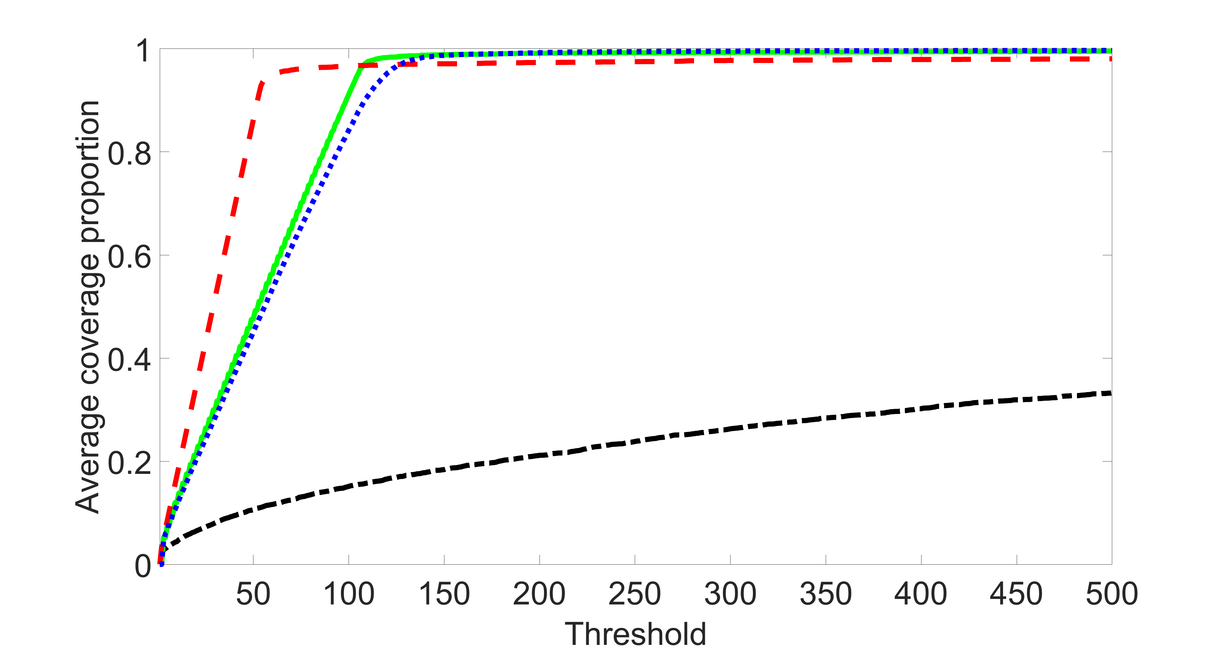
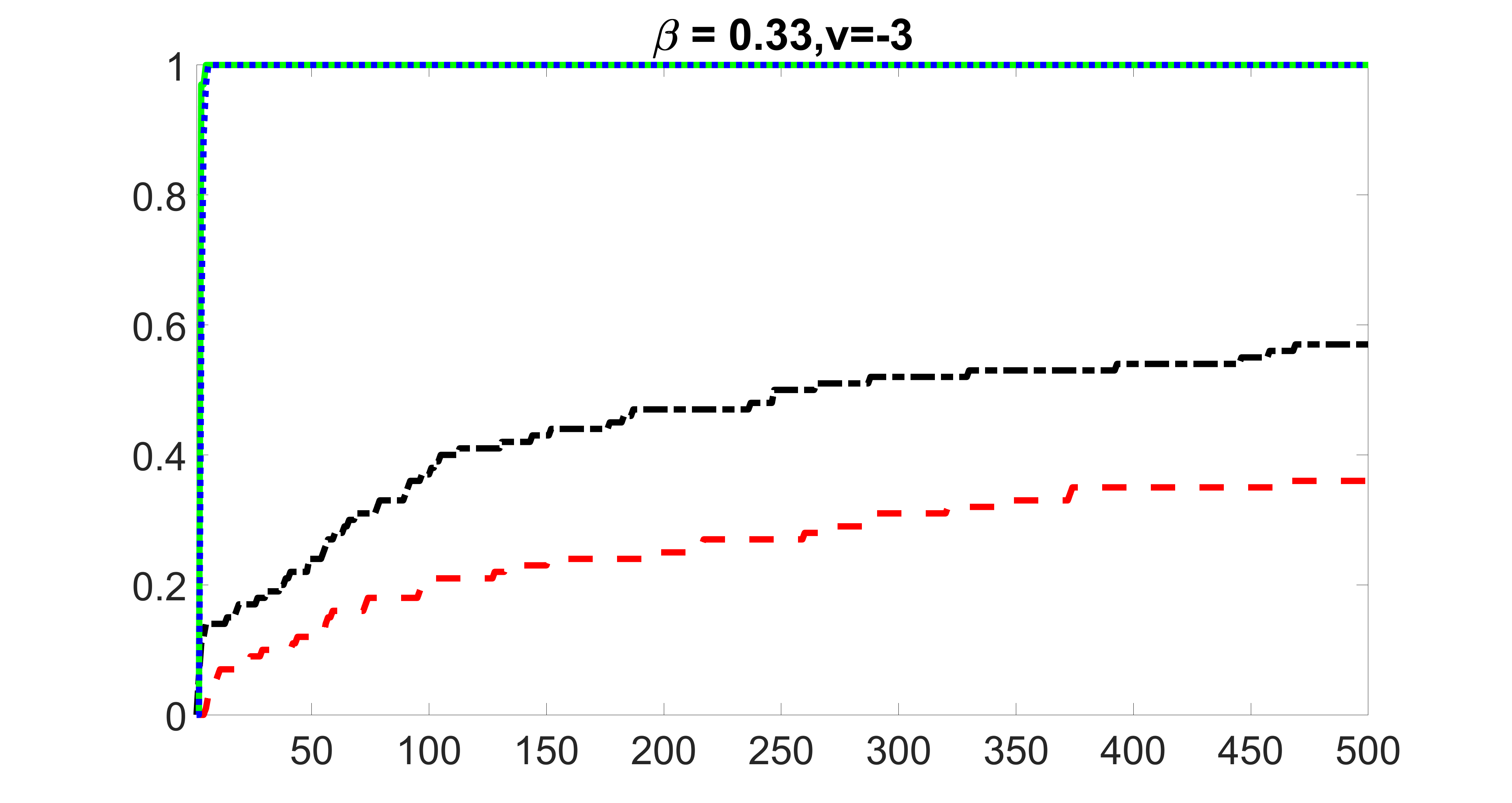
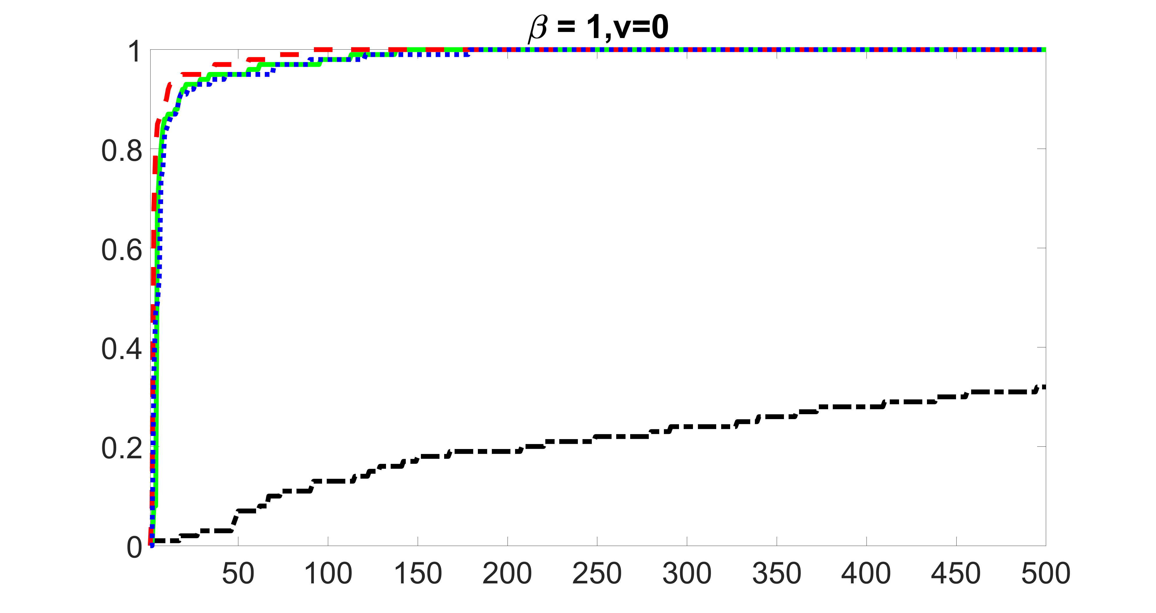
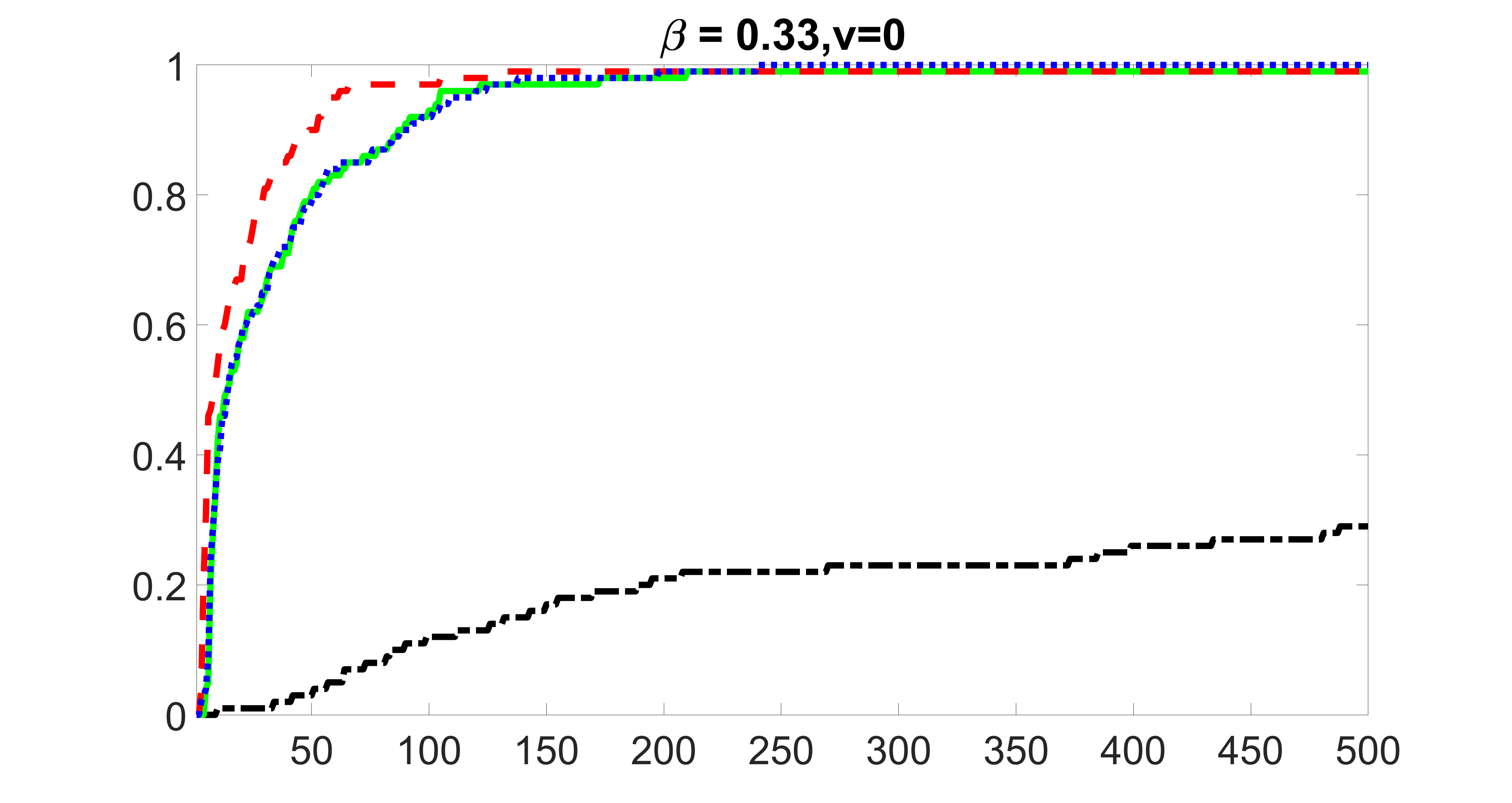
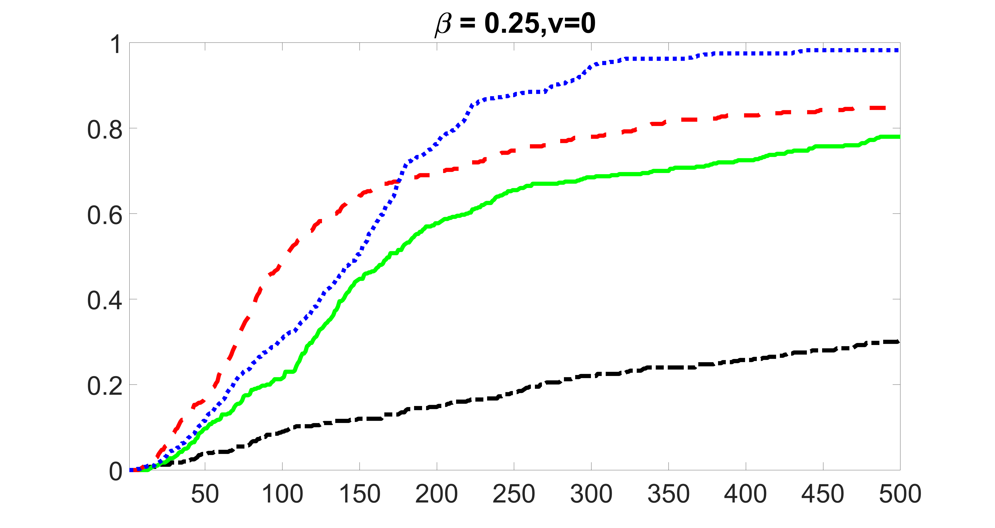
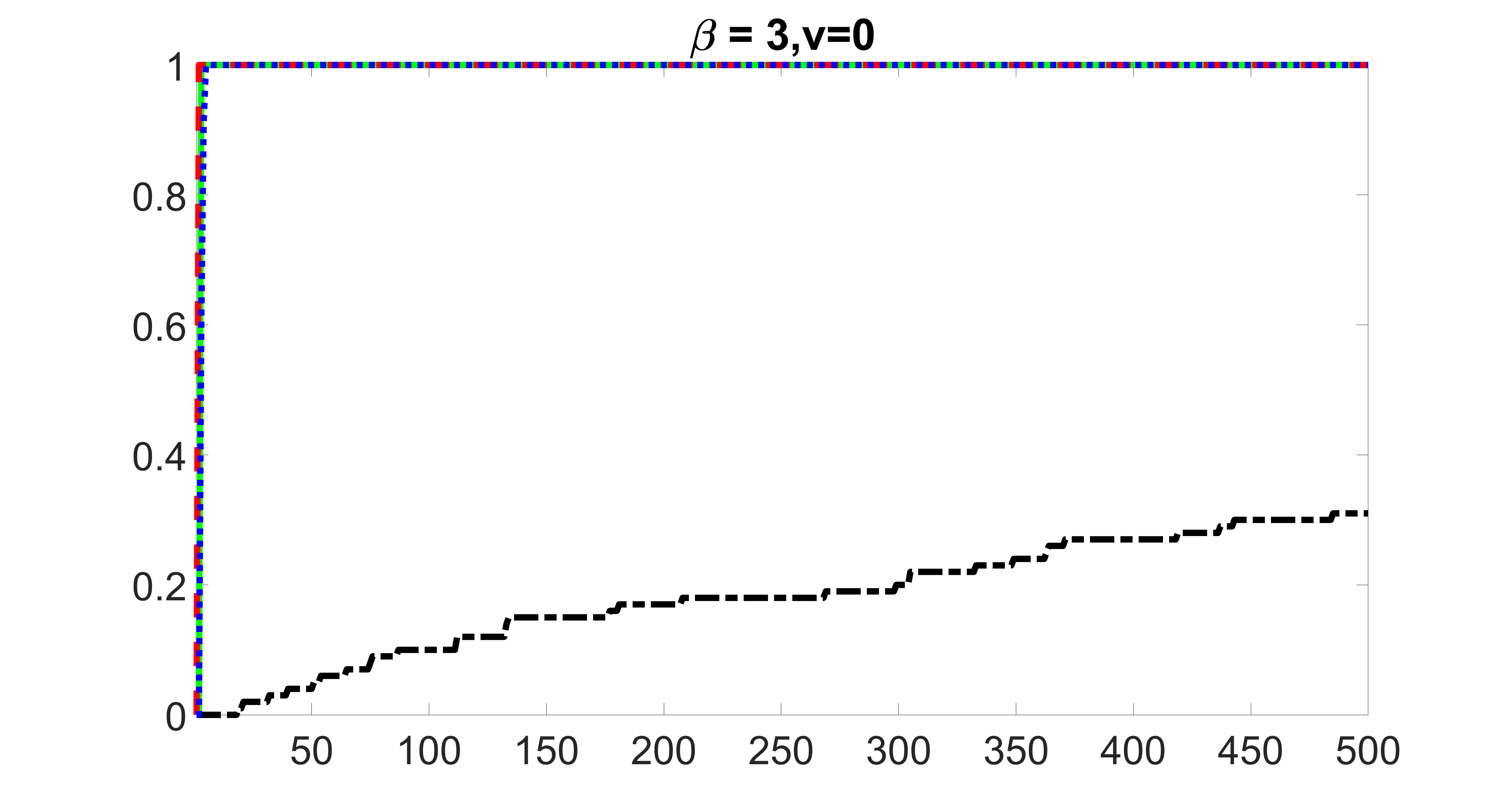
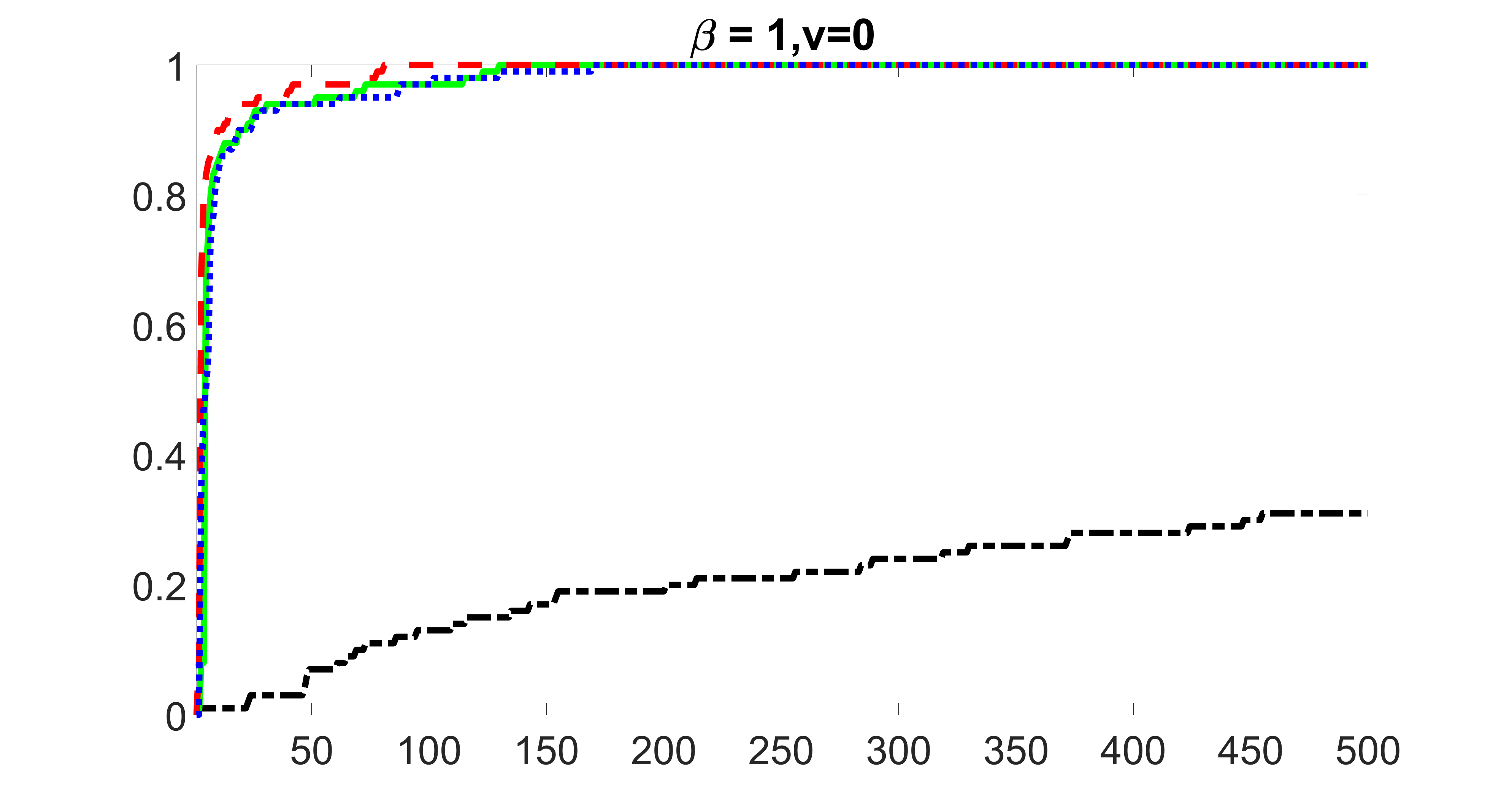
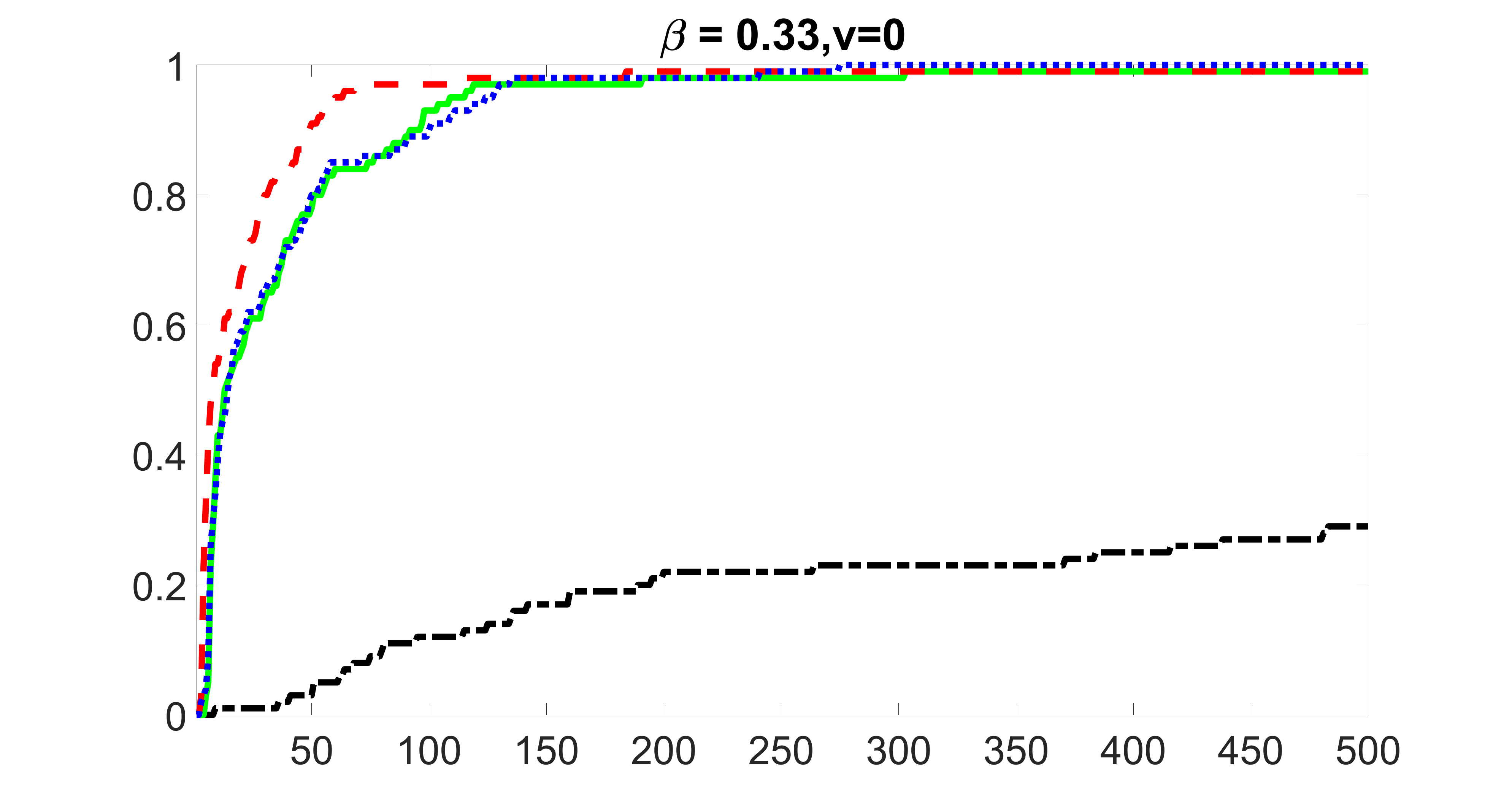
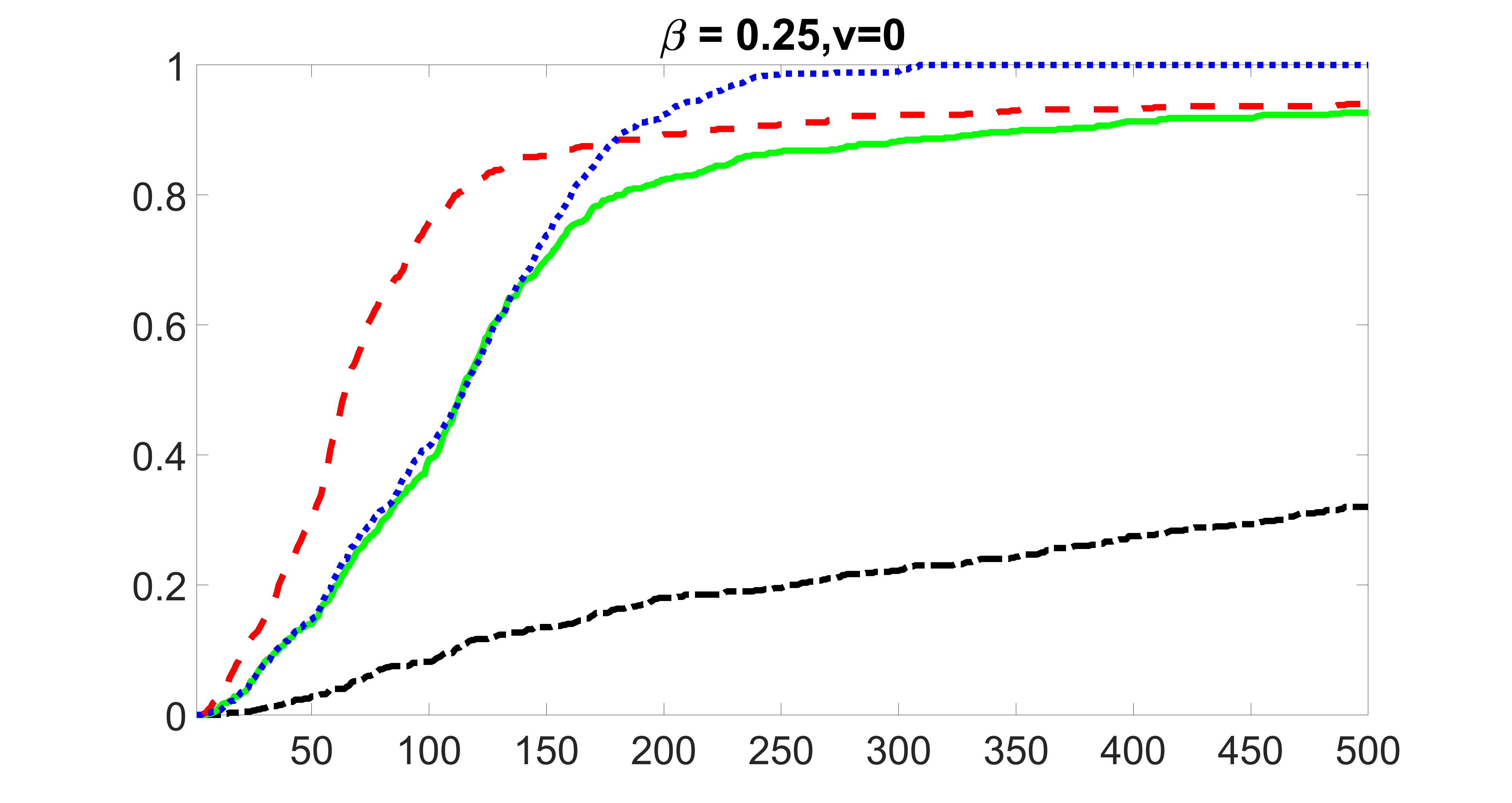
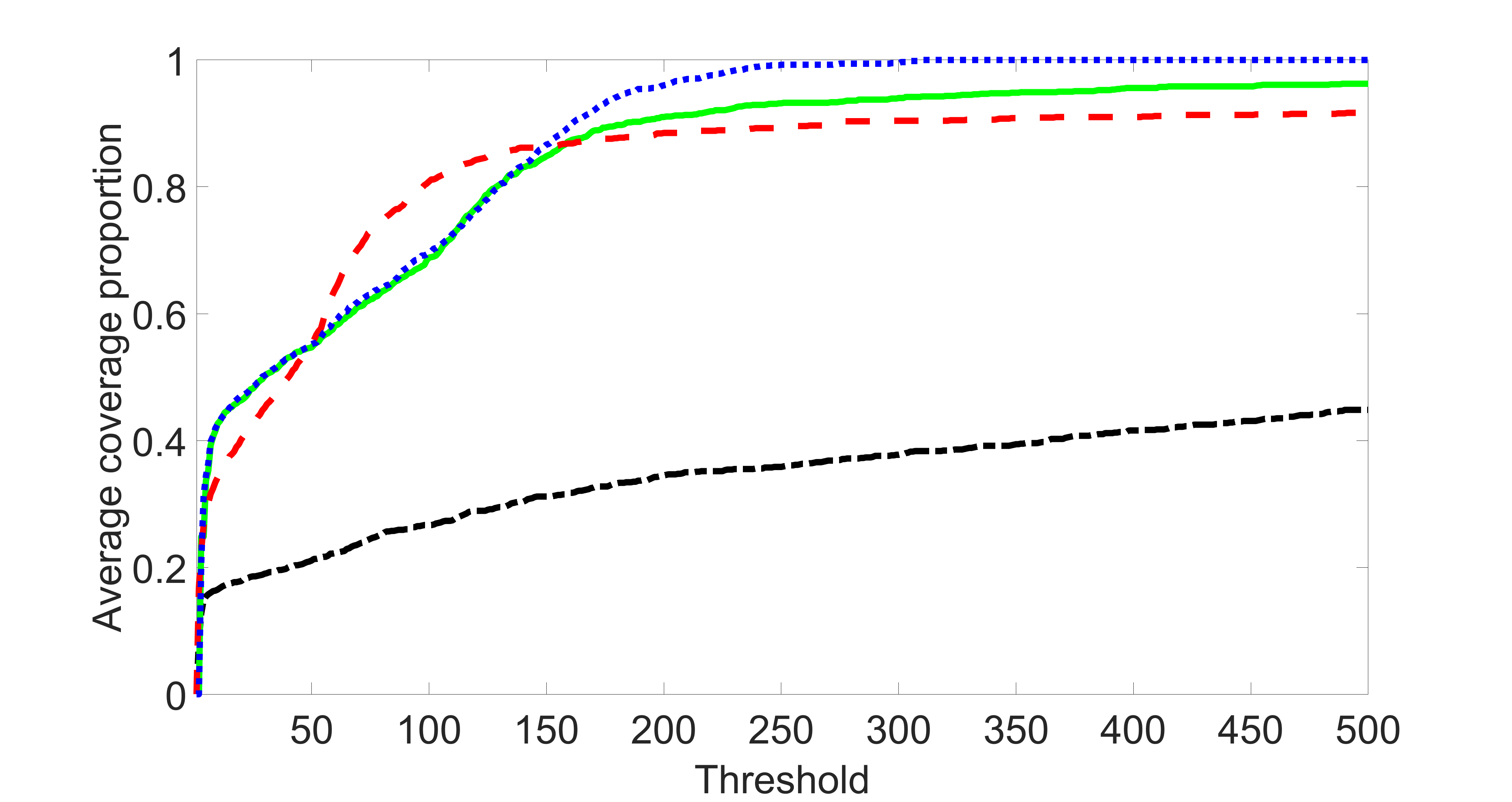
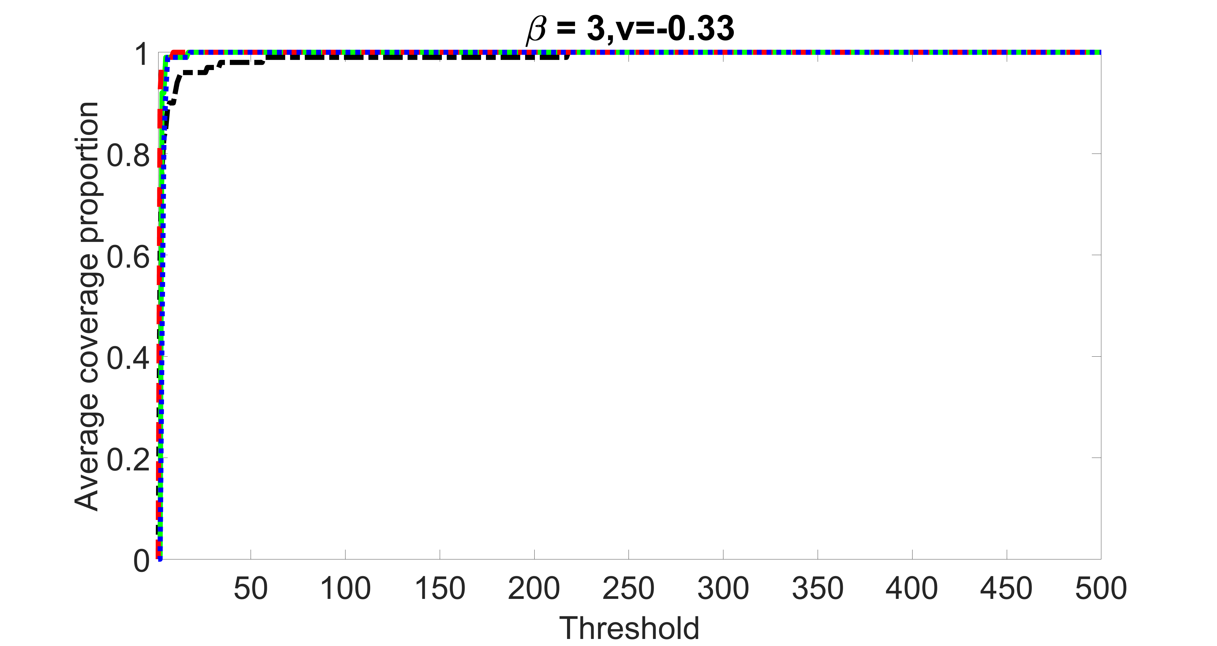
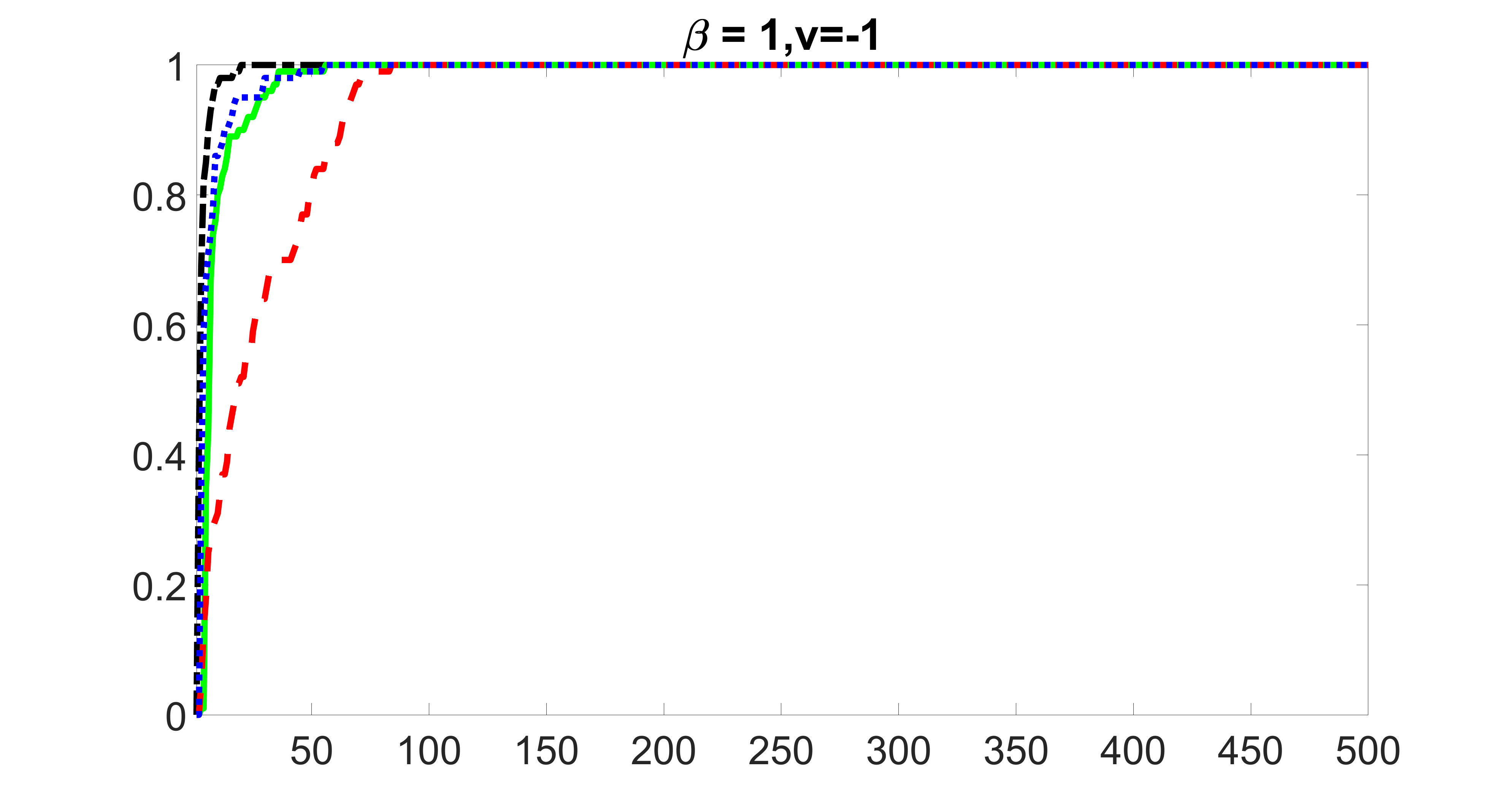
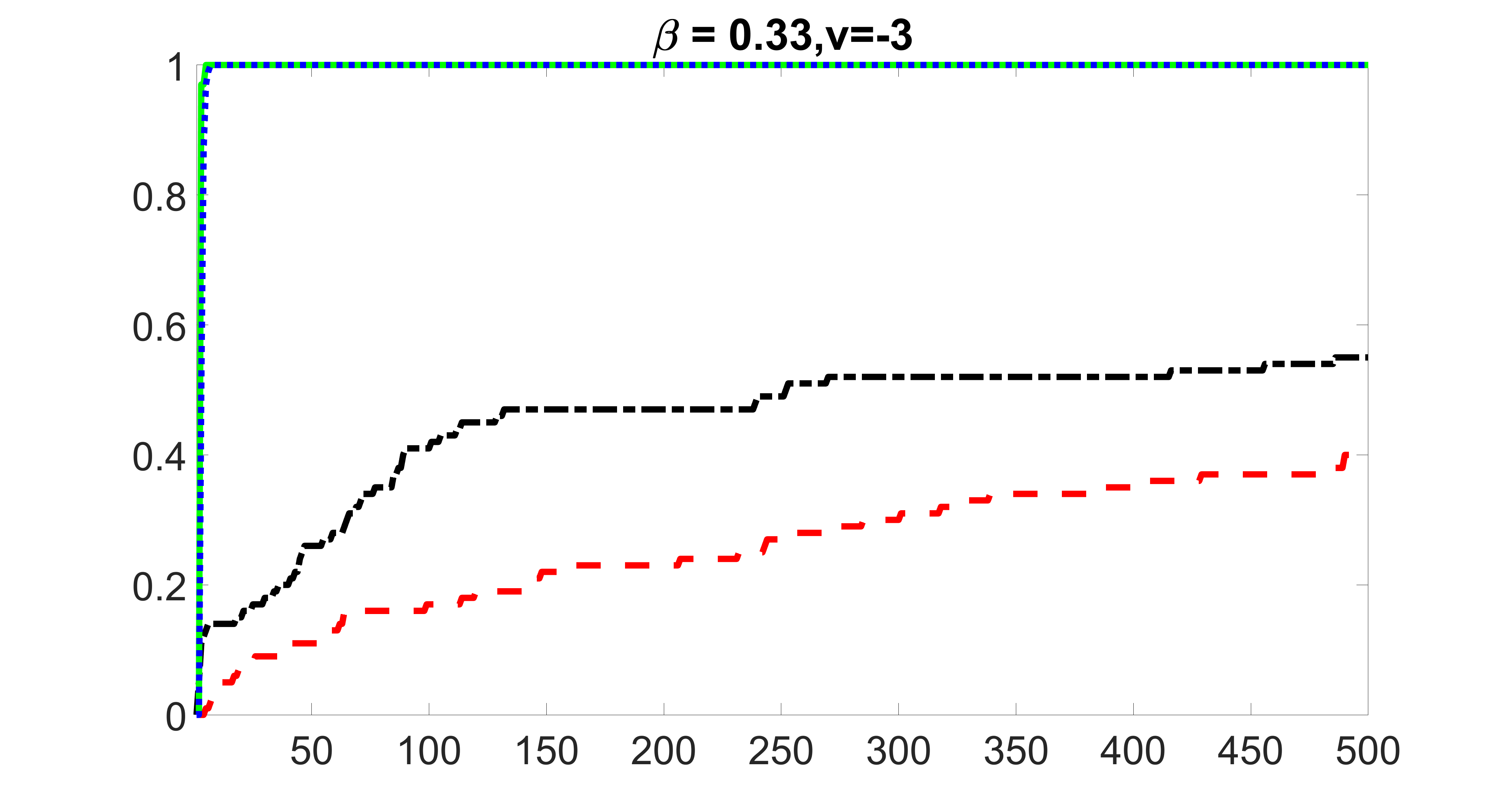
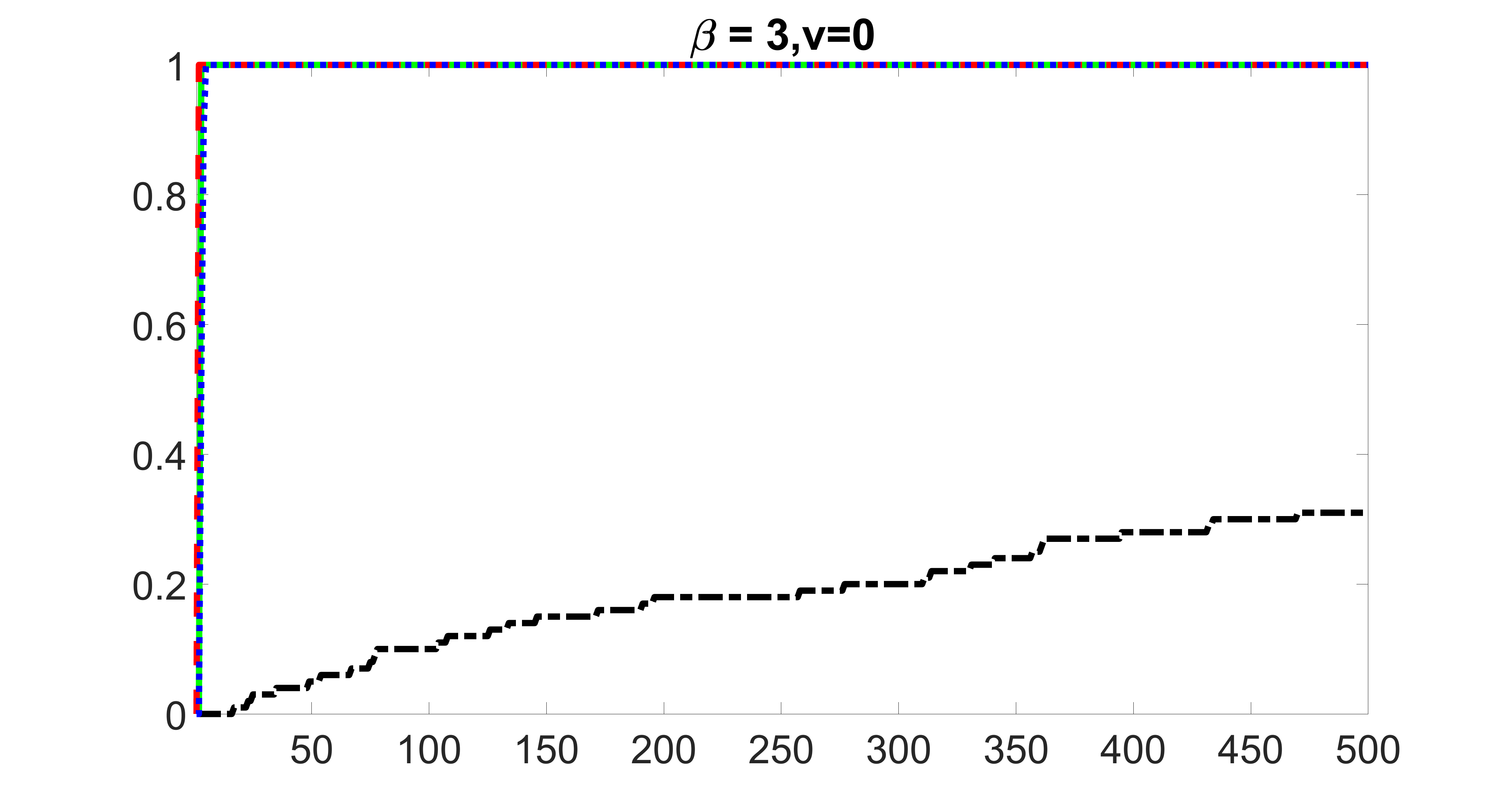
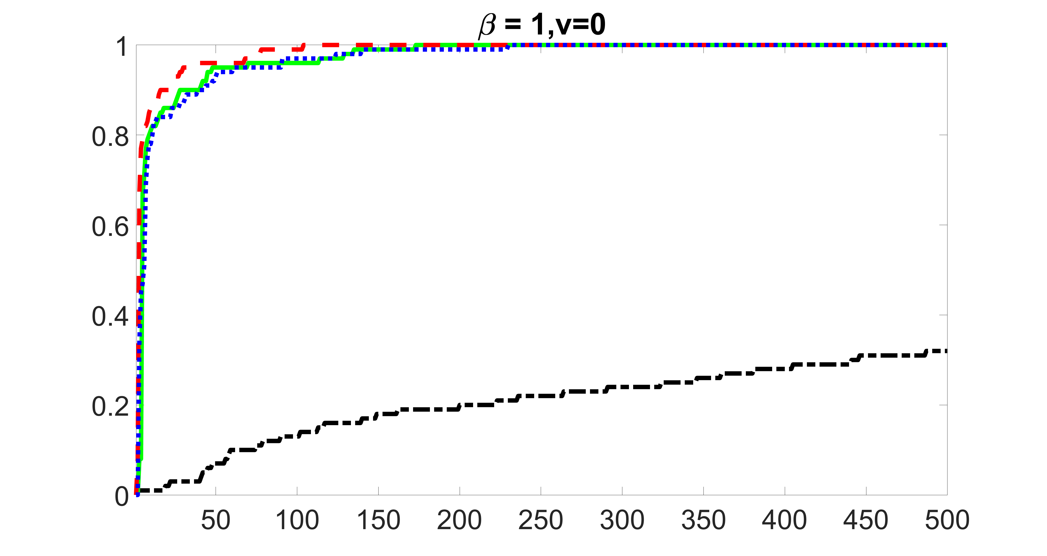
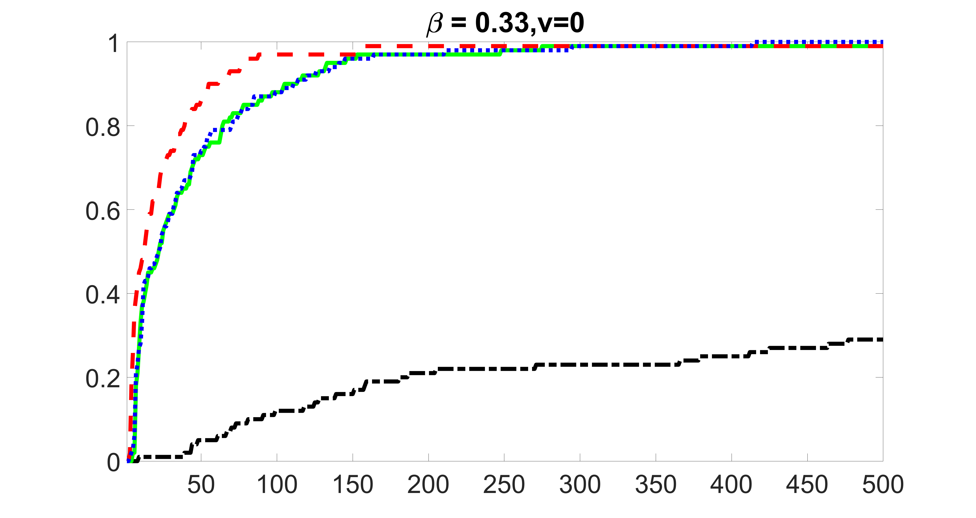
We compare the proposed joint screening procedure to two competing procedures. The first is an outcome screening procedure that selects set For fair comparison, we let range from to . The second is an intersection screening procedure, that selects set . We let range from to , while keeping . Similarly, for those specific sizes that cannot reach, we use linear interpolation to estimate the coverage proportions. We plot the results for in Figure 5. The remaining results for , , , and can be found in Figures 10 – 14 of the supplementary material.
outcome, weak exposure
outcome, medium exposure

outcome, strong exposure
outcome, zero exposure

outcome, zero exposure
outcome, zero exposure
From the plots, one can see that both the “intersection” and “outcome” screening methods miss the confounder with a very high probability even as the size of the selected set approaches . In contrast, our method can select with high probability when is relatively small. For confounders and , all three methods perform similarly. For the precision variables, the “outcome” method and our “joint” method perform similarly in covering these variables, while the “intersection” performs badly. Combining the results, one can see that our method performs the best as our method selects all the confounders and precision variables with high probabilities. In addition, we find that the coverage proportion of our method increases when the sample size increases, which validates the sure independence screening property developed in Section 15 of the supplementary material.
5.2 Simulation for estimation
In this part, we evaluate the performance of our estimation procedure after the first-step screening. For the size of in the screening step, we set . We compare the proposed estimate with the oracle estimate, which is calculated by adjusting for the ideal adjustment set including only confounders and precision variables as and then estimate by using the optimization (3) without imposing the -regularization. We report the mean squared errors (MSEs) for and defined as and , respectively. Table 1 summarizes the average MSEs of the proposed and oracle estimates for and among 100 Monte Carlo runs when , and . We can see that the MSE decreases as the sample size increases. In terms of the primary parameter of interest , the proposed estimate is close to the oracle estimate.
| MSE | MSE | MSE | MSE | ||
|---|---|---|---|---|---|
| n = 200 | |||||
| Proposed | 0.496(0.021) | 0.667(0.005) | Proposed | 0.276(0.009) | 0.528(0.005) |
| Oracle | 0.086(0.005) | 0.624(0.004) | Oracle | 0.021(0.001) | 0.501(0.004) |
| n = 500 | |||||
| Proposed | 0.303(0.008) | 0.574(0.006) | Proposed | 0.191(0.005) | 0.345(0.004) |
| Oracle | 0.036(0.002) | 0.553(0.005) | Oracle | 0.006(0.000) | 0.340(0.004) |
| n = 1000 | |||||
| Proposed | 0.217(0.004) | 0.449(0.004) | Proposed | 0.128(0.006) | 0.234(0.002) |
| Oracle | 0.013(0.001) | 0.460(0.005) | Oracle | 0.003(0.000) | 0.233(0.002) |
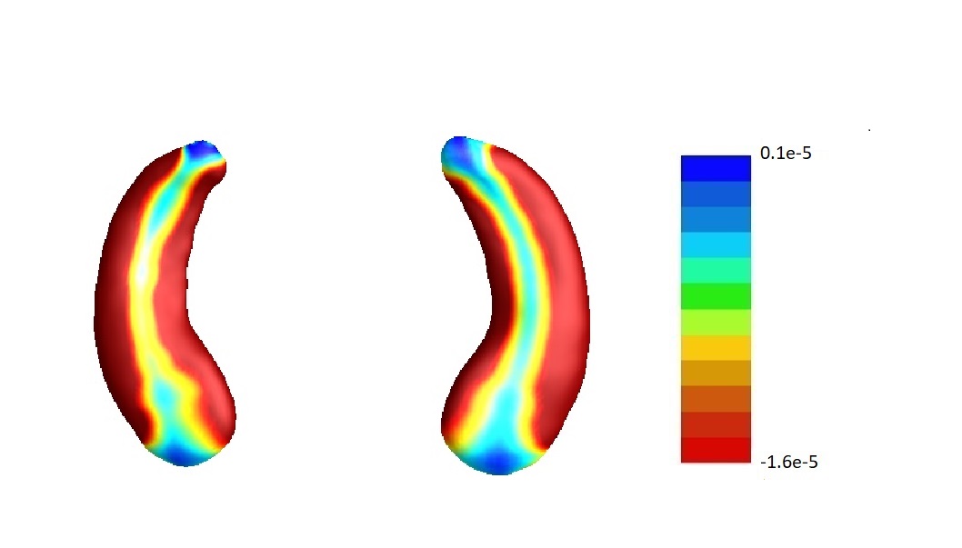
We plot the 2D map of based on the average of 100 Monte Carlo runs in Figure 6(c). For comparison, we also plot the corresponding average oracle estimate in Figure 6(b) and the true in Figure 6(a). One can see that the proposed method recovers the signal pattern reasonably well.
We also report the sensitivity and specificity of the estimates in Section 14.1 of the supplementary material. We have found that although the proposed method may not remove all of the instrumental variables, eliminating even just some of the instruments greatly reduces the MSEs of both and , compared to the method where we do not impose -regularization on in the second-step estimation.
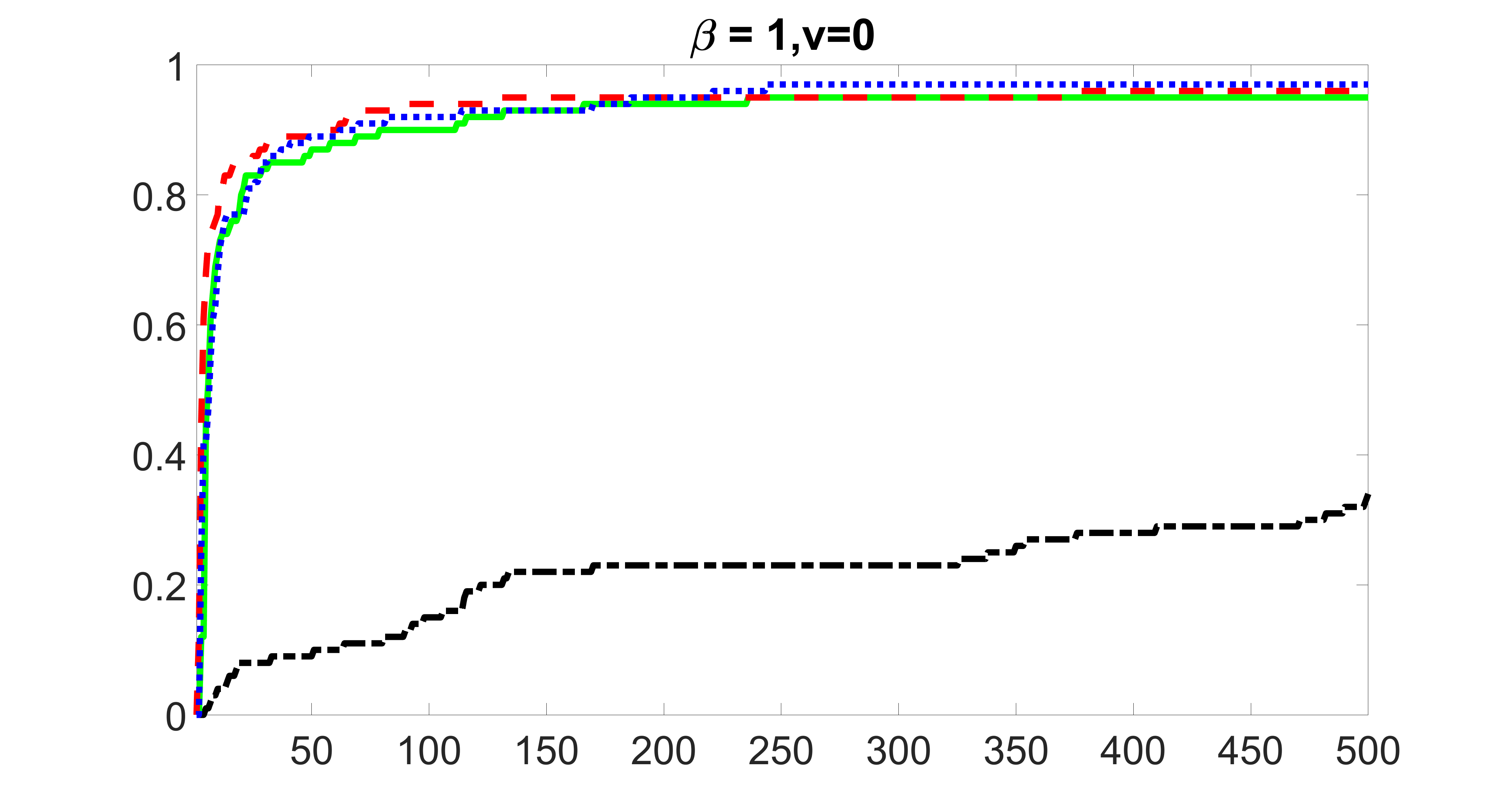
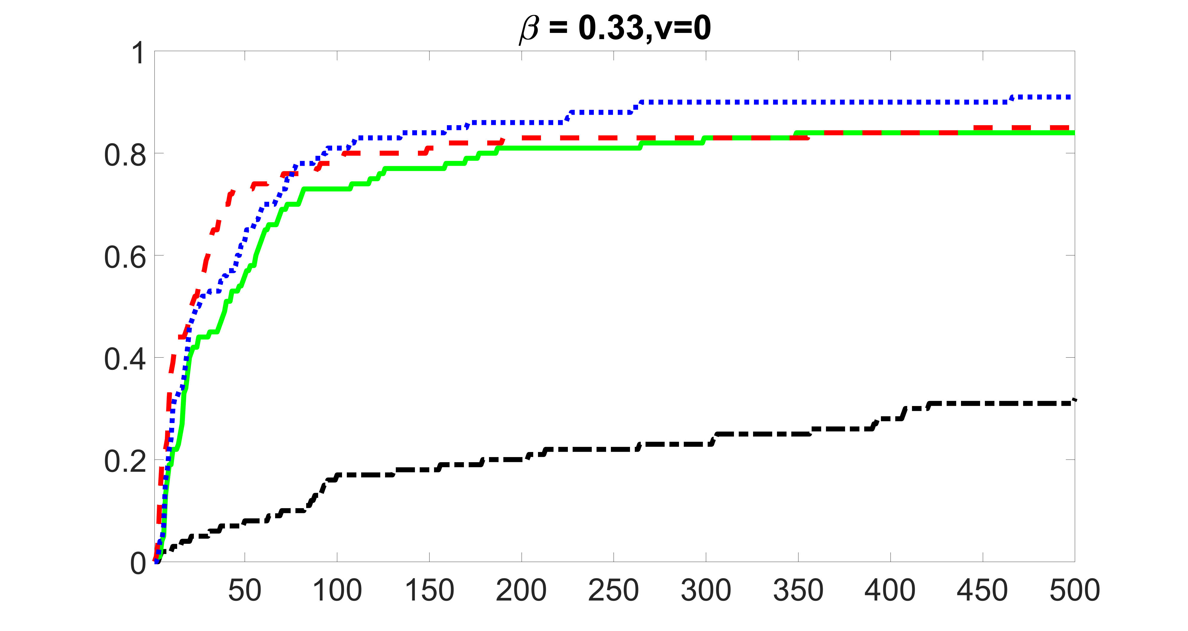
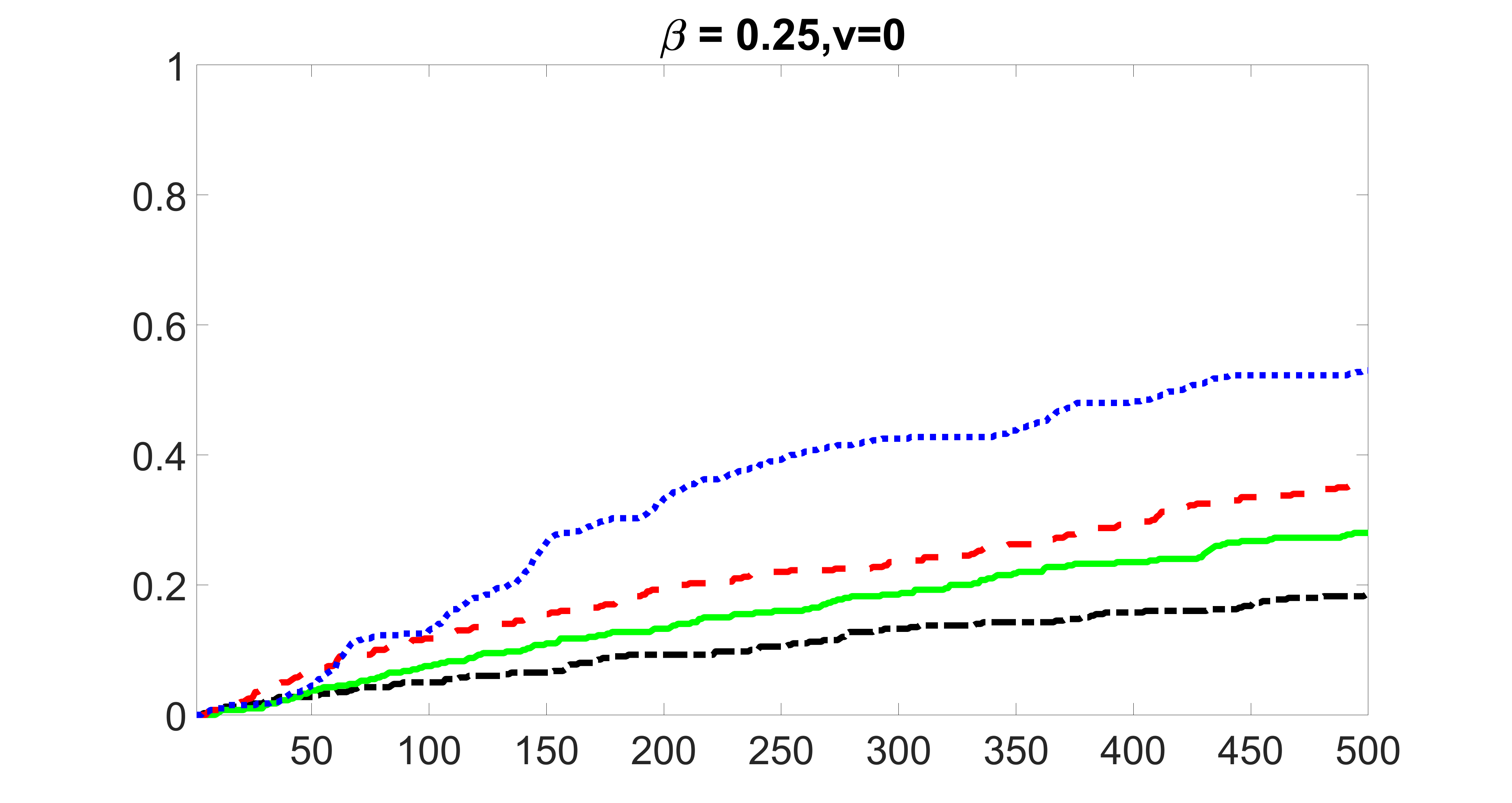
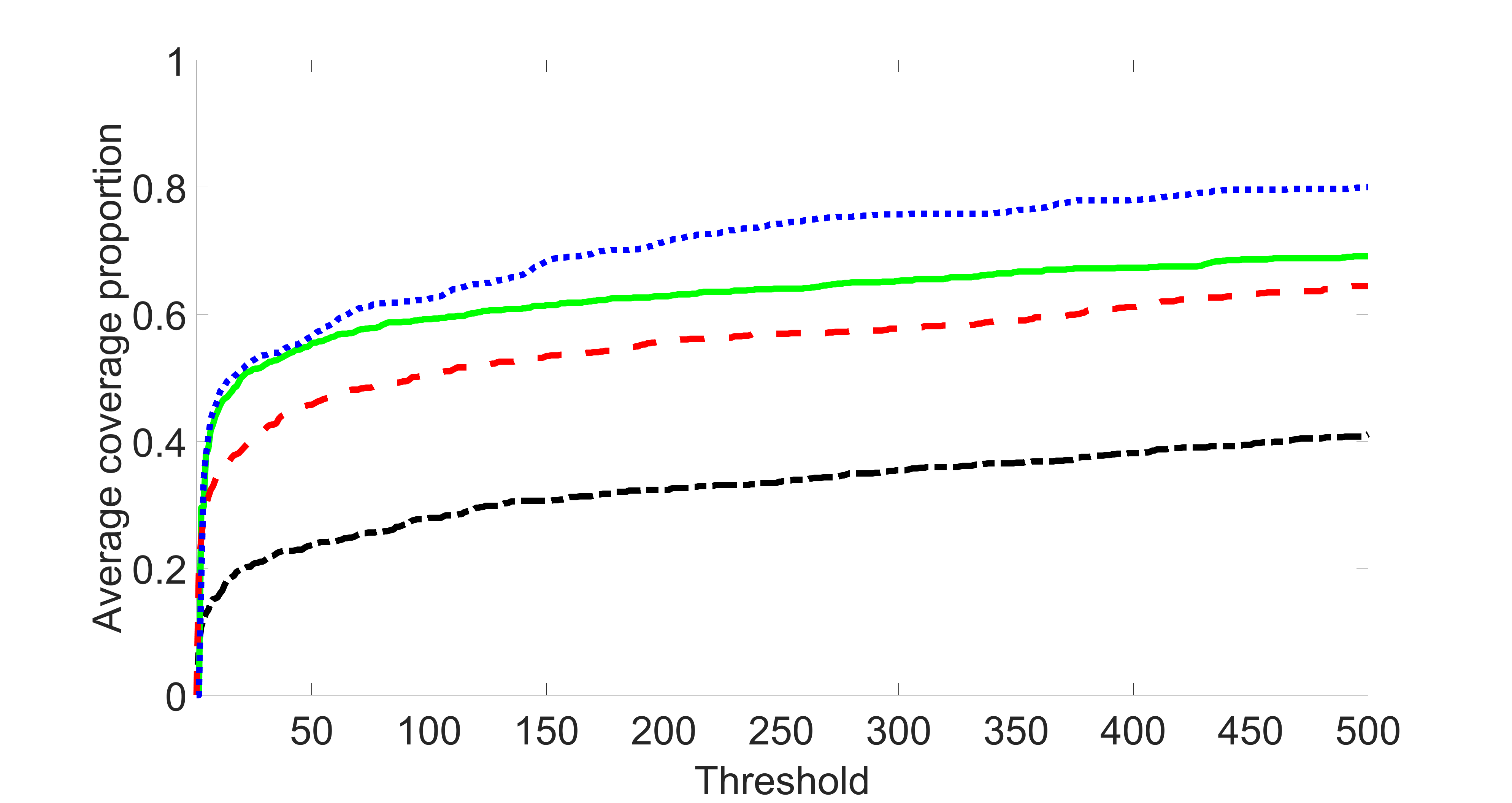
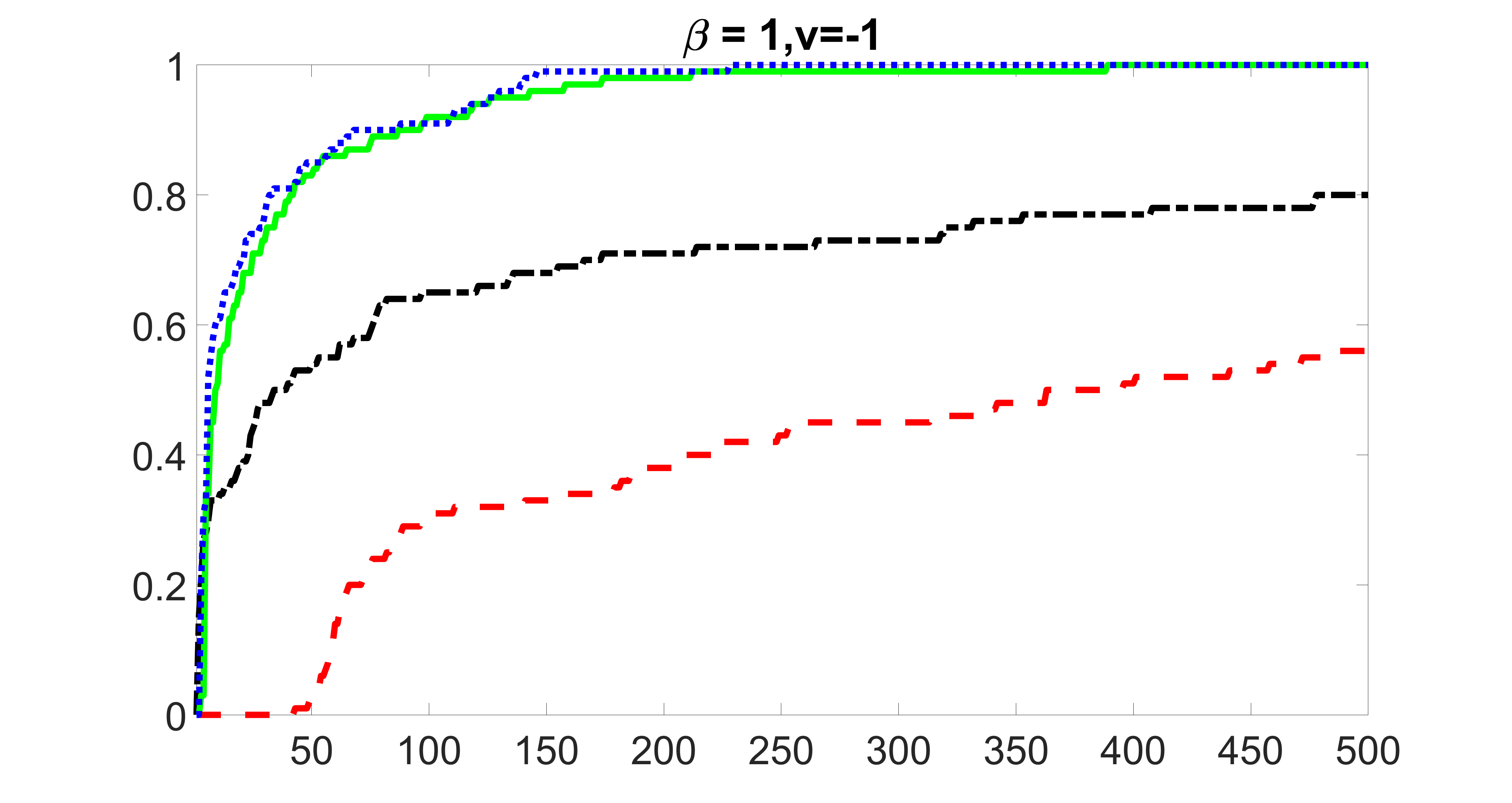
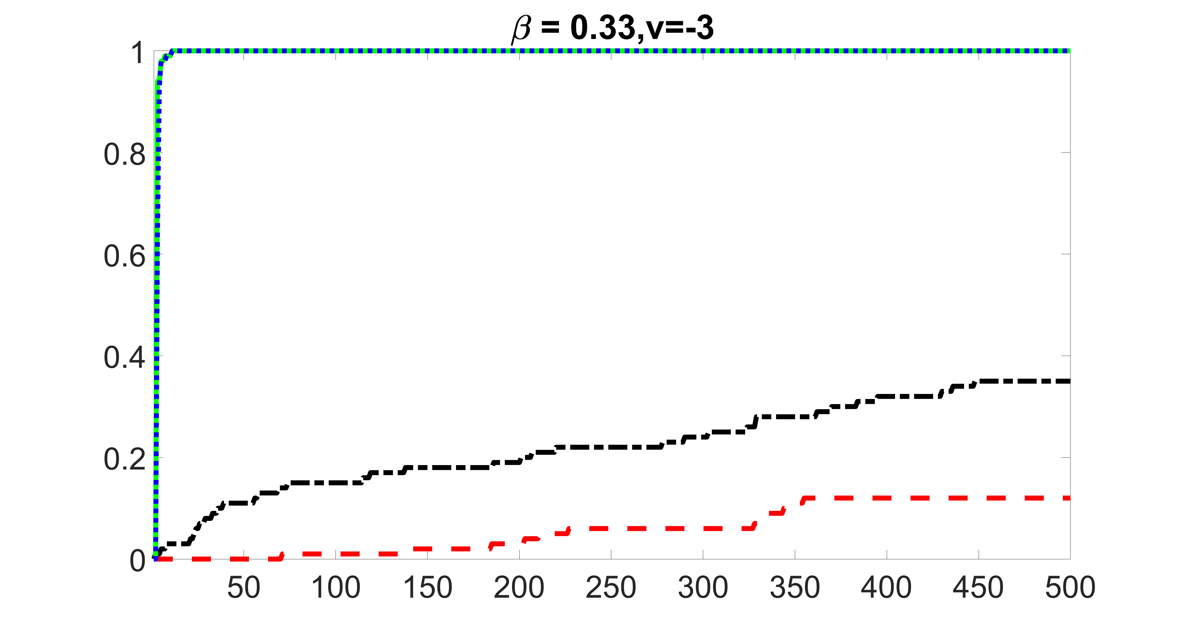
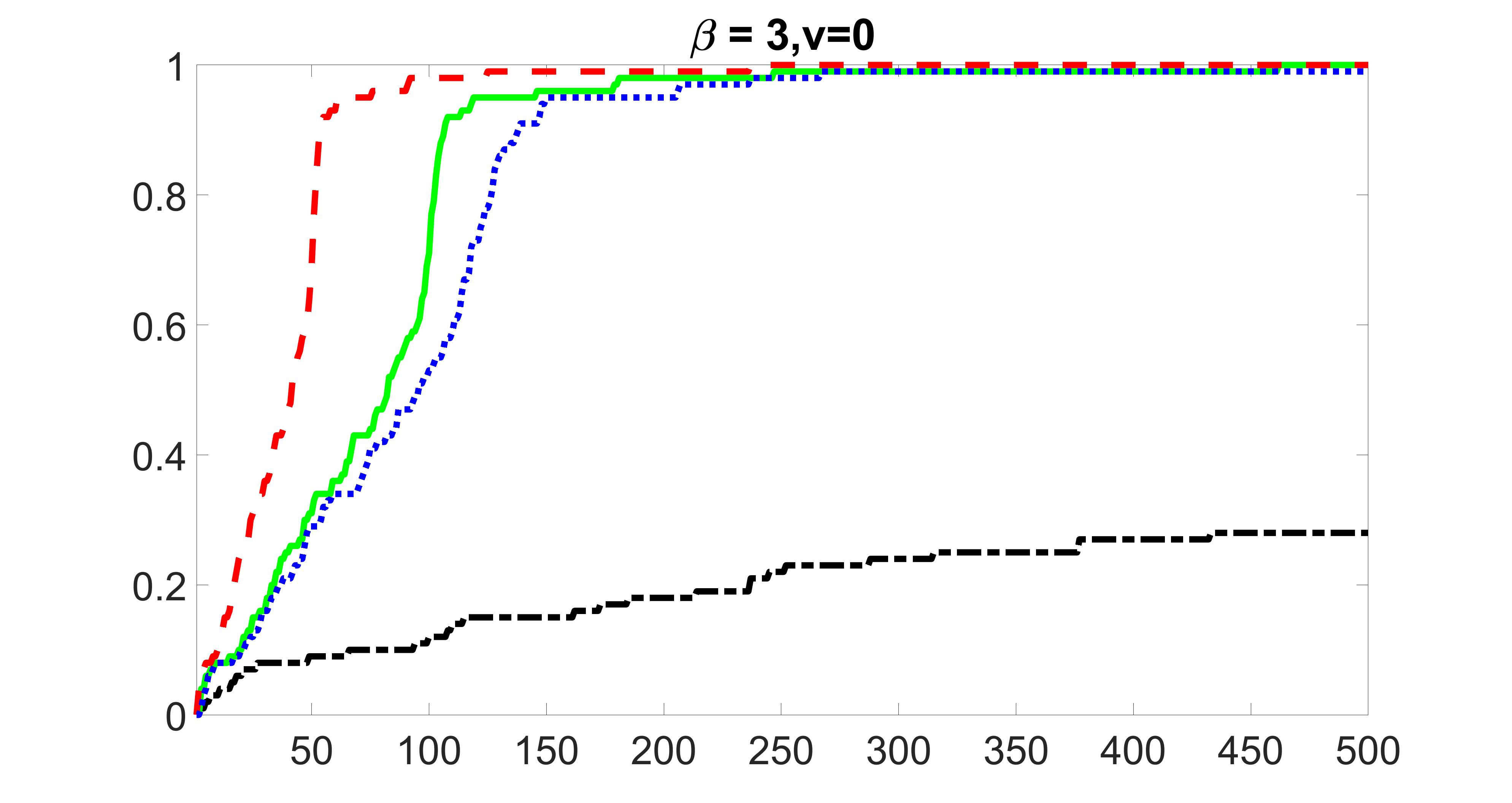
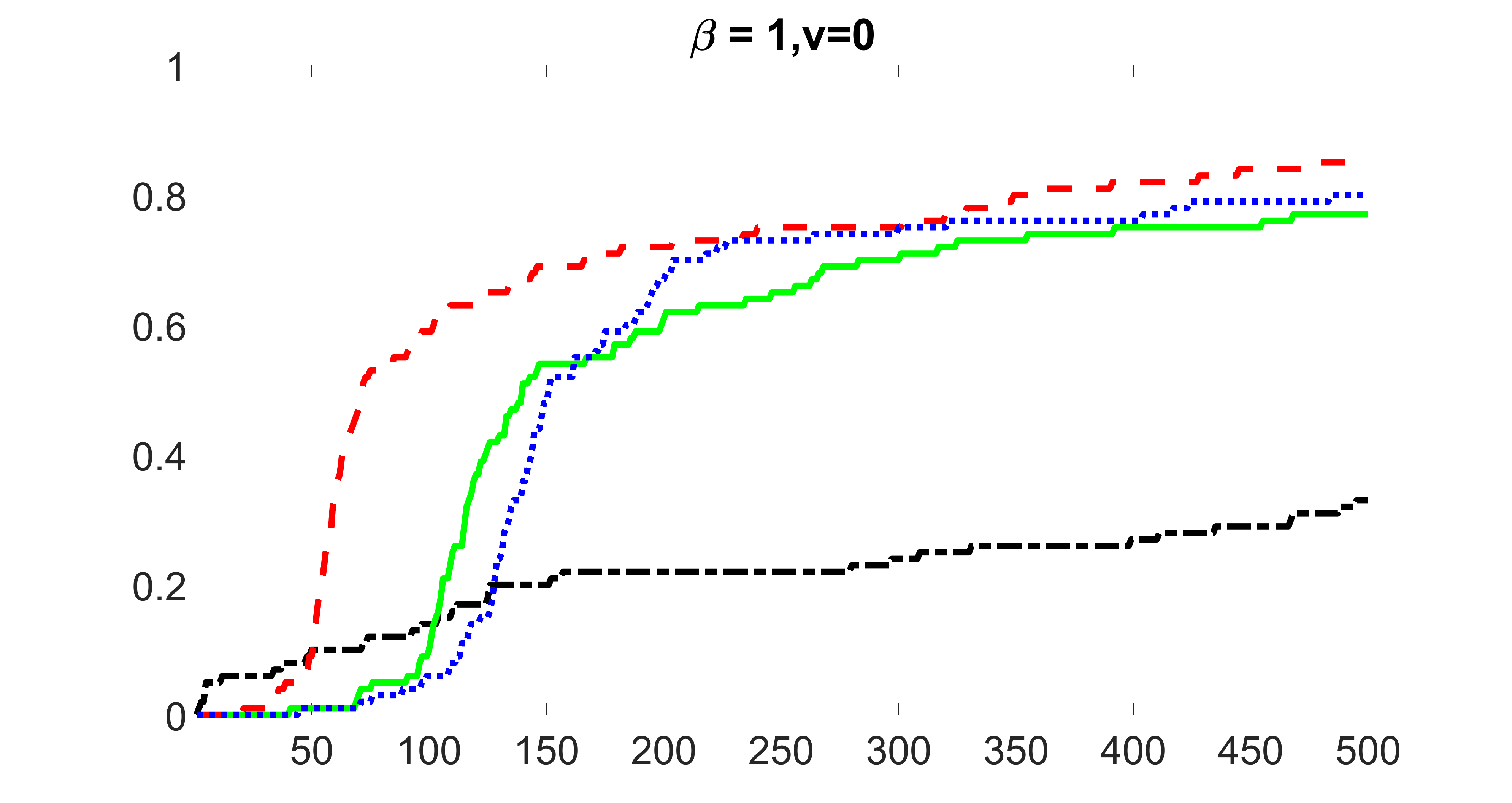
5.3 Screening and estimation using blockwise joint screening
Linkage disequilibrium (LD) is a ubiquitous biological phenomenon where genetic variants present a strong blockwise correlation (LD) structure (Wall and Pritchard, 2003). In Section 3.4, we propose the blockwise joint screening procedure to appropriately utilize LD blocks’ structural information. The performance of this procedure is illustrated in this section using an adapted simulation based on the settings of Dehman et al. (2015).
For , is independently generated from an -dimensional multivariate distribution , where is block-diagonal. If are in the same block, the covariance , else , and the diagonal elements s are all set to . We set to , or according to whether , , or , where and are thresholds determined for producing a given minor allel frequency (MAF). For instance, choosing and , where is the c.d.f. of standard normal distribution, corresponds to a given fixed MAF. In order to generate more realistic MAF distributions, we simulate genotype , where the MAF for each is uniformly sampled between 0.05 and 0.5 (Dehman et al., 2015).
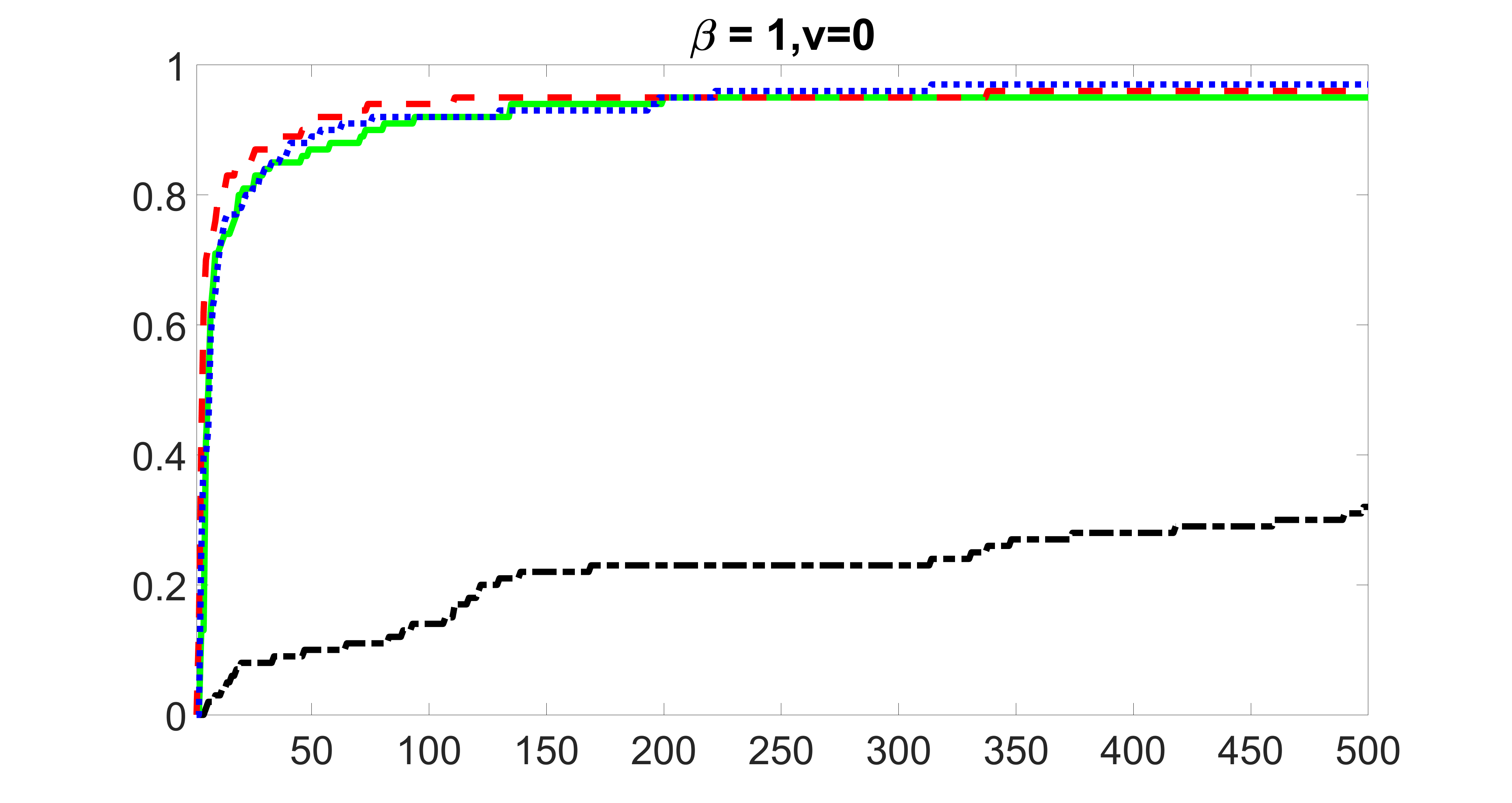
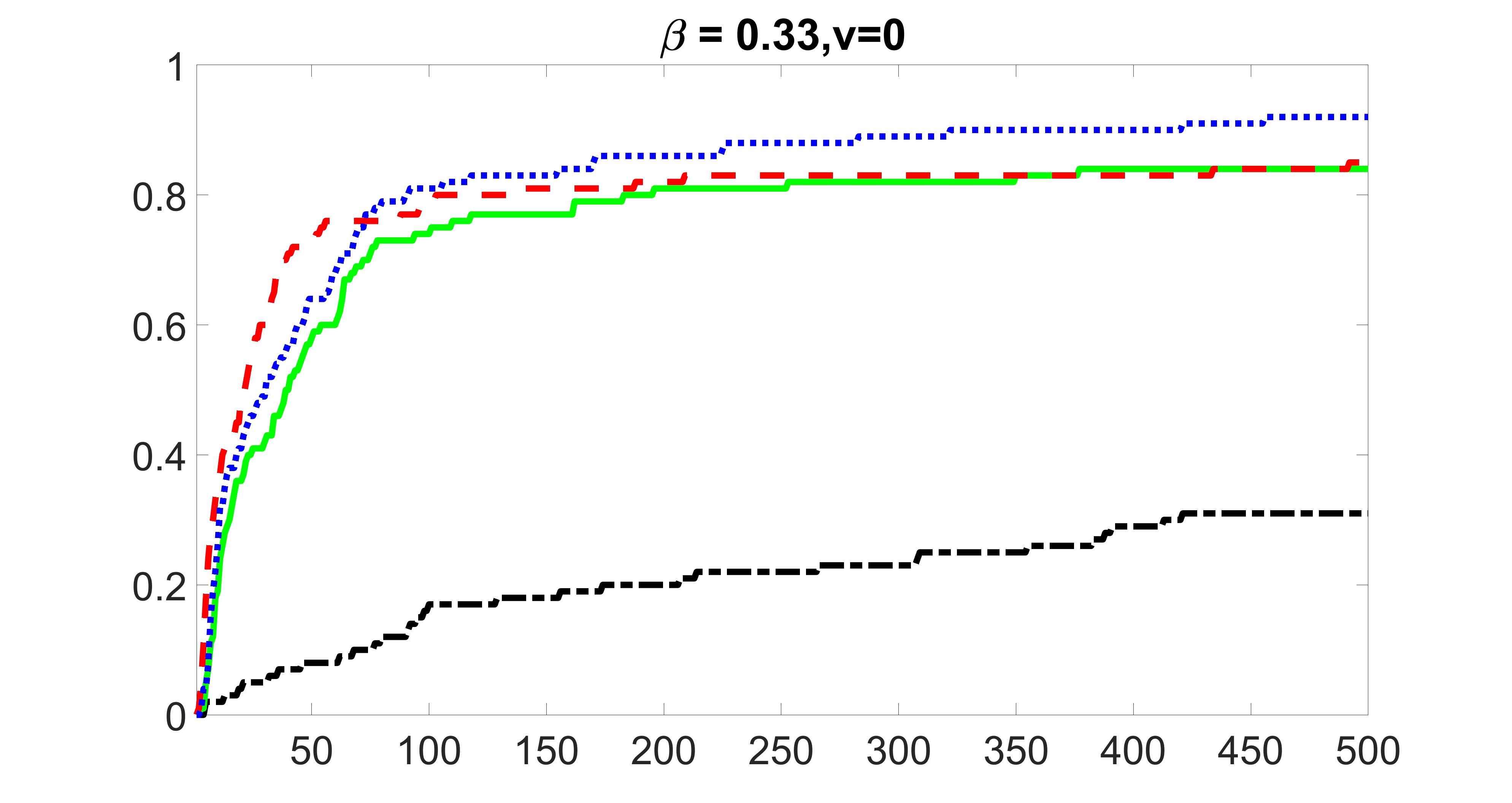
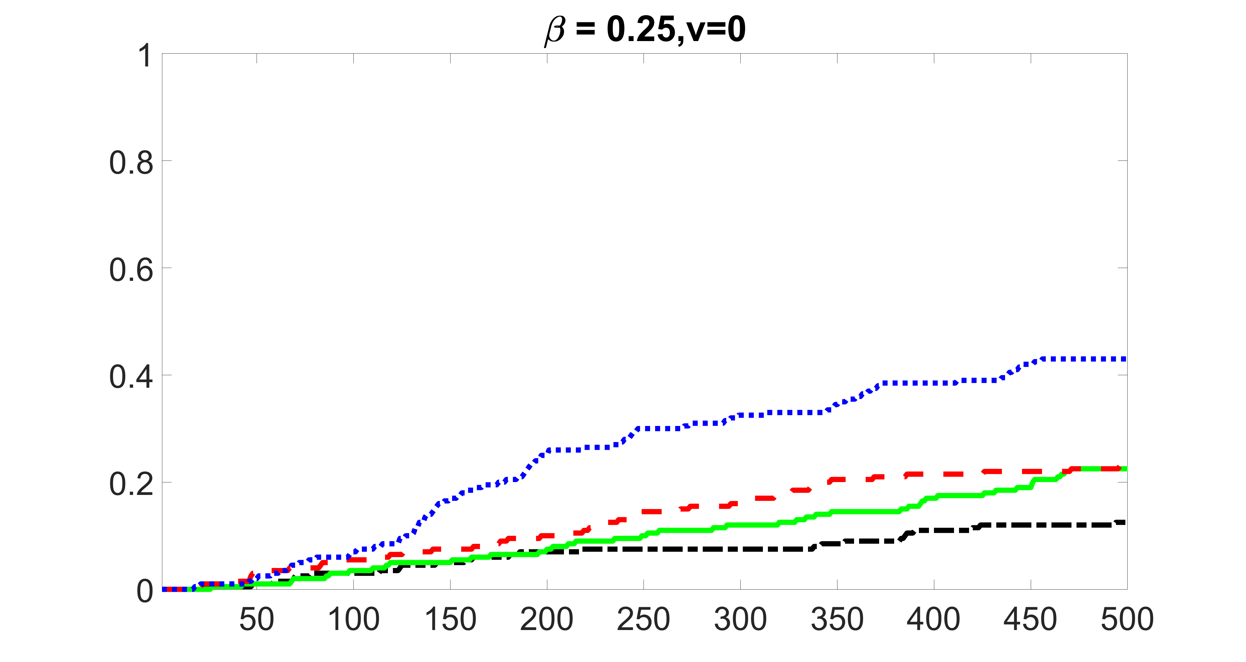
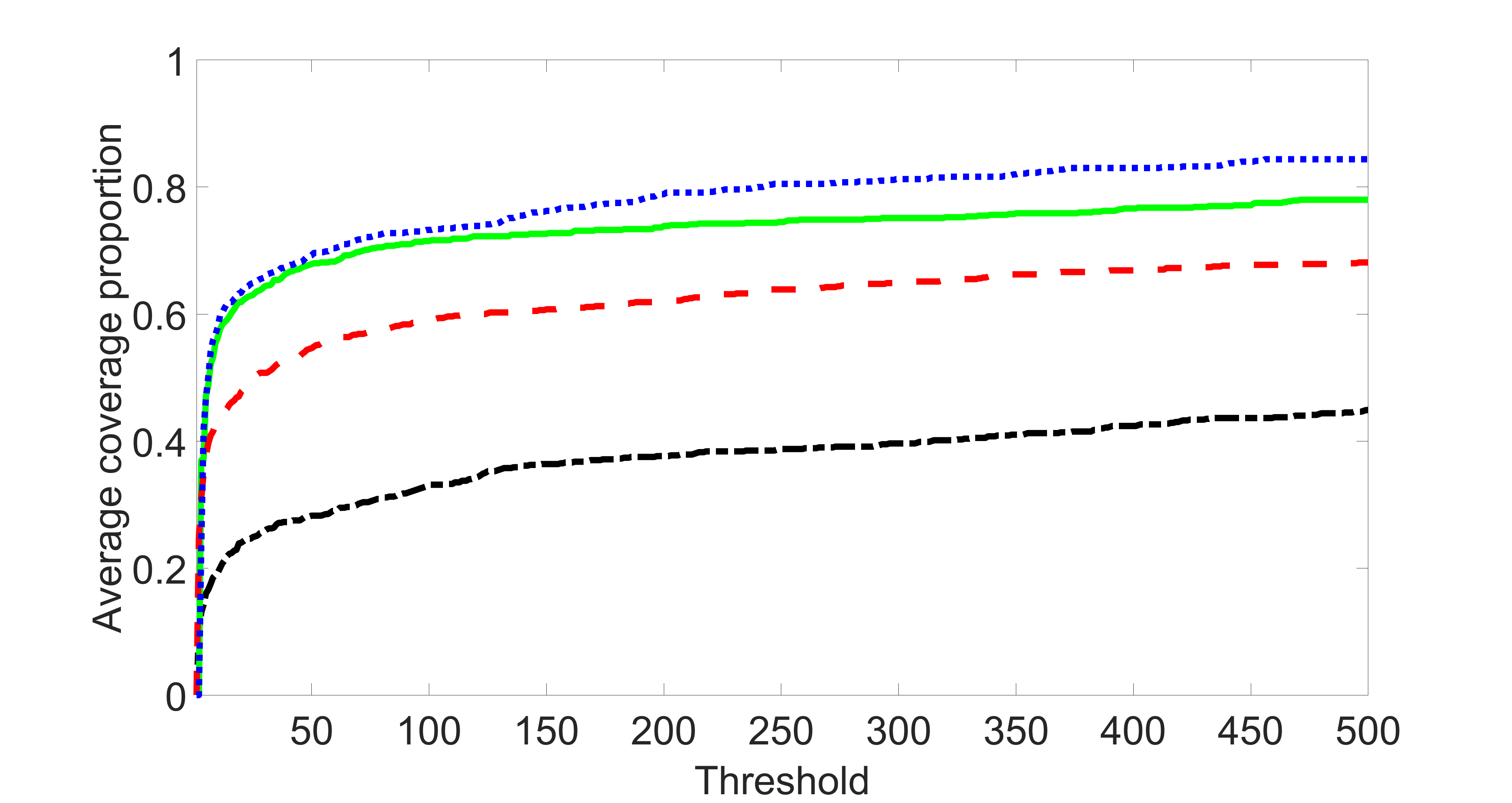
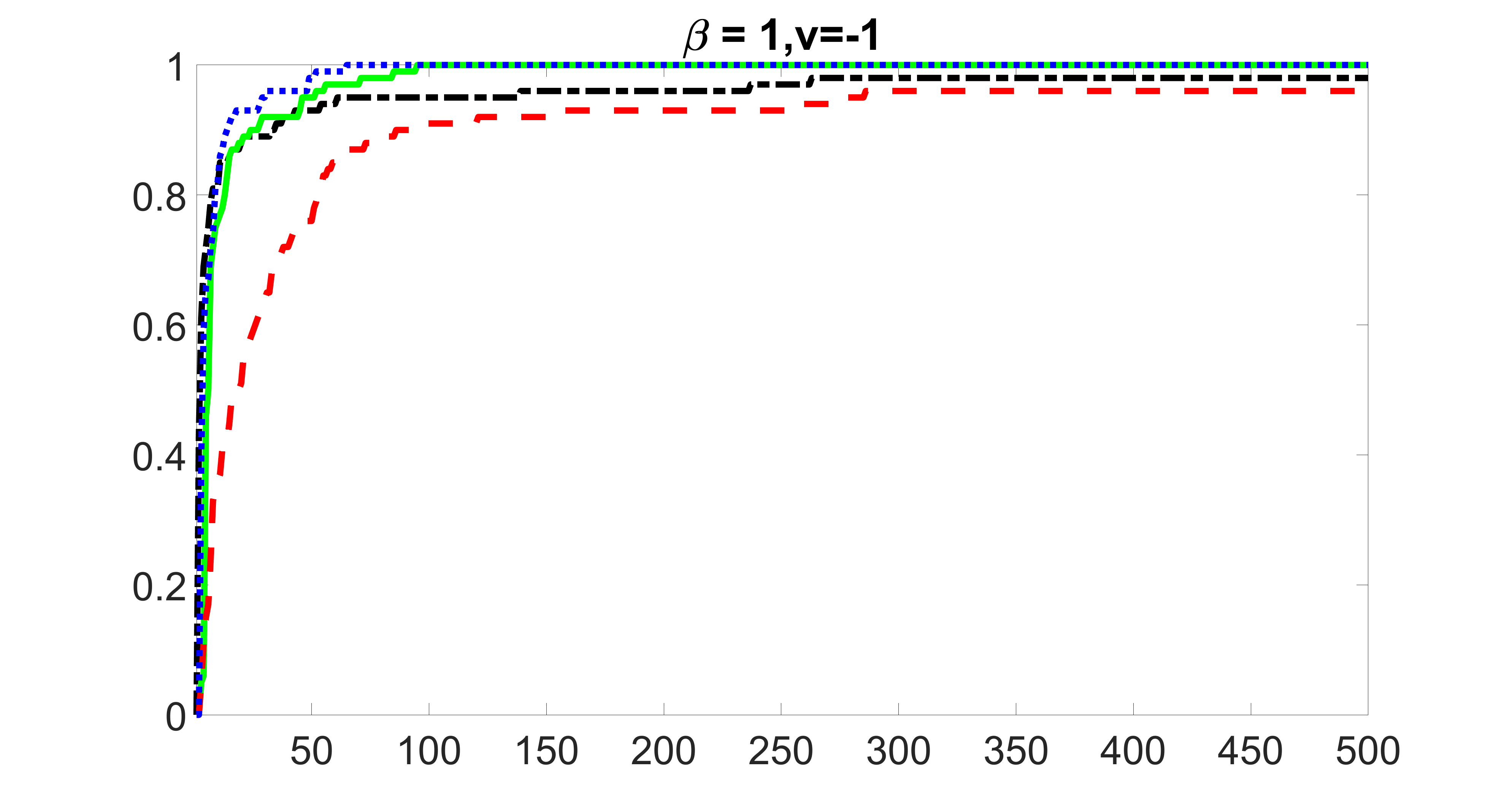
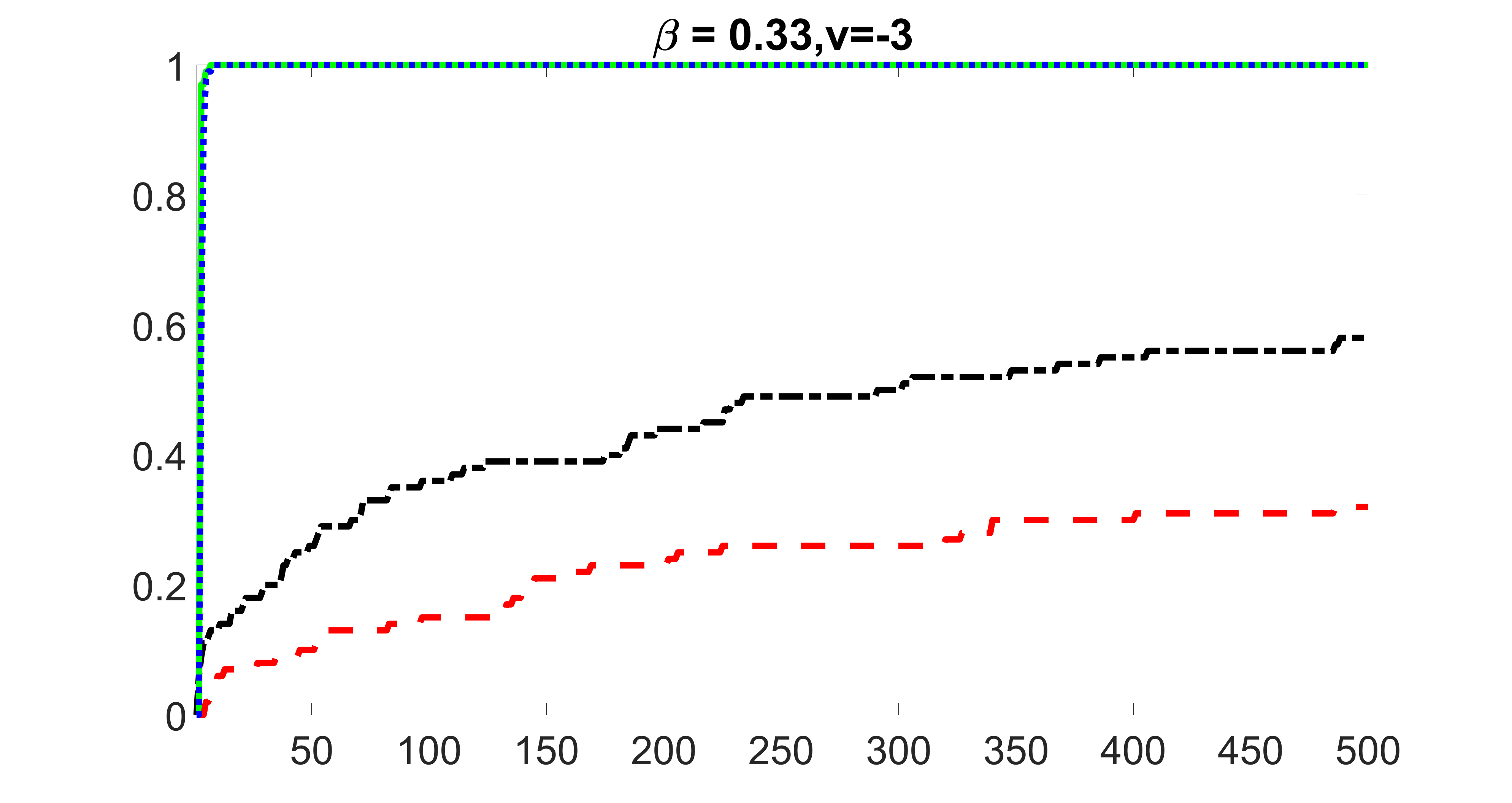
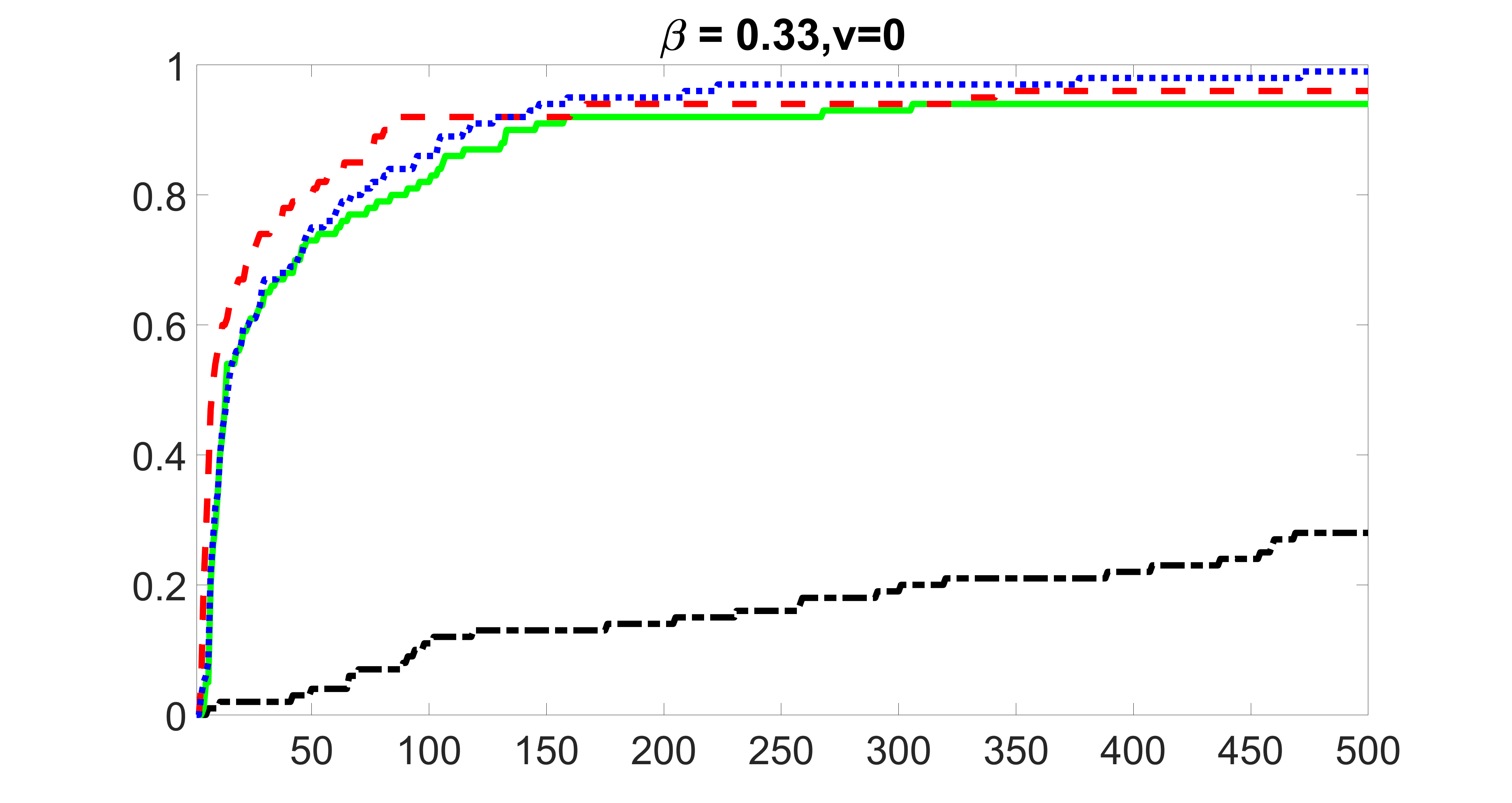
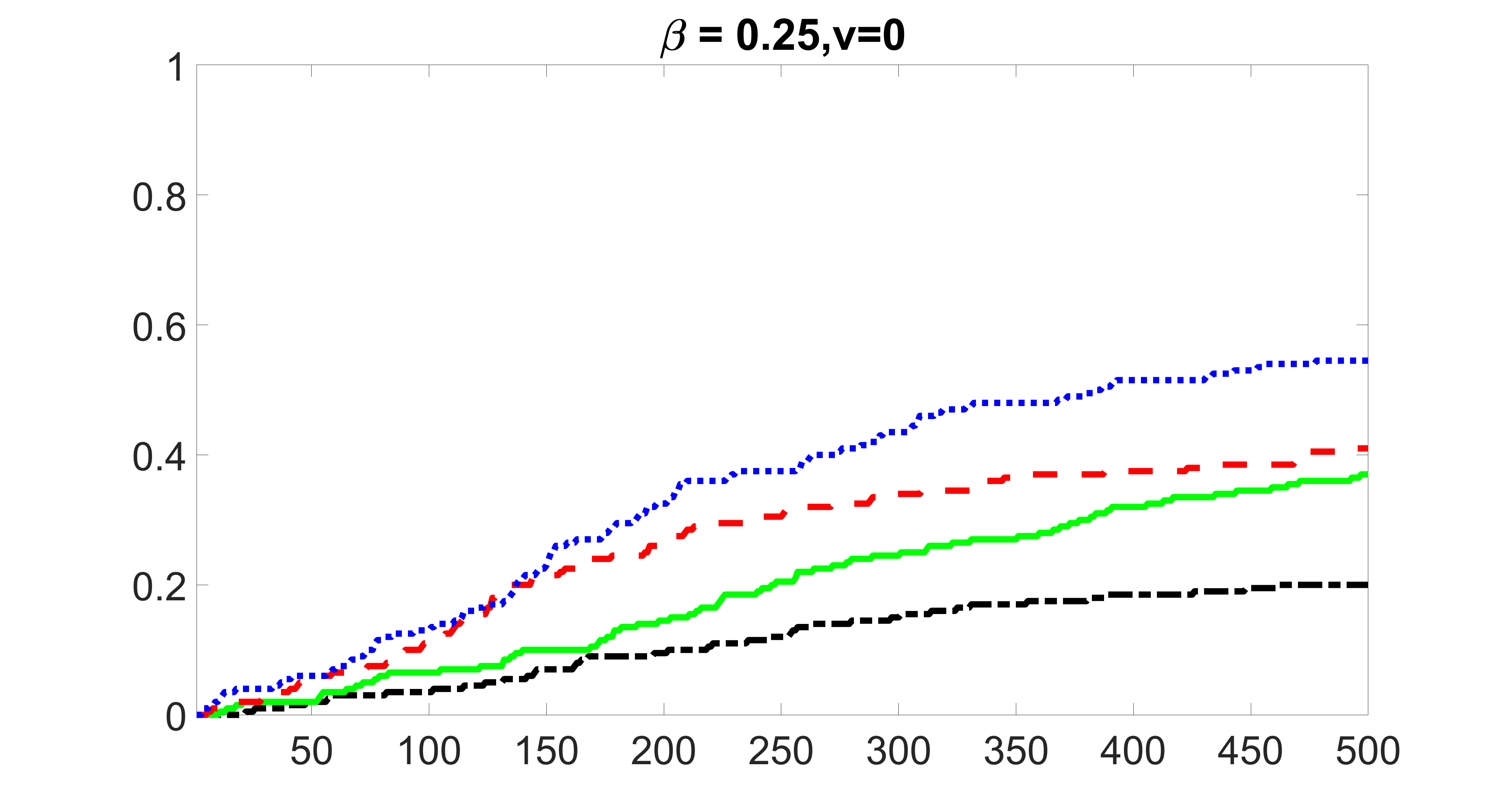
Adapting the simulation setting of Section 5.1 according to Dehman et al. (2015), we set , with blocks of covariates of size replicated times. We perform 100 Monte Carlo runs, and the ordering of the block is drawn at random for each run. The settings for and remain the same as before: is as in Figure 5(a), and is as in Figure 5(b). Further we set , where , , , , , , and for and . We set , , , , , , = for , and otherwise. Here is a randomly selected block consisting of consecutive indices from , where . We have , , and . The other settings are the same as the ones in Section 5.1.
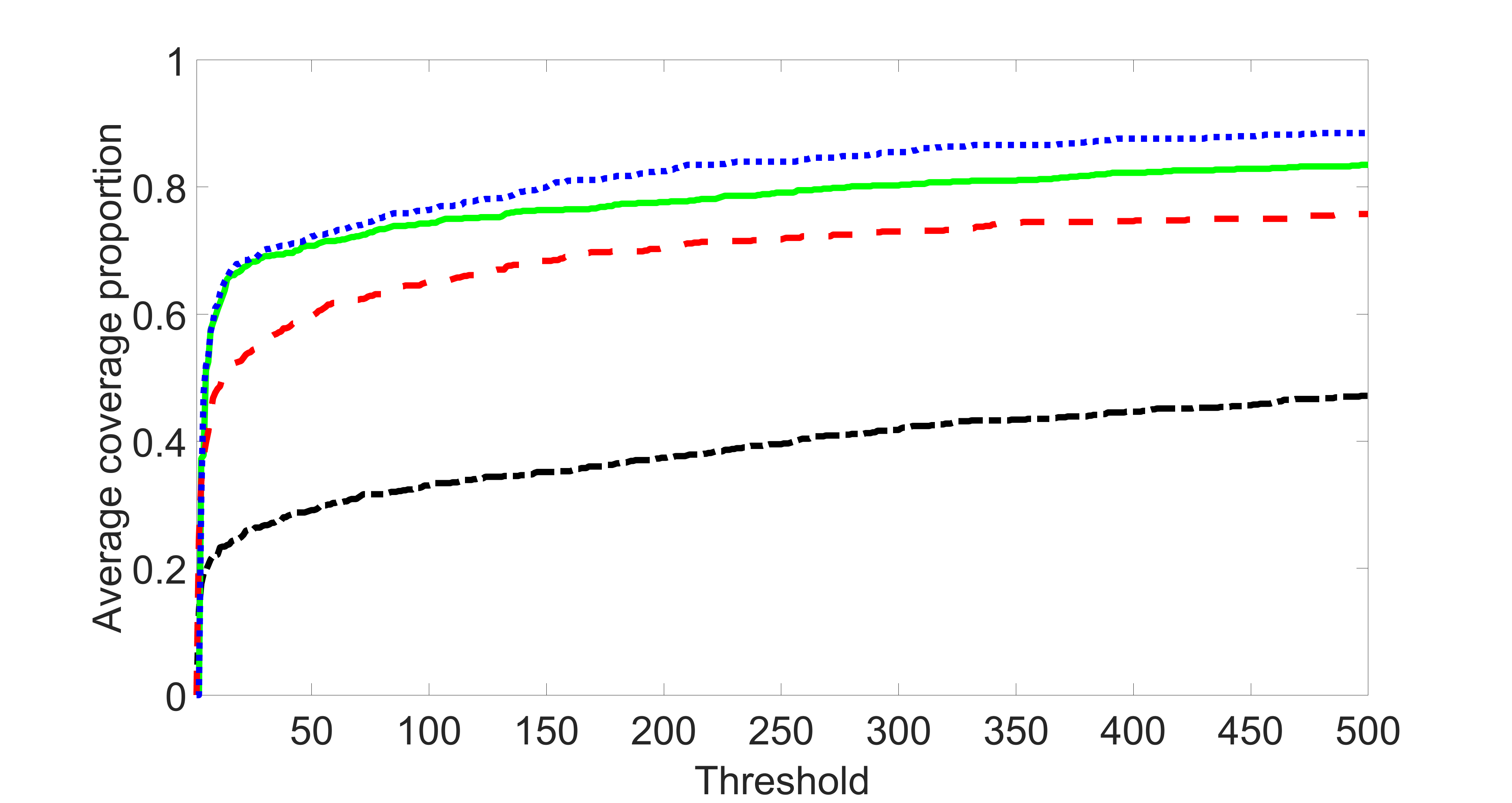
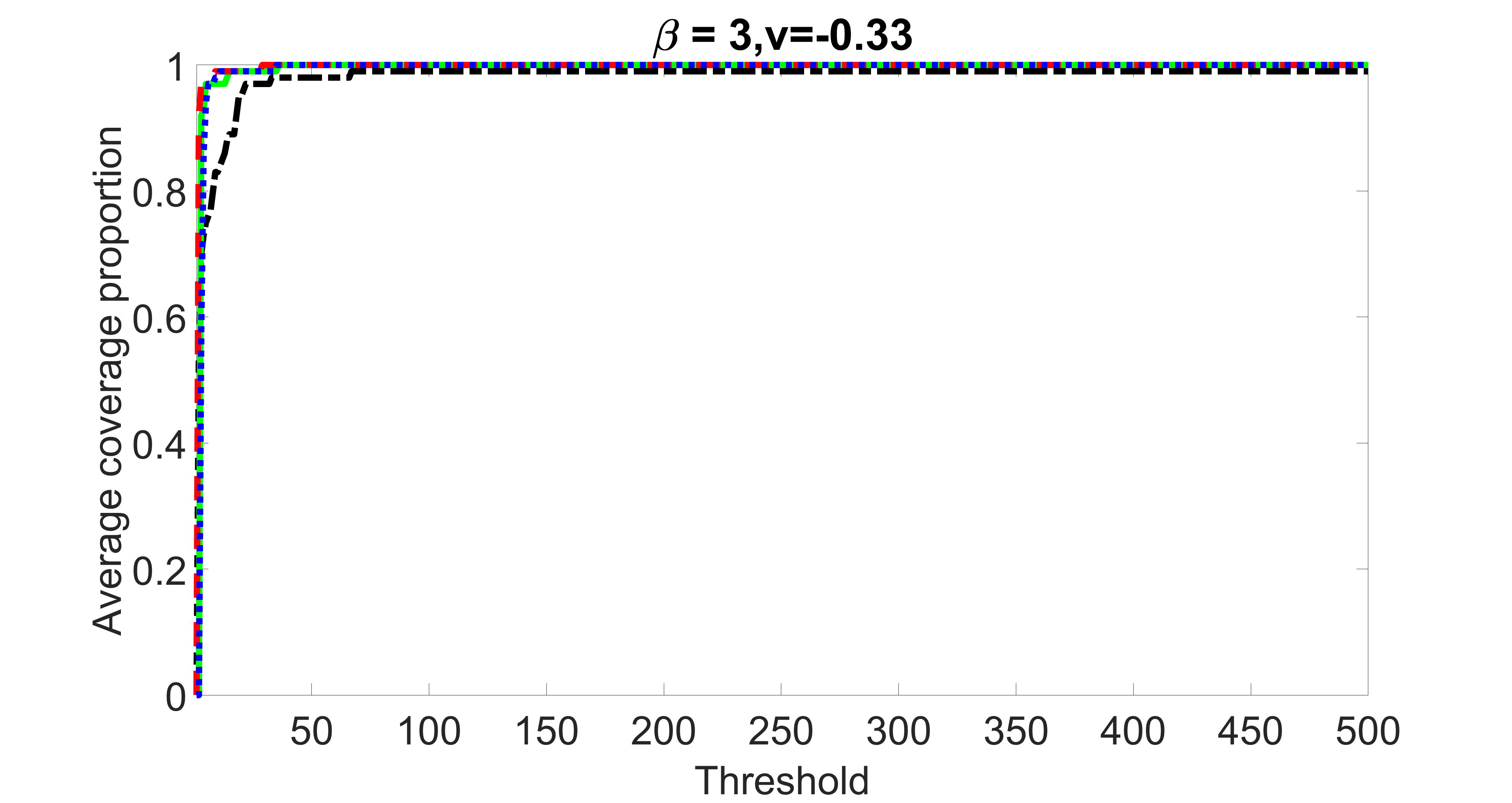
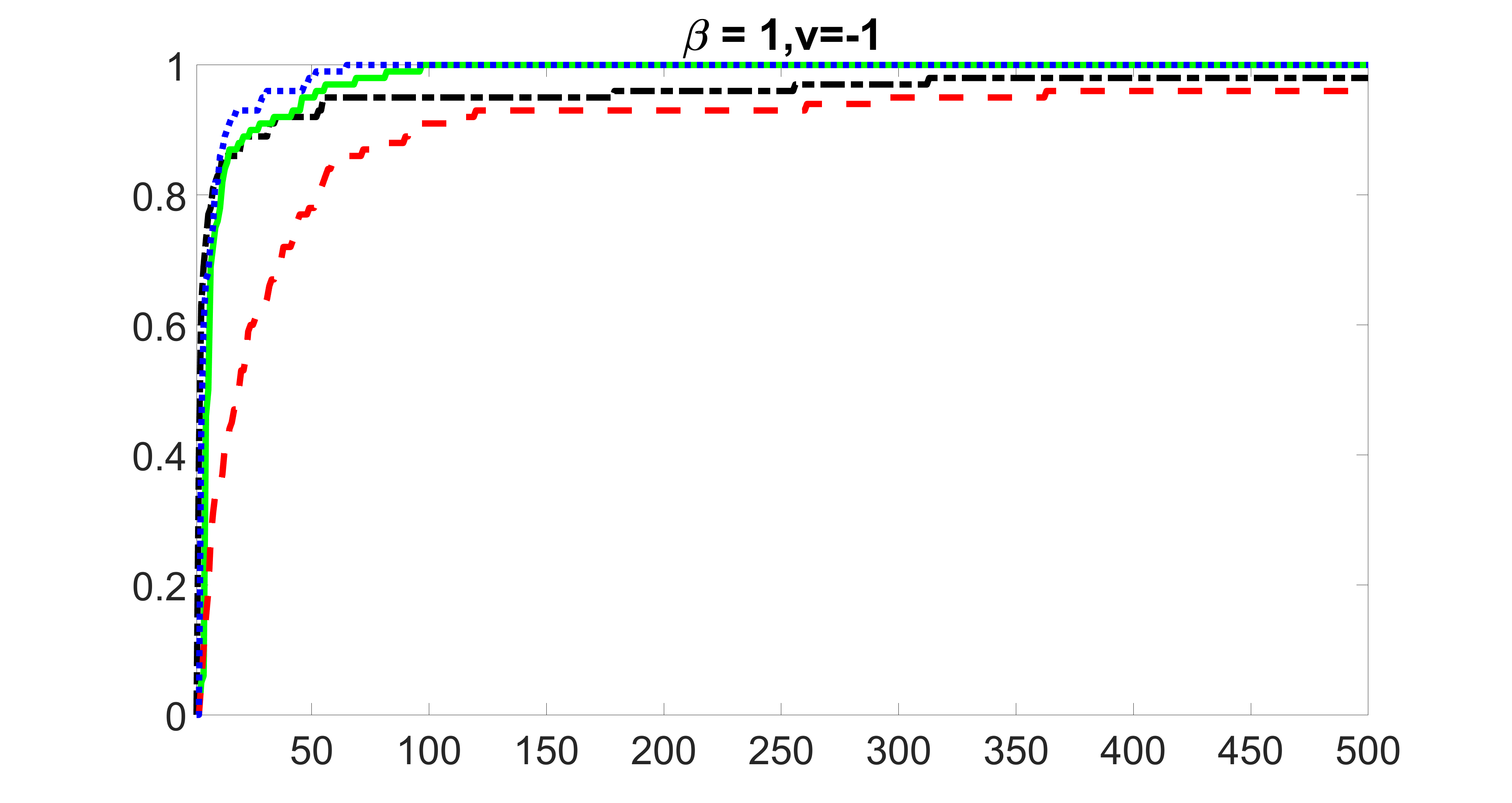
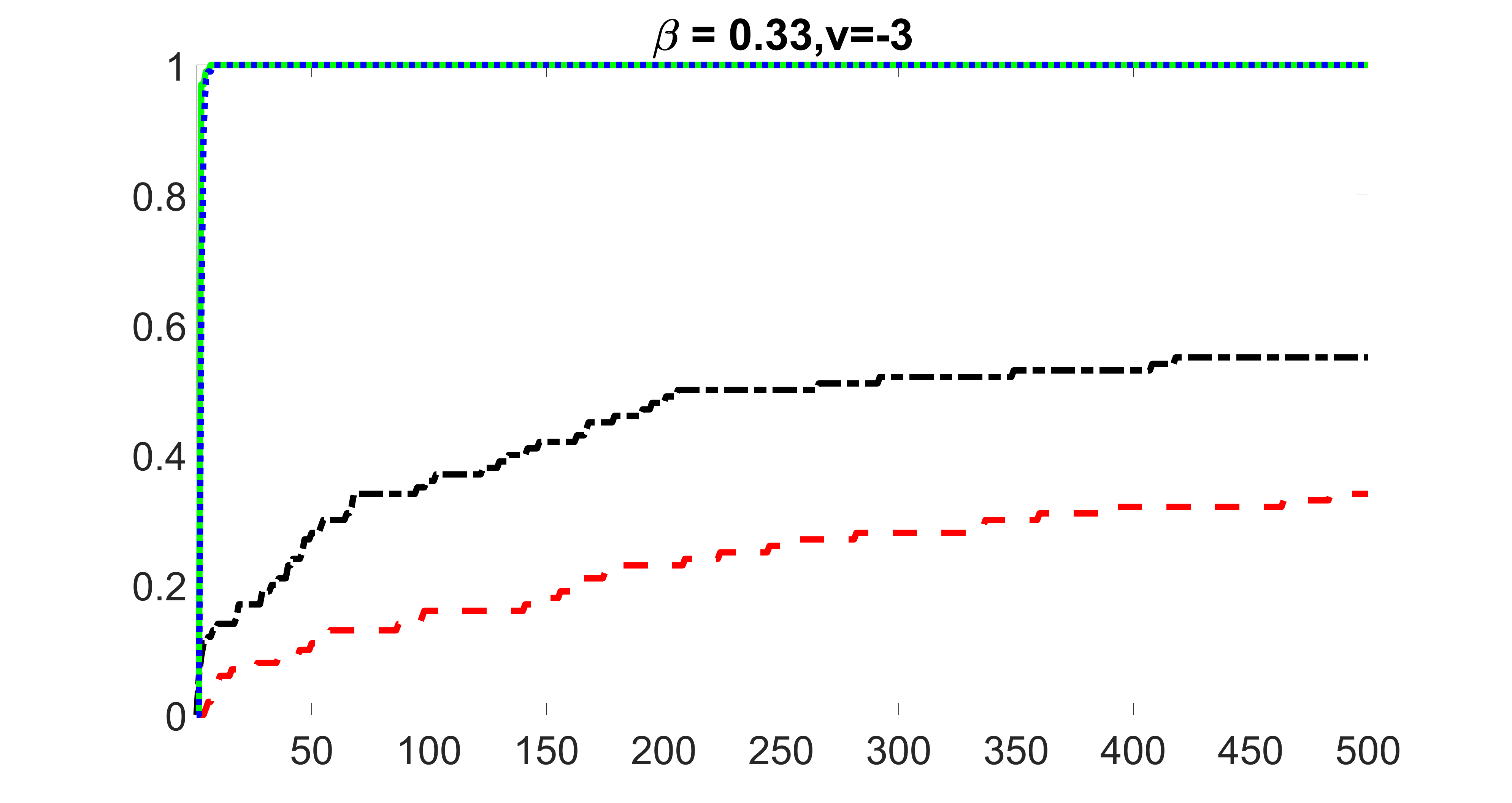
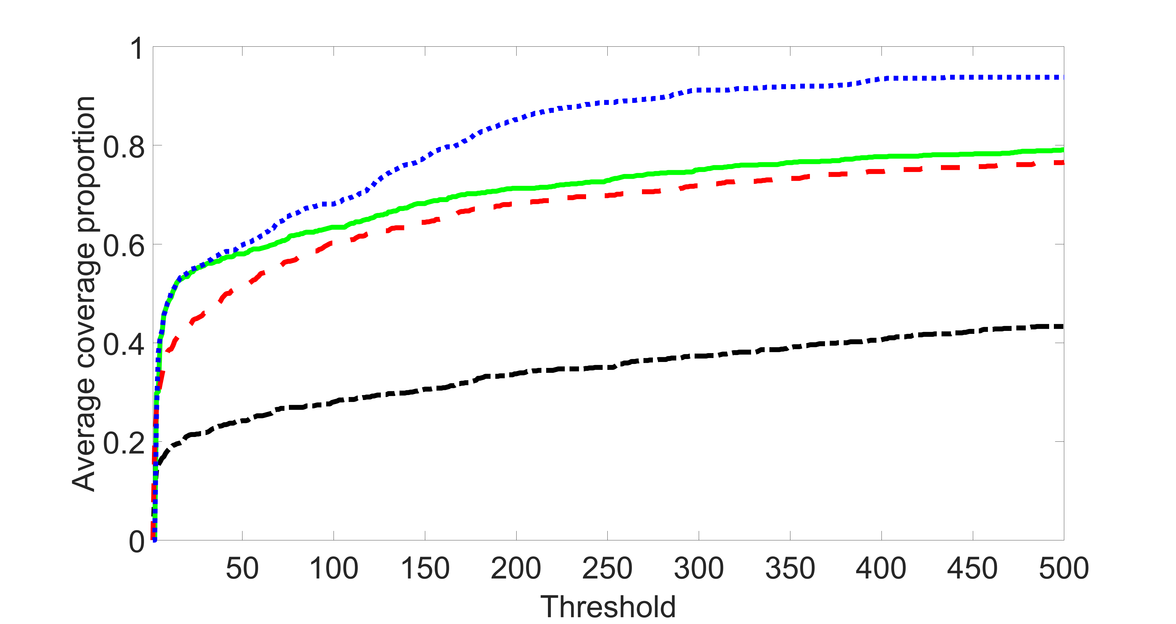
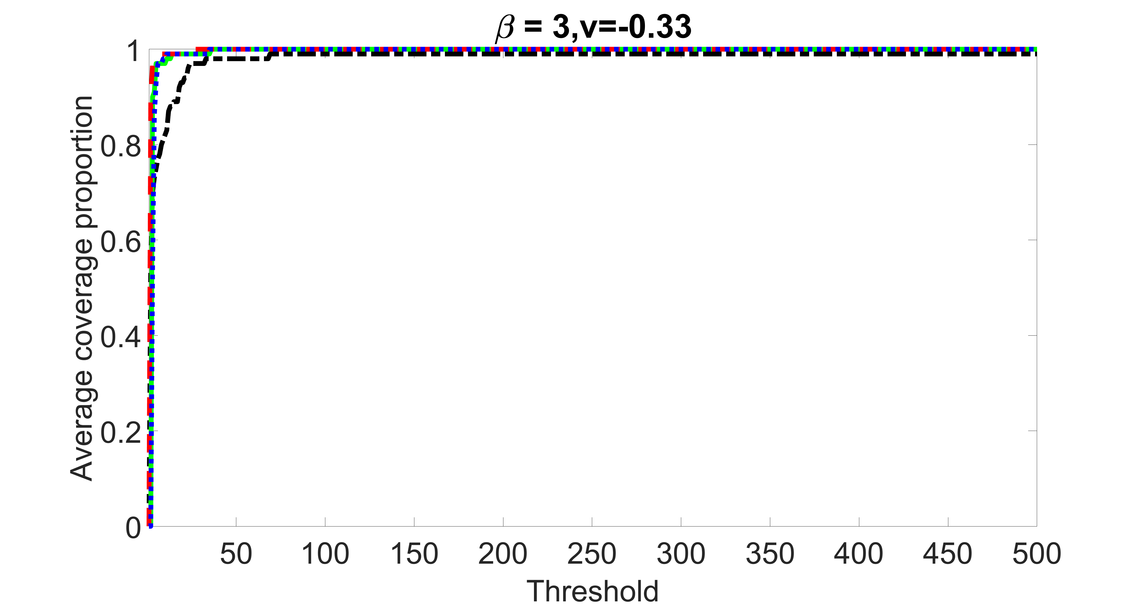
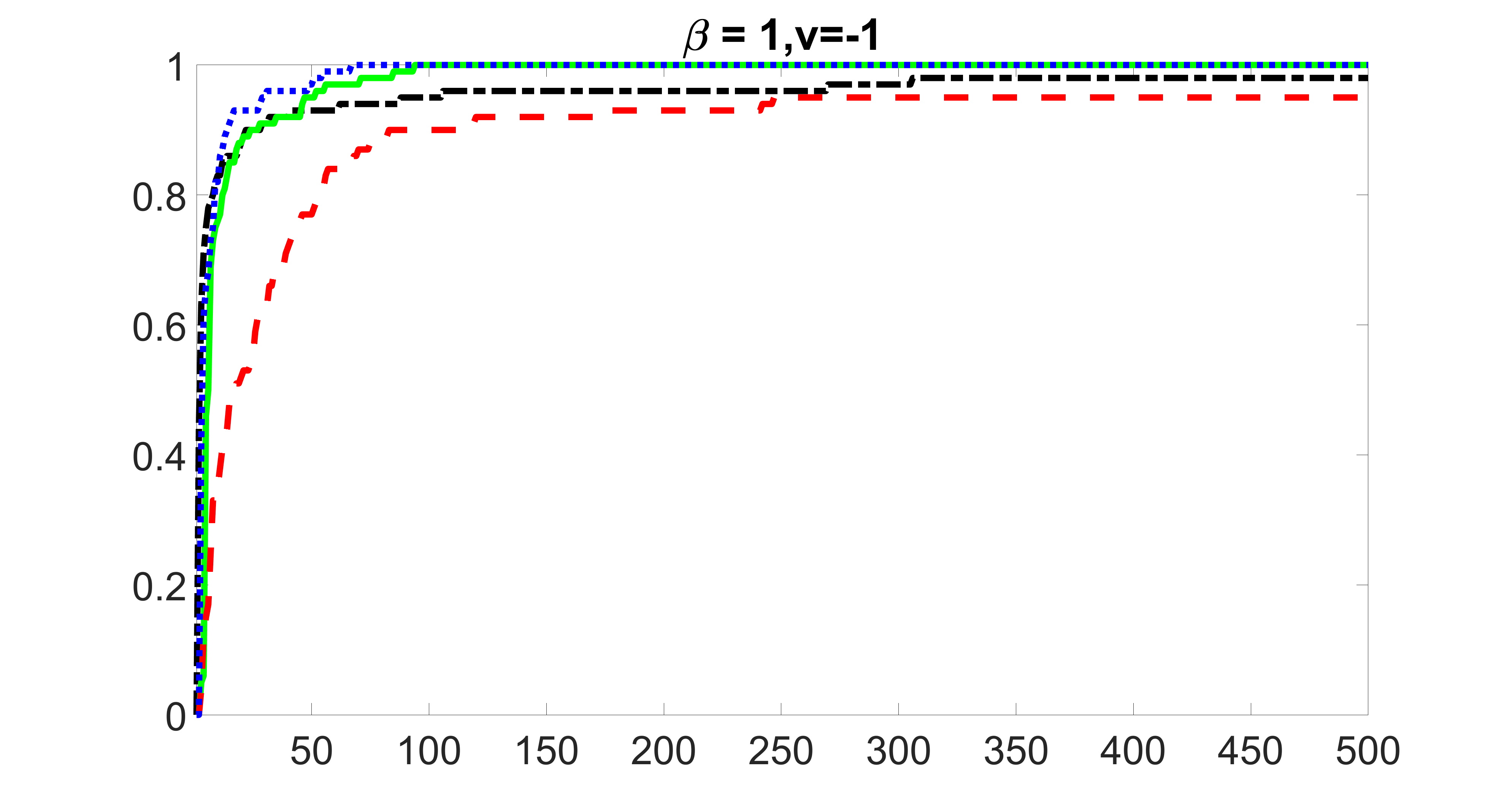
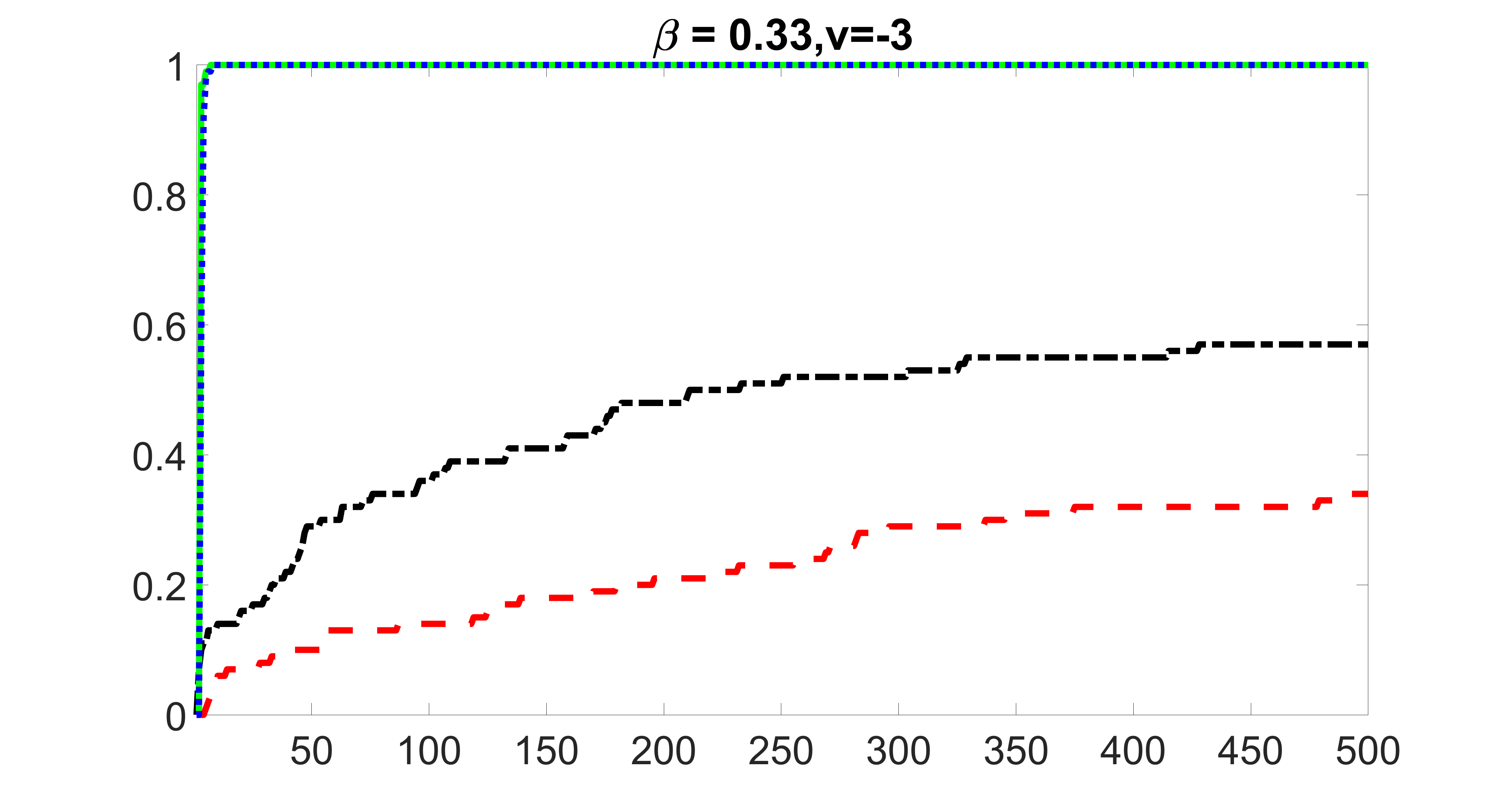
We consider three different sample sizes , and . We first perform the screening procedure and report the coverage proportion of . We also report the coverage proportion for each of the confounding and precision variables. In particular, we include the screening results, in which , , , and , can be found in Figures 29 – 46 of the supplementary material.
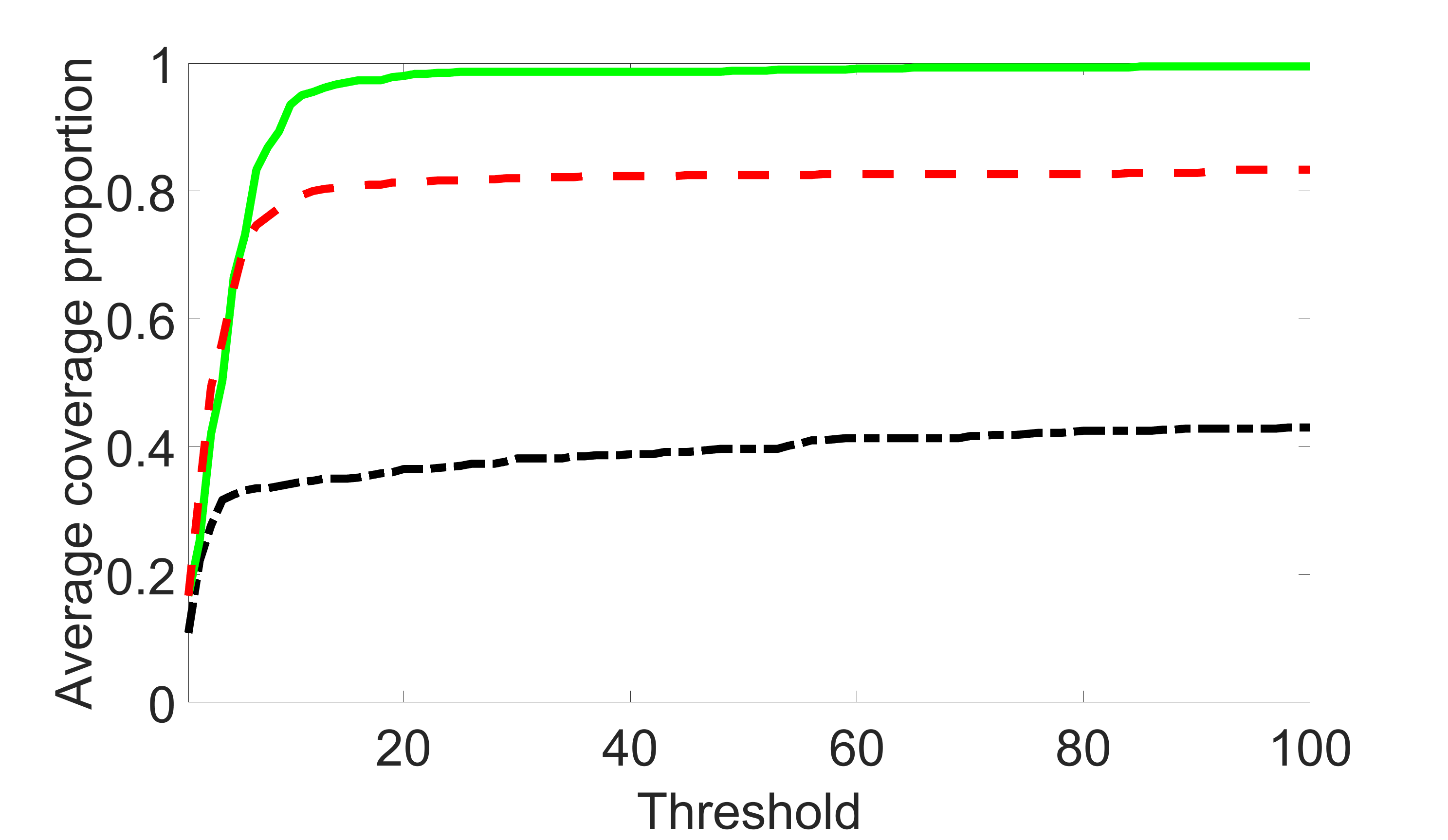
From the plots, one can see that the blockwise joint screening method (blue dotted line) selects and with higher probability compared with the original joint screening method (green solid line). Based on the results, the blockwise joint screening method can better utilize precision variables with block structures to select .
In addition, we evaluate the performance of the two proposed estimation procedure after the first-step screening. For the sizes of and in the screening step, we set for the original joint screening procedure, and for the blockwise joint screening procedure. We report the average MSEs for and when in Table 2. The complete results, in which , , , and , can be found in Table 9 of the supplementary material.
In summary, the blockwise joint screening estimate outperforms the original joint screening estimate when the sample size is small or block size of precision variables is large. For the rest of the scenarios, there are no significant differences between the two methods.
| Proposed | MSE | MSE | Proposed (block) | MSE | MSE |
|---|---|---|---|---|---|
| K=2 | 1.423(0.096) | 0.785(0.009) | K=2 | 1.390(0.090) | 0.793(0.010) |
| K=4 | 1.667(0.096) | 0.815(0.011) | K=4 | 1.548(0.088) | 0.805(0.010) |
| K=6 | 1.955(0.101) | 0.826(0.010) | K=6 | 1.701(0.084) | 0.816(0.009) |
| K=12 | 2.466(0.096) | 0.890(0.039) | K=12 | 2.223(0.129) | 0.838(0.011) |
| K=24 | 2.533(0.164) | 0.847(0.014) | K=24 | 2.136(0.138) | 0.821(0.010) |
| K=52 | 14.650(0.815) | 2.034(0.487) | K=52 | 13.693(0.728) | 1.870(0.459) |
In the supplementary material, we assess the variable screening results for various sparsity levels of instrumental variables in Section 14.2, evaluate the performance of our estimation procedure for different covariances of exposure errors in Section 14.3, and assess the sensitivity of the choices for different sizes of and in Section 14.4.
6 Discussion
This paper aims at mapping the complex GIC pathway for AD. The unique features of the hippocampal morphometry surface measure data motivate us to develop a computationally efficient two-step screening and estimation procedure, which can select biomarkers among more than million observed covariates and estimate the conditional association simultaneously. If there was no unmeasured confounding, then the conditional association we estimate corresponds to the causal effect. This is, however, not the case in the ADNI study because we have unmeasured confounders such as A and tau protein levels. To control for unmeasured confounding and estimate the causal effect, one possible approach is to use the generic variants as potential instrumental variables (e.g. Lin et al., 2015).
There are a number of other important directions for future work. Firstly, the vast majority of AD, known as “polygenic AD”, is influenced by the actions and interactions of multiple genetic variants simultaneously, likely in concert with non-genetic factors, such as environmental exposures and lifestyle choices among many others (Bertram and Tanzi, 2020). Therefore, various types of interaction effects, such as genetic-genetic and imaging-genetic, could be incorporated into the outcome generating model (1). However, this may significantly increase the computation as the dimension of genetic relevant covariates will increase from to more than billion covariates, if we add all the possible imaging-genetics interaction terms. One may consider interaction screening procedures (Hao and Zhang, 2014) as the first-step. Secondly, this study simply removes observations with missingness. Accommodation of missing exposure, confounders and outcome under the proposed model framework is of great practical value and worth further investigation. Thirdly, baseline diagnosis status is an important effect modifier, as the effect of hippocampus shape on behavioral measures can be different across the CN/MCI/AD groups. However, the relatively small sample size in the ADNI study does not allow us to conduct a reliable subgroup analysis. The subgroup analyses are pertinent for further exploration when a larger sample size is available. Fourthly, in the ADNI dataset, there are longitudinal ADAS-13 scores observed at different months as well as other longitudinal behavioral scores obtained from Mini-Mental State Examination and Rey Auditory Verbal Learning Test, which can provide a more comprehensive characterization of the behavioral deficits. Integrating these different scores as a multivariate longitudinal outcome to improve the estimation of the conditional association requires substantial effort for future research. Lastly, one could consider incorporating information from other brain regions. For instance, an entorhinal tau may exist on episodic memory decline through other brain regions, such as the medial temporal lobe (Maass et al., 2018).
Supplementary Material
Supplementary material available online contains detailed derivations and explanations of the main algorithm, ADNI data usage acknowledgement, image and genetic data preprocessing steps, screening results and sensitivity analyses of the ADNI data application with a subgroup analysis including only MCI and AD patients, detailed procedure and results for the SNP-imaging-outcome mediation analyses, additional simulation results, theoretical properties of the proposed procedure including the main theorems, assumptions needed for our main theorems, and proofs of auxiliary lemmas and main theorems.
Acknowledgement
The authors thank the editor, associate editor and referees for their constructive comments, which have substantially improved the paper. Yu was partially supported by the Canadian Statistical Sciences Institute (CANSSI) postdoctoral fellowship and the start-up fund of University of Texas at Arlington. Wang and Kong were partially supported by the Natural Science and Engineering Research Council of Canada and the CANSSI Collaborative Research Team Grant. Zhu was partially supported by the NIH-R01-MH116527.
Supplementary Material for
“Mapping the Genetic-Imaging-Clinical Pathway with Applications to Alzheimer’s Disease”
Dengdeng Yu
Department of Mathematics, University of Texas at Arlington
Linbo Wang
Department of Statistical Sciences, University of Toronto
Dehan Kong
Department of Statistical Sciences, University of Toronto
Hongtu Zhu
Department of Biostatistics, University of North Carolina, Chapel Hill
for the Alzheimer’s Disease Neuroimaging Initiative
111
Data used in preparation of this article were obtained from the Alzheimer’s Disease
Neuroimaging Initiative (ADNI) database (adni.loni.usc.edu). As such, the investigators within the ADNI contributed to the design and implementation of ADNI and/or provided data but did not participate in analysis or writing of this report. A complete listing of ADNI investigators can be found at: http://adni.loni.usc.edu/wp-content/uploads/how_to_apply/ADNI_Acknowledgement_List.pdf.
The supplementary file is organized as follows. The detailed description of the main algorithm is included in Section 7. We include the ADNI data usage acknowledgement in Section 8 and image and genetic data preprocessing steps in Section 9. In Section 10, we list the screening results of ADNI data applications. Section 11 examines the sensitivity of the estimate from the ADNI data application by varying the relative sizes of and . Section 12 includes a subgroup analysis including only the mild cognitive impairment (MCI) and Alzheimer’s disease (AD) patients. We include the detailed SNP-imaging-outcome mediation analysis procedure and results in Section 13. In Section 14, we list additional simulation results. The theoretical properties including the main theorems of our procedure are included in Section 15. We state the assumptions needed for the main theorems in Section 16. In Section 17, we include the auxiliary lemmas needed for the theorems and their proofs. We give the detailed proofs of our main theorems in Section 18.
7 Description and derivation of Algorithm 1
To solve the minimization problem (3) of the main paper, we utilize the Nesterov optimal gradient method (Nesterov, 1998), which has been widely used in solving optimization problems for non-smooth and non-convex objective functions (Beck and Teboulle, 2009; Zhou and Li, 2014).
Before we introduce Nesterov’s gradient algorithm, we first state two propositions on shrinkage thresholding formulas (Beck and Teboulle, 2009; Cai et al., 2010).
Proposition 1.
For a given matrix with singular value decomposition , where with being ’s singular values, the optimal solution to
share the same singular vectors as and its singular values are for , where .
Proposition 2.
For vectors and , the optimal solution to
is for , where denotes the sign of the number.
The Nestrov’s gradient method utilizes the first-order gradient of the objective function to produce the next iterate based on the current search point. Differed from the standard gradient descent algorithm, the Nesterov’s gradient algorithm uses two previous iterates to generate the next search point by extrapolating, which can dramatically improve the convergence rate. The Nesterov’s gradient algorithm for problem (3) is presented as follows. Denote and , where and . We also define
where denotes the first-order gradient of with respect to . We define
with , . Here and are interpolations between and , and and respectively, which will be defined below; denotes all terms that are irrelevant to , and is a suitable step size. Given previous search points and , the next search points and would be the minimizer of . For the search points and , they can be generated by linearly extrapolating two previous algorithmic iterates. A key advantage of using the Nestrov gradient method is that it has an explicit solution at each iteration. In fact, minimizing can be divided into two sub-problems, minimizing and , respectively. These sub-problems can be solved by the shrinkage thresholding formulas in Propositions 1 and 2, respectively.
Let where is for . Define and . For a given vector , is defined as , where . Similarly, is obtained by taking the sign of componentwisely. For a given pair of tuning parameters and , (3) can be solved by Algorithm 1.
-
1.
Initialize: , , and ,
. -
2.
Repeat (a) to (f) until the objective function converges:
-
(a)
,
; -
(b)
;
; -
(c)
Singular value decomposition: ;
-
(d)
,
; -
(e)
,
; -
(f)
.
-
(a)
In particular, step 2(a) predicts search points and by linear extrapolations from the solutions of previous two iterates, where is a scalar sequence that plays a critical role in the extrapolation. This sequence is updated in step 2(f) as in the original Nesterov method. Next, steps 2(b) – 2(d) perform gradient descent from the current search points to obtain the optimal solutions at current iteration. Specifically, the gradient descent is based on minimizing , the first-order approximation to the loss function, at the current search points and . This minimization problem is tackled by minimizing two sub-problems by the shrinkage thresholding formulas in Propositions 1 and 2 respectively, as mentioned above. Finally, step 2(e) forces the descent property of the next iterate.
A sufficient condition for the convergence of and is that the step size should be smaller than or equal to , where is the smallest Lipschitz constant of the function (Beck and Teboulle, 2009). In our case, is equal to , where denotes the largest eigenvalue of a matrix.
8 Data usage acknowledgement
Data used in the preparation of this article were obtained from the Alzheimer’s Disease Neuroimaging Initiative (ADNI) database (adni.loni.usc.edu). The ADNI was launched in 2003 as a public-private partnership, led by Principal Investigator Michael W. Weiner, MD. The primary goal of ADNI has been to test whether serial magnetic resonance imaging (MRI), positron emission tomography (PET), other biological markers, and clinical and neuropsychological assessment can be combined to measure the progression of mild cognitive impairment and early Alzheimer’s disease. For up-to-date information, see www.adni-info.org.
Data collection and sharing for this project was funded by the Alzheimer’s Disease Neuroimaging Initiative (ADNI) (National Institutes of Health Grant U01 AG024904) and DOD ADNI (Department of Defense award number W81XWH-12-2-0012). ADNI is funded by the National Institute on Aging, the National Institute of Biomedical Imaging and Bioengineering, and through generous contributions from the following: AbbVie, Alzheimer’s Association; Alzheimer’s Drug Discovery Foundation; Araclon Biotech; BioClinica, Inc.; Biogen; Bristol-Myers Squibb Company; CereSpir, Inc.; Cogstate; Eisai Inc.; Elan Pharmaceuticals, Inc.; Eli Lilly and Company; EuroImmun; F. Hoffmann-La Roche Ltd and its affiliated company Genentech, Inc.; Fujirebio; GE Healthcare; IXICO Ltd.; Janssen Alzheimer Immunotherapy Research & Development, LLC.; Johnson & Johnson Pharmaceutical Research & Development LLC.; Lumosity; Lundbeck; Merck & Co., Inc.; Meso Scale Diagnostics, LLC.; NeuroRx Research; Neurotrack Technologies; Novartis Pharmaceuticals Corporation; Pfizer Inc.; Piramal Imaging; Servier; Takeda Pharmaceutical Company; and Transition Therapeutics. The Canadian Institutes of Health Research is providing funds to support ADNI clinical sites in Canada. Private sector contributions are facilitated by the Foundation for the National Institutes of Health (www.fnih.org). The grantee organization is the Northern California Institute for Research and Education, and the study is coordinated by the Alzheimer’s Therapeutic Research Institute at the University of Southern California. ADNI data are disseminated by the Laboratory for Neuro Imaging at the University of Southern California.
9 Image and genetic data preprocessing
9.1 Image data preprocessing
The hippocampus surface data were preprocessed from the raw MRI data, which were collected across a variety of 1.5 Tesla MRI scanners with protocols individualized for each scanner. Standard T1-weighted images were obtained by using volumetric 3-dimensional sagittal MPRAGE or equivalent protocols with varying resolutions. The typical protocol includes: inversion time (TI) = 1000 ms, flip angle = 8o, repetition time (TR) = 2400 ms, and field of view (FOV) = 24 cm with a acquisition matrix in the , , and dimensions yielding a voxel size of mm3. We adopted a surface fluid registration based hippocampal subregional analysis package (Shi et al., 2013), which uses isothermal coordinates and fluid registration to generate one-to-one hippocampal surface registration for surface statistics computation. It introduced two cuts on a hippocampal surface to convert it into a genus zero surface with two open boundaries. The locations of the two cuts were at the front and back of the hippocampal surface. By using conformal parameterization, it essentially converts a 3D surface registration problem into a 2D image registration problem. The flow induced in the parameter domain establishes high-order correspondences between 3D surfaces. Finally, the radial distance was computed on the registered surface. This software package and associated image processing methods have been adopted and described in Wang et al. (2011).
9.2 Genetic data preprocessing
For the genetic data, we applied the following preprocessing technique to the subjects in ADNI1 study. The first line quality control steps include (i) call rate check per subject and per single nucleotide polymorphism (SNP) marker, (ii) gender check, (iii) sibling pair identification, (iv) the Hardy-Weinberg equilibrium test, (v) marker removal by the minor allele frequency, and (vi) population stratification. The second line preprocessing steps include removal of SNPs with (i) more than 5 missing values, (ii) minor allele frequency smaller than 10, and (iii) Hardy-Weinberg equilibrium -value . The 503,892 SNPs obtained from 22 autosomes were included for further processing. MACH-Admix software (http://www.unc.edu/ yunmli/MaCH-Admix/) (Liu et al., 2013) is applied on all the subjects to perform genotype imputation, using 1000G Phase I Integrated Release Version 3 haplotypes (http://www.1000genomes.org) (Consortium et al., 2012) as reference panel. Quality control was also conducted after imputation, excluding markers with (i) low imputation accuracy (based on imputation output ), (ii) Hardy-Weinberg equilibrium -value , and (iii) minor allele frequency .
10 Screening results of ADNI data applications
In Table 3, we list the top SNPs selected through the blockwise joint screening procedure corresponding to left and right hippocampi respectively.
| Left hippocampi | Right hippocampi | ||
|---|---|---|---|
| Chromesome number | SNP name | Chromesome number | SNP name |
| 19 | rs429358 | 19 | rs429358 |
| 7 | rs1016394 | 19 | rs10414043 |
| 19 | rs10414043 | 14 | 14:25618120:G_GC |
| 7 | rs1181947 | 19 | rs7256200 |
| 19 | rs7256200 | 14 | rs41470748 |
| 22 | rs134828 | 19 | rs73052335 |
| 19 | rs73052335 | 14 | 14:25613747:G_GT |
| 7 | 7:101403195:C_CA | 19 | rs157594 |
| 19 | rs157594 | 14 | rs72684825 |
| 13 | rs12864178 | 19 | rs769449 |
| 19 | rs769449 | 6 | rs9386934 |
| 2 | rs13030626 | 6 | rs9374191 |
| 19 | rs56131196 | 19 | rs56131196 |
| 2 | rs13030634 | 6 | rs9372261 |
| 19 | rs4420638 | 19 | rs4420638 |
| 2 | rs11694935 | 6 | rs73526504 |
| 19 | rs111789331 | 19 | rs111789331 |
| 2 | rs11696076 | 14 | rs187421061 |
| 19 | rs66626994 | 19 | rs66626994 |
| 2 | rs11692218 | 13 | rs342709 |
We plot similar figures as the Manhattan plot for , , and in Figure 7. Unlike the conventional Manhattan plots, where genomic coordinates are displayed along the x-axis, with the negative logarithm of the association p-value for each SNP displayed on the y-axis, in our analysis, we do not have the p-values. So in these figures, the y-axis represents the magnitude of , , and and the horizontal dashed line represents the threshold values (Panel (a)), ((Panel (b)), ((Panel (c)) and ((Panel (d)). In Panels (c) and (d), the left and right figures represent the left and right hippocampi, respectively. The SNPs with , , and greater than or equal to , , and , hence being selected by , , and respectively, are highlighted with red diamond symbols.

11 Sensitivity analysis of ADNI data applications
In our analysis, we set and the same sizes, following the convention that the size of screening set is determined only by the sample size (Fan and Lv, 2008), which is the same for and . To assess the sensitivity of our results to this choice, we conduct sensitivity analyses varying the relative sizes of and in the joint screening procedure. For simplicity, we only consider the joint screening procedure proposed in Section 3.3. Figure 8 lists the estimate corresponding to the left hippocampi (left part) and the right hippocampi (right part) using . Denote the estimates corresponding to by , , respectively. We set . The estimates , and are plotted in Figure 8 (a), (b) and (c) correspondingly. In addition, we consider but . Denote the corresponding estimate by . We plot in Figure 8 (d).
Furthermore, by defining the relative risk of an estimate as , we report the relative risks of three estimates , and in Table 4.
| Left hippocampi | Right hippocampi | |
|---|---|---|
| 0.0022 | 0.1074 | |
| 0.2938 | 0.0907 | |
| 0.0611 | 0.0927 |
| Number of negative entries | Left hippocampi | Right hippocampi |
|---|---|---|
| 15,000 | 15,000 | |
| 15,000 | 15,000 | |
| 14,600 | 15,000 | |
| 15,000 | 15,000 |
To summarize, the estimate is not very sensitive against the choices of and except for the left hippocampi when and . In fact, as shown in Table 5, when , for the left hippocampi, there are entries are non-negative. We believe it may be due to some confounder variables being missed in the screening step. For instance, we find that rs157582, a previously identified risk loci for Alzheimer’s disease (Guo et al., 2019) is adjusted in estimating , and except for . But in general, as demonstrated in Figure 8, the estimate s are similar among different choices of and .
12 Subgroup analysis ADNI data applications
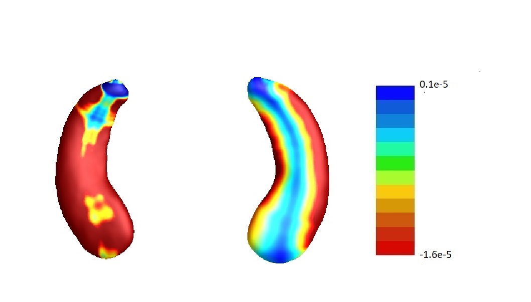
We repeat the analysis on the MCI and AD subjects. The estimates corresponding to each part of the hippocampus onto a representative hippocampal surface are plotted in Figure 9(a). We have also plotted the hippocampal subfield (Apostolova et al., 2006) in Figure 9(b). The results are similar to the complete data analysis including all the subjects. For example, from these plots, we can see that entries of corresponding to left and all the entries of corresponding to right hippocampi are negative. This implies that the radial distances of each pixel of both hippocampi are mostly negatively associated with the ADAS-13 score, which depicts the severity of behavioral deficits. Furthermore, the subfields with the strongest associations are still mostly CA1 and subiculum.

13 Results for mediation analyses
We perform the SNP-imaging-outcome mediation analyses following the same procedure as in Bi et al. (2017). In specific, we regress the imaging measures against SNPs in the first step to search for the pairs of intermediate imaging measures and genetic variants. Then the behaviour outcome is fit against each candidate genetic variant to identify direct and significant influence. In the last step, the behaviour outcome is fit against identified genetic variant and its associated intermediate imaging measure simultaneously. A mediation relationship is built if a) the genetic variant is significant in both first and second steps, b) the intermediate imaging measure is significant in the last step, and c) the genetic variant has a smaller coefficient in the last step compared with the second step. Note that the total effect of the genetic variant in the second step should be the summation of direct and indirect effects which motivates the criterion c) of coefficient comparison. Note that, the total effect may not always be greater than the direct effect in the last step when the direct and indirect effects have opposite signs, while the causal inference tool proposed in this paper does not have this problem. Similar to Bi et al. (2017), we try to identify the pairs of SNP and imaging measure, for which the direct effect of SNP on behavioral outcome, the effect of SNP on imaging measure and the effect of imaging measure on the behavioral outcome are all significant. However, there is no SNP with at least one paired imaging measure (i.e. hippocampal imaging pixel) being significant. Therefore, there is no evidence for the mediating relationship of SNP-imaging-outcome from our analysis.
14 Additional results for simulation studies
In this section, we list additional simulation results. In particular, Figures 10 – 14 present the screening results for Section 5.1 with , , , and , respectively. Section 14.1 presents the sensitivity and specificity analyses for Section 5.2, where the detailed definitions of sensitivity and specificity can be found here. Section 14.2 presents an additional simulation study considering various sparsity levels of instrumental variables. Section 14.3 presents an additional simulation study considering different covariances of exposure errors. Section 14.4 conducts an additional simulation study by varying the relative sizes of and . Section 14.5 lists additional screening and estimation results for Section 5.3 of the main article.

outcome, weak exposure
outcome, medium exposure
outcome, strong exposure
outcome, zero exposure
outcome, zero exposure

outcome, zero exposure
outcome, weak exposure
outcome, medium exposure
outcome, strong exposure

outcome, zero exposure

outcome, zero exposure

outcome, zero exposure

outcome, weak exposure
outcome, medium exposure
outcome, strong exposure
outcome, zero exposure
outcome, zero exposure
outcome, zero exposure
outcome, weak exposure

outcome, medium exposure
outcome, strong exposure

outcome, zero exposure
outcome, zero exposure

outcome, zero exposure
outcome, weak exposure
outcome, medium exposure
outcome, strong exposure
outcome, zero exposure

outcome, zero exposure
outcome, zero exposure
14.1 Sensitivity and specificity analyses of simulation
In this subsection, we report the sensitivity and specificity of the estimates. The sensitivity (true positive rate) is defined as , i.e. the proportion of variables in the oracle adjustment set that are selected by our estimation procedure. The specificity (true negative rate) is defined as , i.e. the proportion of variables not in the oracle adjustment set that are not selected by our estimation procedure. Furthermore, we define the instrumental specificity as , i.e. the proportion of variables in the instrumental set that are not selected by our estimation procedure.
| n = 500 | Sensitivity | Instrumental specificity | Specificity | MSE | MSE |
|---|---|---|---|---|---|
| = 1.0 | |||||
| Oracle | 1.000(0.000) | 1.000(0.000) | 1.000(0.000) | 0.036(0.002) | 0.553(0.005) |
| Proposed | 0.833(0.000) | 0.293(0.020) | 0.998(0.000) | 0.303(0.008) | 0.574(0.006) |
| No Lasso | 1.000(0.000) | 0.000(0.000) | 0.985(0.000) | 1.740(0.078) | 0.693(0.013) |
| = 0.5 | |||||
| Oracle | 1.000(0.000) | 1.000(0.000) | 1.000(0.000) | 0.006(0.000) | 0.340(0.004) |
| Proposed | 0.897(0.008) | 0.217(0.017) | 0.999(0.000) | 0.191(0.005) | 0.345(0.004) |
| No Lasso | 1.000(0.000) | 0.000(0.000) | 0.985(0.000) | 0.372(0.017) | 0.371(0.004) |
In the simulation studies, we report the results for the case , which is close to the sample size in the real data. From Table 6, one can see that the second step can only regularize out some of the instrumental variables. We guess there may be a better tuning method, which can regularize out more instrumental variables, while still keep the confounders and prevision variables in the model. We leave this as future research. Nevertheless, one can also see from Table 6 that although the proposed method may not remove all of the instrumental variables, eliminating even just some of the instruments greatly reduce the MSEs of both and , compared to the method where we do not impose -regularization on in the second-step estimation (denoted by the “No Lasso” method). In addition, the estimation of is reasonably good compared to the oracle estimates as shown in Table 1 of the main article.
14.2 Screening under different sparsity levels
We also consider different sparsity levels in the simulation. It is particularly of interest for our study since when more instrumental variables than confounders and precision variables exist, which could be the case in an imaging-genetic study, the robustness of the proposed method may be undermined. As discussed before, to reduce bias and increase the statistical efficiency of the estimated , the ideal adjustment set should include all confounders and precision variables while excluding instrumental variables and irrelevant variables. In particular, we consider three scenarios where the sizes of instrumental variables are the same, twice, and eight times of the size of confounders and precision variables .
We set and the settings for and remain the same as before: is as in Figure 4(a), and is as in Figure 4(b). Further we set , where , , , , , , and for and . Here is a positive integer. We set , , , , , , and for and . In this setting, we have , , and . Note that . For , we let and , and consider three different sparsity levels that . The complete screening results can be found in Figures 16 – 21.
Specifically, as summarized in Figure 15, when the number of instrumental variables is much larger than that of confounders and precision variables, the size of is larger than the number of covariates kept in the first screening step. And in this case, our results show that the screening step may include many instrumental variables, while missing some confounders and precision variables. This may deteriorate the accuracy and efficiency of the second step estimation.

outcome, weak exposure
outcome, medium exposure
outcome, strong exposure
outcome, zero exposure
outcome, zero exposure
outcome, zero exposure
outcome, weak exposure
outcome, medium exposure
outcome, strong exposure
outcome, zero exposure
outcome, zero exposure
outcome, zero exposure
outcome, weak exposure
outcome, medium exposure
outcome, strong exposure
outcome, zero exposure
outcome, zero exposure
outcome, zero exposure
outcome, weak exposure
outcome, medium exposure
outcome, strong exposure
outcome, zero exposure
outcome, zero exposure
outcome, zero exposure
outcome, weak exposure
outcome, medium exposure
outcome, strong exposure
outcome, zero exposure
outcome, zero exposure
outcome, zero exposure
outcome, weak exposure
outcome, medium exposure
outcome, strong exposure
outcome, zero exposure
outcome, zero exposure
outcome, zero exposure
14.3 Screening and estimation under different covariances of exposure errors
We also consider various exposure errors in the simulation. We use the same setting as Section 5.1 of the main paper but taking three different covariance structures of exposure errors . In particular, the random error is independently generated from , where we set the standard deviations of all elements in to be and the correlation between and to be for with . We consider three scenarios that , , and , and report the selected covariates from the screening step. We consider or and fix the sample size . The complete screening results can be found in Figure 5 as well as Figures 10, 23 – 26 here ( is set to be in Section 5.1 of the main paper).
Specifically, as summarized in Figure 22, when increases, the average coverage proportion for the index set does not change too much.
In addition, we evaluate the performance of our estimation procedure after the first-step screening. For the size of in the screening step, we set , so that for sample size . We report the mean squared errors (MSEs) for and defined as and , respectively.
Table 7 summarizes the average MSEs for and among 100 Monte Carlo runs. We can see that the MSE decreases with increases. As nuclear norm penalization estimation procedure can be regarded as one way of spatial smoothing, the large correlations among actually help with the spatial smoothing, and thus we have better estimation accuracy when increases.
| MSE | MSE | MSE | MSE | ||
|---|---|---|---|---|---|
| 0.986(0.099) | 0.802(0.011) | 0.397(0.042) | 0.701(0.006) | ||
| 0.496(0.021) | 0.667(0.005) | 0.276(0.009) | 0.528(0.005) | ||
| 0.252(0.010) | 0.439(0.007) | 0.097(0.006) | 0.305(0.004) |
outcome, weak exposure
outcome, medium exposure

outcome, strong exposure
outcome, zero exposure
outcome, zero exposure
outcome, zero exposure
outcome, weak exposure
outcome, medium exposure
outcome, strong exposure

outcome, zero exposure
outcome, zero exposure
outcome, zero exposure

outcome, weak exposure
outcome, medium exposure
outcome, strong exposure

outcome, zero exposure
outcome, zero exposure
outcome, zero exposure
outcome, weak exposure
outcome, medium exposure
outcome, strong exposure
outcome, zero exposure
outcome, zero exposure
outcome, zero exposure
14.4 Screening and estimation under different sizes of and
In addition, we conduct a similar study following the same setting as described in Section 5.1 of the main paper, where and . We use here since it is close to the number of observations in the real data analysis. Specifically, as summarized in Figures 27 and 28, when the ratio of is taken as or , the performances of the proposed joint screening method are quite similar to each other. By comparing them with Figure 11, where , the performances of the screening step results are quite similar.
outcome, weak exposure
outcome, medium exposure
outcome, strong exposure
outcome, zero exposure
outcome, zero exposure
outcome, zero exposure
outcome, weak exposure
outcome, medium exposure
outcome, strong exposure
outcome, zero exposure
outcome, zero exposure
outcome, zero exposure
Furthermore, we evaluate the performance of our estimation procedure after the first-step screening. For the size of in the screening step, we set , so that for sample size . We report the mean squared errors (MSEs) for and defined as and , respectively. As summarized in Table 8, the average MSEs for and among 100 Monte Carlo runs are all similar to each other for the different choices of and . Therefore, depending on the prior knowledge about the sizes and strengths of signals of confounding, precision and instrumental variables, one may choose and differently, though the estimations of appear to be similar among the different choices.
| MSE | MSE | |
|---|---|---|
| 0.5 | 0.301(0.008) | 0.567(0.005) |
| 1.0 | 0.303(0.008) | 0.574(0.006) |
| 2.0 | 0.302(0.008) | 0.574(0.006) |
14.5 Screening and estimation using blockwise joint screening
In this section, we list additional screening and estimation results for Section 5.3 of the main article. In particular, the results for the screening step, in which , , , and , can be found in Figures 29 – 46. The complete results for the second step estimation, in which , , , and , can be found in Table 9.
outcome, weak exposure
outcome, medium exposure
outcome, strong exposure

outcome, zero exposure
outcome, zero exposure
outcome, zero exposure
outcome, zero exposure
outcome, weak exposure
outcome, medium exposure
outcome, strong exposure
outcome, zero exposure
outcome, zero exposure
outcome, zero exposure
outcome, zero exposure
outcome, weak exposure
outcome, medium exposure
outcome, strong exposure

outcome, zero exposure
outcome, zero exposure
outcome, zero exposure
outcome, zero exposure
outcome, weak exposure
outcome, medium exposure
outcome, strong exposure
outcome, zero exposure
outcome, zero exposure
outcome, zero exposure
outcome, zero exposure
outcome, weak exposure
outcome, medium exposure
outcome, strong exposure
outcome, zero exposure
outcome, zero exposure
outcome, zero exposure
outcome, zero exposure
outcome, weak exposure
outcome, medium exposure
outcome, strong exposure
outcome, zero exposure
outcome, zero exposure
outcome, zero exposure
outcome, zero exposure
outcome, weak exposure
outcome, medium exposure
outcome, strong exposure

outcome, zero exposure

outcome, zero exposure
outcome, zero exposure
outcome, zero exposure
outcome, weak exposure
outcome, medium exposure
outcome, strong exposure
outcome, zero exposure
outcome, zero exposure
outcome, zero exposure
outcome, zero exposure
outcome, weak exposure
outcome, medium exposure
outcome, strong exposure

outcome, zero exposure
outcome, zero exposure
outcome, zero exposure
outcome, zero exposure
outcome, weak exposure
outcome, medium exposure
outcome, strong exposure
outcome, zero exposure
outcome, zero exposure
outcome, zero exposure
outcome, zero exposure
outcome, weak exposure
outcome, medium exposure
outcome, strong exposure
outcome, zero exposure
outcome, zero exposure
outcome, zero exposure
outcome, zero exposure
outcome, weak exposure
outcome, medium exposure
outcome, strong exposure
outcome, zero exposure
outcome, zero exposure
outcome, zero exposure
outcome, zero exposure
outcome, weak exposure

outcome, medium exposure
outcome, strong exposure

outcome, zero exposure
outcome, zero exposure
outcome, zero exposure
outcome, zero exposure
outcome, weak exposure
outcome, medium exposure
outcome, strong exposure

outcome, zero exposure
outcome, zero exposure
outcome, zero exposure
outcome, zero exposure
outcome, weak exposure
outcome, medium exposure
outcome, strong exposure
outcome, zero exposure
outcome, zero exposure
outcome, zero exposure
outcome, zero exposure
outcome, weak exposure
outcome, medium exposure
outcome, strong exposure
outcome, zero exposure
outcome, zero exposure
outcome, zero exposure
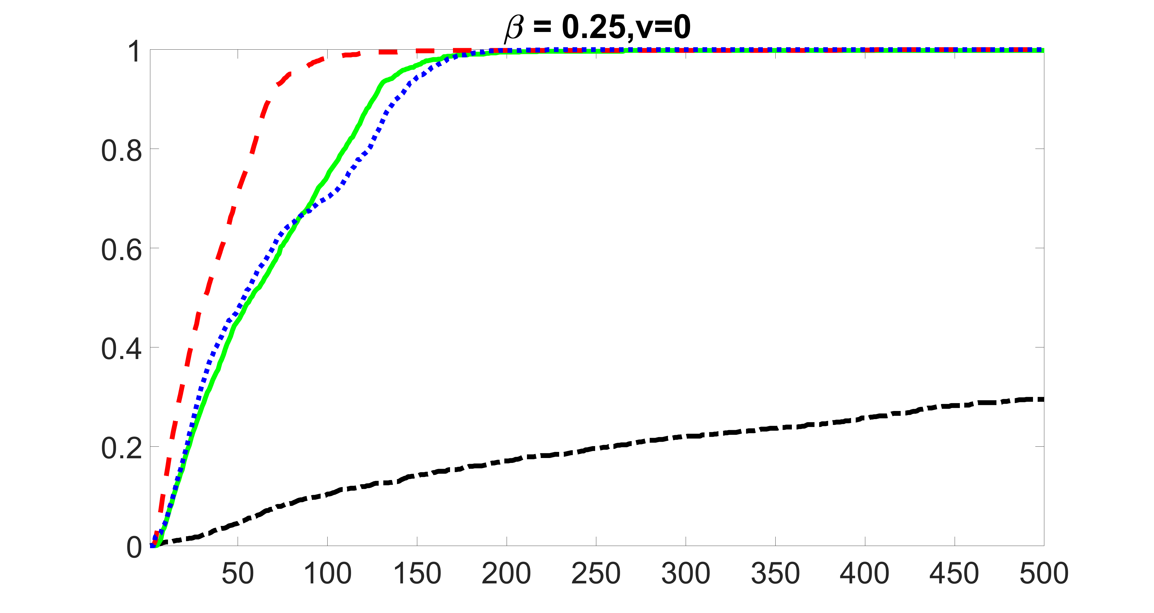
outcome, zero exposure
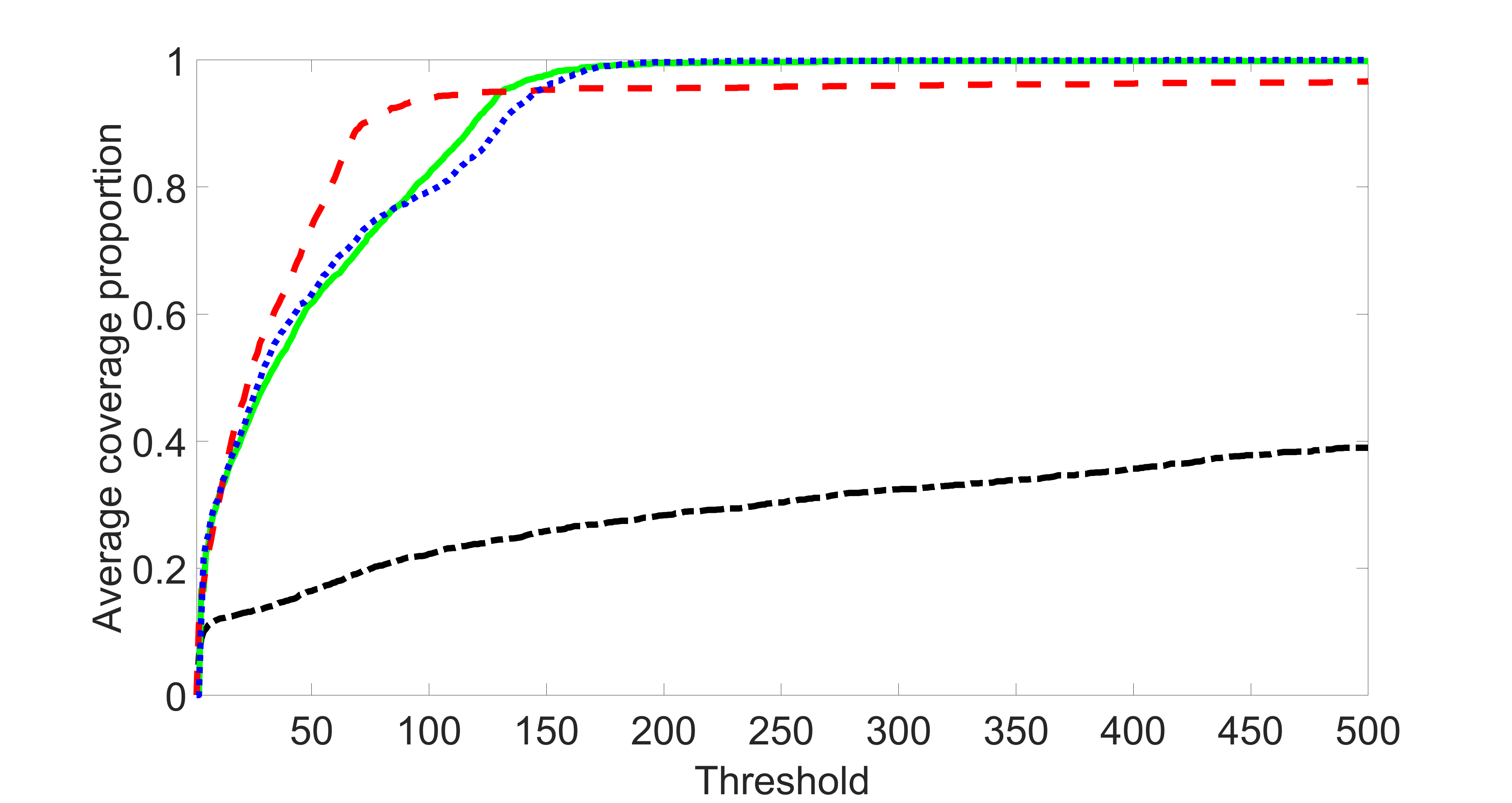
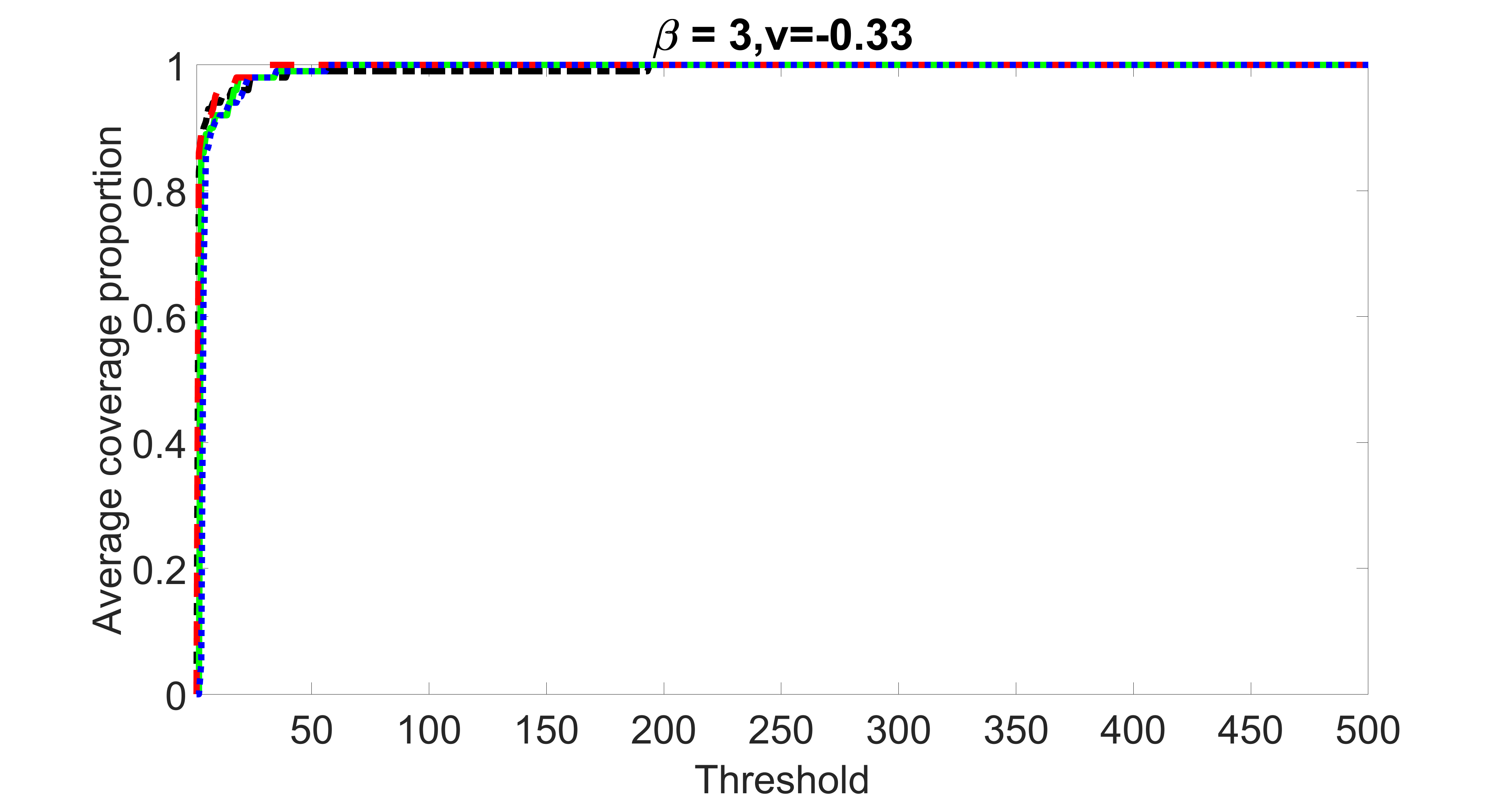
outcome, weak exposure
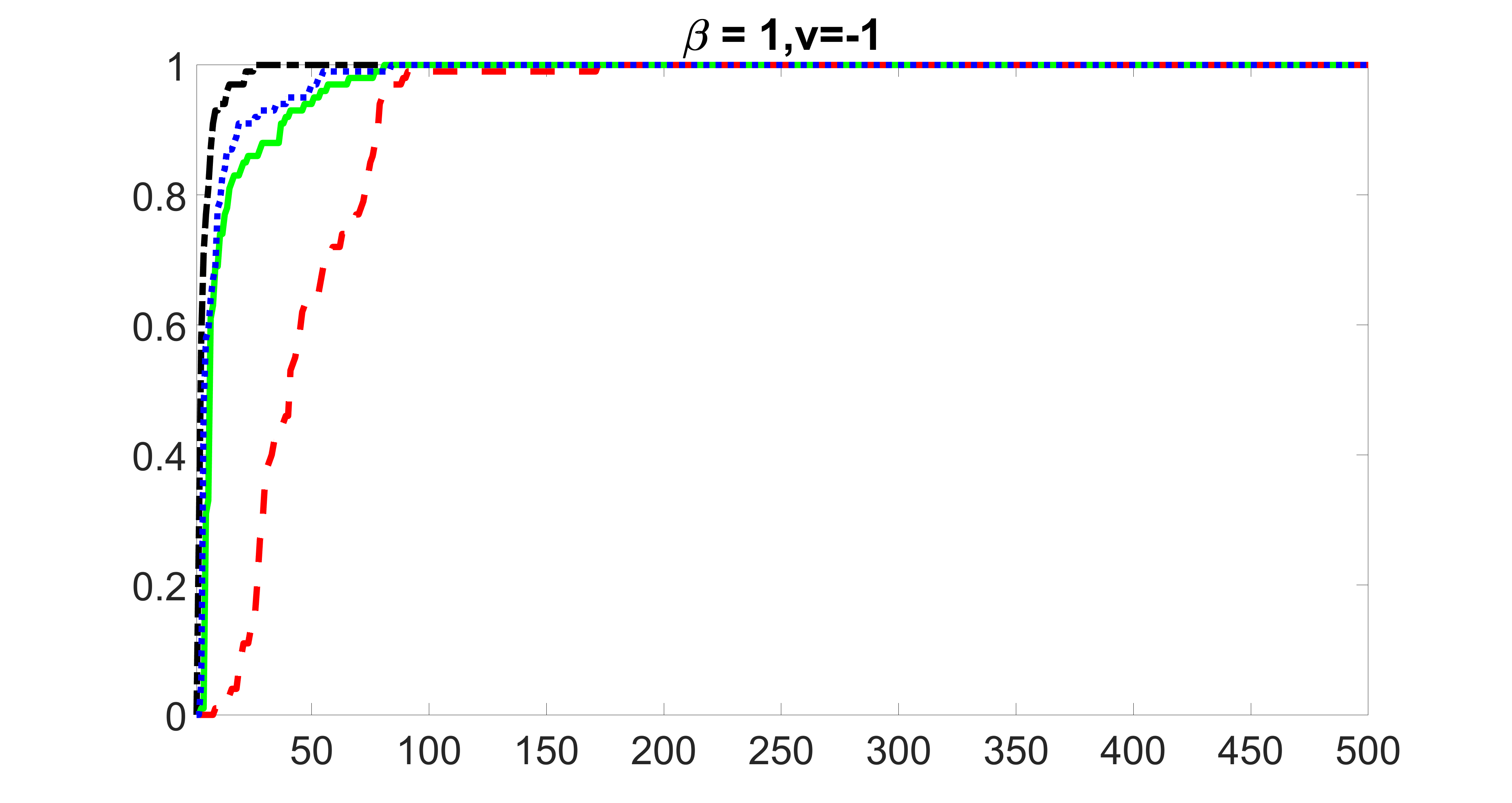
outcome, medium exposure
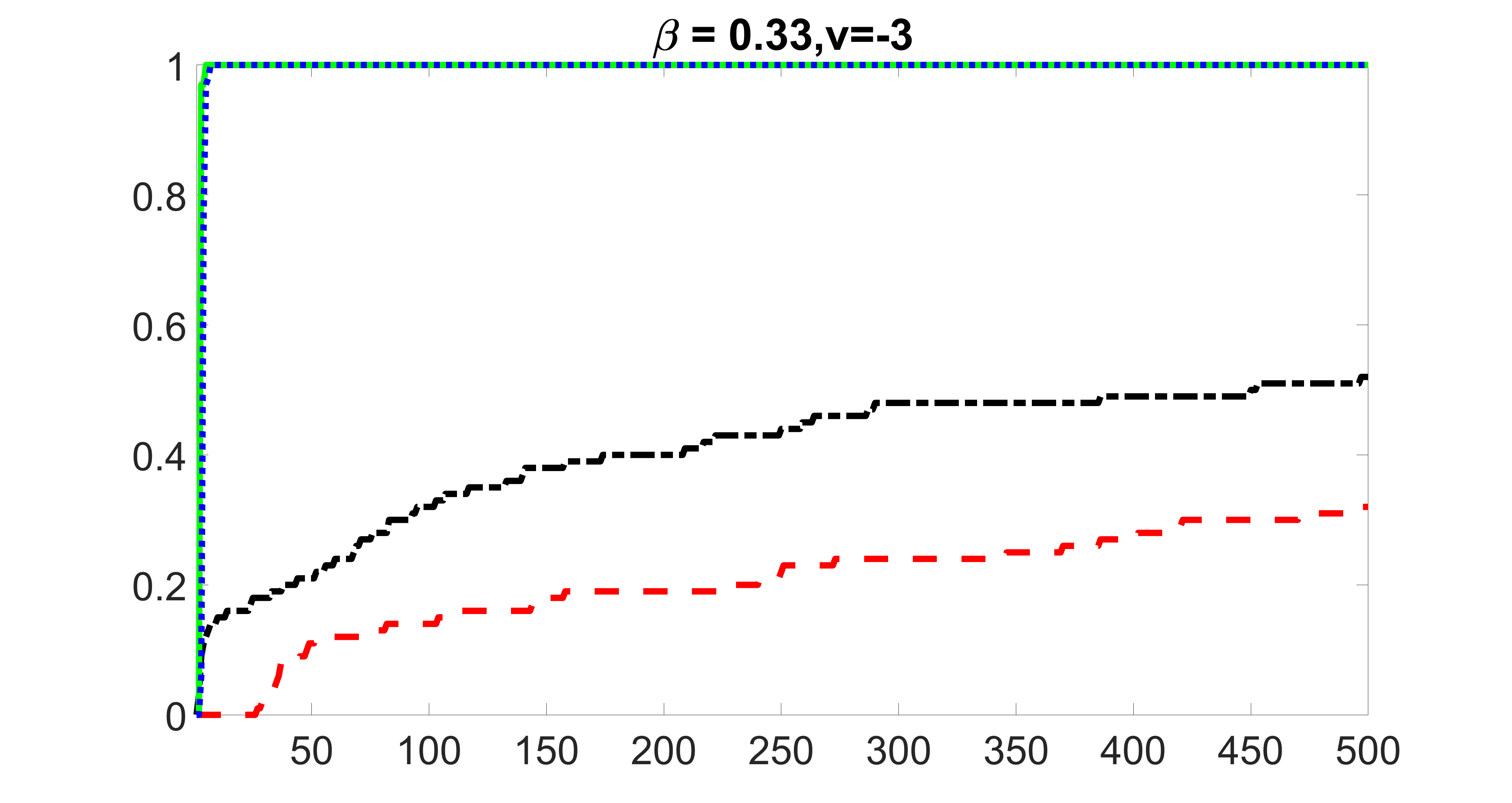
outcome, strong exposure
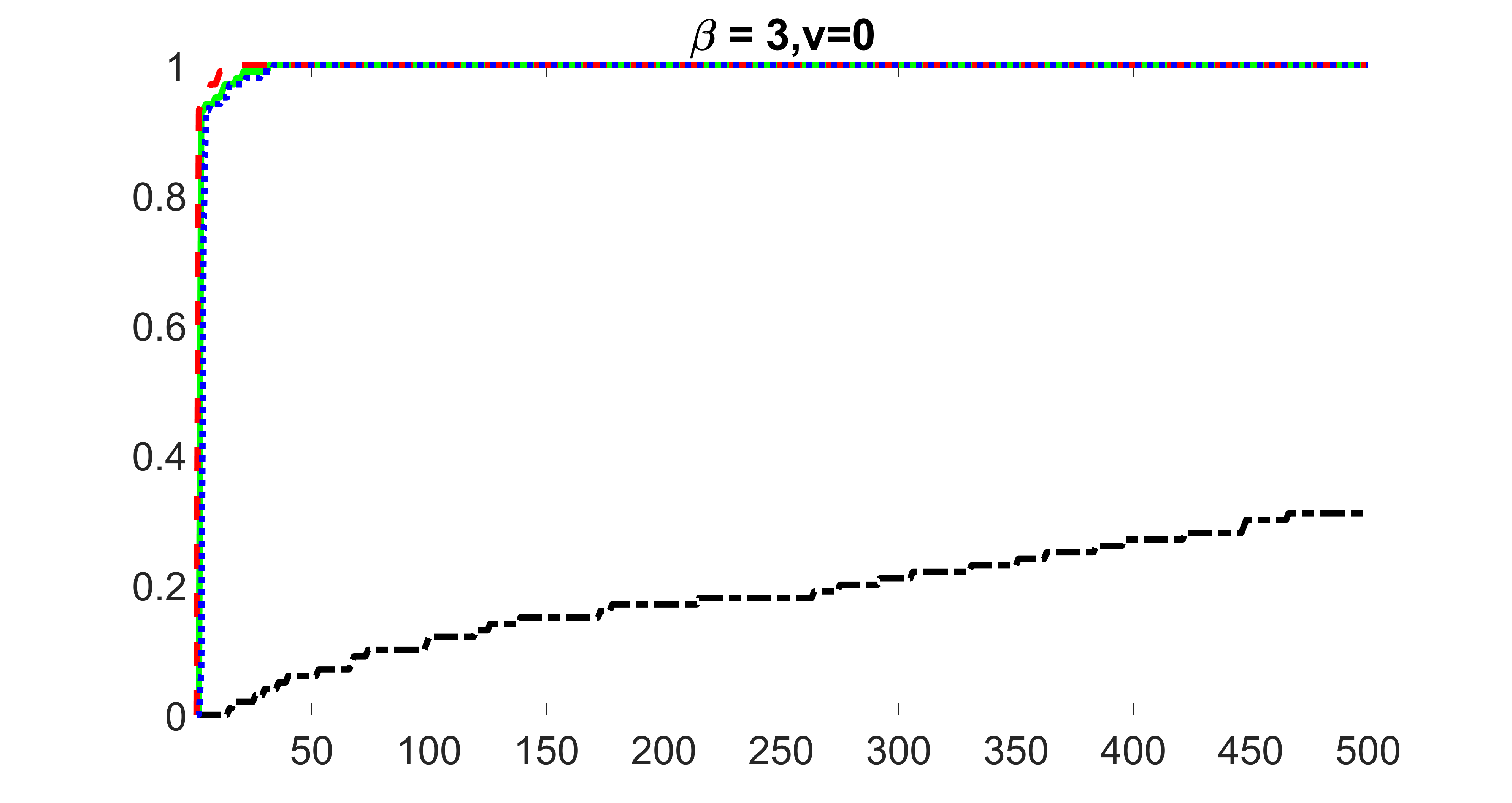
outcome, zero exposure
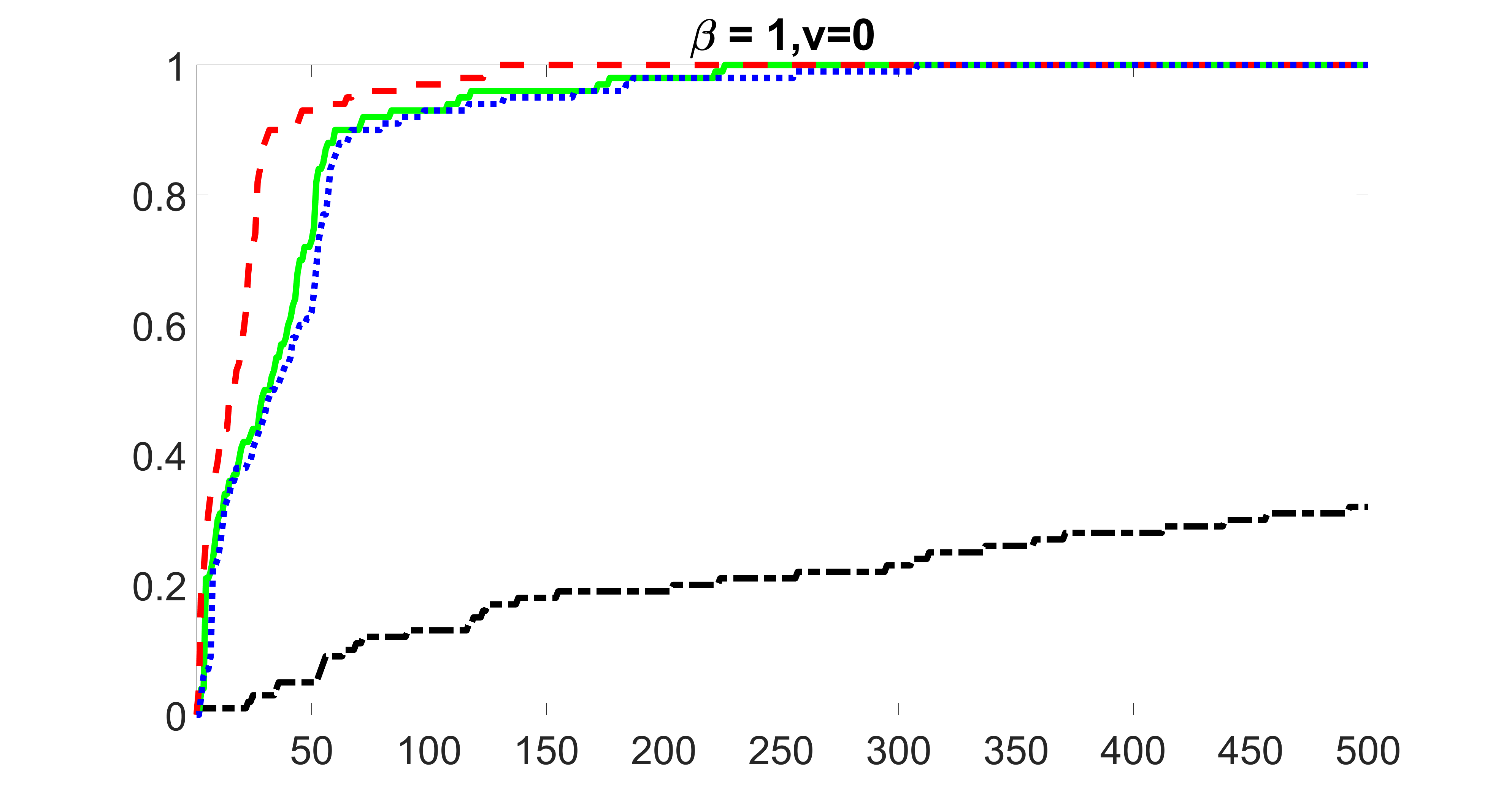
outcome, zero exposure
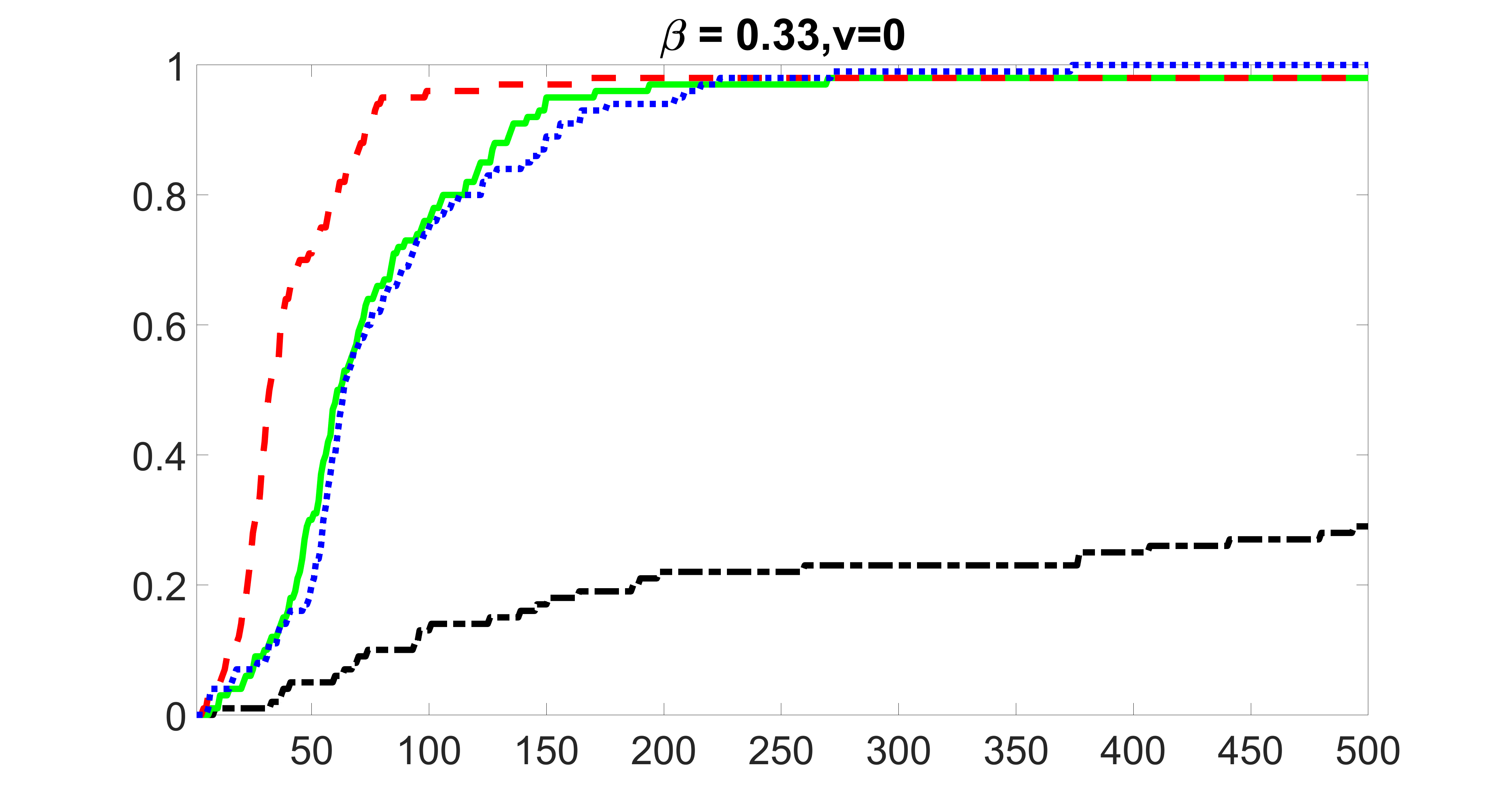
outcome, zero exposure
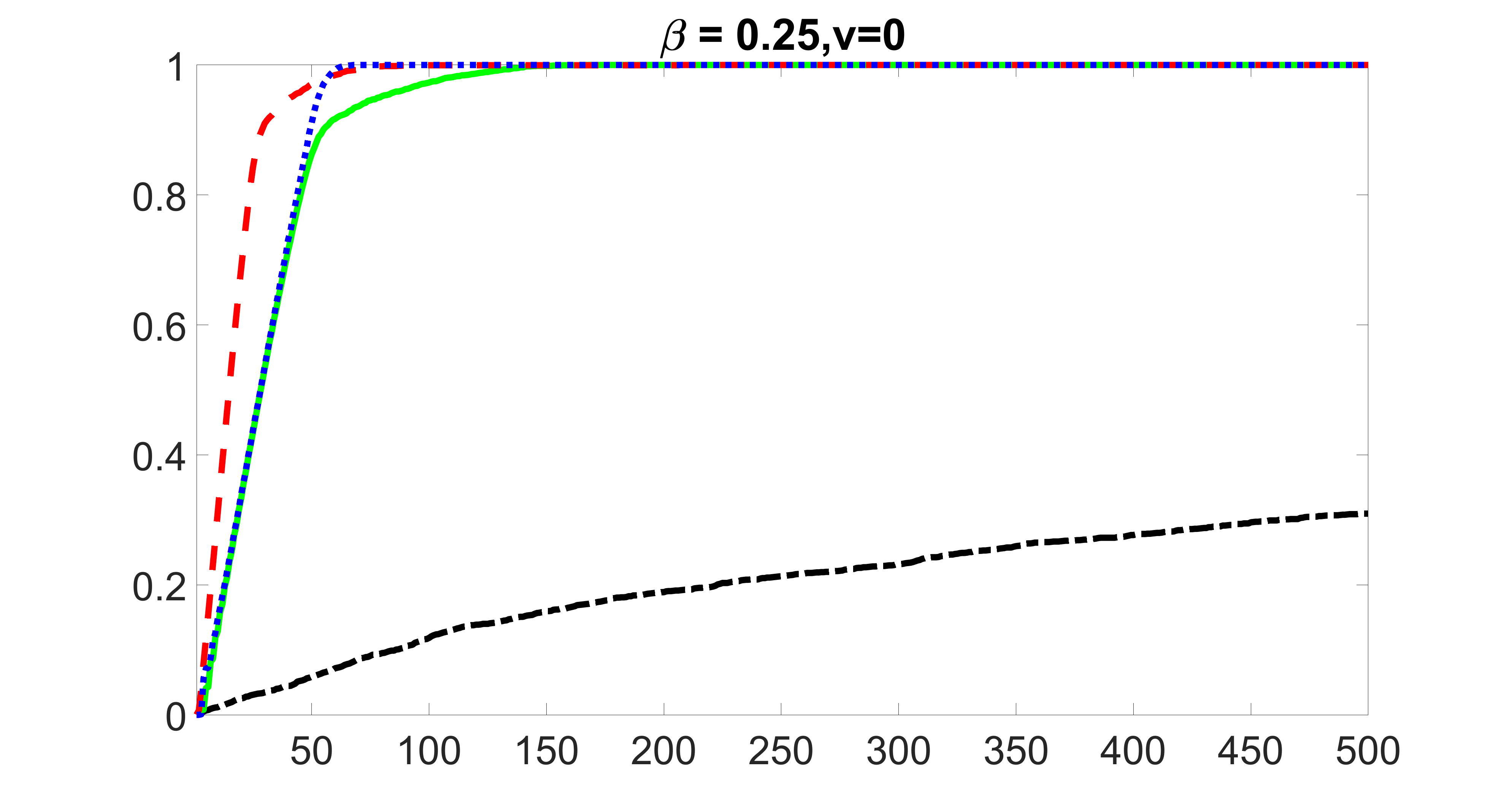
outcome, zero exposure
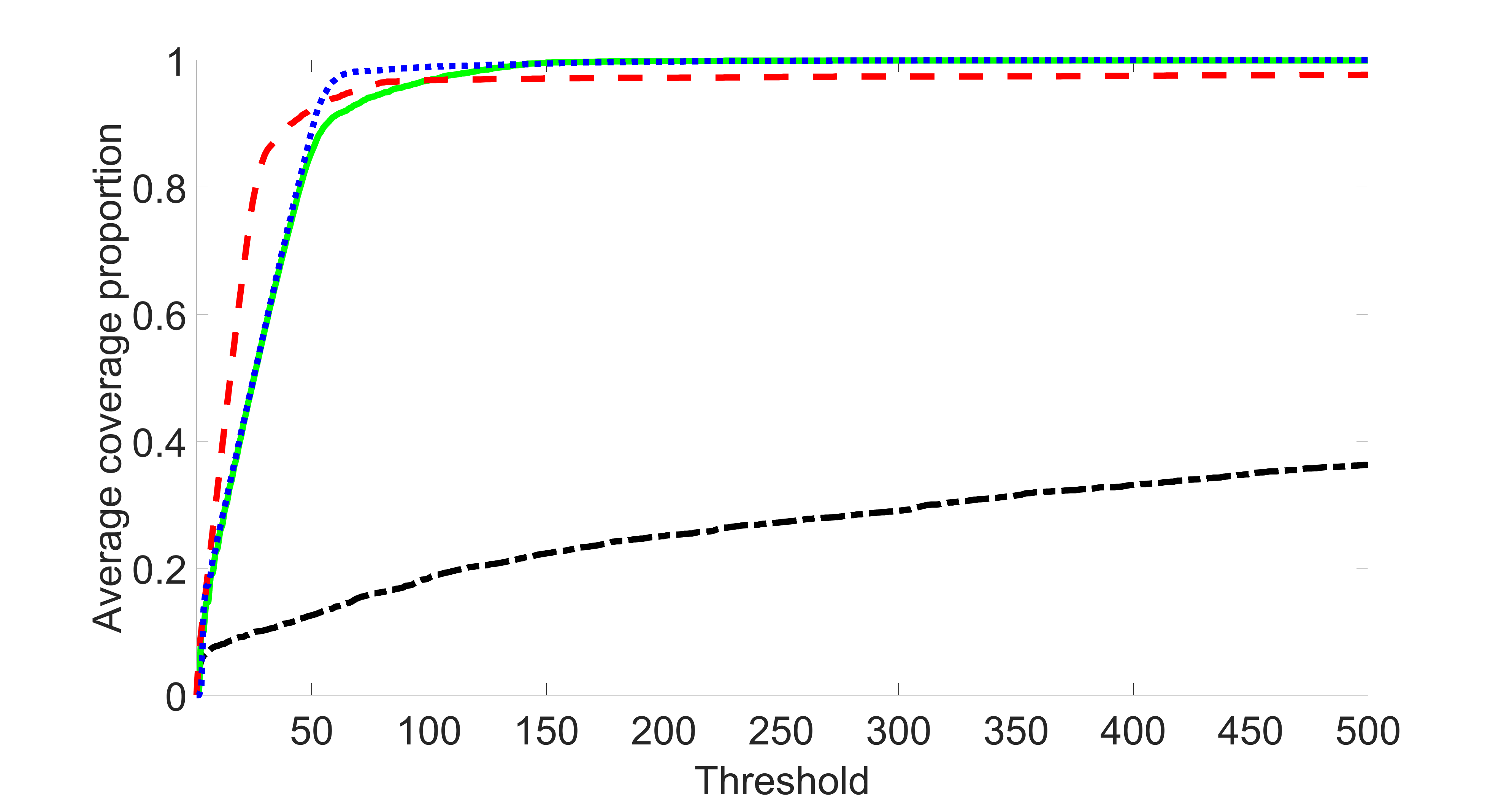
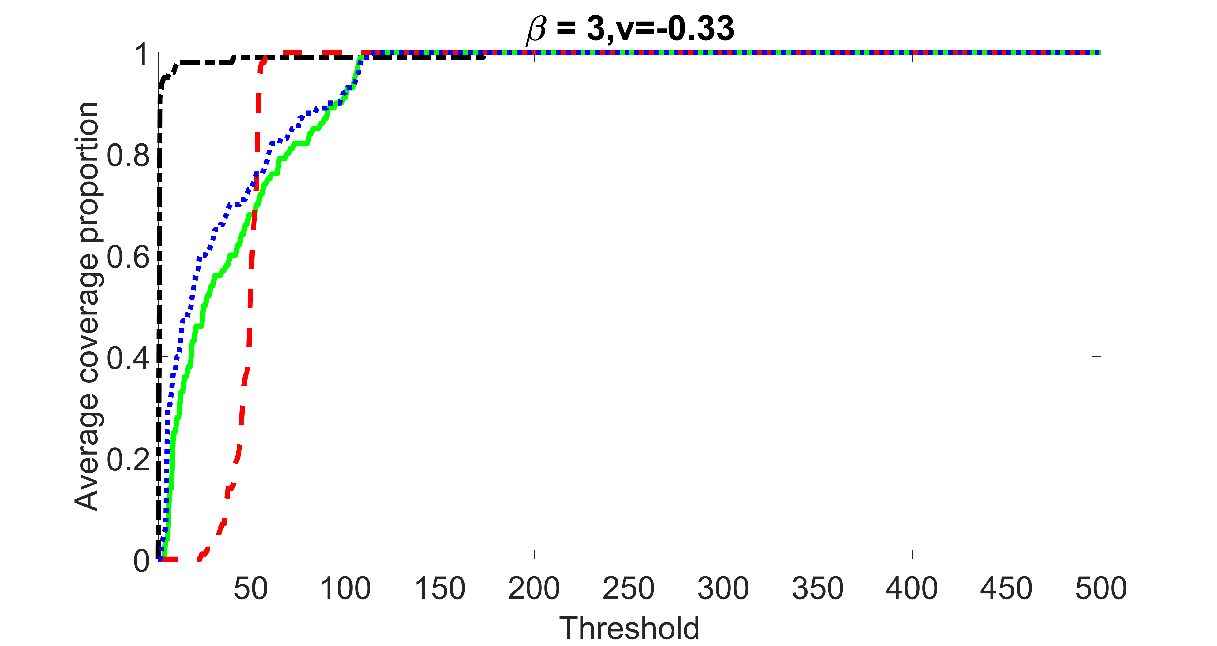
outcome, weak exposure
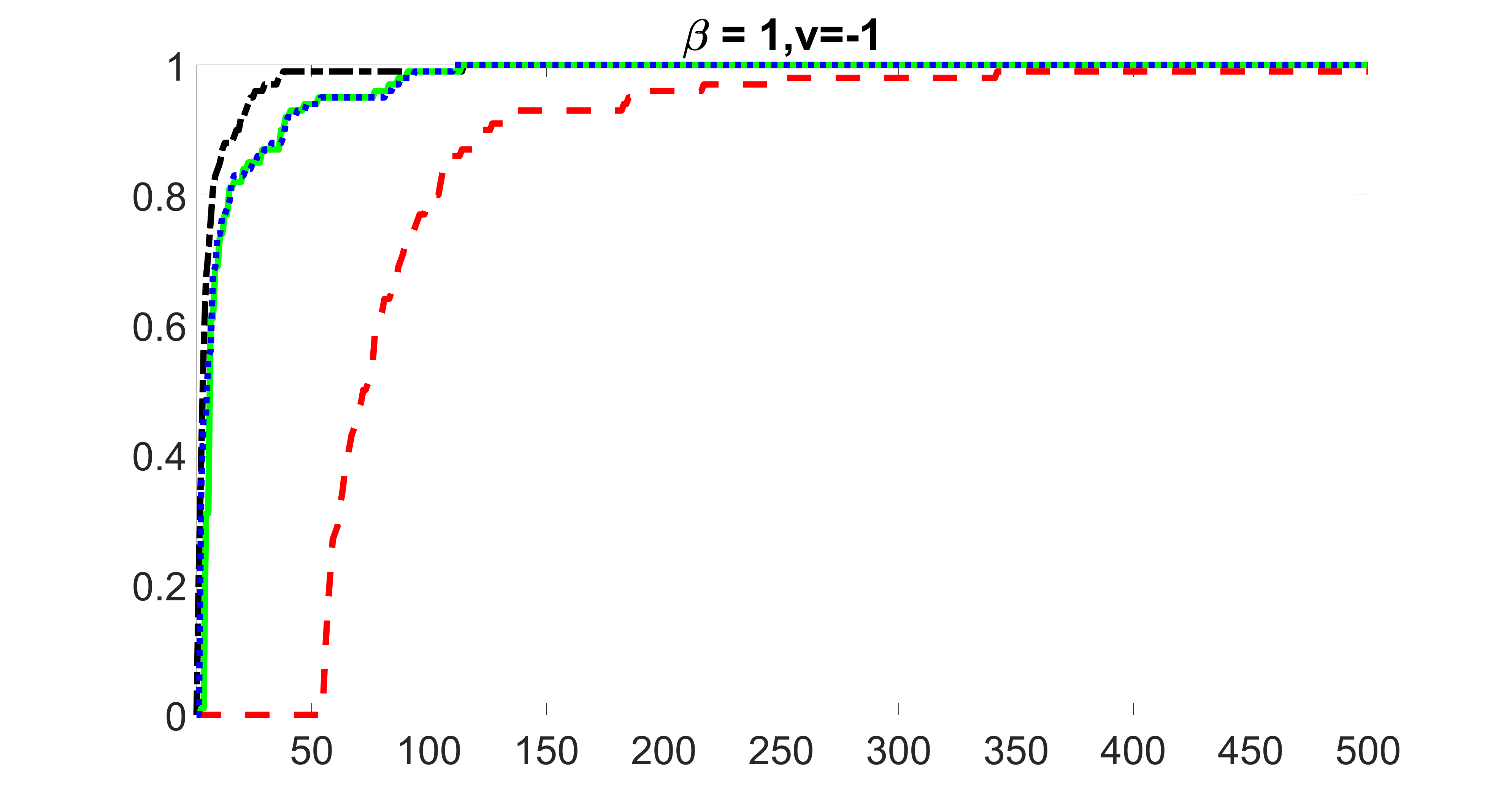
outcome, medium exposure
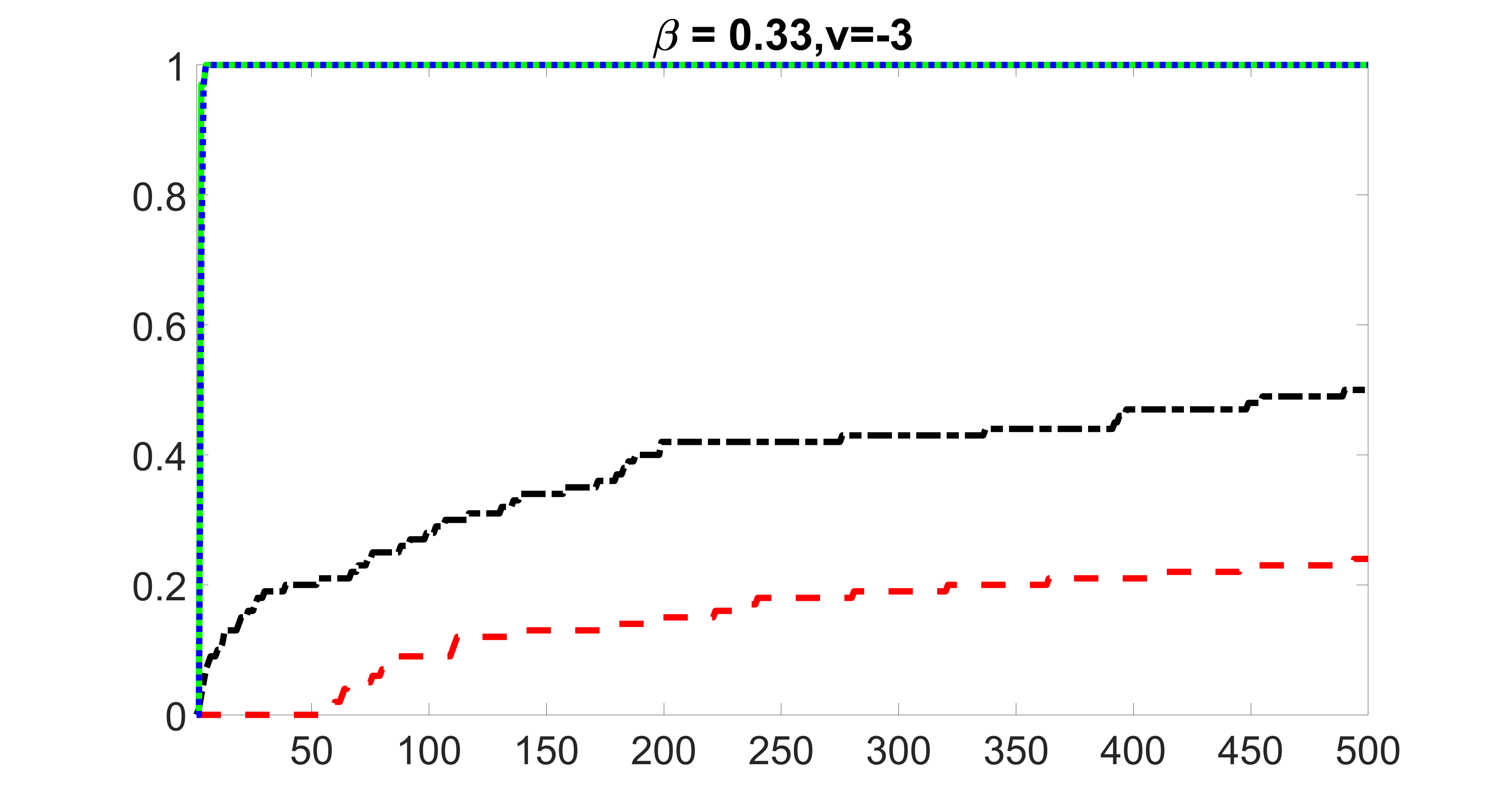
outcome, strong exposure
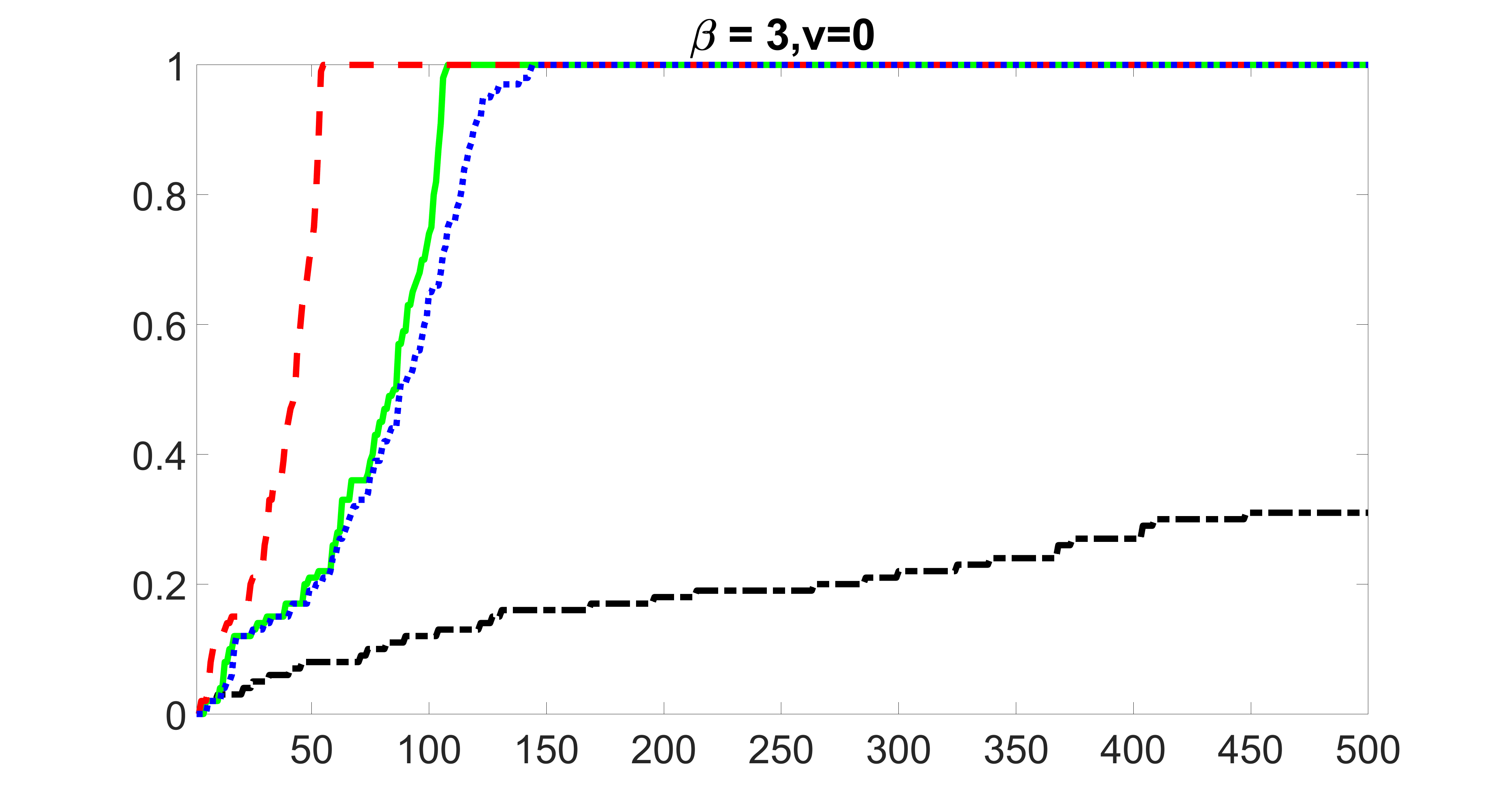
outcome, zero exposure
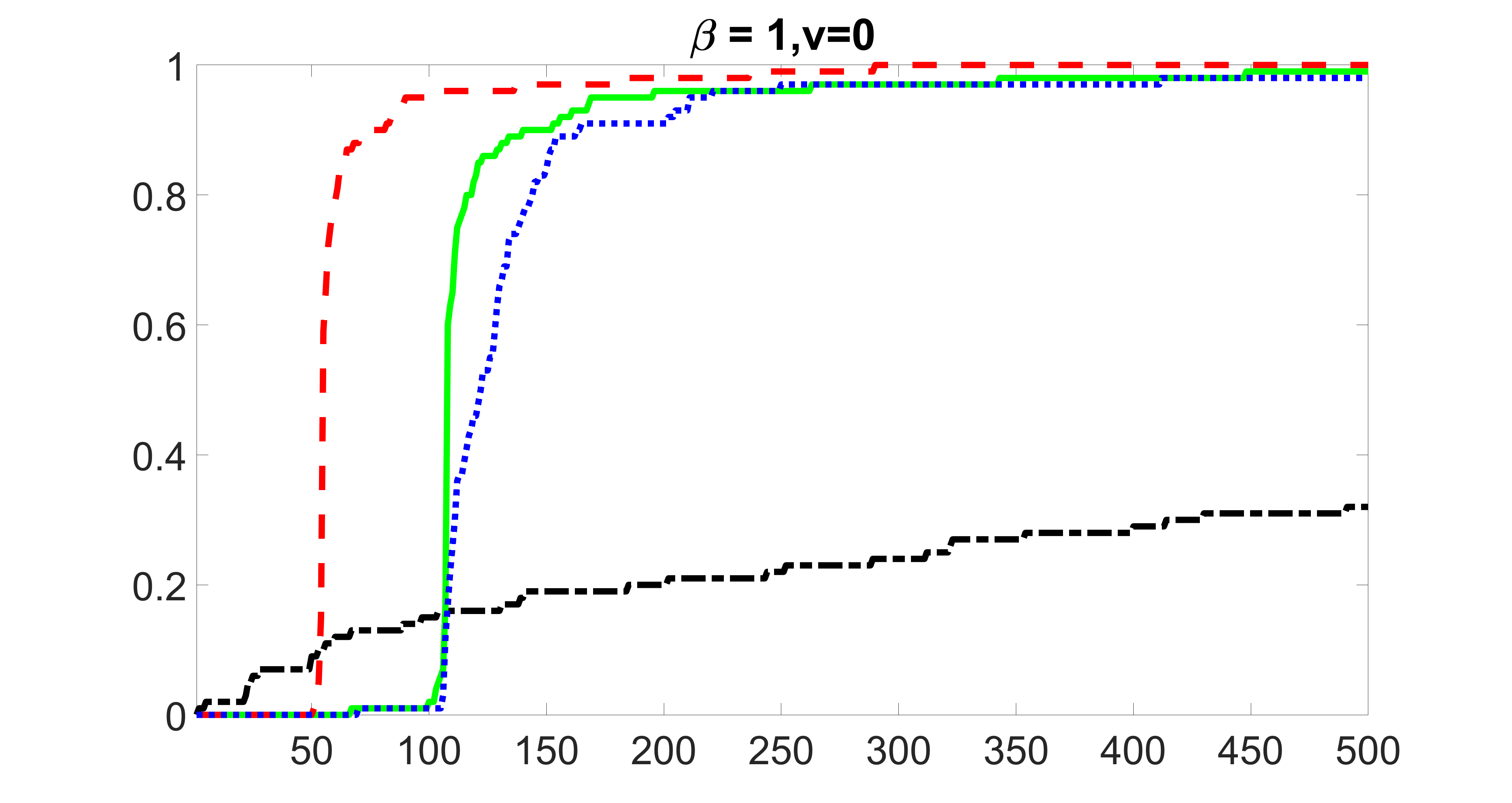
outcome, zero exposure
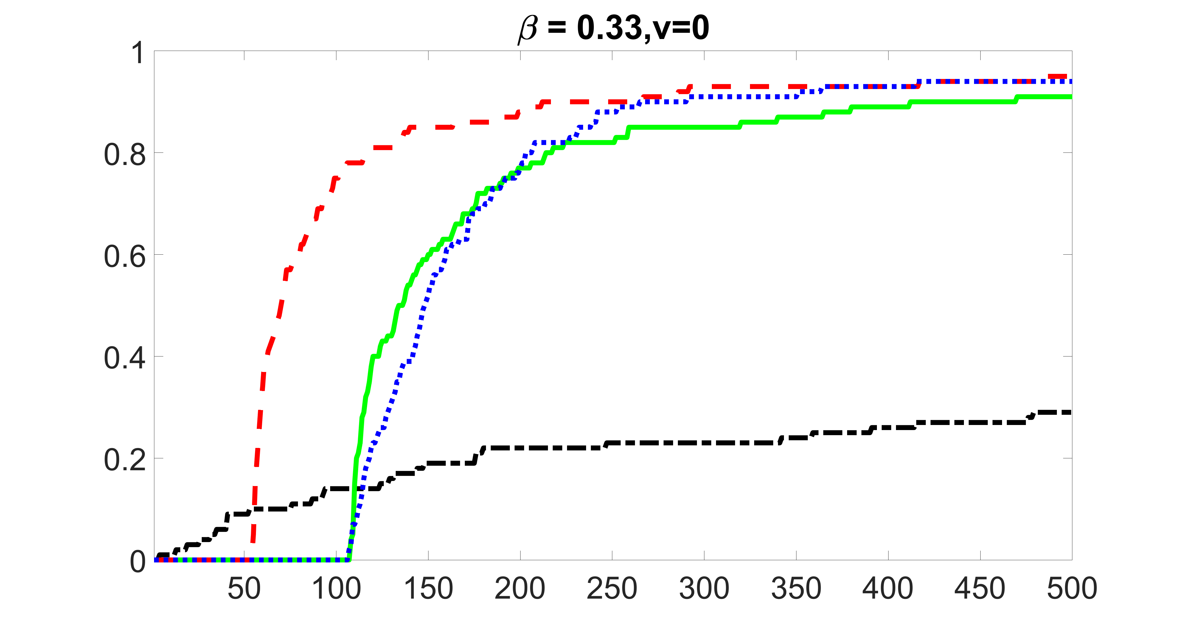
outcome, zero exposure
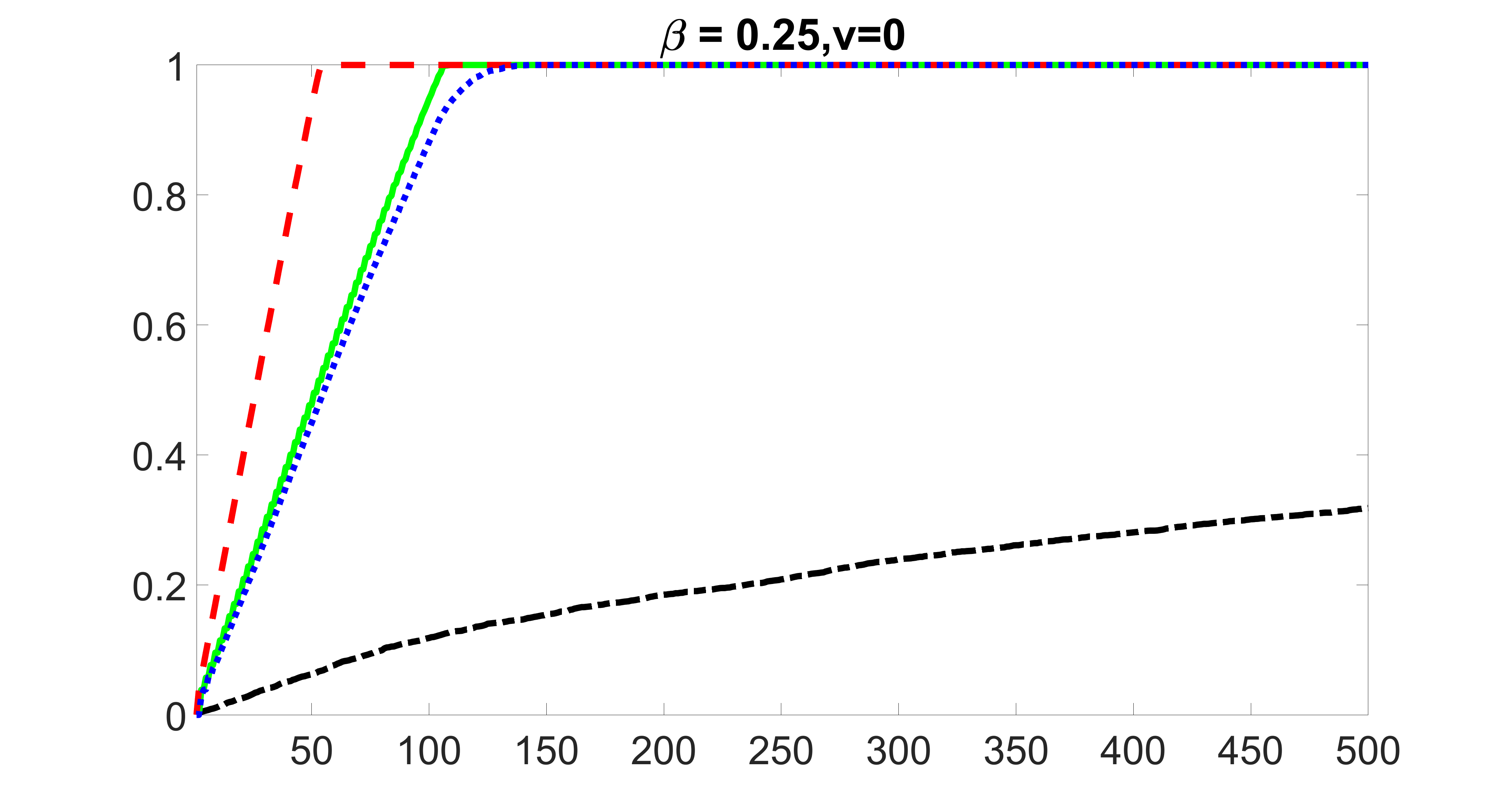
outcome, zero exposure
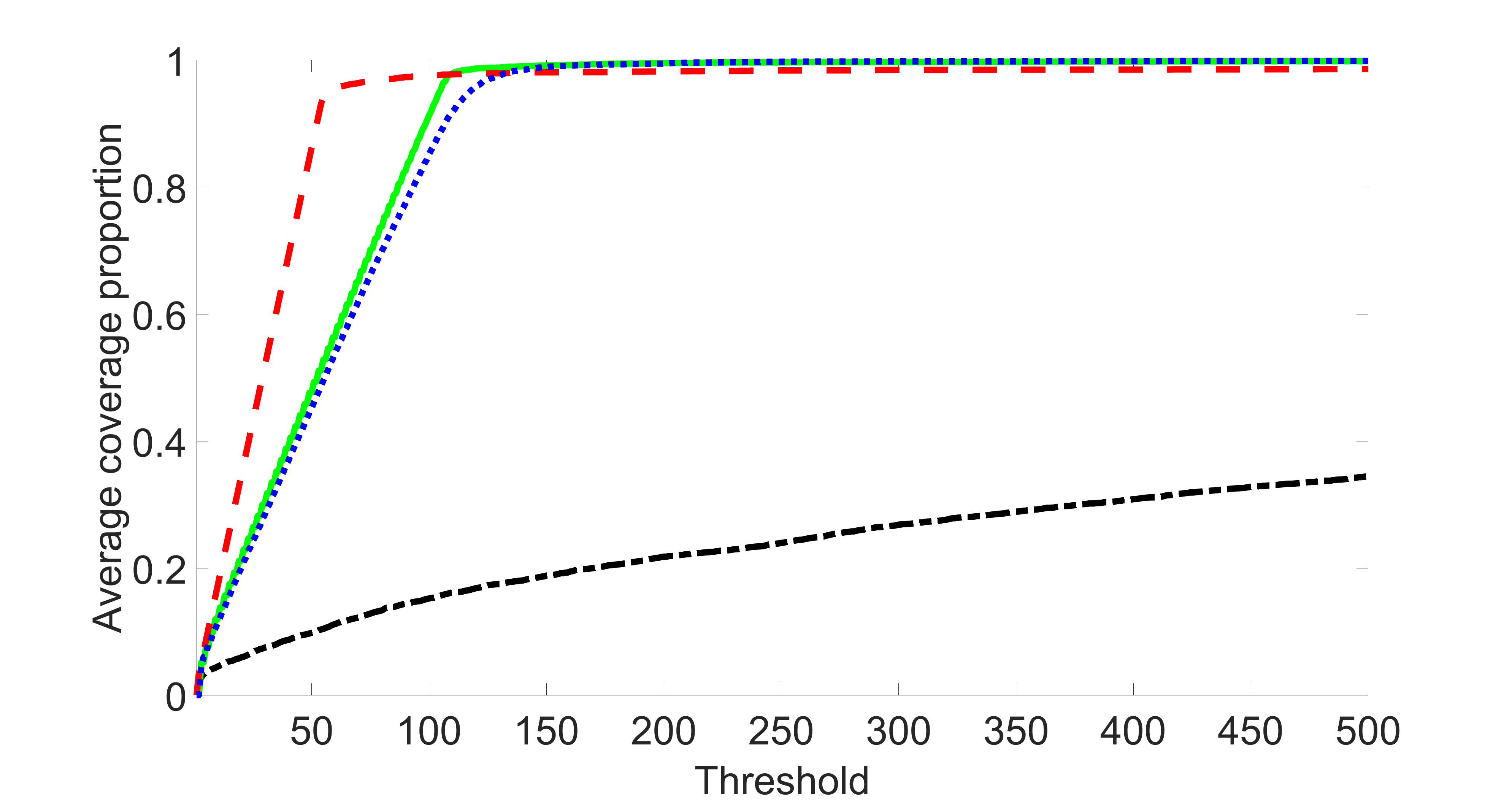
| Proposed | MSE | MSE | Proposed (block) | MSE | MSE |
|---|---|---|---|---|---|
| n=200,K=2 | 1.423(0.096) | 0.785(0.009) | n=200,K=2 | 1.390(0.090) | 0.793(0.010) |
| n=500,K=2 | 0.831(0.069) | 0.726(0.008) | n=500,K=2 | 0.892(0.082) | 0.734(0.009) |
| n=1000,K=2 | 0.591(0.050) | 0.676(0.008) | n=1000,K=2 | 0.488(0.028) | 0.666(0.006) |
| n=200,K=4 | 1.667(0.096) | 0.815(0.011) | n=200,K=4 | 1.548(0.088) | 0.805(0.010) |
| n=500,K=4 | 1.059(0.082) | 0.751(0.011) | n=500,K=4 | 1.094(0.090) | 0.758(0.012) |
| n=1000,K=4 | 0.606(0.057) | 0.671(0.008) | n=1000,K=4 | 0.555(0.045) | 0.678(0.008) |
| n=200,K=6 | 1.955(0.101) | 0.826(0.010) | n=200,K=6 | 1.701(0.084) | 0.816(0.009) |
| n=500,K=6 | 1.155(0.085) | 0.749(0.011) | n=500,K=6 | 1.107(0.089) | 0.752(0.011) |
| n=1000,K=6 | 0.578(0.051) | 0.674(0.008) | n=1000,K=6 | 0.551(0.047) | 0.672(0.008) |
| n=200,K=12 | 2.466(0.096) | 0.890(0.039) | n=200,K=12 | 2.223(0.129) | 0.838(0.011) |
| n=500,K=12 | 1.024(0.082) | 0.735(0.010) | n=500,K=12 | 0.927(0.077) | 0.727(0.008) |
| n=1000,K=12 | 0.570(0.046) | 0.673(0.008) | n=1000,K=12 | 0.627(0.057) | 0.681(0.009) |
| n=200,K=24 | 2.533(0.164) | 0.847(0.014) | n=200,K=24 | 2.136(0.138) | 0.821(0.010) |
| n=500,K=24 | 1.065(0.080) | 0.733(0.010) | n=500,K=24 | 1.119(0.088) | 0.737(0.011) |
| n=1000,K=24 | 0.662(0.050) | 0.669(0.008) | n=1000,K=24 | 0.677(0.056) | 0.673(0.009) |
| n=200,K=52 | 14.650(0.815) | 2.034(0.487) | n=200,K=52 | 13.693(0.728) | 1.870(0.459) |
| n=500,K=52 | 1.816(0.144) | 0.775(0.019) | n=500,K=52 | 1.725(0.143) | 0.762(0.019) |
| n=1000,K=52 | 0.937(0.066) | 0.684(0.010) | n=1000,K=52 | 0.861(0.056) | 0.675(0.008) |
15 Theoretical properties
Starting from here, we denote , and as the true values for , and respectively. Furthermore, we denote , , and as the true index sets of , , and .
15.1 Sure screening property
In this subsection, we study theoretical properties for our screening procedure. We let , where and . Here and are the true values for and , respectively, and is the true value of .
We have the following theorems, where the assumptions needed are included in Section 16.
Theorem 1.
Under Assumptions (A0) – (A3) and (A5), let and with , then we have as .
Since the screening procedure automatically includes all the significant covariates for small value of and , it is necessary to consider the size of , which we quantify in Theorem 2.
Theorem 2.
Under Assumptions (A0) – (A5), when and with , we have as .
Corollary 1.
Under Assumptions (A0) – (A5), when and with , we have as .
Theorem 1 shows that if and are chosen properly, our screening procedure will include all significant variables with a high probability. Theorem 2 guarantees that the size of selected model from the screening procedure is only of a polynomial order of even though the original model size is of an exponential order of . Therefore, the false selection rate of our screening procedure vanishes as , while the size of grows in a polynomial order of , where the order depends on two constants and defined in Section 16. Theorem 3 shows our blockwise screening procedure also enjoys the screening property. The proofs of these theorems are collected in Section 18.
Theorem 3.
Under Assumptions (A0) – (A3), (A5), and further assume the -th block size for some constant . Let , with , , and with , then we have as .
15.2 Theory for two-step estimator
In this section, we develop a unified theory for our two-step estimator. In particular, we derive a non-asymptotic bound for the final estimates. We first introduce some notation.
Denote parameter , where and . Using this notation, problem (3) can be recasted as minimizing , where , and . In addition, we let be the true value for , where and is the true values for and , respectively. Let be the proposed estimator for , where and are the estimators obtained from (3) for tuning parameters .
We hereby give nonasymptotic error bound for the proposed two-step estimator :
Theorem 4.
(Nonasymptotic error bounds for two-step estimator) Under Assumptions (A0) – (A9), and , and the condition that with , conditional on , there exists some positive constants , , , and , such that for and , with probability at least , one has
The bound in Theorem 4 implies that the convergence rate of the proposed estimator is . Here is a positive constant defined in Assumption (A6) in Section 16, and is the rank of . The convergence rate is controlled by and , where controls the exponential rates of model complexity that can diverge and controls the rate of largest eigenvalue of population covariance matrix that can grow. The proof of the theorem is deferred to section 18.
16 Assumptions for main theorems
In this section, we state the assumptions for the main theorems. We first make the following assumptions, which are needed for Theorems 1 and 2.
(A0) The covariates are independent and identically distributed (i.i.d) with mean zero and covariance . The random error are i.i.d with mean zero and variance . Define . The vectorized error matrices are i.i.d with mean zero and covariance . There exists a constant such that . Moreover, is independent of and .
(A1) There exist some constants and , and such that
and .
(A2) There exist positive constants and such that
for every , and .
Denote is a n-dimensional vector of zero-mean,
there exists a constant such that for any fixed ,
for all .
(A3) There exists a constant such that for .
(A4) There exists constants and such that .
(A5) .
Before we state the assumptions for Theorem 4, we first introduce some notations.
Denote where and . In addition, let , the true rank of matrix . Let us consider the class of matrices that have rank . For any given matrix , we let and denote its row and column space, respectively. Let and be a given pair of -dimensional subspace and , respectively.
For a given and pair , we define the subspace , , , , and as follows:
Denote with and . Then and ; and . We write with and let represent the -th column of for . With loss of generality we assume that has been column normalized, i.e. , for all .
We need the following assumptions:
(A6) Define
and assume that is a positive constant.
(A7) Assume and as with .
(A8) The vectorized error matrices are i.i.d. , where .
(A9) holds.
17 Auxiliary lemmas
In this section, we include the auxiliary lemmas needed for the theorems and their proofs.
Lemma 1.
(Bernstein’s inequality) Let be independent random variable with zero mean such that , for every (and all i) and some constant and . Then
for .
This is Lemma 2.2.11 from van der Vaart and Wellner (2000) and we omit the proof here.
Lemma 2.
Under Assumptions (A0), (A1) and (A2), for arbitrary and for every , we have that
Proof of Lemma 2:.
Note that the last part of Assumption (A2) actually implies that, there exist positive constants and , such that by applying Theorem 3.1 from Rivasplata (2012). Therefore, it can be unified into the first part of Assumption (A2) which implies that
for every , and . Therefore, by Assumptions (A0) and (A2) and Jensen’s inequality, we have
Then for every , one has
It follows from Lemma 1 that
Similarly we obtain
Then for every , one has
It follows from Lemma 1 that
Similarly we have
Then following the proof of showing second inequality, one has
∎
The following lemma is a standard result called Gaussian comparison inequality (Anderson, 1955).
Lemma 3.
Let and be zero-mean vector Gaussian random vectors with covariance matrix and respectively. If is positive semi-definite, then for any convex symmetric set , .
18 Proof of theorems
Proof of Theorem 1:.
We can write
Firstly, recall that i.e. . For every , and , we have
It follows from Assumptions (A0), (A1), (A2) and Lemma 2 that for any , one has
Therefore, for every , we have
Let
We have for every ,
| (5) |
Let us consider . recall that, , , and . For every , we have
It follows from Assumptions (A0), (A1), (A2) and Lemma 2 that for any , we have
Proof of Theorem 2.
The proof consists of two steps. In step 1, we will show that , where , and Recall that . Let and with , we have
By Assumptions (A3) and (A5), we have
for some constants and . Therefore, we have as .
In step 2, we will show that . As , we only need to show that both and are .
Define and . By the definition of , we have
Define and , we can write
Multiplying on both sides and taking expectations yield . Therefore, we have
By Assumption (A4), we have . This implies that .
Define . As , we have . By the definition of , we have
Define , we can write . Multiplying on both sides and taking expectations yield .
By Assumption (A4), we have .
Combining results from two steps above leads to . ∎
Proof of Theorem 3:.
We can write
Firstly, recall that i.e. . For every , and , we have
It follows from Assumptions (A0), (A1), (A2) and Lemma 2 that for any , one has
Therefore, for every , we have
Let
We have for every ,
| (7) |
Let us consider . recall that, , , and . For every , we have
It follows from Assumptions (A0), (A1), (A2) and Lemma 2 that for any , we have
Proof of Theorem 4:.
Denote , where and . In addition, for a given pair , we let be the true value for with and being true values for and respectively, and be the proposed estimator for with and being the estimators for and respectively. Furthermore, we let , the true rank of matrix . Let us consider the class of matrices that have rank . For any given matrix , we let and denote its row and column space, respectively. Let and be a given pair of -dimensional subspace and , respectively.
For a given and pair , we define the subspace , , , , and as followed:
where and are the orthogonal complements for and respectively. For simplicity, we will use , and to denote , and , respectively; and use , and to denote , and . It is easy to see that both and satisfy the condition that they are decomposable with respect to the subspace pair and , respectively. Therefore the regularizer terms and satisfies condition (G1) of Negahban et al. (2012).
Here we define the function by
where, with and . Next, We will derive a lower bound for .
Before we formally prove the result, we first introduce the concept of subspace compatibility constant. For a subspace , the subspace compatibility constant with respect to the pair is given by
Therefore, we have
where the last step of first inequality is obtained by applying Cauchy-Schwarz inequality. Furthermore, we have
where the first inequality follows from Assumption (A6) and the second inequality follows from Lemma 3 in Negahban et al. (2012). By the Cauchy-Schwarz inequality applied to and its dual , , where is defined as the dual norm of such that , we have If holds, where and (Negahban et al., 2012; Kong et al., 2020), one has Therefore, we have
By the subspace compatibility, we have , for . Substituting them into the previous inequality, and noticing that , we obtain that
The right hand side is a quadratic form of . Therefore, as long as , one has . Therefore, by Lemma 4 in Negahban et al. (2012), we can establish that
for some constant . It is easy to see that there exists some constant such that
Now we calculate and . According to Kong et al. (2020); Negahban et al. (2012), we have that and , where and .
We first calculate . Denoting , , where for . we let , where represent the -th column of . Since column normalized, i.e. , for all , by Assumption (A2), there exists a constant such that . Applying union bound, we have . By choosing , we can see that when , then there exist a positive constant such that the choice of holds with probability at least .
Secondly, we calculate :
Under condition (A1), . Therefore, we have
Therefore, by choosing , for any choice of , we guarantee that therefore is valid with probability at least for some positive constant .
On the other hand, let be a random matrix with each entry i.i.d. standard normal. By Assumption (A8) and Lemma 3, conditioning on we have
since .
As conditioning on , each entry of the matrix is i.i.d. . Since is a random variable with degrees of freedom, one has
using the tail bound of presented by the corollary of Lemma 1 from Laurent and Massart (2000). Combing with the standard random matrix theory, we know that with probability at least where and are some positive constants. Combining with what we got from previous step, we have holds with probability at least . Therefore, the choice of holds with probability at least .
As a result, the event that both and satisfy the above inequalities holds with probability at least for some postive constants , , and .
In sum, there exists some positive constants , with probability at least , one has
for some constants . This completes the proof.
∎
References
- Aizenstein et al. (2008) Aizenstein, H. J., R. D. Nebes, J. A. Saxton, J. C. Price, C. A. Mathis, N. D. Tsopelas, S. K. Ziolko, J. A. James, B. E. Snitz, P. R. Houck, et al. (2008). Frequent amyloid deposition without significant cognitive impairment among the elderly. Archives of Neurology 65(11), 1509–1517.
- Anderson (1955) Anderson, T. W. (1955). The integral of a symmetric unimodal function over a symmetric convex set and some probability inequalities. Proceedings of the American Mathematical Society 6(2), 170–176.
- Apostolova et al. (2006) Apostolova, L. G., I. D. Dinov, R. A. Dutton, K. M. Hayashi, A. W. Toga, J. L. Cummings, and P. M. Thompson (2006). 3D comparison of hippocampal atrophy in amnestic mild cognitive impairment and Alzheimer’s disease. Brain 129(11), 2867–2873.
- Apostolova et al. (2010) Apostolova, L. G., L. Mosconi, P. M. Thompson, A. E. Green, K. S. Hwang, A. Ramirez, R. Mistur, W. H. Tsui, and M. J. de Leon (2010). Subregional hippocampal atrophy predicts Alzheimer’s dementia in the cognitively normal. Neurobiology of Aging 31(7), 1077–1088.
- Barrett et al. (2005) Barrett, J. C., B. Fry, J. Maller, and M. J. Daly (2005). Haploview: analysis and visualization of LD and haplotype maps. Bioinformatics 21(2), 263–265.
- Barut et al. (2016) Barut, E., J. Fan, and A. Verhasselt (2016). Conditional sure independence screening. Journal of the American Statistical Association 111(515), 1266–1277.
- Beck and Teboulle (2009) Beck, A. and M. Teboulle (2009). A fast iterative shrinkage-thresholding algorithm for linear inverse problems. SIAM Journal on Imaging Sciences 2(1), 183–202.
- Bertram and Tanzi (2020) Bertram, L. and R. E. Tanzi (2020). Genomic mechanisms in Alzheimer’s disease. Brain Pathology 30(5), 966–977.
- Bi et al. (2017) Bi, X., L. Yang, T. Li, B. Wang, H. Zhu, and H. Zhang (2017). Genome-wide mediation analysis of psychiatric and cognitive traits through imaging phenotypes. Human Brain Mapping 38(8), 4088–4097.
- Blackstad et al. (1970) Blackstad, T., K. Brink, J. Hem, and B. June (1970). Distribution of hippocampal mossy fibers in the rat. An experimental study with silver impregnation methods. Journal of Comparative Neurology 138(4), 433–449.
- Braak and Braak (1998) Braak, H. and E. Braak (1998). Evolution of neuronal changes in the course of Alzheimer’s disease. In Ageing and Dementia, pp. 127–140. Springer.
- Brookhart et al. (2006) Brookhart, M. A., S. Schneeweiss, K. J. Rothman, R. J. Glynn, J. Avorn, and T. Stürmer (2006). Variable selection for propensity score models. American Journal of Epidemiology 163(12), 1149–1156.
- Cai et al. (2010) Cai, J.-F., E. J. Candès, and Z. Shen (2010). A singular value thresholding algorithm for matrix completion. SIAM Journal on Optimization 20(4), 1956–1982.
- Chung et al. (2014) Chung, S. J., M.-J. Kim, J. Kim, Y. J. Kim, S. You, J. Koh, S. Y. Kim, and J.-H. Lee (2014). Exome array study did not identify novel variants in Alzheimer’s disease. Neurobiology of Aging 35(8), 1958–e13.
- Consortium et al. (2012) Consortium, . G. P. et al. (2012). An integrated map of genetic variation from 1,092 human genomes. Nature 491, 56–65.
- Coon et al. (2007) Coon, K. D., A. J. Myers, D. W. Craig, J. A. Webster, J. V. Pearson, D. H. Lince, V. L. Zismann, T. G. Beach, D. Leung, L. Bryden, et al. (2007). A high-density whole-genome association study reveals that APOE is the major susceptibility gene for sporadic late-onset Alzheimer’s disease. The Journal of Clinical Psychiatry 68(4), 613–618.
- De Leon et al. (1989) De Leon, M., A. George, L. Stylopoulos, G. Smith, and D. Miller (1989). Early marker for Alzheimer’s disease: the atrophic hippocampus. The Lancet 334(8664), 672–673.
- Dehman et al. (2015) Dehman, A., C. Ambroise, and P. Neuvial (2015). Performance of a blockwise approach in variable selection using linkage disequilibrium information. BMC Bioinformatics 16(1), 1–14.
- Du et al. (2018) Du, L., K. Liu, X. Yao, S. L. Risacher, J. Han, L. Guo, A. J. Saykin, and L. Shen (2018). Fast multi-task SCCA learning with feature selection for multi-modal brain imaging genetics. In 2018 IEEE International Conference on Bioinformatics and Biomedicine (BIBM), pp. 356–361. IEEE.
- Dudek et al. (2016) Dudek, S. M., G. M. Alexander, and S. Farris (2016). Rediscovering area CA2: unique properties and functions. Nature Reviews Neuroscience 17(2), 89–102.
- Fan and Lv (2008) Fan, J. and J. Lv (2008). Sure independence screening for ultrahigh dimensional feature space. Journal of the Royal Statistical Society: Series B (Statistical Methodology) 70(5), 849–911.
- Ferrari et al. (2014) Ferrari, D. V., M. E Avila, M. A Medina, E. Pérez-Palma, B. I Bustos, M. A Alarcon, et al. (2014). Wnt/-catenin signaling in Alzheimer’s disease. CNS & Neurological Disorders-Drug Targets (Formerly Current Drug Targets-CNS & Neurological Disorders) 13(5), 745–754.
- Ferreira and Klein (2011) Ferreira, S. T. and W. L. Klein (2011). The A oligomer hypothesis for synapse failure and memory loss in Alzheimer’s disease. Neurobiology of Learning and Memory 96(4), 529–543.
- Fox et al. (1996) Fox, N., E. Warrington, P. Freeborough, P. Hartikainen, A. Kennedy, J. Stevens, and M. N. Rossor (1996). Presymptomatic hippocampal atrophy in Alzheimer’s disease: a longitudinal MRI study. Brain 119(6), 2001–2007.
- Frozza et al. (2018) Frozza, R. L., M. V. Lourenco, and F. G. De Felice (2018). Challenges for Alzheimer’s disease therapy: insights from novel mechanisms beyond memory defects. Frontiers in Neuroscience 12, 37.
- Gabriel et al. (2002) Gabriel, S. B., S. F. Schaffner, H. Nguyen, J. M. Moore, J. Roy, B. Blumenstiel, J. Higgins, M. DeFelice, A. Lochner, M. Faggart, et al. (2002). The structure of haplotype blocks in the human genome. Science 296(5576), 2225–2229.
- Gao et al. (2016) Gao, L., Z. Cui, L. Shen, and H.-F. Ji (2016). Shared genetic etiology between type 2 diabetes and Alzheimer’s disease identified by bioinformatics analysis. Journal of Alzheimer’s Disease 50(1), 13–17.
- Gaugler et al. (2019) Gaugler, J., B. James, T. Johnson, A. Marin, and J. Weuve (2019). 2019 Alzheimer’s disease facts and figures. Alzheimer’s & Dementia 15(3), 321–387.
- Guerreiro and Bras (2015) Guerreiro, R. and J. Bras (2015). The age factor in Alzheimer’s disease. Genome Medicine 7(1), 106.
- Guo et al. (2019) Guo, Y., W. Xu, J.-Q. Li, Y.-N. Ou, X.-N. Shen, Y.-Y. Huang, Q. Dong, L. Tan, and J.-T. Yu (2019). Genome-wide association study of hippocampal atrophy rate in non-demented elders. Aging (Albany NY) 11(22), 10468–10484.
- Hampel et al. (2018) Hampel, H., M.-M. Mesulam, A. C. Cuello, M. R. Farlow, E. Giacobini, G. T. Grossberg, A. S. Khachaturian, A. Vergallo, E. Cavedo, P. J. Snyder, et al. (2018). The cholinergic system in the pathophysiology and treatment of Alzheimer’s disease. Brain 141(7), 1917–1933.
- Hao and Zhang (2014) Hao, N. and H. H. Zhang (2014). Interaction screening for ultrahigh-dimensional data. Journal of the American Statistical Association 109(507), 1285–1301.
- Hao et al. (2017) Hao, X., C. Li, L. Du, X. Yao, J. Yan, S. L. Risacher, A. J. Saykin, L. Shen, and D. Zhang (2017). Mining outcome-relevant brain imaging genetic associations via three-way sparse canonical correlation analysis in Alzheimer’s disease. Scientific Reports 7(1), 1–12.
- Hastie et al. (2009) Hastie, T., R. Tibshirani, and J. Friedman (2009). The Elements of Statistical Learning: Data mining, Inference, and Prediction (Second ed.). Springer Series in Statistics. Springer, New York.
- Hesse et al. (2001) Hesse, C., L. Rosengren, N. Andreasen, P. Davidsson, H. Vanderstichele, E. Vanmechelen, and K. Blennow (2001). Transient increase in total tau but not phospho-tau in human cerebrospinal fluid after acute stroke. Neuroscience Letters 297(3), 187–190.
- Jack et al. (2000) Jack, C., R. C. Petersen, Y. Xu, P. O’brien, G. Smith, R. Ivnik, B. F. Boeve, E. G. Tangalos, and E. Kokmen (2000). Rates of hippocampal atrophy correlate with change in clinical status in aging and AD. Neurology 55(4), 484–490.
- Jack et al. (2003) Jack, C., M. Slomkowski, S. Gracon, T. Hoover, J. Felmlee, K. Stewart, Y. Xu, M. Shiung, P. O’Brien, R. Cha, et al. (2003). MRI as a biomarker of disease progression in a therapeutic trial of milameline for AD. Neurology 60(2), 253–260.
- Jack Jr et al. (2013) Jack Jr, C. R., D. S. Knopman, W. J. Jagust, R. C. Petersen, M. W. Weiner, P. S. Aisen, L. M. Shaw, P. Vemuri, H. J. Wiste, S. D. Weigand, et al. (2013). Tracking pathophysiological processes in Alzheimer’s disease: an updated hypothetical model of dynamic biomarkers. The Lancet Neurology 12(2), 207–216.
- Jack Jr et al. (2010) Jack Jr, C. R., D. S. Knopman, W. J. Jagust, L. M. Shaw, P. S. Aisen, M. W. Weiner, R. C. Petersen, and J. Q. Trojanowski (2010). Hypothetical model of dynamic biomarkers of the Alzheimer’s pathological cascade. The Lancet Neurology 9(1), 119–128.
- Khan et al. (2015) Khan, W., C. Aguilar, S. J. Kiddle, O. Doyle, M. Thambisetty, S. Muehlboeck, M. Sattlecker, S. Newhouse, S. Lovestone, R. Dobson, et al. (2015). A subset of cerebrospinal fluid proteins from a multi-analyte panel associated with brain atrophy, disease classification and prediction in Alzheimer’s disease. PLoS One 10(8), e0134368.
- Kim et al. (2009) Kim, J., J. M. Basak, and D. M. Holtzman (2009). The role of apolipoprotein E in Alzheimer’s disease. Neuron 63(3), 287–303.
- Kong et al. (2020) Kong, D., B. An, J. Zhang, and H. Zhu (2020). L2RM: Low-rank linear regression models for high-dimensional matrix responses. Journal of the American Statistical Association 115(529), 403–424.
- Laurent and Massart (2000) Laurent, B. and P. Massart (2000). Adaptive estimation of a quadratic functional by model selection. Annals of Statistics 28(5), 1302–1338.
- Li et al. (2007) Li, S., F. Shi, F. Pu, X. Li, T. Jiang, S. Xie, and Y. Wang (2007). Hippocampal shape analysis of Alzheimer disease based on machine learning methods. American Journal of Neuroradiology 28(7), 1339–1345.
- Lin et al. (2015) Lin, W., R. Feng, and H. Li (2015). Regularization methods for high-dimensional instrumental variables regression with an application to genetical genomics. Journal of the American Statistical Association 110(509), 270–288.
- Liu et al. (2013) Liu, E., M. Li, W. Wang, and Y. Li (2013). MaCH-Admix: Genotype imputation for admixed populations. Genetic Epidemiology 37, 25–37.
- Maass et al. (2018) Maass, A., S. N. Lockhart, T. M. Harrison, R. K. Bell, T. Mellinger, K. Swinnerton, S. L. Baker, G. D. Rabinovici, and W. J. Jagust (2018). Entorhinal tau pathology, episodic memory decline, and neurodegeneration in aging. Journal of Neuroscience 38(3), 530–543.
- Majdi et al. (2020) Majdi, A., S. Sadigh-Eteghad, S. R. Aghsan, F. Farajdokht, S. M. Vatandoust, A. Namvaran, and J. Mahmoudi (2020). Amyloid-, tau, and the cholinergic system in Alzheimer’s disease: Seeking direction in a tangle of clues. Reviews in the Neurosciences 31(4), 391–413.
- Mohs et al. (1997) Mohs, R. C., D. Knopman, R. C. Petersen, S. H. Ferris, C. Ernesto, M. Grundman, M. Sano, L. Bieliauskas, D. Geldmacher, C. Clark, et al. (1997). Development of cognitive instruments for use in clinical trials of antidementia drugs: additions to the Alzheimer’s disease assessment scale that broaden its scope. Alzheimer Disease and Associated Disorders 11(suppl 2), S13–21.
- Morishima-Kawashima and Ihara (2002) Morishima-Kawashima, M. and Y. Ihara (2002). Alzheimer’s disease: -Amyloid protein and tau. Journal of Neuroscience Research 70(3), 392–401.
- Negahban et al. (2012) Negahban, S. N., P. Ravikumar, M. J. Wainwright, B. Yu, et al. (2012). A unified framework for high-dimensional analysis of -estimators with decomposable regularizers. Statistical Science 27(4), 538–557.
- Nesterov (1998) Nesterov, Y. (1998). Introductory lectures on convex programming volume i: Basic course. Lecture Notes 3(4), 5.
- Nitsch et al. (1992) Nitsch, R. M., B. E. Slack, R. J. Wurtman, and J. H. Growdon (1992). Release of Alzheimer amyloid precursor derivatives stimulated by activation of muscarinic acetylcholine receptors. Science 258(5080), 304–307.
- Noble et al. (2012) Noble, K. G., S. M. Grieve, M. S. Korgaonkar, L. E. Engelhardt, E. Y. Griffith, L. M. Williams, and A. M. Brickman (2012). Hippocampal volume varies with educational attainment across the life-span. Frontiers in Human Neuroscience 6, 307.
- Paterson et al. (2014) Paterson, R., J. Bartlett, K. Blennow, N. Fox, L. Shaw, J. Trojanowski, H. Zetterberg, and J. Schott (2014). Cerebrospinal fluid markers including trefoil factor 3 are associated with neurodegeneration in amyloid-positive individuals. Translational Psychiatry 4(7), e419.
- Pedraza et al. (2004) Pedraza, O., D. Bowers, and R. Gilmore (2004). Asymmetry of the hippocampus and amygdala in MRI volumetric measurements of normal adults. Journal of the International Neuropsychological Society 10(5), 664–678.
- Purcell et al. (2007) Purcell, S., B. Neale, K. Todd-Brown, L. Thomas, M. A. Ferreira, D. Bender, J. Maller, P. Sklar, P. I. De Bakker, M. J. Daly, et al. (2007). PLINK: a tool set for whole-genome association and population-based linkage analyses. The American Journal of Human Genetics 81(3), 559–575.
- Remnestål et al. (2021) Remnestål, J., S. Bergström, J. Olofsson, E. Sjöstedt, M. Uhlén, K. Blennow, H. Zetterberg, A. Zettergren, S. Kern, I. Skoog, et al. (2021). Association of CSF proteins with tau and amyloid levels in asymptomatic 70-year-olds. Alzheimer’s Research & Therapy 13(1), 1–19.
- Richardson et al. (2018) Richardson, T. S., J. M. Robins, and L. Wang (2018). Discussion of “Data-driven confounder selection via Markov and Bayesian networks” by Häggström. Biometrics 74(2), 403–406.
- Rivasplata (2012) Rivasplata, O. (2012). Subgaussian random variables: an expository note. Internet publication, PDF.
- Sargolzaei et al. (2015) Sargolzaei, S., A. Sargolzaei, M. Cabrerizo, G. Chen, M. Goryawala, S. Noei, Q. Zhou, R. Duara, W. Barker, and M. Adjouadi (2015). A practical guideline for intracranial volume estimation in patients with Alzheimer’s disease. BMC Bioinformatics 16(7), 1–10.
- Schisterman et al. (2009) Schisterman, E. F., S. R. Cole, and R. W. Platt (2009). Overadjustment bias and unnecessary adjustment in epidemiologic studies. Epidemiology (Cambridge, Mass.) 20(4), 488.
- Selkoe and Hardy (2016) Selkoe, D. J. and J. Hardy (2016). The amyloid hypothesis of Alzheimer’s disease at 25 years. EMBO Molecular Medicine 8(6), 595–608.
- Shi et al. (2013) Shi, J., P. M. Thompson, B. Gutman, and Y. Wang (2013, Sep). Surface fluid registration of conformal representation: application to detect disease burden and genetic influence on hippocampus. NeuroImage 78, 111–134.
- Shortreed and Ertefaie (2017) Shortreed, S. M. and A. Ertefaie (2017). Outcome-adaptive lasso: variable selection for causal inference. Biometrics 73(4), 1111–1122.
- Sims et al. (2020) Sims, R., M. Hill, and J. Williams (2020). The multiplex model of the genetics of Alzheimer’s disease. Nature Neuroscience 23(3), 311–322.
- Takei et al. (2009) Takei, N., A. Miyashita, T. Tsukie, H. Arai, T. Asada, M. Imagawa, M. Shoji, S. Higuchi, K. Urakami, H. Kimura, et al. (2009). Genetic association study on in and around the APOE in late-onset Alzheimer’s disease in Japanese. Genomics 93(5), 441–448.
- Tang et al. (2021) Tang, D., D. Kong, W. Pan, and L. Wang (2021). Ultra-high dimensional variable selection for doubly robust causal inference. Biometrics (just-accepted).
- Thompson et al. (2004) Thompson, P. M., K. M. Hayashi, G. I. de Zubicaray, A. L. Janke, S. E. Rose, J. Semple, M. S. Hong, D. H. Herman, D. Gravano, D. M. Doddrell, et al. (2004). Mapping hippocampal and ventricular change in Alzheimer’s disease. NeuroImage 22(4), 1754–1766.
- Van de Pol et al. (2006) Van de Pol, L., A. Hensel, F. Barkhof, H. Gertz, P. Scheltens, and W. Van Der Flier (2006). Hippocampal atrophy in Alzheimer’s disease: age matters. Neurology 66(2), 236–238.
- van der Vaart and Wellner (2000) van der Vaart, A. W. and J. A. Wellner (2000). Weak convergence. Springer.
- Vina and Lloret (2010) Vina, J. and A. Lloret (2010). Why women have more Alzheimer’s disease than men: gender and mitochondrial toxicity of amyloid- peptide. Journal of Alzheimer’s Disease 20(s2), S527–S533.
- Wall and Pritchard (2003) Wall, J. D. and J. K. Pritchard (2003). Haplotype blocks and linkage disequilibrium in the human genome. Nature Reviews Genetics 4(8), 587–597.
- Wang et al. (2011) Wang, Y., Y. Song, P. Rajagopalan, T. An, K. Liu, Y.-Y. Chou, B. Gutman, A. W. Toga, P. M. Thompson, ADNI, et al. (2011). Surface-based TBM boosts power to detect disease effects on the brain: an N = 804 ADNI study. NeuroImage 56(4), 1993–2010.
- Watson (2019) Watson, S. (2019). Brain atrophy (cerebral atrophy). available at: www.healthline.com/health/brain-atrophy (Mar. 2019).
- Weiner et al. (2013) Weiner, M. W., D. P. Veitch, P. S. Aisen, L. A. Beckett, N. J. Cairns, R. C. Green, D. Harvey, C. R. Jack, W. Jagust, E. Liu, et al. (2013). The Alzheimer’s Disease Neuroimaging Initiative: A review of papers published since its inception. Alzheimer’s & Dementia 9(5), e111–e194.
- Zhang et al. (1990) Zhang, M., R. Katzman, D. Salmon, H. Jin, G. Cai, Z. Wang, G. Qu, I. Grant, E. Yu, P. Levy, et al. (1990). The prevalence of dementia and Alzheimer’s disease in Shanghai, China: impact of age, gender, and education. Annals of Neurology: Official Journal of the American Neurological Association and the Child Neurology Society 27(4), 428–437.
- Zhao et al. (2019) Zhao, B., T. Luo, T. Li, Y. Li, J. Zhang, Y. Shan, X. Wang, L. Yang, F. Zhou, Z. Zhu, et al. (2019). Genome-wide association analysis of 19,629 individuals identifies variants influencing regional brain volumes and refines their genetic co-architecture with cognitive and mental health traits. Nature Genetics 51(11), 1637–1644.
- Zhou et al. (2020) Zhou, F., H. Zhou, T. Li, and H. Zhu (2020). Analysis of secondary phenotypes in multi-group association studies. Biometrics 76(2), 606–618.
- Zhou and Li (2014) Zhou, H. and L. Li (2014). Regularized matrix regression. Journal of the Royal Statistical Society: Series B (Statistical Methodology) 76(2), 463–483.
- Zhou et al. (2018) Zhou, X., Y. Chen, K. Y. Mok, Q. Zhao, K. Chen, Y. Chen, et al. (2018). Identification of genetic risk factors in the Chinese population implicates a role of immune system in Alzheimer’s disease pathogenesis. Proceedings of the National Academy of Sciences 115(8), 1697–1706.