$\mathcal{PT}$ Symmetry and Renormalisation in Quantum Field Theory

Carl M Bender¹ Alexander Felski² S P Klevansky³ and Sarben Sarkar⁴ ¹Department of Physics, Washington University, St Louis, Missouri 63130, USA cmb@wustl.edu ²Institut für Theoretische Physik, Universität Heidelberg, 69120 Heidelberg, Germany felski@thphys.uni-heidelberg.de ³Institut für Theoretische Physik, Universität Heidelberg, 69120 Heidelberg, Germany spk@physik.uni-heidelberg.de ⁴Department of Physics, King’s College London, London WC2R 2LS, UK sarben.sarkar@kcl.ac.uk

Abstract

Quantum systems governed by non-Hermitian Hamiltonians with $\mathcal{PT}$ symmetry are special in having real energy eigenvalues bounded below and unitary time evolution. We argue that $\mathcal{PT}$ symmetry may also be important and present at the level of Hermitian quantum field theories because of the process of renormalisation. In some quantum field theories renormalisation leads to $\mathcal{PT}$ -symmetric effective Lagrangians. We show how $\mathcal{PT}$ symmetry may allow interpretations that evade ghosts and instabilities present in an interpretation of the theory within a Hermitian framework. From the study of examples $\mathcal{PT}$ -symmetric interpretation is naturally built into a path integral formulation of quantum field theory; there is no requirement to calculate explicitly the $\mathcal{PT}$ norm that occurs in Hamiltonian quantum theory. We discuss examples where $\mathcal{PT}$ -symmetric field theories emerge from Hermitian field theories due to effects of renormalization. We also consider the effects of renormalization on field theories that are non-Hermitian but $\mathcal{PT}$ -symmetric from the start.

1 Introduction

Non-Hermitian Hamiltonians govern systems that in general receive energy from and/or dissipate energy into their environment and so they are typically not in equilibrium. Their energy is not conserved and their energy levels are complex. However, in 1998 [1] non-Hermitian $\mathcal{PT}$ systems were shown to offer new possibilities for unitary time evolution in quantum mechanics. Since then there has been extensive research activity [2], particularly in material science and optics, which has implemented the ideas of $\mathcal{PT}$ -symmetric quantum mechanics.

$\mathcal{PT}$ -symmetric quantum mechanics can be considered to be a one-dimensional quantum field theory. To date there have been no clear examples of $\mathcal{PT}$ -symmetric quantum field theory in higher dimensions. We examine the possibility that $\mathcal{PT}$ symmetry may emerge when considering the effect of quantum fluctuations in a higher-dimensional field theory. We also examine the converse process where we consider the effect of quantum fluctuations on an initially $\mathcal{PT}$ -symmetric quantum field theory.

Using numerical techniques the work of Bender and Boettcher [1] showed that quantum-mechanical Hamiltonians of the form

H=\frac{1}{2}p^{2}+x^{2}\left(ix\right)^{\epsilon}

(1)

have a real positive spectrum. Using a correspondence between ordinary differential equations and integrable field theory models, Dorey et al. [3] provided an analytical proof of the result of Bender and Boettcher.

Mostafazadeh [4] considered the framework of pseudo-Hermiticity which contained $\mathcal{PT}$ symmetry as a special case. A Hamiltonian $H$ is pseudo-Hermitian if $H$ is not selfadjoint but

H^{\dagger}=\eta H\eta^{-1},

(2)

where $\eta$ is a positive-definite Hermitian operator. In terms of $\eta$ the Hilbert space of states has a positive-definite inner product given by

\left\langle\varphi,\eta\chi\right\rangle

(3)

where $\left\langle,\right\rangle$ is a conventional inner product on the Hilbert space of states for the Hermitian part of the Hamiltonian. There is not a universal expression for $\eta$ , which is difficult to calculate in general. This would seem to imply an impediment to calculating correlation functions in $\mathcal{PT}$ -symmetric field theories. Within the context of quantum mechanics, formulated in terms of functional integrals, Jones and Rivers [5] showed through examples that it was not necessary to calculate $\eta$ . Hence, we shall take the path-integral representation as the definition of a quantum field theory and, except for the Lee model, not consider $\eta$ explicitly. It is a convenient formulation for both perturbative and nonperturbative calculations.

We consider four examples of field theories to illustrate three different aspects of $\mathcal{PT}$ symmetry:

1.

the Lee model and the elimination of ghosts [6];
2.

the role of the top quark and the Higgs instability [7] in the standard model of particle physics [8];
3.

the new epsilon expansion for $\mathcal{PT}$ -symmetric scalar field theory [9, 10];
4.

the functional renormalisation group and the preservation of $\mathcal{PT}$ symmetry in the infrared after renormalisation [11].

2 Role of $\mathcal{PT}$ symmetry in the Lee model

Hermitian quantum field theory (QFT) has been studied for many decades both perturbatively and nonperturbatively. QFT is considered to be a viable and successful description of quantum electrodynamics, the weak, and the strong interactions. The use of dispersion relations in QFT, provides a way to bypass some of the limitations of perturbation theory and was developed decades ago (starting with the work of Lehmann, Symanzik, and Zimmerman [12, 13]). The theory of dispersion relations is based on one particularly important assumption: There exists an interpolating (i.e. a renormalised) field $\phi(x)$ , where $\phi(x)$ denotes an arbitrary field of the theory, such that we have the weak convergence relation

\lim_{t\to\pm\infty}\matrixelement{\alpha}{\phi(x)-\phi_{\rm out,\,in}(x)}{\beta}=0,

(4)

where $\ket{\alpha}$ and $\ket{\beta}$ are experimentally accessible states and $\phi_{\rm out}$ and $\phi_{\rm in}$ are free field operators associated with noninteracting particles. The Green’s functions in dispersion relations are assumed to have been made finite by some form of renormalisation (which need not be specified). In this framework it is possible, within the context of any specified polynomial field-theory Lagrangian, to establish coupled integral equations among 1-particle irreducible Green’s functions. For example, in a Yukawa theory of a pseudoscalar field interacting with fermions, 2-point functions are coupled with the 3-point (vertex) function. One conclusion is that such a theory may contain ghosts unless the vertex function vanishes as the momentum transfer tends to infinity [13]. So it is quite possible that a Hermitian quantum field theory may contain ghosts. The Lee model [14], which we discuss next, is just such an example where the vertex function and in particular coupling-constant renormalisation is related to such unusual behaviour. The role of $\mathcal{PT}$ symmetry is crucial in banishing the ghosts and making the field theory viable [6].

2.1 Lee model

The Lee model is very different from the Standard Model of particle physics but it has the advantage of being soluble and so provides a testing ground for new methods in field theory. Indeed, the model was devised as a field theory whose coupling-constant and wave-function renormalisation could be computed exactly in principle. One variant of the model contains fields for infinitely heavy spinless fermions, which have two internal states $V$ and $N$ , as well as a neutral scalar field $\theta$ . Antifermions are not in the theory and so there is no crossing symmetry. The permitted reaction channel is

V\rightleftharpoons N+\theta,

(5)

but the channel

N\rightleftharpoons V+\theta

(6)

is not allowed.

In momentum space the Hamiltonian of the Lee model (in a space of finite volume $\mathcal{V}$ ) is

H=H_{0}+H_{\rm int},

(7)

where

H_{0}=m_{V}\overline{\psi}_{V}{\psi}_{V}+m_{N}\overline{\psi}_{N}{\psi}_{N}+\sum_{\bf k}\omega_{\bf k}a^{{\dagger}}_{\bf k}a_{\bf k}

(8)

and

H_{\rm int}=\delta m_{V}\overline{\psi}_{V}{\psi}_{V}-g_{0}{\mathcal{V}}^{-\frac{1}{2}}\sum_{\bf k}\frac{u(\omega_{\bf k})}{{{(2\omega_{\bf k})}}^{\frac{1}{2}}}(\overline{\psi}_{V}{\psi}_{N}a_{\bf k}+\overline{\psi}_{N}{\psi}_{V}a^{{\dagger}}_{\bf k}).

(9)

$u(\omega_{\bf k})$ is a dimensional cut-off function which is chosen to tend to $0$ for large $\omega_{\bf k}$ where $\omega_{\bf k}=\sqrt{{\bf k}^{2}+\mu^{2}}$ . Standard commutation and anti-commutation rules are assumed:

	$\displaystyle\{\overline{\psi}_{V},{\psi}_{V}\}$	$\displaystyle=\{\overline{\psi}_{N},{\psi}_{N}\}=1$		(10)
	$\displaystyle\left[a_{\bf k},a^{{\dagger}}_{\bf k^{\prime}}\right]$	$\displaystyle=\delta_{\bf k,\bf k^{\prime}}.$		(11)

All other commutators and anticommutators vanish. Bare operators and coupling constant appear in $H$ . However $m_{V},\,m_{N},\,{\rm and},\,\mu$ are renormalised parameters and so are determined by experiment; $\delta m_{V}$ is the mass counterterm for the $V$ particle and is a function of $g_{0}$ . No further mass renormalisation is actually needed. The coupling $g_{0}$ in principle is determined from the scattering cross-section of $N$ and $\theta$ although there are interesting complications of non-Hermiticity if the coupling is not small.

However, let us for the moment persist in the view that $g_{0}$ is real and so $H$ is Hermitian. Let us choose as a basis for the Hilbert space states of the form

\ket{}=\ket{n_{V},n_{N},\{{n_{\bf{k}}}\}}.

(12)

From $H$ it is clear that there are two conserved quantities $B$ and $Q$ :

B=n_{V}+n_{N},\quad Q=-N_{\theta}+n_{N},

(13)

where $N_{\theta}=\sum_{\bf k}n_{\bf k}$ . Hence the Hilbert space is partitioned into an infinite number of independent sectors with fixed $B$ and $Q$ . Although this makes the model soluble, the analysis of sectors with large $B$ and $Q$ is complicated. Since our main point is to show how renormalisation can lead to a non-Hermitian Hamiltonian, we simplify our analysis further by considering (i) a nontrivial sector $B=1$ and $Q=0$ and (ii) modifying the model so that there is no $\bf k$ dependence. This simplified model is a quantum-mechanical one since the quantum fields in (8) and (9) are replaced by quantum operators. Hence, infinities that arise from summing over an infinite set of modes in quantum field theory are absent but some features of coupling-constant renormalisation persist. The resulting Hamiltonian is $\mathcal{H}={\cal{H}}_{0}+{\cal{H}}_{1}$ , where

{\cal{H}}_{0}={m_{V}}V^{{\dagger}}V+m_{N}N^{{\dagger}}N+\mu a^{{\dagger}}a

(14)

and

{\cal{H}}_{1}=g_{0}(V^{{\dagger}}Na+a^{{\dagger}}N^{{\dagger}}V)+\delta m_{V}V^{{\dagger}}V.

(15)

We will look at the 2-dimensional Hilbert space associated with this sector and consider the eigenstates, which we will denote by

	$\displaystyle\ket{V}$	$\displaystyle=c_{11}\ket{1,0,0}+c_{12}\ket{0,1,1},$		(16)
	$\displaystyle\ket{N\theta}$	$\displaystyle=c_{21}\ket{1,0,0}+c_{22}\ket{0,1,1},$		(17)

with eigenvalues $m_{V}$ and $E_{N\theta}$ . Let us denote $(m_{V}+\delta m_{V})$ by $m_{V_{0}}$ , the bare mass of $V$ . The eigenvalues can be shown to satisfy the equations

	$\displaystyle m_{V}=$	$\displaystyle\frac{1}{2}(m_{N}+m_{\theta}+m_{V_{0}}-\sqrt{M_{0}^{2}+4g_{0}^{2}}),$		(18)
	$\displaystyle E_{N\theta}=$	$\displaystyle\frac{1}{2}(m_{N}+m_{\theta}+m_{V_{0}}+\sqrt{M_{0}^{2}+4g_{0}^{2}}),$		(19)

where $M_{0}\equiv m_{N}+m_{\theta}-m_{V_{0}}.$ Following field theory, we define the wave-function renormalisation constant $Z_{V}$ through the relation

1=\bra{0}\frac{1}{\sqrt{Z_{V}}}V\ket{V},

(20)

which gives

Z_{V}=\frac{2g_{0}^{2}}{\sqrt{M_{0}^{2}+4g_{0}^{2}}\,(\sqrt{M_{0}^{2}+4g_{0}^{2}}-M_{0})},

(21)

and the coupling constant renormalisation through

\frac{g^{2}}{g_{0}^{2}}=Z_{V}.

(22)

We deduce that

g_{0}^{2}=\frac{g^{2}}{1-\frac{g^{2}}{M^{2}}},

(23)

where $M\equiv m_{N}+m_{\theta}-m_{V}$ . If $g$ , the experimentally determined value, exceeds $M$ then $g_{0}$ becomes pure imaginary and the Hamiltonian becomes non-Hermitian. Although the Hamiltonian has become non-Hermitian, it is $\mathcal{PT}$ -symmetric. Explicitly, the transformations due to $\mathcal{P}$ are [6]

	$\displaystyle\mathcal{P}V\mathcal{P}$	$\displaystyle=-V,$	$\displaystyle\mathcal{P}N\mathcal{P}$	$\displaystyle=-N,$	$\displaystyle\mathcal{P}a\mathcal{P}$	$\displaystyle=-a,$		(24)
	$\displaystyle\mathcal{P}V^{{\dagger}}\mathcal{P}$	$\displaystyle=-V^{{\dagger}},$	$\displaystyle\mathcal{P}N^{{\dagger}}\mathcal{P}$	$\displaystyle=-N^{{\dagger}},$	$\displaystyle\mathcal{P}a^{{\dagger}}\mathcal{P}$	$\displaystyle=-a^{{\dagger}}.$		(25)

The transformations due to $\mathcal{T}$ are

	$\displaystyle\mathcal{T}V\mathcal{T}$	$\displaystyle=V,$	$\displaystyle\mathcal{T}N\mathcal{T}$	$\displaystyle=N,$	$\displaystyle\mathcal{T}a\mathcal{T}$	$\displaystyle=a$		(26)
	$\displaystyle\mathcal{T}V^{{\dagger}}\mathcal{T}$	$\displaystyle=V^{{\dagger}}$	$\displaystyle\mathcal{T}N^{{\dagger}}\mathcal{T}$	$\displaystyle=N^{{\dagger}}$	$\displaystyle\mathcal{T}a^{{\dagger}}\mathcal{T}$	$\displaystyle=a^{{\dagger}}.$		(27)

It is now straightforward to check that $i|g_{0}|(V^{{\dagger}}Na+a^{{\dagger}}N^{{\dagger}}V)$ is $\mathcal{PT}$ -symmetric. This is our first example of a $\mathcal{PT}$ -symmetric field theory that arises from a Hermitian field theory after renormalisation. On introducing a $\mathcal{PT}$ -symmetric inner product in the ghost regime of the Lee model, the so-called ghost state (identified within the Hermitian frame work) turns out to have a positive norm[6]. The Lee model then can be interpreted as an acceptable quantum field theory.

3 Higgs instability and $\mathcal{PT}$ symmetry

The conventional approach to renormalisation involves the regularisation of loop integrals in Feynman diagrams. This led to scale dependence of the parameters of the theory which can be understood in a different way using the approach [15] of Wilson to renormalisation. Wilson’s approach leads naturally to the concept of effective actions, and the form of the effective actions for some theories in high-energy physics is non-Hermitian and $\mathcal{PT}$ -symmetric.

The change from the conventional to the Wilson approach can be illustrated by considering a scalar field $\Phi$ whose (conventional) action is given by

S_{\Lambda}\left[\Phi\right]=\int d^{D}x(\frac{1}{2}\partial_{\mu}\Phi\partial^{\mu}\Phi+U_{\Lambda}(\Phi))

(28)

where the UV cut-off is $\Lambda$ . If we integrate over Fourier modes with momenta of magnitude $p$ in the shell $k\leq p\leq\Lambda$ we arrive at an action which we will denote by $S_{k}\left[\phi\right]$ where $\phi$ has Fourier modes with $p\leq k$ (a sharp infrared cut-off).¹¹1Wetterich [16] introduced a smooth infrared cut-off function $R_{k}(p^{2})$ rather than a sharp cut-off so that $S_{k}\left[\phi\right]=\int d^{D}x[\frac{1}{2}\partial_{\mu}\phi\partial^{\mu}+V_{k}(\phi)]+\Delta_{k}[\phi]$ , where $\Delta_{k}[\phi]=\frac{1}{2}\int d^{D}p\phi_{p}R_{k}(p^{2})\phi_{-p}$ . A common choice for $R_{k}(p^{2})$ is $R_{k}(p^{2})=(k^{2}-p^{2})\Theta(k^{2}-p^{2})$ . The associated partition function is

Z_{k}[j]\equiv\exp(-W_{k}[j])\equiv\int D\phi\exp(-S_{k}[\phi]-\int_{p}j_{p}\phi_{-p})

(29)

and a Legendre transformation on $W_{k}[j]$ leads to the effective action $\Gamma_{k}[\phi_{c}]$

\Gamma_{k}[\phi_{c}]=W_{k}\left[j\right]-\int d^{D}xj\phi_{c}-\Delta_{k}[\phi_{c}].

(30)

Within systematic (derivative) approximation schemes [16, 17] the effective action can be represented (at the lowest level of approximation) by the ansatz

\Gamma_{k}[\phi_{c}]=\int d^{D}x(\frac{1}{2}\partial_{\mu}\phi_{c}\partial^{\mu}\phi_{c}+U_{k}(\phi_{c})).

(31)

The effective potential, $U_{k}(\phi_{c})$ which results from renormalisation, will show the emergence of $\mathcal{PT}$ symmetry in the next models that we will discuss. This ansatz represents quite a severe approximation since, for an $x$ -independent $\phi_{c}$ , we have a one-dimensional approximation to an infinite-dimensional field.

We consider two theories of current interest using this formalism:

1.

a theory of dynamical breaking of gravity via a graviton condensate field [18] $\varphi_{c}$ with $U(\varphi_{c})=-{\varphi_{c}}^{4}\log(i\varphi_{c})$ for large $\varphi_{c}$ r,

and
2.

the Standard Model of particle physics for which $\varphi_{c}$ is the Higgs field and $U(\varphi_{c})=-{\varphi_{c}}^{4}\log(\varphi_{c}^{2})$ for large $\varphi_{c}$ [7].

Both examples, in conventional quantum mechanics, would show unstable behaviour for large $\varphi_{c}$ . Under $\mathcal{P}$ we have $\varphi_{c}\rightarrow{-\varphi_{c}}$ and under $\mathcal{T}$ we have $i\rightarrow{-i}$ . So $U(\varphi_{c})$ is $\mathcal{PT}$ symmetric in both cases.

We study such effective potentials by considering three related quantum mechanical Hamiltonians $H_{i}$ , $i=1,2,3$ :

$\displaystyle H_{1}=$	$\displaystyle p^{2}+{x^{4}}\log(ix),$	(32)
$\displaystyle H_{2}=$	$\displaystyle p^{2}-{x^{4}}\log(ix),$	(33)
$\displaystyle H_{3}=$	$\displaystyle p^{2}-x^{4}\log(x^{2}),$	(34)

which are non-Hermitian but $\mathcal{PT}$ -symmetric. We will find that the the first two Hamiltonians will show unbroken $\mathcal{PT}$ symmetry and the Hamiltonian $H_{3}$ will show broken $\mathcal{PT}$ symmetry.

3.1 The spectra for $H_{1}$

We use the WKB method of semiclassical quantum mechanics to determine the energy spectrum of $H_{1}$ :

•

Locate turning points.
•

Examine the complex classical trajectories on an infinite-sheeted Riemann surface.
•

Determine the open or closed nature of the trajectories.

The turning points satisfy the equation

E=x^{4}\log(ix).

(35)

We take $E=1.24909$ because this is the numerical value of the ground-state energy obtained separately by solving the Schrödinger equation. (See the table below.)

One turning point lies on the negative imaginary- $x$ axis. To find this point we set $x=-ir$ ( $r>0$ ) and obtain the algebraic equation $E=r^{4}\log r$ . Solving this equation by using Newton’s method, we find that the turning point lies at $x=-1.39316i$ . To find the other turning points we seek solutions to (35) in polar form $x=re^{i\theta}$ ( $r>0,\,\theta\,{\rm real}$ ). Substituting for $x$ in (35) and taking the imaginary part, we obtain

\log r=-(2k\pi+\theta+\pi/2)\cos(4\theta)/\sin(4\theta),

(36)

where $k$ is the sheet number in the Riemann surface of the logarithm. (We choose the branch cut to lie on the positive-imaginary axis.) Using (36), we simplify the real part of (35) to

E=-r^{4}(2k\pi+\theta+\pi/2)/\sin(4\theta).

(37)

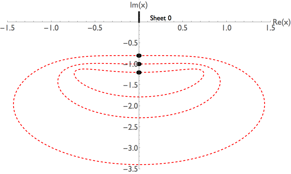
We then use (36) to eliminate $r$ from (37) and use Newton’s method to determine $\theta$ . For $k=0$ and $E=1.24909$ , two $\mathcal{PT}$ -symmetric (left-right symmetric) pairs of turning points lie at $\pm 0.93803-0.38530i$ and at $\pm 0.32807+0.75353i$ . For $k=1$ and $E=1.24909$ there is a turning point at $-0.53838+0.23100i$ ; the $\mathcal{PT}$ -symmetric image of this turning point lies on sheet $k=-1$ at $0.53838+0.23100i$ .

The turning points determine the shape of the classical trajectories. Two topologically different kinds of classical paths are shown in Figs. 1 and 2. All classical trajectories are closed and left-right symmetric, and this implies that the quantum energies are all real [19].

The WKB quantization condition is a complex path integral on the principal sheet of the logarithm ( $k=0$ ). On this sheet a branch cut runs from the origin to $+i\infty$ on the imaginary axis; this choice of branch cut respects the $\mathcal{PT}$ symmetry of the configuration. The integration path goes from the left turning point $x_{{\rm L}}$ to the right turning point $x_{{\rm R}}$ [20]:

\left(n+\frac{1}{2}\right)\pi\sim\int_{x_{{\rm L}}}^{x_{{\rm R}}}dx\sqrt{E-V(x)}\quad(n>>1).

(38)

Refer to caption — Figure 1: Three nested closed classical paths.

If the energy is large $\left(E_{n}\gg 1\right)$ , then from (36) with $k=0$ we find that the turning points lie slightly below the real axis at $x_{\rm R}=re^{i\theta}$ and at $x_{{\rm L}}=re^{-\pi i-i\theta}$ with

\theta\sim-\pi/(8\log r)\quad{\rm and}\quad r^{4}\log r\sim E.

(39)

We choose the path of integration in (38) to have a constant imaginary part so that the path is a horizontal line from $x_{{\rm L}}$ to $x_{{\rm R}}$ . Since $E$ is large, $r$ is large and thus $\theta$ is small. We obtain the simplified approximate quantization condition

\left(n+\frac{1}{2}\right)\pi\sim r^{3}\log r\int_{-1}^{1}dt\sqrt{1-t^{4}},

(40)

which leads to the WKB approximation for $n\gg 1$ :

\frac{E_{n}}{[\log(E_{n})]^{1/3}}\sim\left[\frac{\Gamma(7/4)(n+1/2)\sqrt{\pi}}{\Gamma(5/4)\sqrt{2}}\right]^{4/3}.

(41)

Calculation of values of energy
Energy level $n$	$E_{n}$	$\frac{E_{n}}{[\log(E_{n})]^{1/3}}$	WKB	% error
0	1.24909	2.06161	0.54627	73.5028
3	13.7383	9.96525	7.31480	26.5969
6	31.6658	20.9458	16.6979	20.2804
9	52.9939	33.4674	27.6956	17.2463
12	76.9748	47.1776	39.9324	15.3573

Analysis of the supergravity model Hamiltonian $H_{2}$ : The classical trajectories for the Hamiltonian $H_{2}$ are plotted in Figs. 3 and 4. Like the classical trajectories for the Hamiltonian $H_{1}$ ), these trajectories are closed, which implies that all the eigenvalues for $H_{2}$ are real.

Analysis of the Higgs model Hamiltonian $H_{3}$ : To make sense of $H_{3}$ we again introduce a parameter $\epsilon$ and we define $H_{3}$ as the limit of $H=p^{2}+x^{2}(ix)^{\epsilon}\log\left(x^{2}\right)$ as $\epsilon:\,0\to 2$ . This case is distinctly different from that for $H_{2}$ . Figure 5 shows that the $\mathcal{PT}$ symmetry is broken for all $\epsilon\neq 0$ . When $\epsilon=2$ , there are only four real eigenvalues: $E_{0}=1.1054311$ , $E_{1}=4.577736$ , $E_{2}=10.318036$ , and $E_{3}=16.06707$ . To confirm this result we plot a classical trajectory for $\epsilon=2$ in Fig. 6. In contrast with Fig. 4, the trajectory is open and not left-right symmetric.

4 Renormalisation and canonical scalar field theory

We have shown examples of $\mathcal{PT}$ -symmetric quantum field theories arising from the process of renormalisation in field theories. The properties of $\mathcal{PT}$ -symmetric field theories have yet to be established. In quantum mechanics much progress in understanding $\mathcal{PT}$ symmetry has been made through the study of the Hamiltonian in (1). A natural generalisation to an Euclidean field theory Hamiltonian in $D$ -dimensions is to consider the Lagrangian

L=\frac{1}{2}(\nabla\phi)^{2}+\frac{1}{2}\mu^{2}\varphi^{2}+\frac{1}{2}g\mu_{0}^{2}\phi^{2}(i\mu_{0}^{\frac{\delta}{2}}\phi)^{\epsilon}

(42)

where $\phi$ is a dimensional pseudoscalar field, $\delta=2-D$ and $\epsilon\geq 0$ . It is natural to study this class of field theories since we can then compare our findings in certain limits with those found in quantum mechanical systems. For noninteger $\epsilon$ the interaction is nonpolynomial and the methods that are normally used for calculating Greens functions in quantum field theory do not apply. The method we will use to set up a quantum field theory involves

1.

rewriting of the interaction in terms of a formal series of polynomial interactions;
2.

creating modified Feynman rules in a nonperturbative expansion;
3.

consideration of infinite contributions and renormalisation.

The first part of the method, used in (i), was introduced decades ago and has been recently developed in (ii) and (iii) within the context of $\mathcal{PT}$ -symmetric field theory. The procedure of (i) allows us to use Wick’s theorem and the linked-cluster theorem in conjunction with (ii).

In a conventional field theory described by a Lagrangian $\mathcal{L}$ within polynomial interactions in a field $\varphi$ , we calculate connected Green’s functions using a partition functional $Z(J)$ defined through a path integral as

Z(J)=\int{\mathcal{D}}\varphi\exp(-\int d^{D}x({\mathcal{L}}+J\varphi)),

(43)

where $J$ is a source. It is well known that the normalised partition functional $\frac{Z(J)}{Z(0)}$ satisfies

\ln\frac{Z(J)}{Z(0)}=\exp(\sum{\rm Connected\,source-to-source\,diagrams}).

(44)

This result simplifies our calculations in (ii) and (iii). First, we note that formally, on writing $\psi=\mu_{0}^{\frac{\delta}{2}}\varphi$ (and suppressing the argument of $\psi$ )

\psi^{2}(i\psi)^{\epsilon}=\sum_{n=0}^{\infty}\frac{\epsilon^{n}}{n!}\sum_{r=0}^{n}\left(\begin{array}[]{c}n\\ r\end{array}\right)\Big{(}\frac{i\pi|\psi|}{\psi}\Big{)}^{r}\psi^{2}\Big{(}\frac{1}{2}\ln\psi^{2}\Big{)}^{n-r}=\sum_{n=1}^{\infty}\epsilon^{n}\mathcal{L}_{n}+\psi^{2}

(45)

because

\ln(i\psi)=\frac{1}{2}i\pi|\psi|/\psi+\frac{1}{2}\ln\psi^{2}.

(46)

The series in (45) can be expressed in terms of powers of $\psi$ on noting that

1.

$\Big{(}\frac{|\psi|}{\psi}\Big{)}^{r}=\sum_{w=0}^{\infty}\mathcal{I}_{w}\psi^{(2w+1)r},$ (47)

where $\mathcal{I}_{w}=\frac{2}{\pi}\int_{0}^{\infty}dt\frac{(-t^{2})^{w}}{(2w+1)!}$ .
2.

$(\ln\psi^{2})^{s}=\mathcal{F}^{0}_{N,s}\psi^{2N},$ (48)

where $\mathcal{F}^{0}_{N,s}=\lim_{N\to 0}(\frac{d}{dN})^{s}$ .

Thus, we can rewrite the partition function in (43) as

Z[J]=\int{\mathcal{D}}\varphi\exp(-\int d^{D}x(\sum_{n=0}^{\infty}\epsilon^{n}\mathcal{L}_{n}+J\varphi)),

(49)

where $\mathcal{L}_{0}$ is the free (that is, $\epsilon$ -independent) part of the Lagrangian. All $n$ -point Green’s functions can be evaluated as

\frac{\delta^{n}Z[J]}{\delta J(x_{1})\delta J(x_{2})\cdots\delta J(x_{n})}\Big{|}_{J=0}=\int{\mathcal{D}}\varphi\exp(-\int d^{D}x\sum_{n=0}^{\infty}\epsilon^{n}\mathcal{L}_{n})\varphi(x_{1})\cdots\varphi(x_{n}).

We are only interested in the connected Green’s functions $G_{c}(x_{1},x_{2},\cdots,x_{n})$ . Expanding the integrand in the path integral in powers of $\epsilon$ we obtain products of $\mathcal{L}_{n}$ which consist of integrals of powers of $\phi$ and the operations denoted by $\mathcal{I}_{w}$ and $\mathcal{F}^{0}_{N,s}$ . On passing the operators $\mathcal{I}_{w}$ and $\mathcal{F}^{0}_{N,s}$ from inside the path integral to outside the path integral, we are left with a path integral which can be evaluated using Wick’s theorem. This is a well-defined procedure (explored in two recent papers [9, 10]) which has the advantage that the path integral is performed along the real $\phi$ -axis. Thus, we need not be concerned with the hopelessly complicated (infinite-dimensional) integration paths that terminate in complex Stokes sectors.

4.1 Results to ${\rm O}(\epsilon)$

In general $Z=\exp(-E_{0}V)$ where $E_{0}$ is the ground-state energy density and $V$ is the spacetime volume. Using the above method to $O(\epsilon)$ we find for general $D$ that

\Delta E=\frac{1}{4}\epsilon(4\pi)^{-D/2}\Gamma(1-\frac{1}{2}D)\Big{\{}\ln[2(4\pi)^{-D/2}\Gamma(1-\frac{1}{2}D)]+\psi(3/2)\Big{\}}.

(50)

As a check, for $D=0$ and first order in $\epsilon$ , we have

\Delta E=\frac{\epsilon}{2\sqrt{2\pi}}\int_{-\infty}^{\infty}d\phi\exp(-\frac{1}{2}\phi^{2})\phi^{2}\ln(i\phi)=\frac{\epsilon}{4}[\psi(3/2)+\ln(2)],

(51)

which agrees with (50). For $D=1$ , $\Delta E$ is the expectation of the interaction Hamiltonian to $O(\epsilon)$ in the unperturbed (Gaussian) ground state

\Delta E=\frac{\epsilon}{2}\int_{-\infty}^{\infty}dx\exp(-x^{2})x^{2}\ln(ix)\Big{/}\int_{-\infty}^{\infty}dx\exp(-x^{2})=\frac{\epsilon}{8}\psi(3/2).

(52)

The calculated higher order connected Green’s function to $O(\epsilon)$ is

G_{c}(y_{1},\cdots,y_{n})=-\frac{1}{2}\epsilon(-i)^{n}\Gamma(\frac{n}{2}-1)[\frac{1}{2}(4\pi)^{-D/2}\Gamma(1-\frac{1}{2}D)]^{1-n/2}\int d^{D}x\prod_{k=1}^{n}\triangle_{1}(y_{k}-x),

(53)

where the free propagator $\triangle_{\lambda}(x)$ is associated with $L_{0}=\frac{1}{2}(\nabla\phi)^{2}+\frac{1}{2}\lambda^{2}\phi^{2}$ and obeys the equation

(-\nabla^{2}+\lambda^{2})\triangle_{\lambda}(x)=\delta^{(D)}(x).

(54)

The solution of $(\ref{e58})$ is

\triangle_{\lambda}(x)=\lambda^{D/2-1}|x|^{1-D/2}(2\pi)^{-D/2}K_{1-D/2}(\lambda|x|)

(55)

and

\triangle_{\lambda}(0)=\lambda^{D-2}(4\pi)^{-D/2}\Gamma(1-\frac{D}{2})\sim\frac{1}{2\pi\delta}\,\quad(\delta\to 0).

(56)

From (53) it is clear that as $\delta\to 0+$ , the connected Green’s functions $G_{c}(y_{1},\cdots,y_{n})\to 0$ for $n\geq 3$ . This indicates that at least to ${\rm O}(\epsilon)$ the theory is noninteracting at $D=2$ . When we consider ${\rm O}(\epsilon^{2})$ contributions, we will reexamine this issue.

Turning to $n=1$ and $n=2$ we have

G_{1}=-i\epsilon\sqrt{\frac{1}{2}\pi(4\pi)^{-D/2}\Gamma(1-\frac{D}{2})}

(57)

and the two-point function ${\widetilde{G}}_{2}(p)$ in momentum space is

{\widetilde{G}}_{2}(p)=1/[p^{2}+1+\epsilon K+O(\epsilon^{2})]

(58)

where $K=\frac{3}{2}-\frac{1}{2}\gamma+\frac{1}{2}\ln[\frac{1}{2}(4\pi)^{-D/2}\Gamma(1-\frac{D}{2})]$ . Thus the renormalised mass to $O(\epsilon)$ is

M_{R}^{2}=1+K\epsilon+O(\epsilon^{2}).

(59)

So near $D=2$

G_{1}\sim-i\epsilon\frac{1}{2\sqrt{\delta}}

(60)

and

M_{R}^{2}\sim-\frac{1}{2}\epsilon\ln\delta+A,

(61)

where $A=1+\epsilon[\frac{3}{2}-\frac{\gamma}{2}-\frac{1}{2}\ln(4\pi)]$ . Because of the singularities in $G_{1}$ and $M_{R}^{2}$ as $\delta\to 0$ some renormalisation is needed to remove these infinities. The question is whether perturbative renormalisation can be performed in the context of the novel $\epsilon$ -expansion method. We can remove the divergence in $G_{1}$ by introducing in the Lagrangian a linear counter term $iv\phi$ where $v$ has dimension $(\rm{mass})^{1+D/2}$ and $v=v_{1}\epsilon+v_{2}\epsilon^{2}+v_{3}\epsilon^{3}+\cdots$ . Since $v$ is real such a term is compatible with $\mathcal{PT}$ -symmetry. Adding also a mass counter term $\mu$ we can consider the Lagrangian density

L=\frac{1}{2}(\nabla\phi)^{2}+\frac{1}{2}\mu^{2}\phi^{2}+\frac{1}{2}g\mu_{0}^{2}\phi^{2}(i\mu_{0}^{1-D/2}\phi)^{\epsilon},

(62)

where $\phi$ is dimensionful. Using this Lagrangian we obtain

G_{1}=-\frac{i\epsilon g}{m^{2}}\mu_{0}^{D/2-1}\sqrt{\frac{1}{2}\pi m^{D-2}\triangle_{1}(0)}+\frac{i\epsilon v_{1}}{\mu_{0}^{2}m^{2}}

(63)

and for the renormalised mass

M_{R}^{2}=(m\mu_{0})^{2}+\frac{1}{2}\epsilon g\mu_{0}^{2}\{3-\gamma+\ln[\frac{1}{2}m^{D-2}\triangle_{1}(0)]\}.

(64)

In both expressions we have introduced the dimensionless quantity $m^{2}=g+\mu^{2}/\mu_{0}^{2}$ and as $\delta\to 0$

G_{1}\sim\frac{i\epsilon}{g\mu_{0}^{2}+\mu^{2}}(v_{1}-\frac{g\mu_{0}^{2}}{2\sqrt{\delta}})

(65)

and

M_{R}^{2}\sim\mu^{2}-\frac{1}{2}\epsilon g\mu_{0}^{2}\ln\delta+A,

(66)

where $A=g\mu_{0}^{2}\{1+\epsilon[\frac{3}{2}-\frac{\gamma}{2}-\frac{1}{2}\ln(4\pi)]\}$ is a finite quantity. By setting $v_{1}=\frac{g\mu_{0}^{2}}{2\sqrt{\delta}}$ we have a finite $G_{1}=0$ . $M_{R}$ is logarithmically divergent in $\delta$ . We absorb this divergence into $\mu$ by setting

\mu^{2}=B+\frac{\epsilon}{2}g\mu_{0}^{2}\ln\delta,

(67)

so that $M_{R}^{2}=A+B$ and $B$ is a finite quantity determined in principle from experiment.

4.2 Calculations to second order in $\epsilon$

In second order the calculations become much more involved. The ${\rm O}(\epsilon^{2})$ contribution to the connected part of $G_{1}$ , which we denote by $G_{1,2}$ , can be shown to be

G_{1,2}=-\frac{1}{2}igm^{-2}\sqrt{\frac{1}{2}\pi\triangle(0)}\Big{\{}[\ln[2\mu_{0}^{2-D}\triangle(0)]+\psi(2)\Big{\}}+\frac{1}{8}ig^{2}m^{-4}\sqrt{\frac{1}{2}\pi\triangle(0)}\Big{\{}(\ln[2\mu_{0}^{2-D}\triangle(0)]\\ +\psi(\frac{3}{2}))(6-D)+2D-4+4\triangle(0)\mu_{0}^{2}m^{2}\int d^{D}x(1+\frac{\triangle(x)}{\triangle(0)})^{2}\ln[1+\frac{\triangle(x)}{\triangle(0)}]\Big{\}},

(68)

where $\triangle(0)$ denotes for brevity $\triangle_{\mu_{0}m}(0)$ . As $\delta\to 0$ ,

G_{1,2}\sim-\frac{i}{4}gm^{-2}\delta^{-1/2}[\psi(2)-\ln(\pi\delta)]+\frac{i}{4}g^{2}m^{-4}\delta^{-1/2}[1+\psi(3/2)-\ln\pi-\ln\delta]+O(\delta).

(69)

So the algebraic divergence $\delta^{-1/2}$ persists to $O(\epsilon^{2})$ . The divergence can be removed through $v_{2}$ . Similarly the $\ln\delta$ divergence persists for $G_{2}$ at second order. Interestingly, the higher-order Green’s functions continue to vanish for $D=2$ . Avoidance of a noninteracting theory remains an open question in this approach [10].

5 Renormalisation group flows of $\mathcal{PT}$ -symmetric theories

So far we have considered whether a Hermitian theory can lead to a non-Hermitian $\mathcal{PT}$ -symmetric theory due to the effect of renormalisation. We ask the opposite question in this section: Can a $\mathcal{PT}$ -symmetric field theory retain its $\mathcal{PT}$ symmetry as the Lagrangian flows due to renormalisation?

We review some preliminary work on this question. In its full generality this is an intractable problem. We turn to the framework of the functional renormalization group [15], which combines the functional formulation of quantum field theory with the Wilsonian renormalization group. It is possible to make some progress in solving the functional equations using the simpler approach developed by Wetterich [16] and Morris [17] which, in the local potential approximation (31), leads to a nonlinear partial differential equation (PDE) rather than a functional equation. This simplification enables substantial progress in understanding the effective potential in arbitrary spacetime dimensions. In $D$ dimensions this PDE is

\partial_{k}U_{k}\left(\phi_{c}\right)=\frac{1}{\pi_{D}}\frac{k^{D+1}}{k^{2}+U_{k}^{\prime\prime}\left(\phi_{c}\right)},

(70)

where $\pi_{D}=\frac{D(2\pi)^{D}}{S_{D-1}}$ and $S_{D-1}=\frac{2\pi^{D/2}}{\Gamma(D/2)}$ is the surface area of a unit $D$ -dimensional sphere. We may assume that the equations for $U_{k}\left(\phi_{c}\right)$ involve dimensionless quantities. If this were not so, we could achieve dimensionlessness by introducing a mass scale $M$ . For example, for $D=1$ the dimensionless variables, denoted by a tilde, are $\tilde{\phi}=M^{1/2}\phi$ , $\tilde{g}=M^{-3}g$ , $\tilde{k}=M^{-1}k$ , and $\tilde{\mu}=M^{-1}\mu$ . The Wetterich equation (70) can be thought of as being in terms of such dimensionless variables.

To avoid difficulties in numerical analysis associated with boundary conditions, in the past the PDE (70) has been analyzed by approximating $U_{k}\left(\phi_{c}\right)$ as a finite series in powers of the field $\phi_{c}$ . This ansatz leads to a sequence of coupled nonlinear ordinary differential equations. The consistency of such a procedure has not been established.

For $D=1$ (the quantum-mechanical case), (70) becomes

\partial_{k}U_{k}\left(\phi_{c}\right)=\frac{1}{32\pi^{2}}\frac{k^{2}}{k^{2}+U_{k}^{\prime\prime}\left(\phi_{c}\right)}.

(71)

Even in this one-dimensional setting, no exact solution to this nonlinear PDE is known and only numerical solutions have been discussed.

We depart from the above treatment by performing an asymptotic analysis for large values of the cut-off $k$ [11]. The novelty of the approach used here is that it avoids the appearance of coupled nonlinear ordinary differential equations. To leading order the results of this analysis are qualitatively different depending on whether the space-time dimension $D$ is greater or less than $2$ .

Letting $z=k^{2+D}$ and $U_{k}(\phi_{c})=U(z,\phi)$ , we can rewrite (70) as

U_{z}(z,\phi)=\frac{1}{(2+D)\pi_{D}}\frac{1}{z^{\frac{2}{2+D}}+U_{\phi\phi}(z,\phi)},

(72)

where the subscripts on $U$ indicate partial derivatives. We now assume that for large $z$ we can neglect the $U_{\phi\phi}$ term in the denominator. (The consistency of this assumption is easy to verify when $D<2$ .) Then, for large $z$ we have to leading order in our approximation scheme

U_{z}(z,\phi)\sim\frac{1}{(2+D)\pi_{D}}z^{-\frac{2}{2+D}}\quad(z\gg 1).

(73)

On incorporating a correction $\epsilon$ to this leading behavior

U(z,\phi)=\frac{1}{D\pi_{D}}z^{\frac{D}{2+D}}+\epsilon(z,\phi),

(74)

we get to order $O(\epsilon^{2})$

\epsilon_{z}(z,\phi)=-\frac{1}{(D+2)\pi_{D}}z^{-\frac{4}{2+D}}\epsilon_{\phi\phi}(z,\phi).

(75)

On making the further change of variable $t=\frac{D+2}{2-D}z^{\frac{D-2}{D+2}}$ , (75) becomes

\epsilon_{t}(t,\phi)=\frac{1}{(D+2)\pi_{D}}\epsilon_{\phi\phi}(t,\phi).

(76)

The variable $t$ is positive for $D<2$ and negative for $D>2$ and is not defined at $D=2$ . Thus, (76) is a conventional diffusion equation for $D<2$ but is a backward diffusion equation for $D>2$ . The backward diffusion equation is an inverse problem that is ill-posed. The problems associated with this ill-posedness may be connected with difficulties in solving (70) numerically when $D=4$ .

In the preliminary study these issues were not addressed further. The case $D=1$ was considered and some simple $\mathcal{PT}$ -symmetric theories were studied [11]. From (70), on defining $\widehat{U}_{k}\equiv U_{k}-\frac{k^{D}}{D\pi_{D}}$ , we can deduce that

\partial_{k}\widehat{U}_{k}=-\frac{k^{D-1}\widehat{U}_{k}^{\prime\prime}}{\pi_{D}\left(k^{2}+\widehat{U}_{k}^{\prime\prime}\right)}.

(77)

From (77) it is consistent to assume that $\widehat{U}\to V(\phi)$ and $\frac{\widehat{U}^{{}^{\prime\prime}}}{k^{2}}\to 0$ as $k\to\infty$ . (For simplicity of notation we have dropped the suffix $k$ in $\widehat{U}_{k}$ .) Let us write the correction as $V(\phi)+\frac{1}{k}U_{1}(\phi)$ . On substituting in (77), we obtain

U_{1}(\phi)=\frac{1}{\pi}V^{\prime\prime}(\phi).

(78)

We can proceed in this way and write the next correction as $\widehat{U}(\phi)=V(\phi)+\frac{1}{k\pi}V^{\prime\prime}(\phi)+\frac{1}{k^{2}}U_{2}(\phi)$ . This leads to $U_{2}(\phi)=\frac{1}{2\pi^{2}}V^{(4)}$ where $V^{(4)}(\phi)\equiv\frac{d^{4}}{d\phi^{4}}V(\phi)$ . Repeating this procedure, we get $U_{3}(\phi)=\frac{1}{3}\left(\frac{1}{2\pi^{3}}V^{(6)}(\phi)-{V^{(2)}(\phi)}^{2}\right)$ . This procedure can be formalized: On writing $\delta=\pi/k$ (not to be confused with $\delta$ in the last section) and $x=\pi\phi$ , (77) becomes

\frac{\partial}{\partial\delta}\widehat{U}=\frac{\frac{\partial^{2}}{\partial x^{2}}\widehat{U}}{1+\delta^{2}\frac{\partial^{2}}{\partial x^{2}}\widehat{U}}

(79)

and $\widehat{U}=\sum_{n=0}^{\infty}\delta^{n}U_{n}(\phi)$ .

When $\delta$ is small, the scale $k$ is large and we are probing the microscopic potential. As $\delta\to\infty$ we probe the infrared limit of the effective potential. However, the analysis outlined above was based on a perturbation theory in $\delta$ . There is a parallel to the theory of phase transitions, where a physical entity is expanded in inverse powers of the temperature $T$ , and then an extrapolation procedure is used to find the critical behavior at lower $T$ . This often-used extrapolation technique is based on Padé approximation.

So far, our treatment has been for a general potential; we will now specialize $V(x)$ to two cases $V(x)=gx^{3}$ and $V(x)=gx^{4}$ , which are $\mathcal{PT}$ -symmetric for $g=i$ and $g$ real. We also include a mass term. Our purpose is to consider the series $\sum_{n=0}^{N}\delta^{n}U_{n}(x)$ generated from the series relevant to these two cases and to consider the $\delta\to 0$ limit.

5.1 Cubic potentials

We consider both massless and massive cubic potentials. In the former case $U_{0}(\phi)=g\phi^{3}$ and in the latter case $U_{0}(\phi)=\mu^{2}\phi^{2}+g\phi^{3}$ . For the massless case the solution to (79) is

\begin{array}[]{ll}U_{1}(\phi)=6g\phi,&\qquad\quad U_{10}(\phi)=\textstyle{\frac{1621728}{175}}g^{5}\phi^{3},\\ U_{2}(\phi)=0,&\qquad\quad U_{11}(\phi)=\textstyle{\frac{17882208}{1925}}g^{5}\phi-\textstyle{\frac{46656}{11}}g^{6}\phi^{6},\\ U_{3}(\phi)=-12g^{2}\phi^{2},&\qquad\quad U_{12}(\phi)=-\textstyle{\frac{30608064}{385}}g^{6}\phi^{4},\\ U_{4}(\phi)=-6g^{2},&\qquad\quad U_{13}(\phi)=\textstyle{\frac{279936}{13}}g^{7}\phi^{7}-\textstyle{\frac{4537967328}{25025}}g^{6}\phi^{2},\\ U_{5}(\phi)=\textstyle{\frac{216}{5}}g^{3}\phi^{3},&\qquad\quad U_{14}(\phi)=\textstyle{\frac{4512754944}{7007}}g^{7}\phi^{5}-\textstyle{\frac{5900745888}{175175}}g^{6},\\ U_{6}(\phi)=\textstyle{\frac{456}{5}}g^{3}\phi,&\qquad\quad U_{15}(\phi)=\textstyle{\frac{1439488599552}{525525}}g^{7}\phi^{3}-\textstyle{\frac{1679616}{15}}g^{8}\phi^{8},\\ U_{7}(\phi)=-\textstyle{\frac{1296}{7}}g^{4}\phi^{4},&\qquad\quad U_{16}(\phi)=\textstyle{\frac{295324339824}{175175}}g^{7}\phi-\textstyle{\frac{25063743168}{5005}}g^{8}\phi^{6},\\ U_{8}(\phi)=-\textstyle{\frac{34668}{35}}g^{4}\phi^{2},&\qquad\quad U_{17}(\phi)=\textstyle{\frac{10077696}{17}}g^{9}\phi^{9}-\textstyle{\frac{105103706989824}{2977975}}g^{8}\phi^{4},\\ U_{9}(\phi)=\textstyle{\frac{7776}{9}}g^{5}\phi^{5}-\textstyle{\frac{89496}{315}}g^{4},&\qquad\quad U_{18}(\phi)=\textstyle{\frac{3212310887424}{85085}}g^{9}\phi^{7}-\textstyle{\frac{101014620538752}{2127125}}g^{8}\phi^{2}.\end{array}

(80)

These expressions, which are valid for pure imaginary $g$ as well as for real $g$ , are cumbersome but manageable. We stress that there has been no truncation of the function space on which $\widehat{U}(\phi)$ has support. This contrasts with the usual approach which requires a truncation at the onset of the calculation of the renormalization group flow. This absence of truncation continues to be a feature for the massive case.

The iterative solution to (79) for the massive case is similar to that for the massless case, but the expressions for $U_{n}(\phi)$ have many more terms. For example, the coefficient of $\delta^{9}$ is

	$\displaystyle U_{9}(\phi)$	$\displaystyle=$	$\displaystyle\textstyle{\frac{8}{315}}\big{(}34020g^{5}\phi^{5}+56700g^{4}\mu^{2}\phi^{4}-11187g^{4}+37800g^{3}\mu^{4}\phi^{3}$
			$\displaystyle~{}~{}+12600g^{2}\mu^{6}\phi^{2}+2100g\mu^{8}\phi+140\mu^{10}\big{)},$

which in the massless limit $\mu\to 0$ reduces to the two-term expression in (80). We refrain from listing the coefficients explicitly and instead proceed directly to the large- $\delta$ behavior of the diagonal Padé approximants. We denote the diagonal Padé approximants in the massless case by $P_{N}^{0,N}(\delta)$ and in the massive case by $P_{N}^{N}(\delta)$ . Let us examine some low-order Padé approximants in the limit $\delta\to\infty$ . For example,

\lim_{\delta\to\infty}P_{2}^{2}(\delta)=\frac{18g^{3}\phi^{5}+3g^{2}\left(10\mu^{2}\phi^{4}-9\right)+14g\mu^{4}\phi^{3}+2\mu^{6}\phi^{2}}{2\left(3g\phi+\mu^{2}\right)^{2}}.

[As a check, when $\mu=0$ this expression agrees with the corresponding expression $g\phi^{3}-\frac{3}{2\phi^{2}}$ for $P_{2}^{0,2}(\delta)$ .] For $N=3$ we obtain

\lim_{\delta\to\infty}P_{3}^{0,3}(\phi)=\frac{g\phi^{3}\left(736g\phi^{5}+1705\right)}{25-800g\phi^{5}}\qquad{\rm and}\qquad P_{3}^{3}(\phi)=-u_{3}/d_{3},

where

$\displaystyle u_{3}$	$\displaystyle=$	$\displaystyle 1609632g^{8}\phi^{8}+729g^{7}\phi^{3}\left(5888\mu^{2}\phi^{4}+5115\right)+243g^{6}\mu^{2}\phi^{2}\left(23008\mu^{2}\phi^{4}+15345\right)$
		$\displaystyle~{}~{}+1296g^{5}\mu^{4}\phi\left(3376\mu^{2}\phi^{4}+945\right)+15120g^{4}\mu^{6}\left(142\mu^{2}\phi^{4}+9\right)+658944g^{3}\mu^{10}\phi^{3}$
		$\displaystyle~{}~{}+121824g^{2}\mu^{12}\phi^{2}+12288g\mu^{14}\phi+512\mu^{16},$

d_{3}=225g^{2}[7776g^{5}\phi^{5}+81g^{4}(160\mu^{2}\phi^{4}-3)+8640g^{3}\mu^{4}\phi^{3}+2880g^{2}\mu^{6}\phi^{2}+480g\mu^{8}\phi+32\mu^{10}].

[As a check, we have $\lim_{\mu\to 0}P_{3}^{3}(\phi)=P_{3}^{0,3}(\phi)$ .]

Note that for the massless case $P_{2}^{0,2}$ has a double pole for both real and imaginary $g$ . In fact, the same is true for $P_{n}^{0,n}$ for even $n$ . This pole is an artifact of the Padé approximation and is not present when $n$ is odd, so we will only consider the behavior of these approximants for odd $n$ . In general, the odd- $n$ diagonal Padé approximants have no singularities at all on the real- $\phi$ axis when $g$ is imaginary but singularities occur for the case of real $g$ . These findings indicate that the $\mathcal{PT}$ -symmetric effective potential is well behaved in the infrared limit . From the expressions for the diagonal Padé approximants we see that for large $|\phi|$ , the leading behavior of the imaginary part of the effective potential is exactly $i\phi^{3}$ . Consequently the $\mathcal{PT}$ nature of the interaction is preserved under renormalization.

A similar investigation of quartic potentials also shows that $\mathcal{PT}$ -symmetry is maintained under renormalization [11].

6 Conclusions

The study of $\mathcal{PT}$ -symmetric quantum field theory is still in its infancy. We have shown that there is a link between renormalization of Hermitian field theories and $\mathcal{PT}$ -symmetric field theories. This provides a motivation for the study of $\mathcal{PT}$ -symmetric field theories. Often, the usual tools of quantum field theory cannot be applied directly. We have reviewed some interesting and promising approaches to studying these new field theories. Clearly, there remain some unresolved issues with these approaches, and this will lead to many opportunities for future research.

Acknowledgments

CMB thanks the Alexander von Humboldt and Simons Foundations for financial support. SS and CMB thank the UK Engineering and Physical Sciences Research Council for financial support.

References

[1] C. M. Bender and S. Boettcher, Phys. Rev. Lett. 80, 5243 (1998)
[2] C. M. Bender et al., $\mathcal{PT}$ Symmetry in Quantum and Classical Physics (World Scientific, Singapore, 2019)
[3] P. E. Dorey, C. Dunning, and R. Tateo, J. Phys. A: Math. Gen. 34, 5679 (2001)
[4] A. Mostafazadeh, J. Math. Phys. 43, 205 (2002); J. Phys. A 36, 7081 (2003)
[5] H. F. Jones and R. J. Rivers, Phys. Rev. D 75, 025023 (2007)
[6] C. M. Bender, S. F. Brandt, J.-H. Chen, and Q. Wang, Phys. Rev. D 71, 025014 (2005)
[7] M. Sher, Phys. Rept. 179, 273 (1989)
[8] C. M. Bender, D. Hook, N. E. Mavromatos, and S. Sarkar, J. Phys. A: Math. Gen. 49 , 45LT01 (2016)
[9] C. M. Bender, N. Hassanpour, S. P. Klevansky, and S. Sarkar, Phys. Rev. D 98, 125003 (2018)
[10] A. Felski, C. M. Bender, S. P. Klevansky, and S. Sarkar, arXiv:2103.07577 [hep-th]
[11] C. M. Bender and S. Sarkar, J. Phys. A: Math. Gen. 51, 225202 (2018)
[12] H. Lehmann, K. Symanzik, and W. Zimmermann, Nuovo Cimento 1, 205 (1955)
[13] G. Barton, Introduction to Advanced Field Theory (Wiley & Sons, New York, 1963), Chap. 12
[14] T. D. Lee, Phys. Rev. 95, 1329 (1954)
[15] H. Gies, Lect. Notes Phys. 852, 287 (2012)
[16] C. Wetterich, Int. J. Mod. Phys. A 16, 1951 (2001)
[17] T. R. Morris, Phys. Lett. B 329, 241 (1994)
[18] J. Alexandre, N. Houston and N. E. Mavromatos, Phys. Rev. D88 125017 (2013); J. Alexandre, N. Houston and N. E. Mavromatos, Intnl. J. Mod. Phys. D 24 1541004 (2015)
[19] C. M. Bender, D. D. Holm and D. W. Hook, J. Phys. A: Math. Theor. 40 F81 (2007); D. C. Brody and D. W. Hook, J. Phys. A: Math. Theor. 41 352003 (2008); A. Fring and B. Bagchi, J. Phys. A: Math. Theor. 44 325201 (2011)
[20] C. M. Bender and S. A. Orszag, Advanced Mathematical Methods for Scientists and Engineers (McGraw Hill, New York, 1978)

𝒫​𝒯\mathcal{PT} Symmetry and Renormalisation in Quantum Field Theory

Abstract

1 Introduction

2 Role of 𝒫​𝒯\mathcal{PT} symmetry in the Lee model

2.1 Lee model

3 Higgs instability and 𝒫​𝒯\mathcal{PT} symmetry

3.1 The spectra for H1H_{1}

4 Renormalisation and canonical scalar field theory

4.1 Results to O​(ϵ){\rm O}(\epsilon)

4.2 Calculations to second order in ϵ\epsilon

5 Renormalisation group flows of 𝒫​𝒯\mathcal{PT}-symmetric theories

5.1 Cubic potentials

6 Conclusions

Acknowledgments

References

References

$\mathcal{PT}$ Symmetry and Renormalisation in Quantum Field Theory

2 Role of $\mathcal{PT}$ symmetry in the Lee model

3 Higgs instability and $\mathcal{PT}$ symmetry

3.1 The spectra for $H_{1}$

4.1 Results to ${\rm O}(\epsilon)$

4.2 Calculations to second order in $\epsilon$

5 Renormalisation group flows of $\mathcal{PT}$ -symmetric theories