Mathematical Models for Describing and Predicting the COVID-19 Pandemic Crisis
Abstract
The present article studies the extension of two deterministic models for describing the novel coronavirus pandemic crisis, the SIR model and the SEIR model. The models were studied and compared to real data in order to support the validity of each description and extract important information regarding the pandemic, such as the basic reproductive number , which might provide useful information concerning the rate of increase of the pandemic predicted by each model. We next proceed to making predictions and comparing more complex models derived from the SEIR model with the SIRD model, in order to find the most suitable one for describing and predicting the pandemic crisis. Aiming to answer the question if the simple SIRD model is able to make reliable predictions and deliver suitable information compared to more complex models.
Keywords COVID-19 coronavirus SEIR model SIR model epidemic model
1 Introduction
Back on 2015, a group of researches described the potential for a SARS coronavirus circulating inside bats to mutate to humans [1]. Early on 2020 the world suffers from an new pandemic crisis caused by the novel coronavirus, SARS-CoV-2, belonging to the Betacoronavirus genus and with probable origin on bats [2]. The first cases of the novel virus date back to December 2019 at the Food Market of Wuhan, China [3], where bats are sold among other exotic animals, since then the virus has been spreading throughout China, later Asia, Europe, Africa and America, causing a global scale economic crisis and being notified by the World Health Organization as an pademic on March 11th.
COVID-19 is a respiratory disease caused by the Sars-Cov-2 virus, currently in human-to-human sustained transmission [4]. We know that the contamination mainly occurs by a close interaction with infected individuals, as the viral charge is carried by respiratory droplets that can remain in suspension in air or deposited on surfaces of common contact. As a novel strain of the Coronaviridae family, it is not expected that any individual has antibodies against it, which causes the entire population to be susceptible to infection. As an individual is exposed to the virus, the incubation period begins, with no symptoms and a small chance of contaminating others. When the virus is onset, the infected individual show symptoms in a varied range of intensities and may develop severe acute respiratory syndrome. COVID-19 has a general mortality rate bellow 5% [5], with an average of 2.3%. The behavior of the disease is age dependent, with the higher risk group being older populations, that present a mortality rate of 8% for individuals between 70-79 years and 14.8% for people older than 80 years [6]. However, even with a low mortality rate, the number of hospitalizations is quite high, with 5% of the cases being critical and 14% being severe [7], presenting an challenge to health care systems of some countries.
Mathematical models predicted the potential for an international outbreak early on [8] and described how Wuhan became the center of an epidemic crisis on China. The outbreak quickly spread throughout mainland China and other countries. Although the pandemic crisis began on Wuhan, today the United States of America is the epicenter of the pandemic crisis on the world.
Many models are widely used from scenario prediction [9, 10, 11, 12] to data analysis [13]. Among all those models, the most used ones are the SIR and SEIR models [14], including their modifications to include hospitalizations, asymptomatic cases and other compartments [15]. We develop here a comparative study between modified SIR and SEIR models; in order to provide support for the accuracy of both models, we compare the differences on the fitting process between the simple SIRD and simple SEIRD models and the accuracy of prediction generated by the simple SIRD and the SEIRD model with age division, using data from Germany and the Republic of Korea. The choice was based on the accuracy of the data for representing the true scale and dynamics of the pandemic, other countries who presented a much lower testing rate such as Brazil [16] are not reliable sources for testing models describing the disease. There are also countries such as Taiwan and Iceland, which kept track of the disease; however the number of cases in those countries were much lower, escaping the deterministic nature of the models described here.
2 Theory
Mathematical models for disease epidemic are either deterministic or stochastic [17], where the first may be considered some sort of thermodynamic limit of the second. An analogy made with thermodynamics, where given a big enough number of particles in a gas, for example, you find deterministic equations to describe the behavior of the gas given by the laws of thermodynamics without the need to know the exact behavior of each particle. Otherwise, when your number of molecules is low or you try to compute too many interactions between particles of your system, the random behavior and fluctuations start taking place and you get to a stochastic model.
We describe here a simple extensions of models constantly used on literature [18, 19, 10] and with it show some possible behaviors of a disease outbreak.
2.1 SIRD
A simple mathematical model for disease epidemic can been built dividing the population in 3 groups: susceptible individuals (S), infected individuals (I) and recovered individuals (R). The model composed by these groups is called the SIR model. In this article, however, we consider also individuals who have died by the disease, denote by D. Following the same arguments of the SIR model, the SIRD model can be described by the set of four differential equations:
| (1) | ||||
| (2) | ||||
| (3) | ||||
| (4) |
Last equation is easily understood by thinking that the variation of the number of deaths may be proportional to the infected individuals, where the proportionality constant is denoted by . The constants and are, respectively, the recovery rate and the number of infected, where and are given in terms of the infection fatality rate (IFR) or the case fatality rate (CFR); that is, the number of people who contracted the disease and died according to the total number of infections (IFR) or the registered number of infections (CFR), and the average time taken from symptoms onset to recovery, , or death , formally and . The equations are simply a mathematical way to describe how individuals passes from one group to the other according to the following chain of events: A susceptible individual becomes infected by the virus, and from this point, it either dies or recovers (Figure 1).
Summing the four equations we get
| (5) |
where the constant may represent the total number of individuals, . Before proceeding, we propose the initial condition that, when goes to zero, , , and, therefore, . Such an assumption is based on the fact that the entire population is susceptible to the SARS-CoV-2 virus.
Since and are both data updated day by day in Germany and Korea, it would be helpful to write as function of them so as to predict its behavior, obtaining, for example, the maximum number of infected individuals. For reasons that may be clear soon, we first write in terms of . An intuitive step is to divide equation (2) by (1). Thus,
| (6) |
where . Eliminating the temporal dependence, we get a separable differential equation, that is,
| (7) |
which the solution is easily verified to be
| (8) |
Applying the initial condition, we obtain
| (9) | |||
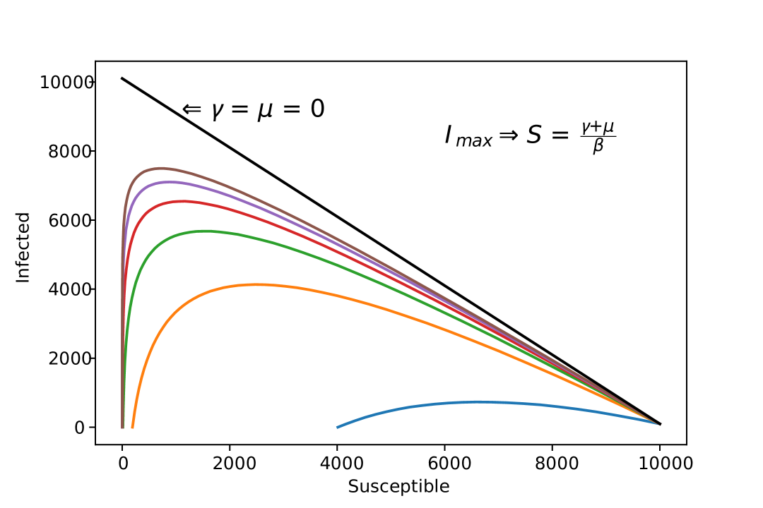
Hence, equation (8) may be written as
| (10) |
We can visualize here, that depending on the combination of and , reaches 0 before the entire population becomes infected (Figure 2).
Next, we may write in terms of and . For this purpose, we begin by dividing equation (1) by (3) and (1) by (4),
| (11) | |||
| (12) |
Adding these two equations and writing as , we get
| (13) |
Since (13) is a separable equation, the well-known solution is given by
| (14) | ||||
| (15) |
Therefore, can be written as
| (16) |
where we absorbed both constants and into . By the initial condition, we find that . To find and , we must derive (16) in time under the condition that it may return to equation (1). In this way, we see that
| (17) |
Solving this system,
| (19) | |||
| (20) |
Hence, can be finally written as
| (21) |
With this equation, see that as , does not approaches necessarily, depending on the recovery and death rates, does not reach .
The last important quantity extracted from this model is the basic reproduction number , given by [14]:
| (22) |
This quantity, is of vital importance of the study of a disease outbreak.
2.2 SEIRD
Another deterministic mathematical model possible is the SEIRD model, in which we consider the population of a given region as divided in 5 groups. At time , there are those who are susceptible to get infected , the ones who have already been exposed the virus but does not present symptoms yet , people who are already infected and present the symptoms , the ones that have already recovered from the disease and those who are dead due to the infection . This model is a good approximation to a short epidemic, so the population of a region is roughly constant throughout the epidemic period. Also, since this is a deterministic model, we assume to be a big number compared to the number of people associated with the infection of a single person. The final consideration is that we also assume that people that are recovered from the disease acquire immensity and does not become susceptible to become infected again.
The rate of infection is proportional to the number of people infected, , where the constant represents the effectiveness of the infection, the rate of cure , where is the probability of recovery and is the average time taken for an infected person to recover. Similarly the rate of death is , where is the probability of death, given by the CFR and is the average time taken for an infected person to die. Figure 3 carries an visual representation of the SEIRD model.
The differential equations representing the evolution of the populations are given by
| (23) | ||||
| (24) | ||||
| (25) | ||||
| (26) | ||||
| (27) |
We first turn our attention to the construction of an appropriate formula for calculating with this model. For that we follow the method derived on [20]. The study develops a mathematical generalization for writing depending on the type of epidemiological model. is defined as
| (28) |
where means the spectral radius of the matrix X, that is, the largest absolute eigenvalue. Both and are the matrices of the derivatives of the functions defining the behavior of the disease population, with respect to each population compartment.
To get to these matrices, we first note that the set of equations regarding the dynamics of the SEIRD model can be expressed as follow: Consider the vector of populations, that is where , , , and . Analogously, is the vector of the first derivatives. Then, we can write the dynamics of the populations as
| (29) |
where is the vector that relates the appearance of new infections on the disease populations due to contamination, and is the input and output of members in all populations due to all other causes, such as recovery from the disease, development of symptoms after an incubation period, etc. In our case, since all newly infected members go to the population
| (30) |
while
| (31) |
Now, we know that the situation of a disease free equilibrium (DFE), meaning no disease is happening, is achived by the vector , where . According now to [20] we can calculate and as
| (32) | |||
| (33) |
being the vector components of related to the populations with the disease, in our case and , and is the number of populations related to infectious beings. Here . Performing the derivatives, we conclude
| (35) | |||
| (36) |
The next step is to find the inverse matrix of , fortunately is a 2x2 matrix and the formula for it’s inverse is straightforward
| (37) |
and we proceed to the last step of combining in order to retrieve and find .
| (38) | |||
therefore, by computing the eingenvalues of we find
| (39) |
Having in our hands, we continue to the study of some behaviors of this model.
The set of equations describing the model is subjected to the initial conditions. When , , , , and , where is the initial number of infected, is the initial number of exposed in the population and no deaths or recoveries are assumed at .
2.3 Non-pharmaceutical intervention
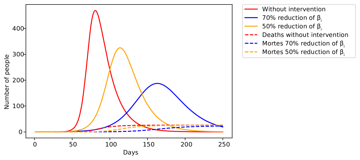
Without vaccines or efficient medicine against the disease, non-pharmaceutical interventions are the only effective way to prevent further increase of the pandemic [13]. These interventions take different approaches such as social distancing, social isolation and lockdown of the population. Despite the differences, they all carry the same objective, decreasing the infection rate . It is convenient to implement the effect of these interventions on the model, when making predictions. Here, we model this effect by a logistic function, where starts at a initial value and at some critical time a intervention is imposed and beta decreases to , where is the fraction of decreased by the intervention. In France, studies estimate that the intervention decreased by 77% [21], therefore in France.
| (40) |
where is a constant related to the time taken for the intervention to have the effect desired. Such model reconstruct the general behavior of interventions against the spread of the disease (Figure 4)
2.4 Age division
Since the case fatality rate (CFR) of COVID-19 is different among age groups [6, 7, 22], we propose here a modification on both models, including the age distribution of the population and the social aspects of close contact between members of the population. The modification is describe as follow: Each compartment is divided into age groups, where each -th group has a associated to it, that is, the probability of death associated to the -th age group. The parameter is now described as the average number of daily contacts between a member belonging to the -th age group to the -th age group, multiplied by the infection probability
| (41) | |||
| (42) |
where is called the social contact matrix and we included and inside now to place everything on the same sum. The age distribution among the population is retrieved from the UN prospects [23] and the social contact matrix for those countries was measured on previous studies [24, 25]. The specific contact matrix for the Republic of Korea was not found, however, [26] finds evidences of cultural clusters in the world, where countries belonging to the same cluster share cultural similarities; thus, we use this fact to justify the use of Hong Kong’s social contact matrix to describe the Republic of Korea. That way, we include cultural and population aspects for each of those countries, increasing the odds of a successful prediction. This type of model was used recently to describe the coronavirus outbreak on large cities in Brazil [27].
3 Comparing Adjustments
To test the SIRD and SEIRD model we first compare them to the pandemic crisis on the Republic of Korea, running a numerical solution for the differential equations (23) - (27) we adjust the general behavior of the populations to Korean data acquired from [28] since 15/02/2020. The data from the Republic of Korea consists of the infection curve and death curve. To prevent problems with initial guess on the fitting process, both models used the same values for the initial guess, except , which is found only on the SEIRD model. was also left as a free parameter of the adjustment instead of set to the total population of the country, which is justified by a limitation in both models, where the population is assumed homogeneously spread, which does not correspond to reality. Thus, does not represent the total population, instead it represents an effective population smaller than the total population, due to non-homogeneous distribution throughout the territory, the interpretation of as the disease evolves is discussed on the discussion session. The parameter was chosen to be , we considered a study which estimated that presyntomatic cases caused 44% of infections [29], while for we used an average of several clinical studies shown on table 1.
| incubation time | 95% confidence | Reference |
|---|---|---|
| 6.4 days | 5.6-7.7 | [30] |
| 5.2 days | 4.1-7 | [3] |
| 5 days | – | [31] |
| 4 days | – | [32] |
| 5.1 days | 4.5 - 5.8 | [33] |
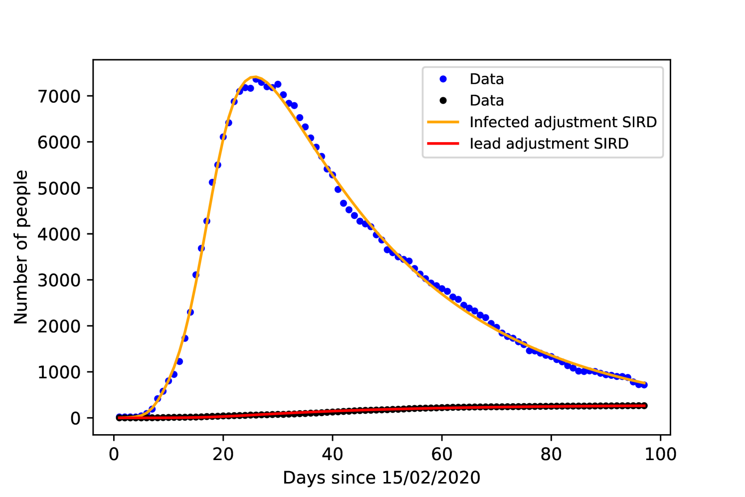
Since the Korean government did not impose a lockdown or social isolation, we set in both models. Figures 6 and 6 show the result of the fitting process and table 2 includes the acquired values for all parameters for each model.

| Parameter | SIRD | SEIRD |
|---|---|---|
| 0.9978 | 0.9978 | |
| 7.9 0.3 | 8 0.3 | |
| 29.6 0.2 | 28.8 0.2 | |
| 2 1 | 1 4 | |
| – | 62 57 | |
| 0.478 0.004 | 0.513 0.008 | |
| 11035 57 | 11218 48 |
The recovery time on both models is close to 8 days, while other studies such as [34] found 10 days. The time from symptoms onset to death was in both models close to 30 days, being 1 day shorter with the SEIRD model, [35] and [36] found or days.
Comparing the accuracy of the fitting with the data, both models resulted the same value of . The parameter presents a large margin of error, which is expected given the lack of real data concerning the exposed population.
| (43) | |||
| (44) |
4 Prediction Accuracy with Age Division
We now proceed to test the prediction accuracy of both models. We used the first third of the data for fitting both models and extracting parameters, after having the parameters, we compare the prediction for the next days with these parameters with the rest of the dataset.
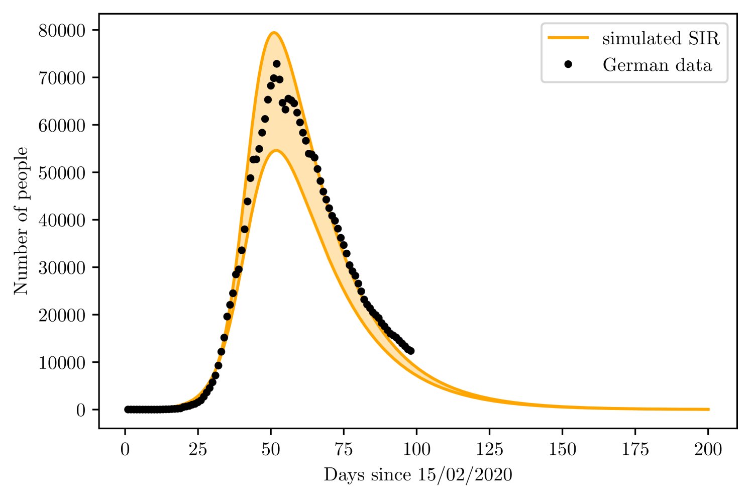
4.1 Germany
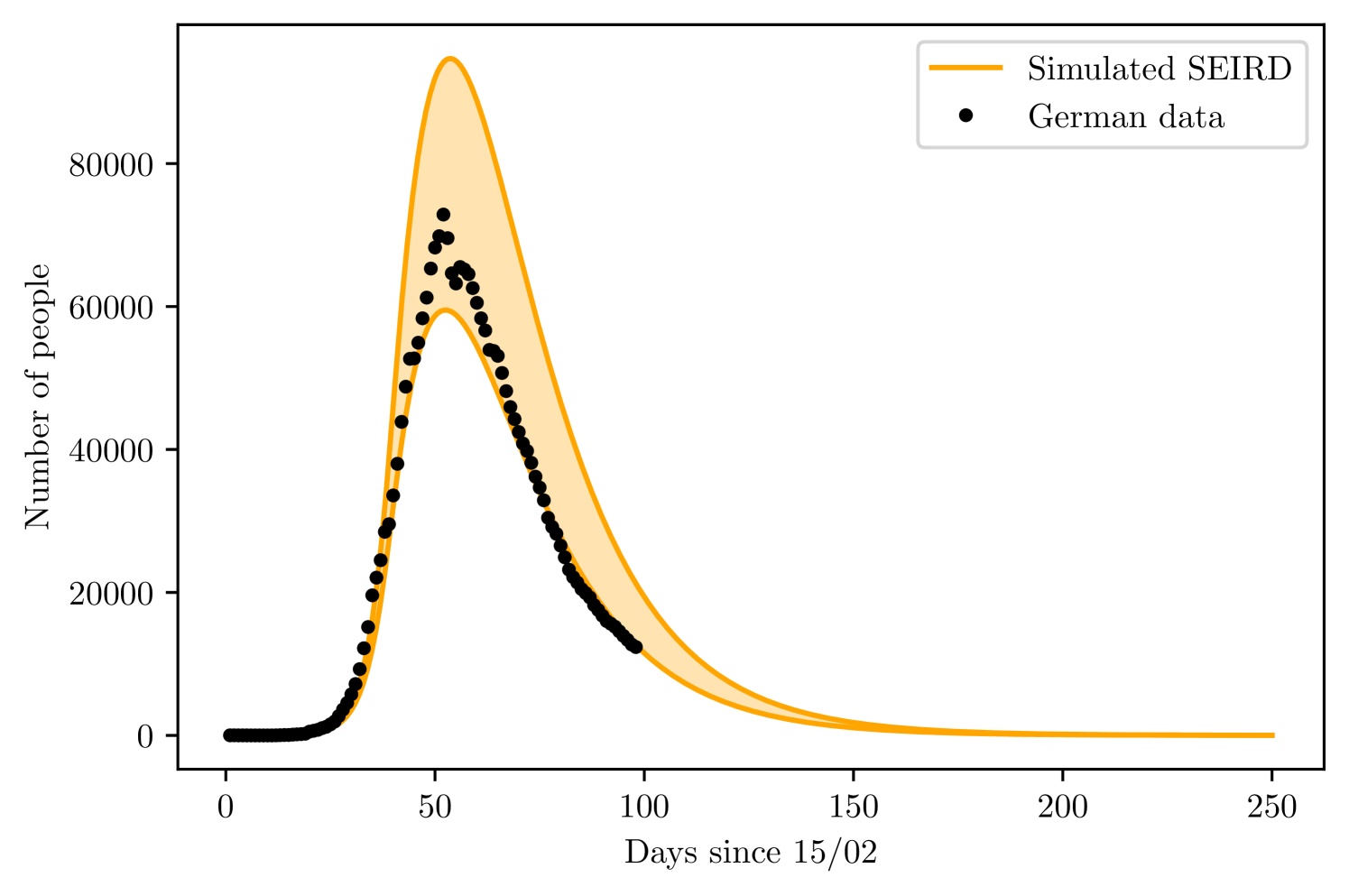
For Germany, the fitting data corresponds to the cases and deaths until 17th March. However, until the peak is reached, both models find presents very large margin of error for , to avoid this problem, we varied manually, from 0 to 10% of the local population; which was taken from a united nation prospect for the year of 2020 [23], at steps of 0.05%. At each step, we fit the initial data and reject the fitting if the value is lower than 0.995, this method for validating the goodness of a data adjustment had already been used for epidemiological models [41]. We than plotted the maximum and minimum acceptable fits to generate the margin of prediction, comparing it with the complete dataset. We also decided to use and according to clinical studies when performing the prediction, instead of leave them as free parameters for the fitting, was also determined a priori according to the first registered number on 15/02/2020. The resulting free parameters for fitting the training set are and .
With the SEIRD model, we found the maximum and minimum values of to be of the German population and of the German population. The parameter varied from 15.5% to 16.2%
Using the SIRD, leaving and as free parameters. The limit values of were and , while varied from to and from 11 to 30. Figures 8 and 8 show the result of both simulations, with the maximum and minimum curves. The shaded region is the region between and .
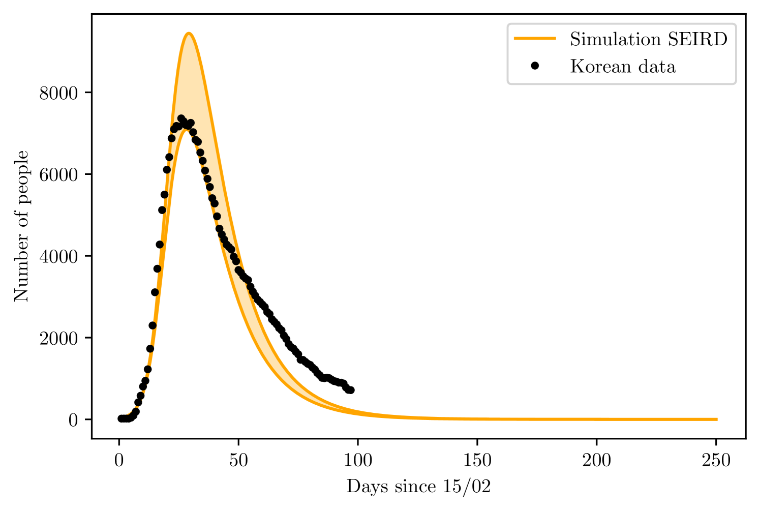
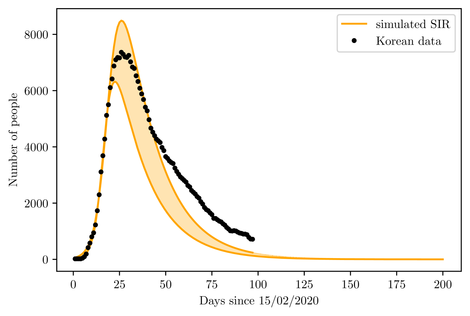
4.2 Korea
The training set consisted of 20 days, corresponding to the infections from 15/02 to 06/03. The SEIRD model found and of the total Korean population, while varied between 80 to 85%.
The simple SIRD model found and , went from 0.345 to 0.436, and was between 23 to 65. Figures 10 and 10 present the result for prediction of both models.
5 Discussion
When concerning the adjustment process for acquisition of parameters with both models, there were no difference on the accuracy of the fit, and both models yielded very close values for the parameters. However, is super estimated in both models, being slightly lower on the SEIRD model. The value of is acceptable inside the variation of clinical measures.
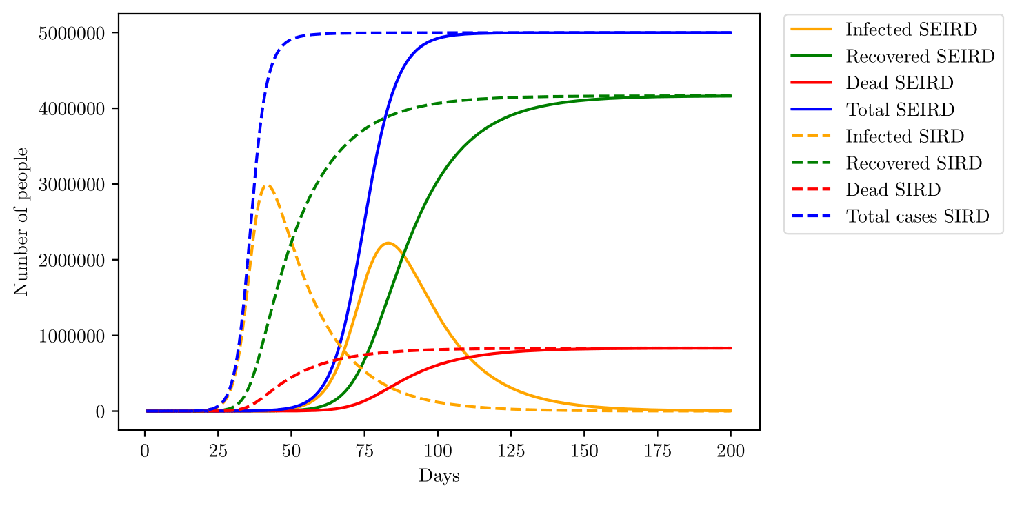
The SEIRD model yields a slower growth rate than the SIRD model, that might happen due to the incubation period on the SEIRD model, which slows down the propagation of the virus towards other individuals. The main difference between the growth rate predicted by both models is better visualized by figure 11, the action of the incubation period slows down the rate of infection, as seen by the adjustments, but also decreases the peak of infections. However, the cumulative numbers of infection, deaths and recoveries are the same.
could be understood as the population susceptible to the first pandemic wave, due to the non-homogeneous distribution of the population, not everyone is susceptible to the disease right at the start. With such an interpretation, tends to increase with time and approach the total population, here. Comparing predictions generated by the SIRD model with the SEIRD model with age division, the SEIRD model becomes a little more precise, although both simulations fail to predict the slower decrease of Korean data, that might be explained by an increase on as time passes, resulting in new cases registered and therefore, slowing down the rate of decrease. Such hypothesis is well acceptable since the Republic of Korea did not adopt any lockdown or social isolation measure, making the disease able to propagate towards other regions, increasing with time. Even with better prediction, the SEIRD model is far more complicated than the SIRD model and the use of the later should probably not compromise any data analysis. The same must hold true for simple SIR and SEIR models, when deaths are not a population to be accounted for, instead are just represented with a rate of removal for individuals.
The social isolation model developed here shows good results on the predictions, indicating that the description of should be close to reality. Here we find a huge advantage of the SEIRD model with age division in comparison with the SIRD model; by including age division, it is possible to simulate the effect of specific non-pharmaceutical interventions, such as school closure, which in principle would decrease and for the age groups between 0 to 19 years only. Another possibility is to include isolation of only elderly individuals. Several non-pharmaceutical measures have been already described in literature [42], other studies show how the total number of infected might be changed due to the efficiency of non-pharmaceutical measures [43].
Other models might present more complete analysis of the disease, including hospitalizations and even asymptomatic cases, which are difficult to track and seem to vary a lot from place to place, the Diamond Princess cruise ship found 17.9% of asymptomatic infections [44], while an airplane flight found 11.2% of cases being asymptomatic. An Italian village presented 50 to 70% of cases being asymptomatic [45]. There are yet the problem of assuring that the asymptomatic cases registered on studies are really asymptomatic and not presymtomatic, that is, are people still on the incubation period.
Of course, any mathematical model is only as good as the data allows, using mathematical models to describe the disease on countries with low testing rates might yield unrealistic predictions. For example, [46] estimates 86% of infections being undocumented on China, at the early stages of the outbreak.
Another consideration we did not take, was the possibility of reinfection, where individuals leave the recovered group and re-enter the susceptible compartment. However, since other coronaviruses belonging to the same genus betacoronavirus such as the SARS-CoV and the MERS-CoV does not present a high enough mutation rate to cause reinfection in short term [47], the only cause of reinfection would be the loss of antibodies to fight the virus; nevertheless, on both diseases, the infected person acquires antibodies enough to prevent reinfection for a period of 2 - 3 years [48]. With those considerations, we did not assume reinfection was probable on short-term. Future studies may be conducted to study the possibility of reinfection of individuals on the long-term.
6 Conclusion
Mathematical models of a disease outbreak such as the COVID-19 are able to predict the behavior of the infection. Both models have proved to be efficient tools for acquiring data and forecast the future situation. Despite the limitations, the models made it possible to achieve a value of in good agreement with other studies, providing evidence in favor of the validity of the model.
However, the present models do not take into consideration the spatial distribution of the population, reflecting on some uncertainties that made the window of prediction larger.
The age division does not change the prediction drastically, suggesting that in the case of a simple prediction or analysis, SIRD models are useful. The age division SEIRD model provides an advantage when requiring specific simulations on specific groups of the population.
References
- [1] Vineet D Menachery, Boyd L Yount Jr, Kari Debbink, Sudhakar Agnihothram, Lisa E Gralinski, Jessica A Plante, Rachel L Graham, Trevor Scobey, Xing-Yi Ge, Eric F Donaldson, et al. A sars-like cluster of circulating bat coronaviruses shows potential for human emergence. Nature medicine, 21(12):1508, 2015.
- [2] Roujian Lu, Xiang Zhao, Juan Li, Peihua Niu, Bo Yang, Honglong Wu, Wenling Wang, Hao Song, Baoying Huang, Na Zhu, et al. Genomic characterisation and epidemiology of 2019 novel coronavirus: implications for virus origins and receptor binding. The Lancet, 395(10224):565–574, 2020.
- [3] Qun Li, Xuhua Guan, Peng Wu, Xiaoye Wang, Lei Zhou, Yeqing Tong, Ruiqi Ren, Kathy SM Leung, Eric HY Lau, Jessica Y Wong, et al. Early transmission dynamics in wuhan, china, of novel coronavirus–infected pneumonia. New England Journal of Medicine, 2020.
- [4] World Health Organization et al. Coronavirus disease 2019 (covid-19): situation report, 67. 2020.
- [5] Marco Cascella, Michael Rajnik, Arturo Cuomo, Scott C Dulebohn, and Raffaela Di Napoli. Features, evaluation and treatment coronavirus (covid-19). In StatPearls [Internet]. StatPearls Publishing, 2020.
- [6] Vital Surveillances. The epidemiological characteristics of an outbreak of 2019 novel coronavirus diseases (covid-19)—china, 2020. China CDC Weekly, 2(8):113–122, 2020.
- [7] Zunyou Wu and Jennifer M McGoogan. Characteristics of and important lessons from the coronavirus disease 2019 (covid-19) outbreak in china: summary of a report of 72 314 cases from the chinese center for disease control and prevention. Jama, 2020.
- [8] Joseph T Wu, Kathy Leung, and Gabriel M Leung. Nowcasting and forecasting the potential domestic and international spread of the 2019-ncov outbreak originating in wuhan, china: a modelling study. The Lancet, 395(10225):689–697, 2020.
- [9] Jesús Fernández-Villaverde and Charles I Jones. Estimating and simulating a sird model of covid-19 for many countries, states, and cities. Technical report, National Bureau of Economic Research, 2020.
- [10] Kentaro Iwata and Chisato Miyakoshi. A simulation on potential secondary spread of novel coronavirus in an exported country using a stochastic epidemic seir model. Journal of Clinical Medicine, 9(4):944, 2020.
- [11] Affan Shoukat, Chad R Wells, Joanne M Langley, Burton H Singer, Alison P Galvani, and Seyed M Moghadas. Projecting demand for critical care beds during covid-19 outbreaks in canada. CMAJ, 192(19):E489–E496, 2020.
- [12] Patrick GT Walker, Charles Whittaker, Oliver Watson, M Baguelin, KEC Ainslie, S Bhatia, S Bhatt, A Boonyasiri, O Boyd, L Cattarino, et al. The global impact of covid-19 and strategies for mitigation and suppression. WHO Collaborating Centre for Infectious Disease Modelling, MRC Centre for Global Infectious Disease Analysis, Abdul Latif Jameel Institute for Disease and Emergency Analytics, Imperial College London, 2020.
- [13] Jonas Dehning, Johannes Zierenberg, F Paul Spitzner, Michael Wibral, Joao Pinheiro Neto, Michael Wilczek, and Viola Priesemann. Inferring change points in the spread of covid-19 reveals the effectiveness of interventions. Science, 2020.
- [14] Cleo Anastassopoulou, Lucia Russo, Athanasios Tsakris, and Constantinos Siettos. Data-based analysis, modelling and forecasting of the covid-19 outbreak. PloS one, 15(3):e0230405, 2020.
- [15] Sunhwa Choi and Moran Ki. Estimating the reproductive number and the outbreak size of covid-19 in korea. Epidemiology and Health, 42, 2020.
- [16] Pedro Henrique Pinheiro Cintra and Felipe Fontinele Nunes. Estimative of real number of infections by covid-19 on brazil and possible scenarios. medRxiv, 2020.
- [17] Marco Ferrante, Elisabetta Ferraris, and Carles Rovira. On a stochastic epidemic seihr model and its diffusion approximation. Test, 25(3):482–502, 2016.
- [18] Igor Nesteruk. Estimations of the coronavirus epidemic dynamics in south korea with the use of sir model. Preprint.] ResearchGate, 2020.
- [19] Igor Nesteruk. Statistics based predictions of coronavirus 2019-ncov spreading in mainland china. MedRxiv, 2020.
- [20] Pauline Van den Driessche and James Watmough. Reproduction numbers and sub-threshold endemic equilibria for compartmental models of disease transmission. Mathematical biosciences, 180(1-2):29–48, 2002.
- [21] Henrik Salje, Cécile Tran Kiem, Noémie Lefrancq, Noémie Courtejoie, Paolo Bosetti, Juliette Paireau, Alessio Andronico, Nathanaël Hoze, Jehanne Richet, Claire-Lise Dubost, et al. Estimating the burden of sars-cov-2 in france. Science, 2020.
- [22] Sijia Tian, Nan Hu, Jing Lou, Kun Chen, Xuqin Kang, Zhenjun Xiang, Hui Chen, Dali Wang, Ning Liu, Dong Liu, et al. Characteristics of covid-19 infection in beijing. Journal of Infection, 2020.
- [23] Department of Economic and Social Affairs. World population prospects 2019, 2019.
- [24] Joël Mossong, Niel Hens, Mark Jit, Philippe Beutels, Kari Auranen, Rafael Mikolajczyk, Marco Massari, Stefania Salmaso, Gianpaolo Scalia Tomba, Jacco Wallinga, et al. Social contacts and mixing patterns relevant to the spread of infectious diseases. PLoS medicine, 5(3), 2008.
- [25] Kathy Leung, Mark Jit, Eric HY Lau, and Joseph T Wu. Social contact patterns relevant to the spread of respiratory infectious diseases in hong kong. Scientific reports, 7(1):1–12, 2017.
- [26] Vipin Gupta, Paul J Hanges, and Peter Dorfman. Cultural clusters: Methodology and findings. Journal of world business, 37(1):11–15, 2002.
- [27] Tarcisio M Rocha Filho, Fabiana S Ganem dos Santos, Victor B Gomes, Thiago AH Rocha, Julio HR Croda, Walter M Ramalho, and Wildo N Araujo. Expected impact of covid-19 outbreak in a major metropolitan area in brazil. medRxiv, 2020.
- [28] WorldMeters. Coronavirus cases, 2020.
- [29] Xi He, Eric HY Lau, Peng Wu, Xilong Deng, Jian Wang, Xinxin Hao, Yiu Chung Lau, Jessica Y Wong, Yujuan Guan, Xinghua Tan, et al. Temporal dynamics in viral shedding and transmissibility of covid-19. Nature medicine, pages 1–4, 2020.
- [30] Jantien A Backer, Don Klinkenberg, and Jacco Wallinga. Incubation period of 2019 novel coronavirus (2019-ncov) infections among travellers from wuhan, china, 20–28 january 2020. Eurosurveillance, 25(5), 2020.
- [31] Natalie M Linton, Tetsuro Kobayashi, Yichi Yang, Katsuma Hayashi, Andrei R Akhmetzhanov, Sung-mok Jung, Baoyin Yuan, Ryo Kinoshita, and Hiroshi Nishiura. Incubation period and other epidemiological characteristics of 2019 novel coronavirus infections with right truncation: a statistical analysis of publicly available case data. Journal of Clinical Medicine, 9(2):538, 2020.
- [32] Wei-jie Guan, Zheng-yi Ni, Yu Hu, Wen-hua Liang, Chun-quan Ou, Jian-xing He, Lei Liu, Hong Shan, Chun-liang Lei, David SC Hui, et al. Clinical characteristics of coronavirus disease 2019 in china. New England Journal of Medicine, 2020.
- [33] Stephen A Lauer, Kyra H Grantz, Qifang Bi, Forrest K Jones, Qulu Zheng, Hannah R Meredith, Andrew S Azman, Nicholas G Reich, and Justin Lessler. The incubation period of coronavirus disease 2019 (covid-19) from publicly reported confirmed cases: estimation and application. Annals of internal medicine, 2020.
- [34] Adam Bernheim, Xueyan Mei, Mingqian Huang, Yang Yang, Zahi A Fayad, Ning Zhang, Kaiyue Diao, Bin Lin, Xiqi Zhu, Kunwei Li, et al. Chest ct findings in coronavirus disease-19 (covid-19): relationship to duration of infection. Radiology, page 200463, 2020.
- [35] Qiurong Ruan, Kun Yang, Wenxia Wang, Lingyu Jiang, and Jianxin Song. Clinical predictors of mortality due to covid-19 based on an analysis of data of 150 patients from wuhan, china. Intensive care medicine, pages 1–3, 2020.
- [36] Pierfrancesco Barbariol Antonino Bella Stefania Bellino Eva Benelli Luigi Palmieri, Xanthi Andrianou. Characteristics of sars-cov-2 patients dying in italy. report based on available data on may 14th. 2020.
- [37] Shi Zhao, Qianyin Lin, Jinjun Ran, Salihu S Musa, Guangpu Yang, Weiming Wang, Yijun Lou, Daozhou Gao, Lin Yang, Daihai He, et al. Preliminary estimation of the basic reproduction number of novel coronavirus (2019-ncov) in china, from 2019 to 2020: A data-driven analysis in the early phase of the outbreak. International Journal of Infectious Diseases, 92:214–217, 2020.
- [38] Ying Liu, Albert A Gayle, Annelies Wilder-Smith, and Joacim Rocklöv. The reproductive number of covid-19 is higher compared to sars coronavirus. Journal of travel medicine, 2020.
- [39] Sheng Zhang, MengYuan Diao, Wenbo Yu, Lei Pei, Zhaofen Lin, and Dechang Chen. Estimation of the reproductive number of novel coronavirus (covid-19) and the probable outbreak size on the diamond princess cruise ship: A data-driven analysis. International Journal of Infectious Diseases, 93:201–204, 2020.
- [40] Jonathan M Read, Jessica RE Bridgen, Derek AT Cummings, Antonia Ho, and Chris P Jewell. Novel coronavirus 2019-ncov: early estimation of epidemiological parameters and epidemic predictions. medRxiv, 2020.
- [41] SY Tang, YN Xiao, ZH Peng, and HB Shen. Prediction modeling with data fusion and prevention strategy analysis for the covid-19 outbreak. Zhonghua liu xing bing xue za zhi= Zhonghua liuxingbingxue zazhi, 41(4):480–484, 2020.
- [42] Feng Lin, Kumar Muthuraman, and Mark Lawley. An optimal control theory approach to non-pharmaceutical interventions. BMC infectious diseases, 10(1):32, 2010.
- [43] Neil M Ferguson, Daniel Laydon, Gemma Nedjati-Gilani, Natsuko Imai, Kylie Ainslie, Marc Baguelin, Sangeeta Bhatia, Adhiratha Boonyasiri, Zulma Cucunubá, Gina Cuomo-Dannenburg, et al. Impact of non-pharmaceutical interventions (npis) to reduce covid-19 mortality and healthcare demand. 2020.
- [44] Kenji Mizumoto, Katsushi Kagaya, Alexander Zarebski, and Gerardo Chowell. Estimating the asymptomatic proportion of coronavirus disease 2019 (covid-19) cases on board the diamond princess cruise ship, yokohama, japan, 2020. Eurosurveillance, 25(10):2000180, 2020.
- [45] Michael Day. Covid-19: identifying and isolating asymptomatic people helped eliminate virus in italian village. Bmj, 368:m1165, 2020.
- [46] Ruiyun Li, Sen Pei, Bin Chen, Yimeng Song, Tao Zhang, Wan Yang, and Jeffrey Shaman. Substantial undocumented infection facilitates the rapid dissemination of novel coronavirus (sars-cov2). Science, 2020.
- [47] Zhongming Zhao, Haipeng Li, Xiaozhuang Wu, Yixi Zhong, Keqin Zhang, Ya-Ping Zhang, Eric Boerwinkle, and Yun-Xin Fu. Moderate mutation rate in the sars coronavirus genome and its implications. BMC evolutionary biology, 4(1):21, 2004.
- [48] Wei Liu, Arnaud Fontanet, Pan-He Zhang, Lin Zhan, Zhong-Tao Xin, Laurence Baril, Fang Tang, Hui Lv, and Wu-Chun Cao. Two-year prospective study of the humoral immune response of patients with severe acute respiratory syndrome. The Journal of infectious diseases, 193(6):792–795, 2006.