Maxima of Two Random Walks: Universal Statistics of Lead Changes
Abstract
We investigate statistics of lead changes of the maxima of two discrete-time random walks in one dimension. We show that the average number of lead changes grows as in the long-time limit. We present theoretical and numerical evidence that this asymptotic behavior is universal. Specifically, this behavior is independent of the jump distribution: the same asymptotic underlies standard Brownian motion and symmetric Lévy flights. We also show that the probability to have at most lead changes behaves as for Brownian motion and as for symmetric Lévy flights with index . The decay exponent varies continuously with the Lévy index for , while when .
pacs:
05.40.Jc, 05.40.Fb, 02.50.Cw, 02.50.EyI Introduction
Extreme values play a crucial role in science, technology, and engineering. They are linked to rare events, large deviations, and optimization: minimizing a Lagrangian, for instance, is a frequent task in physics. Extreme values also provide an important characterization of random processes, and the study of extreme values is a significant area in statistics and probability theory Gumbel ; rse ; abn ; vbn ; jk ; mrfky ; gw .
For a scalar random process, there are two extreme values—the maximum and the minimum. It suffices to consider the maximum. Take the most basic random process, Brownian motion Levy ; IM65 ; BM:book . By Brownian motion we always mean standard Brownian motion, namely the one-dimensional Brownian process that starts at the origin: with . For the Brownian motion, the maximum process is defined by
| (1) |
This maximum process is non-trivial as demonstrated by the absence of stationarity—the increment depends on both and . In contrast, the position increment, , depends only on ; this stationarity is a crucial simplifying feature of Brownian motion. Still, the maximum process (1) has a number of simple properties, e.g. the probability density of the maximum is a one-sided Gaussian
| (2) |
The joint probability distribution of the position and maximum, and , also admits an elegant representation DC
| (3) |
This lesser-known formula, which was discovered by Lévy Levy , proves useful in many situations (see IM65 ; bk14a ); it can be derived using the reflection property of Brownian motion.
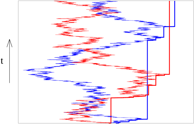
In this article, we study the leapfrogging of the maxima of two Brownian motions (see Fig. 1). The probability that one maximum exceeds another during the time interval was investigated only recently bk14 ; JRF . Here we explore additional features of the interplay between two Brownian maxima. When appropriate, we emphasize the universality of our results, e.g. some of our findings apply to rather general Markov processes, e.g. to arbitrary symmetric Lévy flights.
One of our main results is that the average number of lead changes between the two Brownian maxima exhibits a universal logarithmic growth
| (4) |
in the long-time limit. This behavior holds for random walks, and more generally for identical symmetric Lévy flights.
We also study the probability to have exactly lead changes during the time interval , see Fig. 1. We show that in the case of identical symmetric Lévy flights, the probability decays according to
| (5) |
The persistence exponent , that characterizes the probability that the lead does not change, depends only on the Lévy index . We evaluate numerically the quantity for .
This paper is organized as follows. In Sect. II we establish the growth law (4). First, we provide a heuristic derivation (Sect. II.1) relying on the probability densities (2)–(3). We also mention the generalization to two random walks with different diffusion coefficients. In Sect. II.2 we establish a link with first-passage time densities and the arcsine law, and we employ it to provide a more rigorous and more general derivation of (4). In Sect. III we study the statistics of lead changes for symmetric Lévy processes, particularly symmetric Lévy flights with index . The average number of lead changes is shown to exhibit the same universal leading asymptotic behavior (4) independent of the Lévy index. In Sect. IV we show that for identical symmetric random walks the probability to observe exactly lead changes between the maxima behaves as . We conclude with a discussion (Sect. V).
II The average number of lead changes
The question about the distribution of the number of lead changes of Brownian particles is ill-defined if one considers the positions—there is either no changes or infinitely many changes. The situation is different for the maxima: the probability density to have exactly changes during the time interval is a well-defined quantity if the initial positions differ. Discretization is still necessary in simulations. The discrete-time framework also simplifies the heuristic reasoning which we employ below. The corresponding results for the continuous-time case follows from the central-limit theorem: a random walk with a symmetric jump distribution that has a finite variance converges to a Brownian motion.
Thus, we consider two discrete time random walks on a one-dimensional line. The position of each walk evolves according to
| (6) |
The displacements are drawn independently from the same probability density which is assumed to be symmetric, and hence . We set the variance to unity, . Further, we always assume that the walk starts at the origin . The probability distribution of its position becomes Gaussian
| (7) |
in the long-time limit. The maximal position of the walk during the time interval is
| (8) |
The probability distribution of the maximum is given by (2), and the joint position-maximum distribution is given by (3).
In the following, we consider two identical random walkers. We assume that both walkers start at the origin, . Denote by and the positions of the walkers and by and the corresponding maxima. If the first walker is considered to be the leader. If the notion of the leader is ambiguous. This happens at , and we postulate that the first walker is the original leader. There are no lead changes as long as both walkers remain in the half-line. Once the walkers spend time in the half-line, the identity of the leader can be ambiguous if the probability density is discrete, e.g.,
| (9) |
In the following, we tacitly assume that the probability density does not contain delta functions, so once the two maxima become positive they remain distinct.
Eventually the maximum of the second walker will overtake that of the first and the second walker turns into the leader. Yet, at some later moment, the leadership will change again. This leapfrogging proceeds indefinitely. How does the average number of lead changes vary with time? What is the distribution of the number of lead changes? In this section we answer the first question. First, we provide a derivation of the asymptotic growth law (4) using heuristic arguments.
II.1 Heuristic arguments
We now argue that the average number of lead changes exhibits the logarithmic growth (4). Let and the lead changes soon after that. We use the shorthand notation . The probability density for this quantity is given by (2). We are interested in the asymptotic behavior () and in this regime, the random walker is generally far behind the maximum. This behavior is intuitively obvious, and it can be made quantitative—using (3) we compute the average size of the gap between the maximum and the position
| (10) | |||||
The second maximum can overtake the first if is close to . Since , both and are close to and the probability of this event is
| (11) |
Once the second particle reaches the leading maximum it will overtake it given that the first particle is typically far behind, see (10). Therefore, the lead changes with rate
Integrating over all possible yields
| (12) |
which gives the announced growth law (4).
The average (4) already demonstrates that the lead changing process is not Poissonian. For a Poisson process, the probability to have exactly lead changes is fully characterized by the average :
| (13) |
This distribution would imply that the probability of having no lead change decays as , that is, slower than the behavior which has been established analytically bk14 ; JRF .
It is straightforward to generalize equation (4) to the situation where the two random walks have different diffusion coefficients, denoted by and . By repeating the steps above, we get
| (14) |
In particular, in the limit when one of the particles diffuses much more slowly than the other, , we have .
II.2 First-passage analysis
Here, we present an alternative approach which complements the heuristic arguments given in Sect. II.1. This approach is formulated in continuous time, and it accounts for the universality observed in the numerical simulations (see Fig. 3).
If , the probability that becomes the leader in the interval is given by the probability that the first-passage time of at level is in . Let us write for the first-passage density, and recall that the density of the maximum, is given by (2). By integrating over , we obtain the average rate of lead changes as a first-passage equation
| (15) |
The multiplicative factor on the right-hand side of (15) takes into account that could have been the leader. In the case of Brownian motion, the first-passage density is known SR_book , e.g. it can be derived using the method of images. This allows one to compute the integral in (15).
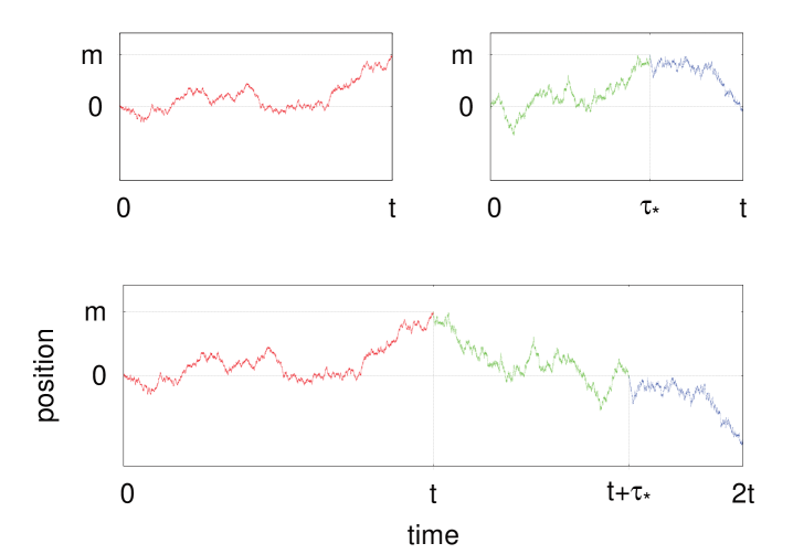
Interestingly, one can evaluate the integral in Eq. (15) without reference to the explicit forms of and . This evaluation uses path transformations in the same spirit as the well-known Verwaat construction for Brownian excursions Vervaat . One notices that the integrand in (15) corresponds to the product of densities associated with two independent paths: (i) a path first hitting at time , and (ii) a path having on a maximum equal to attained at some time . One then establishes a bijection between pairs of such paths and paths of duration , as illustrated in Fig. 2. This path transformation procedure produces paths of duration attaining their maximum at time , and having a non-positive final value.
When integrating over the product , one therefore obtains one half of the probability density associated with Brownian paths of duration attaining their maximum at time . This density is easily derived from the famous arcsine law Levy2 ; Levy , which states that the probability density for the time at which a Brownian motion attains its maximum over a fixed time interval is given by . One thus obtains
| (16) |
By combining (16) with (15), one recovers the heuristic prediction (12) and confirms . Moreover, the derivation is now sufficiently general as it applies to all random walks with symmetric jump distributions. Hence the leading asymptotic behavior (4) does not depend on the details of the (symmetric) jump distribution, in full agreement with the universality of the amplitude observed in numerical simulations. The first-passage equation and path transformation procedure can be applied to random walks that do not converge to Brownian motion, as discussed in the next section.
III Lévy flights
Brownian motion belongs to a family of (symmetric) Lévy processes Levy ; Bertoin ; DGNH ; LPA . These processes are stationary, homogeneous and stable. In a discrete time realization, a Lévy process becomes a Lévy flight. Lévy flights are ubiquitous in Nature, see Man82 ; BG90 ; BD97 ; SM . Here, we examine lead changes of the maxima of two identical Lévy flights. For Lévy flights, the jump distribution has a broad tail, and the Lévy index quantifies this tail, as . For simplicity, we choose the purely algebraic jump distribution,
| (17) |
When , Lévy flights are equivalent to an ordinary random walk. For true Lévy flights ; in this range the variance diverges. For even the average jump length becomes infinite. Generally for the displacement scales as .
We now show that the average number of lead changes exhibits logarithmic growth. Denote by the probability density of the maximum process and by the density of the first passage time at level . Following the same reasoning as in Sect. II.2, we write for the rate at which lead changes take place:
| (18) |
We now invoke the scaling properties of Lévy flights
| (19) |
These scaling forms reflect that the maximum process is -stable and the first-passage time process is -stable. Combining (18) and (19) we get
Consequently, the average number of lead changes grows logarithmically with time,
| (20) |
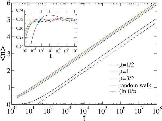
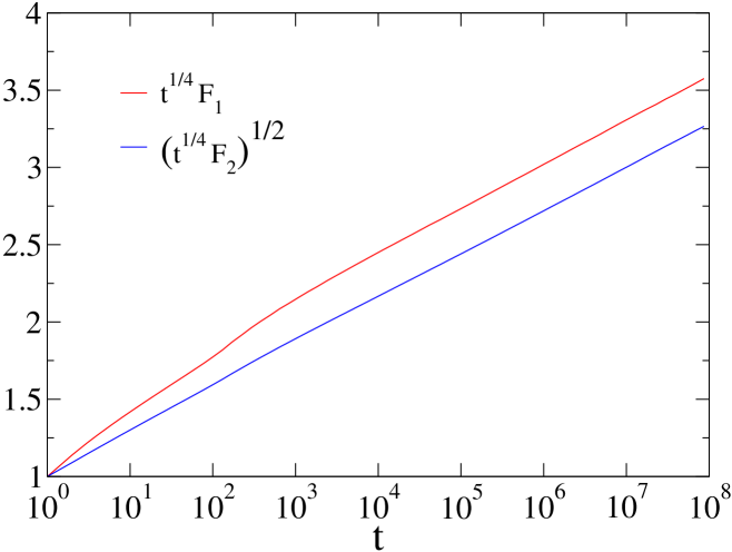
Our numerical simulations confirm that for identical random walks on a line, and even for random walks on the lattice with the discrete jump distribution (9), the amplitude is independent of the details of the jump distribution. Furthermore, the universality continues to hold for the Lévy flights, so independent of the Lévy index . This is confirmed by numerical simulations (see Fig. 3).
The universality can be understood by noting that the path transformation procedure described at the end of the previous section, as well as the arcsine law, are valid for Lévy flights. The key requirements are to have cyclic exchangeability of the jumps (which is guaranteed when these are independent and identically distributed), a continuous and symmetric jump distribution, and a certain type of regularity for the supremum, see F68b ; CUB ; Bertoin ; LPA . The validity of the arcsine law implies that we can use (16). Thus the leading asymptotic (4) holds for a wide class of symmetric Lévy processes, and in particular, symmetric Lévy flights.
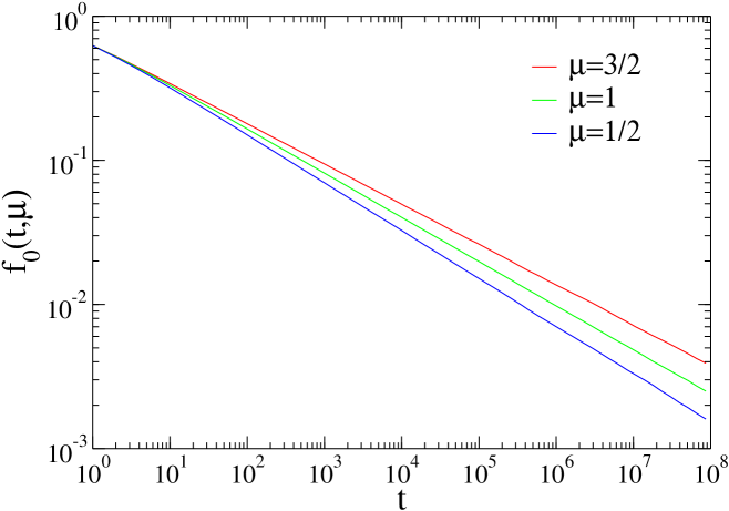
Next, we examine the probability that there are no lead changes till time . Our simulations show that this probability decays algebraically (see Fig. 4):
| (21) |
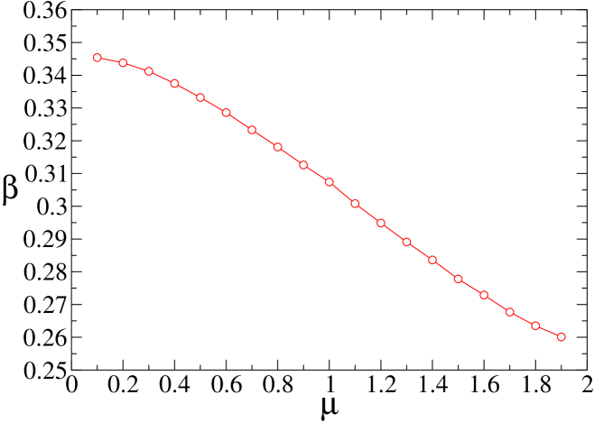
The persistence exponent varies continuously with , namely is a monotonically decreasing function of , see Fig. 5. For , Lévy flights are equivalent to ordinary random walks, so for .
In the marginal case , the mean-square displacement has a logarithmic enhancement over the classic diffusive growth, . Consequently, the convergence toward the ultimate asymptotic behavior is very slow near . Our numerical simulations suggest that in the marginal case , there may be a logarithmic correction to the algebraic decay (21).
IV Distribution of the number of lead changes
We now focus on the probability to have exactly lead changes until time . For two identical random walks, the probability that there are no lead changes decays as in the long-time limit bk14 ; JRF . Since is the probability that the -st lead change takes place after time , the probability density for the -st lead change to occur at time is given by . In particular, from , one can write down the conditional probability density of the time of the next lead change, given that it takes place after time :
| (22) |
Furthermore, the quantity is the probability that the first lead change occurs at some time and that the next one occurs at some time . The probability density associated with such a configuration is simply proportional to
Integrating over [we could introduce a cut-off , but this is akin to a discretization of time, so in the large limit we might as well set ], we find
Hence, there is a logarithmic enhancement of the probability to have one lead change compared with having none. The above argument can be generalized to arbitrary to yield
| (23) |
One can establish this general behavior by induction:
Thus, there are logarithmic corrections for all .
We probed the behavior of the cumulative distribution using numerical simulations. The quantity is the probability that the number of lead changes in time interval does not exceed . The dominant contribution to is provided by and hence
| (24) |
For Lévy flights, the distribution of the number of lead changes can be established in a similar manner. Using (21) and following the derivation of (23) we get
| (25) |
where is the aforementioned persistence exponent. Using numerical simulations, we verified that (25) holds for and for a few representative values of the Lévy index in the range.
V Discussion
The simplest model of correlated random variables is a one-dimensional discrete-time random walk. Its maximum evolves by a random process that exhibits a number of remarkable features. Some of these properties are classical Levy ; IM65 ; BM:book , while others were discovered only recently bk14a ; MZ08 ; MMS13 ; GMS14 . For instance, the probability distribution for the total number of distinct maximal values (records) achieved by the walk is universal MZ08 , i.e., independent of the details of the jump distribution, as long as the jump distribution is symmetric and not discrete. This universality also holds for symmetric Lévy flights, and in fact, it is rooted in the Sparre Andersen theorem SA54 . In the case of multiple identical random walks, the total number of records has been investigated in WMS .
In this article, we studied a sort of “competition” between maxima of two identical random walks. In particular, we examined the average number of lead changes and the probability to have exactly changes. We found that the average number of lead changes exhibits a universal logarithmic growth (4). This asymptotic behavior also holds for symmetric Lévy flights with arbitrary index. In contrast, the probability distribution is not universal: the persistence exponent in (25) depends on the Lévy index . The most interesting challenge for future work is to determine analytically the continuously varying exponent in the range .
One natural generalization of the competing maxima problem is to an arbitrary number of identical random walks or Lévy flights. We expect that the average number of lead changes among the maxima of identical random walkers still exhibits a universal logarithmic growth, albeit with a -dependent prefactor. Another quantity of interest is the survival probability that Lévy maxima remain ordered, , for . Based on (21), we anticipate that the probability decays algebraically,
| (26) |
Similar algebraic decays with -dependent exponents describe the probability that the positions of random walks remain perfectly ordered, the probability that one random walk remains the leader, etc. KM59 ; mef ; BG ; G99 ; bjmkr ; bk-mult .
For , the exponent appearing in (26) is our basic persistence exponent: . The exponents do not depend on when , i.e., for random walks. For ordinary random walks, the exponents were studied numerically in bk14 , while approximate values for these exponents were computed in bkl .
Generally one would like to explore the statistics of ordering and lead changes for a collection of random variables. Even the case of Markovian random variables is far from understood. Non-Markovian random variables appear intractable, but sometimes the progress is feasible due to hidden connection to Markovian processes. For instance, in the case of Brownian maxima the first-passage processes are Markovian. This allows one to use results from classical fluctuation theory to derive the persistence exponent , see JRF , and yields another derivation of the logarithmic growth of the average number of lead changes CKK . For Lévy flights, however, the existence of leapovers at the first passage time of certain points KLCKM leads to a breakdown of this approach. New results in this direction represent challenges for future work.
Acknowledgments
We benefited from discussions with S. N. Majumdar. Two of us (PLK and JRF) thank the Galileo Galilei Institute for Theoretical Physics for hospitality during the program on “Statistical Mechanics, Integrability and Combinatorics” and the INFN for partial support. The work of EBN was supported through US-DOE grant DE-AC52-06NA25396.
References
- (1) E. I. Gumbel, Statistics of Extremes (Dover, New York 2004).
- (2) R. S. Ellis, Entropy, Large Deviations, and Statistical Mechanics (Springer, Berlin 2005).
- (3) B. C. Arnold, N. Balakrishnan and H. N. Nagraja, Records (Wiley-Interscience, 1998).
- (4) V. B. Nevzorov, Records: Mathematical Theory, Translation of Mathematical Monographs 194 (American Mathematical Society, Providence, RI, 2001).
- (5) J. Krug, J. Stat. Mech. P07001 (2007).
- (6) S. N. Majumdar, J. Randon-Furling, M. J. Kearney, and M. Yor, J. Phys. A 41, 365005 (2008).
- (7) G. Wergen, J. Phys. A 46, 223001 (2013).
- (8) P. Lévy, Processus Stochastiques et Mouvement Brownien (Gauthier-Villars, Paris, 1948).
- (9) K. Itô and H. P. McKean, Diffusion Processes and Their Sample Paths (Springer, New York, 1965).
- (10) P. Mörters and Y. Peres, Brownian Motion (Cambridge: Cambridge University Press, 2010).
- (11) In Eqs. (2)–(3), we set the diffusion coefficient to ; the general case of an arbitrary diffusion coefficient is recovered by the transformation .
- (12) E. Ben-Naim and P. L. Krapivsky, J. Phys. A 47, 255002 (2014).
- (13) E. Ben-Naim and P. L. Krapivsky, Phys. Rev. Lett. 113, 030604 (2014).
- (14) J. Randon-Furling, EPL 109, 40015 (2015).
- (15) S. Redner, A Guide to First-Passage Processes (Cambridge University Press, Cambridge, 2001).
- (16) W. Vervaat, Ann. Probab. 7, 143 (1979).
- (17) P. Lévy, Compositio Mathematica 7, 283 (1940).
- (18) J. Bertoin, Lévy Processes (Cambridge University Press, Cambridge, 1996).
- (19) B. Dybiec, E. Gudowska-Nowak, and P. Hänggi, Phys. Rev. E 73, 046104 (2006).
- (20) A. E. Kyprianou, Fluctuations of Lévy Processes with Applications (Springer-Verlag, New York, 2014).
- (21) B. Mandelbrot, The Fractal Geometry of Nature (W. H. Freeman, New York, 1982).
- (22) J.-P. Bouchaud and A. Georges, Phys. Rept. 195, 127 (1990).
- (23) B. Derrida, Physica D 107, 186 (1997).
- (24) S. N. Majumdar, Physica A 389, 4299 (2010).
- (25) W. Feller, An Introduction to Probability Theory and its Applications, Vol. II (Wiley, New York, 1968).
- (26) L. Chaumont and G. Uribe Bravo, in: XI Symposium on Probability and Stochastic Processes (Springer International Publishing, 2015).
- (27) S. N. Majumdar and R. M. Ziff, Phys. Rev. Lett. 101, 050601 (2008).
- (28) S. N. Majumdar, P. Mounaix, and G. Schehr, Phys. Rev. Lett. 111, 070601 (2013).
- (29) C. Godrèche, S. N. Majumdar, and G. Schehr, J. Phys. A 47, 255001 (2014).
- (30) E. Sparre Andersen, Math. Scand. 1, 263 (1953); ibid. 2, 195 (1954).
- (31) G. Wergen, S. N. Majumdar, and G. Schehr, Phys. Rev. E 86, 011119 (2012).
- (32) S. P. Karlin and G. MacGregor, Pacific. J. Math. 9, 1141 (1959).
- (33) M. E. Fisher, J. Stat. Phys. 34, 667 (1984).
- (34) M. Bramson and D. Griffeath, in: Random Walks, Brownian Motion, and Interacting Particle Systems: A Festshrift in Honor of Frank Spitzer, eds. R. Durrett and H. Kesten (Birkhäuser, Boston, 1991).
- (35) D. J. Grabiner, Ann. Inst. Poincare: Prob. Stat. 35, 177 (1999).
- (36) P. L. Krapivsky and S. Redner, J. Phys. A 29, 5347 (1996); D. ben-Avraham, B. M. Johnson, C. A. Monaco, P. L. Krapivsky, and S. Redner, J. Phys. A 36, 1789 (2003).
- (37) E. Ben-Naim and P. L. Krapivsky, J. Phys. A 43, 495008 (2010).
- (38) E. Ben-Naim, P. L. Krapivsky, and N. W. Lemons, Phys. Rev. E 92, 062139 (2015).
- (39) K.L. Chung and M. Kac, Mem. Amer. Math. Soc. 6, 11 (1951); K.L. Chung and M. Kac, Ann. Math. 57, 604 (1953); H. Kesten, Indiana Univ. Math. J. 12, 391 (1963). Details of the derivation of (4) using the methods developed in these references will be published elsewhere.
- (40) T. Koren, M. A Lomholt, A. V. Chechkin, J. Klafter, and R. Metzler, Phys. Rev. Lett. 99, 160602 (2007).