Maximal diameter theorem for directed graphs of positive Ricci curvature

Ryunosuke Ozawa Department of Mathematics, National Defense Academy of Japan, 1-10-20 Hashirimizu, Yokosuka, 239-8686, Japan rozawa@nda.ac.jp , Yohei Sakurai Department of Mathematics, Saitama University, 255 Shimo-Okubo, Sakura-ku, Saitama-City, Saitama, 338-8570, Japan ysakurai@rimath.saitama-u.ac.jp and Taiki Yamada Shimane University, 1060 Nishikawatsu-cho, Matsue, Shimane, 690-8504, Japan taiki_yamada@riko.shimane-u.ac.jp

(Date: April 22, 2021)

Abstract.

In a previous work, the authors [15] have introduced a Lin-Lu-Yau type Ricci curvature for directed graphs, and obtained a diameter comparison of Bonnet-Myers type. In this paper, we investigate rigidity properties for the equality case, and conclude a maximal diameter theorem of Cheng type.

Key words and phrases:

Directed graph; Ricci curvature; Comparison geometry; Diameter; Spectrum

2010 Mathematics Subject Classification:

Primary 05C20, 05C12, 05C81, 53C21, 53C23

1. Introduction

For a Riemannian manifold of positive Ricci curvature, the Bonnet-Myers theorem asserts that its diameter is bounded from above by that of a corresponding standard sphere. Moreover, the Cheng maximal diameter theorem says that the equality in Bonnet-Myers theorem holds if and only if it is isometric the sphere. In this article, we are concerned with their discrete analogues. In [15], the authors have introduced a Lin-Lu-Yau type Ricci curvature for directed graphs, and produced a Bonnet-Myers type diameter comparison theorem. We now aim to examine its equality case. In that case, we derive several results on geometric structure, and some analytic results for the Chung Laplacian.

1.1. Main results

Recently, there are some attempts to introduce the notion of the Ricci curvature for discrete spaces, and the Ricci curvature for (undirected) graphs introduced by Lin-Lu-Yau [11] is one of the well-studied objects (see also a pioneering work of Ollivier [14]). It is well-known that a lower Ricci curvature bound of them leads us to various geometric and analytic consequences (see e.g., [1], [2], [3], [7], [9], [11], [13], [16], and so on). In [11], they have provided a discrete analogue of Bonnet-Myers theorem in Riemannian geometry. Furthermore, Cushing et al. [7] have established that of Cheng maximal diameter theorem for regular graphs. They have investigated their geometric structure in the equality case, and concluded a classification of self-centered regular graphs based on [10].

In [15], the authors have generalized the Lin-Lu-Yau Ricci curvature for directed graphs referring to the formulation of the Laplacian by Chung [5], [6], and extended the Bonnet-Myers theorem in [11] to the directed setting. The purpose of this paper is to observe rigidity phenomena in the equality case. In order to state our main results, we briefly recall some notions on directed graphs (more precisely, see Sections 2 and 3). Let $(V,\mu)$ denote a simple, strongly connected, finite weighted directed graph, where $V$ denotes the vertex set, and $\mu:V\times V\to[0,\infty)$ is the (non-symmetric) edge weight. We denote by $d:V\times V\to[0,\infty)$ the (non-symmetric) distance function on $V$ . For $x,y\in V$ with $x\neq y$ , let $\kappa(x,y)$ stand for the Ricci curvature introduced in [15] (see Subsection 3.1), and set

(1.1)

K:=\inf_{x\rightarrow y}\kappa(x,y),

where the infimum is taken over all $x,y\in V$ with $x\rightarrow y$ . Here $x\rightarrow y$ means that there exists a directed edge from $x$ to $y$ . Also, for $x,y\in V$ , let $\mathcal{H}(x,y)$ denote the mixed asymptotic mean curvature introduced in [15] (see Subsection 3.2), and set

(1.2)

\Lambda:=\sup_{x,y\in V}\mathcal{H}(x,y).

Notice that $\Lambda\geq 2$ in general. The diameter comparison in [15] can be stated as follows (see [15, Theorem 8.3], and also Theorem 3.6 below):

Theorem 1.1 ([15]).

Let $(V,\mu)$ denote a simple, strongly connected, finite weighted directed graph. If $K>0$ , then we have

(1.3)

\operatorname{diam}V\leq\frac{\Lambda}{K}.

We study the equality case in Theorem 1.1. For $x,y\in V$ with $x\neq y$ , we say that $(V,\mu)$ is spherically suspended with poles $(x,y)$ if the following properties hold:

(1)

$V$ is covered by minimal geodesics from $x$ to $y$ , namely,

$V=\{z\in V\mid d(x,z)+d(z,y)=d(x,y)\};$
(2)

for every minimal geodesic $\{x_{i}\}^{d(x,y)}_{i=0}$ from $x$ to $y$ , it holds that $\kappa(x_{i},x_{j})=K$ for all $i,j\in\{0,\dots,d(x,y)\}$ with $i<j$ ;
(3)

$\mathcal{H}(x,y)=\Lambda$ .

One of our main theorem is the following structure theorem:

Theorem 1.2.

Let $(V,\mu)$ denote a simple, strongly connected, finite weighted directed graph. We assume $K>0$ , and the equality in (1.3) holds, namely,

(1.4)

\operatorname{diam}V=\frac{\Lambda}{K}.

Then $(V,\mu)$ is spherically suspended with poles $(x,y)$ for any $x,y\in V$ with $d(x,y)=\operatorname{diam}V$ .

Cushing et al. [7] have proved Theorem 1.2 for unweighted, undirected regular graphs (see [7, Lemma 5.3 and Theorem 5.5]).

Remark 1.3.

It seems that the method of the proof in [7] works only for regular graphs. Actually, it is based on the characterization result of the Lin-Lu-Yau Ricci curvature by the so-called Ollivier Ricci curvature with idleness parameter, which has been obtained in [4] (see the proof of [7, Lemma 5.3], and cf. [7, Remark 2.3]). We need to reconsider the method of the proof that is suitable for our setting. To overcome this issue, we refer to the proof of the Cheng maximal diameter theorem in the smooth setting. Here we recall that the Cheng maximal diameter can be proved by combining the Laplacian comparison theorem for the distance functions from poles, which leads us to the superharmonicity of the sum of them, and the minimum principle. We will prove Theorem 1.2 by verifying the minimum principle in our setting, and analyzing our Laplacian comparison (see Lemmas 4.1 and 4.2 below).

Remark 1.4.

Matsumoto [12] has stated Theorem 1.2 for unweighted, undirected (not necessarily regular) graphs in his master thesis in 2010. His method of the proof is based on primitive mass transport techniques without analytic argument, which is completely different from our method.

1.2. Organization

In Section 2, we will review basics of directed graphs. In Section 3, we recall the formulation of the Ricci curvature introduced in [15], and examine its properties. In Section 4, we prove Theorem 1.2. We also show that the equalities in other comparison geometric results hold under the same setting as in Theorem 1.2 (see Theorems 4.4 and 4.5). In Section 5, we will present some examples having maximal diameter.

2. Preliminaries

We here review basics and fundamental facts on directed graphs. We refer to [15].

2.1. Directed graphs

Let $(G,\mu)$ be a finite weighted directed graph, namely, $G=(V,E)$ is a finite directed graph, and $\mu:V\times V\to[0,\infty)$ is a function such that $\mu(x,y)>0$ if and only if $x\rightarrow y$ , where $x\rightarrow y$ means $(x,y)\in E$ as stated in the above section. We will denote by $n$ the cardinality of $V$ . The function $\mu$ is called the edge weight, and we write $\mu(x,y)$ by $\mu_{xy}$ . Note that $(G,\mu)$ is undirected if and only if $\mu_{xy}=\mu_{yx}$ for all $x,y\in V$ , and simple if and only if $\mu_{xx}=0$ for all $x\in V$ . Also, it is called unweighted if $\mu_{xy}=1$ whenever $x\rightarrow y$ . The weighted directed graph can be written as $(V,\mu)$ since the full information of $E$ is included in $\mu$ . We use $(V,\mu)$ instead of $(G,\mu)$ as in [15].

For $x\in V$ , its outer neighborhood $N_{x}$ , inner one $\overleftarrow{N}_{x}$ , and neighborhood $\mathcal{N}_{x}$ are defined as

N_{x}:=\left\{y\in V\mid x\rightarrow y\right\},\quad\overleftarrow{N}_{x}:=\left\{y\in V\mid y\rightarrow x\right\},\quad\mathcal{N}_{x}:=N_{x}\cup\overleftarrow{N}_{x},

respectively. The outer degree $\overrightarrow{\deg}(x)$ and inner one $\overleftarrow{\deg}(x)$ are defined as the cardinality of $N_{x}$ and $\overleftarrow{N}_{x}$ , respectively. In the unweighted case, $(V,\mu)$ is called Eulerian if $\overrightarrow{\deg}(x)=\overleftarrow{\deg}(x)$ for all $x\in V$ .

For $x,y\in V$ , a sequence $\left\{x_{i}\right\}_{i=0}^{l}$ of vertices is said to be directed path from $x$ to $y$ if $x_{0}=x,\,x_{l}=y$ and $x_{i}\rightarrow x_{i+1}$ for all $i=0,\dots,l-1$ , where $l$ is called its length. Further, $(V,\mu)$ is called strongly connected if for all $x,y\in V$ , there exists a directed path from $x$ to $y$ . For strongly connected $(V,\mu)$ , the (non-symmetric) distance function $d:V\times V\to[0,\infty)$ is defined as follows: $d(x,y)$ is defined to be the minimum of the length of directed paths from $x$ to $y$ . A directed path $\left\{x_{i}\right\}_{i=0}^{l}$ from $x$ to $y$ is called minimal geodesic when $l=d(x,y)$ . The diameter of $(V,\mu)$ is defined as

\operatorname{diam}V:=\sup_{x,y\in V}d(x,y).

For $x\in V$ , the distance function $\rho_{x}:V\to\mathbb{R}$ , and the reverse one $\overleftarrow{\rho}_{x}:V\to\mathbb{R}$ are done as

\rho_{x}(y):=d(x,y),\quad\overleftarrow{\rho}_{x}(y):=d(y,x).

For $L>0$ , a function $f:V\to\mathbb{R}$ is said to be $L$ -Lipschitz if

f(y)-f(x)\leq L\,d(x,y)

for all $x,y\in V$ . Note that $\rho_{x}$ is $1$ -Lipschitz, but $\overleftarrow{\rho}_{x}$ is not always $1$ -Lipschitz. Let $\mathrm{Lip}_{L}(V)$ be the set of all $L$ -Lipschitz functions on $V$ .

2.2. Laplacian

In what follows, let $(V,\mu)$ be a simple, strongly connected, finite weighted directed graph. In this subsection, we recall the formulation of the Chung Laplacian introduced in [5], [6]. The transition probability kernel $P:V\times V\to[0,1]$ is defined as

P(x,y):=\frac{\mu_{xy}}{\mu(x)},

where

\mu(x):=\sum_{y\in V}\mu_{xy}.

Since $(V,\mu)$ is finite and strongly connected, the Perron-Frobenius theorem guarantees that there exists a unique (up to scaling) positive function $m:V\to(0,\infty)$ such that

(2.1)

m(x)=\sum_{y\in V}m(y)P(y,x).

A probability measure $\mathfrak{m}:V\to(0,1]$ satisfying (2.1) is called the Perron measure.

Let $\mathfrak{m}$ stand for the Perron measure. We define the reverse transition probability kernel $\overleftarrow{P}:V\times V\to[0,1]$ , and the mean transition probability kernel $\mathcal{P}:V\times V\to[0,1]$ by

\overleftarrow{P}(x,y):=\frac{\mathfrak{m}(y)}{\mathfrak{m}(x)}P(y,x),\quad\mathcal{P}:=\frac{1}{2}(P+\overleftarrow{P}).

Remark 2.1.

We see that $\mathcal{P}(x,y)>0$ if and only if $y\in\mathcal{N}_{x}$ .

Remark 2.2.

When $(V,\mu)$ is Eulerian, we possess the following expression (see [5, Examples 1, 2, 3] and [15, Remarks 2.2 and 2.3])

(2.2)

\mathcal{P}(x,y)=\begin{cases}\cfrac{1}{\overrightarrow{\deg}(x)}&\text{if $x\rightarrow y$ and $y\rightarrow x$},\\ \cfrac{1}{2\,\overrightarrow{\deg}(x)}&\text{if either $x\rightarrow y$ or $y\rightarrow x$},\\ 0&\text{otherwise}.\end{cases}

Let $\mathcal{F}$ be the set of all functions on $V$ . The Chung Laplacian $\mathcal{L}:\mathcal{F}\to\mathcal{F}$ is formulated by

\mathcal{L}f(x):=f(x)-\sum_{y\in V}\mathcal{P}(x,y)f(y),

which is symmetric with respect to $\mathfrak{m}$ .

2.3. Optimal transport theory

We review the basics of the optimal transport theory (cf. [17]). For two probability measures $\nu_{0},\nu_{1}$ on $V$ , a probability measure $\pi:V\times V\to[0,\infty)$ is called a coupling of $(\nu_{0},\nu_{1})$ if

\sum_{y\in V}\pi(x,y)=\nu_{0}(x),\quad\sum_{x\in V}\pi(x,y)=\nu_{1}(y).

Let $\Pi(\nu_{0},\nu_{1})$ be the set of all couplings of $(\nu_{0},\nu_{1})$ . The Wasserstein distance from $\nu_{0}$ to $\nu_{1}$ is defined as

(2.3)

W(\nu_{0},\nu_{1}):=\inf_{\pi\in\Pi(\nu_{0},\nu_{1})}\sum_{x,y\in V}d(x,y)\pi(x,y),

which is a (non-symmetric) distance function on the set of all probability measures on $V$ .

The following Kantorovich-Rubinstein duality formula is well-known (cf. [17, Theorem 5.10 and Particular Cases 5.4 and 5.16]):

Proposition 2.3.

For any two probability measures $\nu_{0},\nu_{1}$ on $V$ , we have

W(\nu_{0},\nu_{1})=\sup_{f\in\mathrm{Lip}_{1}(V)}\sum_{x\in V}f(x)\left(\nu_{1}(x)-\nu_{0}(x)\right).

3. Curvatures

In this section, we investigate some basic properties of curvatures on directed graphs.

3.1. Ricci curvature

For $\varepsilon\in[0,1]$ , and for $x,y\in V$ with $x\neq y$ , we set

\kappa_{\varepsilon}(x,y):=1-\frac{W(\nu^{\varepsilon}_{x},\nu^{\varepsilon}_{y})}{d(x,y)},

where $\nu^{\varepsilon}_{x}:V\to[0,1]$ is a probability measure defined by

\nu^{\varepsilon}_{x}(z)=(1-\varepsilon)\delta_{x}(z)+\varepsilon\,\mathcal{P}(x,z)

for the Dirac measure $\delta_{x}$ . The authors [15] have introduced the Ricci curvature as follows (see [15, Definition 3.6]):

\kappa(x,y):=\lim_{\varepsilon\to 0}\frac{\kappa_{\varepsilon}(x,y)}{\varepsilon},

which is well-defined (see [15, Lemmas 3.2 and 3.4, and Definition 3.6]). In the undirected case, this is nothing but the Lin-Lu-Yau Ricci curvature in [11].

We recall a characterization of the Ricci curvature in terms of the Chung Laplacian $\mathcal{L}$ . Let $x,y\in V$ with $x\neq y$ . The gradient operator is defined by

\nabla_{xy}f:=\frac{f(y)-f(x)}{d(x,y)}

for $f:V\to\mathbb{R}$ . We set

\mathcal{F}_{xy}:=\{f\in\mathrm{Lip}_{1}(V)\mid\nabla_{xy}f=1\}.

We possess the following characterization, which has been obtained by Münch-Wojciechowski [13] in the undirected case (see [15, Theorem 3.10], and also [13, Theorem 2.1]):

Theorem 3.1 ([13], [15]).

\kappa(x,y)=\inf_{f\in\mathcal{F}_{xy}}\nabla_{xy}\mathcal{L}f.

Our Ricci curvature satisfies the following (see [11, Lemma 2.3], [15, Proposition 3.8]):

Proposition 3.2 ([11], [15]).

\inf_{x\neq y}\kappa(x,y)\geq K,

where $K$ is defined as (1.1).

The authors [15] have stated Proposition 3.2 without proof. For completeness, we give its proof. Proposition 3.2 is a direct consequence of the following lemma:

Lemma 3.3.

Let $x,y\in V$ with $x\neq y$ , and let $\{x_{i}\}^{l}_{i=0}$ be a minimal geodesic from $x$ to $y$ with $l=d(x,y)$ . We set $z:=x_{a}$ and $w:=x_{b}$ for some $a,b\in\{0,\dots,l\}$ with $a<b$ . Then the following hold:

(1)

If $a\geq 1$ and $b\leq l-1$ , then

(3.1)

\kappa(x,y)d(x,y)\geq\sum^{a-1}_{i=0}\kappa(x_{i},x_{i+1})+\kappa(z,w)d(z,w)+\sum^{l-1}_{i=b}\kappa(x_{i},x_{i+1});

(2)

If $a\geq 1$ and $b=l$ , then

(3.2) $\kappa(x,y)d(x,y)\geq\sum^{a-1}_{i=0}\kappa(x_{i},x_{i+1})+\kappa(z,y)d(z,y);$
(3)

If $a=0$ and $b\leq l-1$ , then

(3.3) $\kappa(x,y)d(x,y)\geq\kappa(x,w)d(x,w)+\sum^{l-1}_{i=b}\kappa(x_{i},x_{i+1}).$

Proof.

We only show the inequality (3.1). The others (3.2), (3.3) can be proved by the same argument, and more easily. By the triangle inequality of $W$ ,

W(\nu^{\varepsilon}_{x},\nu^{\varepsilon}_{y})\leq\sum^{a-1}_{i=0}W(\nu^{\varepsilon}_{x_{i}},\nu^{\varepsilon}_{x_{i+1}})+W(\nu^{\varepsilon}_{z},\nu^{\varepsilon}_{w})+\sum^{l-1}_{i=b}W(\nu^{\varepsilon}_{x_{i}},\nu^{\varepsilon}_{x_{i+1}}).

Since $d(x,y)=l$ and $d(z,w)=b-a$ , we see

	$\displaystyle\quad\,\,\kappa_{\varepsilon}(x,y)$
	$\displaystyle\geq 1-\frac{1}{l}\left\{\sum^{a-1}_{i=0}W(\nu^{\varepsilon}_{x_{i}},\nu^{\varepsilon}_{x_{i+1}})+W(\nu^{\varepsilon}_{z},\nu^{\varepsilon}_{w})+\sum^{l-1}_{i=b}W(\nu^{\varepsilon}_{x_{i}},\nu^{\varepsilon}_{x_{i+1}})\right\}$
	$\displaystyle\geq 1+\frac{1}{l}\left\{-a+\sum^{a-1}_{i=0}(1-W(\nu^{\varepsilon}_{x_{i}},\nu^{\varepsilon}_{x_{i+1}}))\right\}+\frac{1}{l}\left\{-d(z,w)+d(z,w)\left(1-\frac{W(\nu^{\varepsilon}_{z},\nu^{\varepsilon}_{w})}{d(z,w)}\right)\right\}$
	$\displaystyle\qquad\qquad\qquad\qquad\qquad\qquad\qquad\qquad\quad\,\,\,\,\,+\frac{1}{l}\left\{-(l-b)+\sum^{l-1}_{i=b}(1-W(\nu^{\varepsilon}_{x_{i}},\nu^{\varepsilon}_{x_{i+1}}))\right\}$
	$\displaystyle=\frac{1}{l}\left\{\sum^{a-1}_{i=0}\kappa_{\varepsilon}(x_{i},x_{i+1})+(b-a)\kappa_{\varepsilon}(z,w)+\sum^{l-1}_{i=b}\kappa_{\varepsilon}(x_{i},x_{i+1})\right\}.$

By dividing the both sides by $\varepsilon$ , and by letting $\varepsilon\to 0$ , we complete the proof. $\Box$

Proof of Proposition 3.2.

Proposition 3.2 follows from choosing $b=a+1$ in Lemma 3.3. $\Box$

3.2. Asymptotic mean curvature

In the present subsection, we recall the notion of the asymptotic mean curvature introduced by the authors [15]. For $x\in V$ , the asymptotic mean curvature $\mathcal{H}_{x}$ around $x$ , and the reverse one $\overleftarrow{\mathcal{H}}_{x}$ are defined as

\mathcal{H}_{x}:=\mathcal{L}\rho_{x}(x),\quad\overleftarrow{\mathcal{H}}_{x}:=\mathcal{L}\overleftarrow{\rho}_{x}(x).

It holds that $\mathcal{H}_{x}\leq-1$ and $\overleftarrow{\mathcal{H}}_{x}\leq-1$ in general; moreover, the equalities hold in the undirected case. In particular, they play an essential role in the directed case. For $x,y\in V$ , the mixed asymptotic mean curvature $\mathcal{H}(x,y)$ is defined by

\mathcal{H}(x,y):=-(\mathcal{H}_{x}+\overleftarrow{\mathcal{H}}_{y}).

We have $\mathcal{H}(x,y)\geq 2$ ; moreover, the equality holds in the undirected case.

3.3. Products

We consider the weighted Cartesian product of $(V,\mu)$ , and another simple, strongly connected, finite weighted directed graph $(V^{\prime},\mu^{\prime})$ . For two parameters $\alpha,\beta>0$ , the $(\alpha,\beta)$ -weighted Cartesian product $(V,\mu)\square_{(\alpha,\beta)}(V^{\prime},\mu^{\prime})$ of $(V,\mu)$ and $(V^{\prime},\mu^{\prime})$ is defined as follows: Its vertex set is $V\times V^{\prime}$ , and its edge weight is

\mu_{(\alpha,\beta)}(\mathbf{x},\mathbf{y}):=\beta\mu^{\prime}(x^{\prime})\mu_{xy}\,\delta_{x^{\prime}}(y^{\prime})+\alpha\mu(x)\mu^{\prime}_{x^{\prime}y^{\prime}}\,\delta_{x}(y)

for $\mathbf{x}=(x,x^{\prime}),\mathbf{y}=(y,y^{\prime})\in V\times V^{\prime}$ , where $\mu^{\prime}(x^{\prime})$ denotes the vertex weight at $x^{\prime}$ on $(V^{\prime},\mu^{\prime})$ . The distance function $d_{(\alpha,\beta)}:(V\times V^{\prime})\times(V\times V^{\prime})\to[0,\infty)$ should be

(3.4)

d_{(\alpha,\beta)}(\mathbf{x},\mathbf{y})=d(x,y)+d^{\prime}(x^{\prime},y^{\prime})

for the distance functions $d$ and $d^{\prime}$ on $(V,\mu)$ and $(V^{\prime},\mu^{\prime})$ , respectively.

Let $\mathbf{x}=(x,x^{\prime}),\mathbf{y}=(y,y^{\prime})\in V\times V^{\prime}$ . Let $\mathcal{H}^{\prime}_{x^{\prime}},\overleftarrow{\mathcal{H}}^{\prime}_{x^{\prime}},\mathcal{H}^{\prime}(x^{\prime},y^{\prime})$ denote the asymptotic mean curvature around $x^{\prime}$ , the reverse one, the mixed asymptotic mean curvature over $(V^{\prime},\mu^{\prime})$ , respectively. Also, let $\mathcal{H}_{(\alpha,\beta),\mathbf{x}},\overleftarrow{\mathcal{H}}_{(\alpha,\beta),\mathbf{x}},\mathcal{H}_{(\alpha,\beta)}(\mathbf{x},\mathbf{y})$ be the asymptotic mean curvature around $\mathbf{x}$ , the reverse one, the mixed asymptotic mean curvature over $(V,\mu)\square_{(\alpha,\beta)}(V^{\prime},\mu^{\prime})$ , respectively. We summarize formulas for asymptotic mean curvature (see [15, Proposition 5.5]):

Proposition 3.4 ([15]).

	$\displaystyle\mathcal{H}_{(\alpha,\beta),\mathbf{x}}$	$\displaystyle=\frac{\beta}{\alpha+\beta}\mathcal{H}_{x}+\frac{\alpha}{\alpha+\beta}\mathcal{H}^{\prime}_{x^{\prime}},$
	$\displaystyle\overleftarrow{\mathcal{H}}_{(\alpha,\beta),\mathbf{x}}$	$\displaystyle=\frac{\beta}{\alpha+\beta}\overleftarrow{\mathcal{H}}_{x}+\frac{\alpha}{\alpha+\beta}\overleftarrow{\mathcal{H}}^{\prime}_{x^{\prime}},$
(3.5)		$\displaystyle\mathcal{H}_{(\alpha,\beta)}(\mathbf{x},\mathbf{y})$	$\displaystyle=\frac{\beta}{\alpha+\beta}\mathcal{H}(x,y)+\frac{\alpha}{\alpha+\beta}\mathcal{H}^{\prime}(x^{\prime},y^{\prime}).$

For $x^{\prime},y^{\prime}\in V^{\prime}$ with $x^{\prime}\neq y^{\prime}$ , let $\kappa^{\prime}(x^{\prime},y^{\prime})$ denote the Ricci curvature over $(V^{\prime},\mu^{\prime})$ . For $\mathbf{x},\mathbf{y}\in V\times V^{\prime}$ with $\mathbf{x}\neq\mathbf{y}$ , we further denote by $\kappa_{(\alpha,\beta)}(\mathbf{x},\mathbf{y})$ the Ricci curvature over $(V,\mu)\square_{(\alpha,\beta)}(V^{\prime},\mu^{\prime})$ . We possess the following formulas (see [15, Theorem 5.6], and also [11, Theorem 3.1] in the undirected case):

Theorem 3.5 ([11], [15]).

(1)

If $x\neq y$ and $x^{\prime}\neq y^{\prime}$ , then

\kappa_{(\alpha,\beta)}(\mathbf{x},\mathbf{y})=\frac{\beta}{\alpha+\beta}\frac{d(x,y)}{d(x,y)+d^{\prime}(x^{\prime},y^{\prime})}\kappa(x,y)+\frac{\alpha}{\alpha+\beta}\frac{d^{\prime}(x^{\prime},y^{\prime})}{d(x,y)+d^{\prime}(x^{\prime},y^{\prime})}\kappa^{\prime}(x^{\prime},y^{\prime});

(2)

if $x\neq y$ and $x^{\prime}=y^{\prime}$ , then

$\kappa_{(\alpha,\beta)}(\mathbf{x},\mathbf{y})=\frac{\beta}{\alpha+\beta}\kappa(x,y);$
(3)

if $x=y$ and $x^{\prime}\neq y^{\prime}$ , then

$\kappa_{(\alpha,\beta)}(\mathbf{x},\mathbf{y})=\frac{\alpha}{\alpha+\beta}\kappa^{\prime}(x^{\prime},y^{\prime}).$

3.4. Comparison geometric results

In this subsection, we review comparison geometric results under our lower Ricci curvature bound. We begin with the diameter comparison (see [15, Theorem 8.3], and also [11, Theorem 4.1] in the undirected case).

Theorem 3.6 ([11], [15]).

Let $x,y\in V$ with $x\neq y$ . If $\kappa(x,y)>0$ , then

d(x,y)\leq\frac{\mathcal{H}(x,y)}{\kappa(x,y)}.

For later convenience, we explain how to derive Theorem 1.1 from Theorem 3.6.

Proof of Theorem 1.1.

Let $x,y\in V$ satisfy $d(x,y)=\operatorname{diam}V$ . By combining Proposition 3.2 and Theorem 3.6, we conclude

(3.6)

K\leq\inf_{z\neq w}\kappa(z,w)\leq\kappa(x,y)\leq\frac{\mathcal{H}(x,y)}{d(x,y)}\leq\frac{\Lambda}{\operatorname{diam}V},

where $\Lambda$ is defined as (1.2). This completes the proof of Theorem 1.1. $\Box$

Remark 3.7.

Assume that the equality in (1.3) holds. Then the equalities in (3.6) also hold. In particular, for any $x,y\in V$ with $d(x,y)=\operatorname{diam}V$ , we see

K=\kappa(x,y)=\frac{\mathcal{H}(x,y)}{d(x,y)}=\frac{\Lambda}{\operatorname{diam}V}.

We next discuss the Laplacian comparison (see [15, Theorem 1.1], and also [13, Theorem 4.1] in the undirected case).

Theorem 3.8 ([13], [15]).

Let $x\in V$ . On $V$ , we have

\mathcal{L}\rho_{x}\geq K\rho_{x}+\mathcal{H}_{x},\quad\mathcal{L}\overleftarrow{\rho}_{x}\geq K\overleftarrow{\rho}_{x}+\overleftarrow{\mathcal{H}}_{x}.

Proof.

The first one has been proved in [15]. We show the reverse one. We fix $y\in V$ . We may assume $y\neq x$ . Notice that $-\overleftarrow{\rho}_{x}\in\mathcal{F}_{yx}$ . Thanks to Proposition 3.2 and Theorem 3.1,

K\leq\kappa(y,x)\leq\nabla_{yx}\mathcal{L}(-\overleftarrow{\rho}_{x})=\frac{\mathcal{L}(-\overleftarrow{\rho}_{x})(x)-\mathcal{L}(-\overleftarrow{\rho}_{x})(y)}{d(y,x)}=\frac{-\overleftarrow{\mathcal{H}}_{x}+\mathcal{L}\overleftarrow{\rho}_{x}(y)}{\overleftarrow{\rho}_{x}(y)}.

This proves the desired one. $\Box$

We finally consider the eigenvalue comparison. Let

0=\lambda_{0}(V)<\lambda_{1}(V)\leq\lambda_{2}(V)\leq\dots\leq\lambda_{n-1}(V)

stand for the eigenvalues of $\mathcal{L}$ . We have the following eigenvalue comparison of Lichnerowicz type (see [15, Theorem 8.2], and also [11, Theorem 4.2] in the undirected case):

Theorem 3.9 ([11], [15]).

If $K>0$ , then we have

\lambda_{1}(V)\geq K.

4. Proof of the main results

In this section, we prove our main theorems.

4.1. Structure results

A function $f:V\to\mathbb{R}$ is said to be superharmonic when

(4.1)

\mathcal{L}f\geq 0

over $V$ . We first show the following minimum principle (cf. [8, Proposition 1.39]):

Lemma 4.1.

Any superharmonic functions must be constant.

Proof.

Let $f:V\to\mathbb{R}$ be superharmonic. Set

M:=\inf_{x\in V}f(x),\quad\Omega:=\{x\in V\mid f(x)=M\}.

Since $V$ is finite, $\Omega$ is non-empty. We first show that if $x\in\Omega$ , then $\mathcal{N}_{x}\subset\Omega$ . By (4.1) and Remark 2.1, we have

M=f(x)\geq\sum_{y\in V}\mathcal{P}(x,y)f(y)=\sum_{y\in\mathcal{N}_{x}}\mathcal{P}(x,y)f(y)\geq M\sum_{y\in\mathcal{N}_{x}}\mathcal{P}(x,y)=M.

In particular, all equalities hold, and hence $\mathcal{N}_{x}\subset\Omega$ .

We now prove $V=\Omega$ . Fix $x\in V$ . We can take $x_{0}\in\Omega$ since $\Omega\neq\emptyset$ . We also take a minimal geodesic $\{x_{i}\}_{i=0}^{l}$ from $x_{0}$ to $x$ . From the above argument, we see $x_{1}\in\Omega$ . Furthermore, by induction, we conclude $x_{l}\in\Omega$ . Thus $V=\Omega$ , and hence $f\equiv M$ . $\Box$

We next deduce the following superharmonicity:

Lemma 4.2.

Under the same setting as in Theorem 1.2, for any $x,y\in M$ with $d(x,y)=\operatorname{diam}V$ , the function $\rho_{x}+\overleftarrow{\rho}_{y}$ is superharmonic.

Proof.

In view of Remark 3.7,

Kd(x,y)=\mathcal{H}(x,y).

This together with Theorem 3.8 and the triangle inequality yields

(4.2)

\mathcal{L}(\rho_{x}+\overleftarrow{\rho}_{y})\geq K(\rho_{x}+\overleftarrow{\rho}_{y})+(\mathcal{H}_{x}+\overleftarrow{\mathcal{H}}_{y})\geq Kd(x,y)-\mathcal{H}(x,y)=0.

We complete the proof. $\Box$

We further show the following:

Lemma 4.3.

Let $x,y\in V$ with $x\neq y$ , and let $\{x_{i}\}^{l}_{i=0}$ be a minimal geodesic from $x$ to $y$ with $l=d(x,y)$ . Set $z:=x_{a}$ and $w:=x_{b}$ for some $a,b\in\{0,\dots,l\}$ with $a<b$ . If $\kappa(x,y)=K$ , then $\kappa(z,w)=K$ .

Proof.

In virtue of Proposition 3.2, it is enough to prove that if $\kappa(x,y)\leq K$ , then $\kappa(z,w)\leq K$ . We only consider the case where $a\geq 1$ and $b\leq l-1$ . By (3.1) in Lemma 3.3,

	$\displaystyle Kd(x,y)$	$\displaystyle\geq\kappa(x,y)d(x,y)\geq\sum^{a-1}_{i=0}\kappa(x_{i},x_{i+1})+\kappa(z,w)d(z,w)+\sum^{l-1}_{i=b}\kappa(x_{i},x_{i+1})$
		$\displaystyle\geq K(l-b+a)+\kappa(z,w)d(z,w)=Kd(x,y)-Kd(z,w)+\kappa(z,w)d(z,w).$

Hence, $\kappa(z,w)\leq K$ . In the other cases, it suffices to use (3.2), (3.3) instead of (3.1). $\Box$

We are now in a position to prove Theorem 1.2.

Proof of Theorem 1.2.

Assume that $K>0$ and (1.4). Lemmas 4.1 and 4.2 lead us that

(4.3)

\rho_{x}+\overleftarrow{\rho}_{y}\equiv d(x,y)

on $V$ , and we complete the proof of the first claim of Theorem 1.2. The second one directly follows from Remark 3.7 and Lemma 4.3. Also, the third one can be derived from Remark 3.7. Thus $(V,\mu)$ is spherically suspended. $\Box$

4.2. Sharpness of comparison geometric results

Here we show that under the same setting as in Theorem 1.2, the equalities in other comparison geometric results hold. First, we mention the Laplacian comparison:

Theorem 4.4.

Under the same setting as in Theorem 1.2, the equalities in Theorem 3.8 hold. More precisely, on $V$ ,

\mathcal{L}\rho_{x}=K\rho_{x}+\mathcal{H}_{x},\quad\mathcal{L}\overleftarrow{\rho}_{y}=K\overleftarrow{\rho}_{y}+\overleftarrow{\mathcal{H}}_{y}.

Proof.

By (4.3), the equalities in (4.2) hold. We arrive at the desired assertion. $\Box$

We next discuss the eigenvalue comparison.

Theorem 4.5.

Under the same setting as in Theorem 1.2, the equality in Theorem 3.9 holds. More precisely,

\lambda_{1}(V)=K.

Proof.

We define a function $f:V\to\mathbb{R}$ by

f:=\rho_{x}+\frac{\mathcal{H}_{x}}{K}.

Due to Theorem 4.4,

\mathcal{L}f=\mathcal{L}\rho_{x}=K\rho_{x}+\mathcal{H}_{x}=Kf.

In particular, $K$ is an eigenvalue of $\mathcal{L}$ with eigenfunction $f$ . We obtain $\lambda_{1}(V)\leq K$ , and the equality in Theorem 3.9 holds. $\Box$

Cushing et al. [7] have proved Theorem 4.5 for unweighted, undirected regular graphs (see [7, Theorem 1.5]).

5. Examples

In this last section, we aim to present (purely) directed graphs having maximal diameter. For $k\in\mathbb{R}$ , we say that $(V,\mu)$ has constant Ricci curvature $k$ if $\kappa(x,y)=k$ for all edges $(x,y)\in E$ . In that case we denote by $\kappa(V,\mu)=k$ .

5.1. Directed complete graphs

For $n\geq 3$ , we consider the unweighted directed complete graph with $n$ vertices, denoted by $\mathcal{K}_{n}$ (see Figure 1).

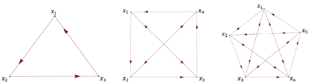
Refer to caption — Figure 1. Directed complete graphs

It is easy to see that

(5.1)

\operatorname{diam}\mathcal{K}_{n}=2,\quad\mathcal{H}_{x_{i}}=\overleftarrow{\mathcal{H}}_{x_{i}}=-\left(1+\cfrac{1}{2(n-2)}\right),\quad\Lambda=2+\cfrac{1}{n-2}

for all $n\geq 3$ and $i=1,\dots,n$ . The authors [15] have calculated the Ricci curvature of the edges of $\mathcal{K}_{n}$ as follows (see [15, Example 4.1]): (1) $\kappa(\mathcal{K}_{3})=3/2$ ; (2) if $n=4$ , then we have

\displaystyle\kappa(x_{1},x_{i})=\begin{cases}1&\text{if $i=2$},\\ \cfrac{3}{2}&\text{if $i=3$};\end{cases}

(3) if $n=5$ , then we have

\displaystyle\kappa(x_{1},x_{i})=\begin{cases}1&\text{if $i=2$},\\ \cfrac{7}{6}&\text{if $i=3$ or $4$};\end{cases}

(4) if $n\geq 6$ , then we have

\displaystyle\kappa(x_{1},x_{i})=\begin{cases}1&\text{if $i=2$ or $i\in\{4,\dots,n-2\}$},\\ 1+\cfrac{1}{2(n-2)}&\text{if $i=3$ or $n-1$}.\end{cases}

In particular,

(5.2)

K=\begin{cases}\cfrac{3}{2}&\text{if $n=3$},\\ 1&\text{if $n\geq 4$}.\end{cases}

By (5.1), (5.2), the equality (1.4) in holds on $\mathcal{K}_{n}$ if and only if $n=3$ . Actually, $\mathcal{K}_{n}$ is not spherically suspended for $n\geq 4$ although it is covered by minimal geodesics from $x_{1}$ to $x_{n}$ .

Remark 5.1.

It is remarkable that undirected (usual) complete graph with $3$ vertices does not have maximal diameter.

5.2. Directed triforce graphs

We next observe the unweighted directed triforce graph $\mathcal{T}$ (see Figure 2).

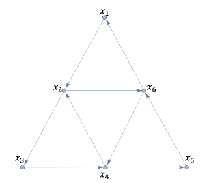
We verify that $\kappa(\mathcal{T})=3/4$ , and $\mathcal{T}$ has maximal diameter as follows: It is trivial that

(5.3)

\operatorname{diam}\mathcal{T}=4.

We calculate the asymptotic mean curvature. Since $\mathcal{T}$ is Eulerian, the formula (2.2) implies

(5.4)

\mathcal{P}(x_{1},z)=\begin{cases}\cfrac{1}{2}&\text{if $z=x_{2}$ or $x_{6}$},\\ 0&\text{otherwise},\end{cases}\quad\mathcal{P}(x_{2},z)=\begin{cases}\cfrac{1}{4}&\text{if $z=x_{1}$ or $x_{3}$ or $x_{4}$ or $x_{6}$},\\ 0&\text{otherwise},\end{cases}

for instance. From straightforward computations, it follows that

(5.5)

\mathcal{H}_{x_{i}}=\overleftarrow{\mathcal{H}}_{x_{i}}=-\frac{3}{2},\quad\Lambda=3

for all $i$ . Let us check that $\kappa(\mathcal{T})=3/4$ . To do so, by the symmetry, it is enough to calculate $\kappa(x_{1},x_{2}),\,\kappa(x_{2},x_{6})$ and $\kappa(x_{2},x_{3})$ . We here only present the calculation for $\kappa(x_{1},x_{2})$ , and the others are left to the reader. By (5.4),

\displaystyle\nu^{\varepsilon}_{x_{1}}(z)=\begin{cases}1-\varepsilon&\text{if $z=x$,}\\ \cfrac{\varepsilon}{2}&\text{if $z=x_{2}$ or $x_{6}$,}\\ 0&\text{otherwise},\end{cases}\quad\nu^{\varepsilon}_{x_{2}}(z)=\begin{cases}1-\varepsilon&\text{if $z=y$,}\\ \cfrac{\varepsilon}{4}&\text{if $z=x_{1}$ or $x_{3}$ or $x_{4}$ or $x_{6}$,}\\ 0&\text{otherwise}.\end{cases}

We define a coupling $\pi$ of $(\nu^{\varepsilon}_{x_{1}},\nu^{\varepsilon}_{x_{2}})$ by

\displaystyle\pi(z,w):=\begin{cases}1-\varepsilon-\cfrac{\varepsilon}{2}&\text{if $(z,w)=(x_{1},x_{2})$},\\ \cfrac{\varepsilon}{4}&\text{if $(z,w)=(x_{1},x_{1})$ or $(x_{1},x_{3})$ or $(x_{6},x_{4})$ or $(x_{6},x_{6})$},\\ 0&\text{otherwise}.\end{cases}

Then one can prove $W(\nu^{\varepsilon}_{x_{1}},\nu^{\varepsilon}_{x_{2}})\leq 1-3\varepsilon/4$ by (2.3), and hence $\kappa(x_{1},x_{2})\geq 3/4$ . To check the opposite inequality, we define a $1$ -Lipschitz function $f:V\to\mathbb{R}$ by

\displaystyle f(z):=\begin{cases}2&\text{if $z=x_{3}$},\\ 1&\text{if $z=x_{2}$},\\ -1&\text{if $z=x_{6}$},\\ 0&\text{otherwise}.\end{cases}

Applying Proposition 2.3 to the function $f$ , we obtain $\kappa(x_{1},x_{2})\leq 3/4$ . This proves $\kappa(x_{1},x_{2})=3/4$ . Notice that in the verification of $\kappa(x_{2},x_{6})=3/4$ , we use

	$\displaystyle\pi(z,w)$	$\displaystyle:=\begin{cases}1-\varepsilon-\cfrac{\varepsilon}{4}&\text{if $(z,w)=(x_{2},x_{6})$},\\ \cfrac{\varepsilon}{4}&\text{if $(z,w)=(x_{1},x_{1})$ or $(x_{2},x_{2})$ or $(x_{3},x_{5})$ or $(x_{4},x_{4})$ or $(x_{6},x_{6})$},\\ 0&\text{otherwise},\end{cases}$
	$\displaystyle f(z)$	$\displaystyle:=\begin{cases}2&\text{if $z=x_{5}$},\\ 1&\text{if $z=x_{4}$ or $x_{6}$},\\ 0&\text{otherwise}.\end{cases}$

Also, in the verification of $\kappa(x_{2},x_{3})=3/4$ ,

	$\displaystyle\pi(z,w)$	$\displaystyle:=\begin{cases}1-\varepsilon-\cfrac{\varepsilon}{2}&\text{if $(z,w)=(x_{2},x_{3})$},\\ \cfrac{\varepsilon}{4}&\text{if $(z,w)=(x_{1},x_{3})$ or $(x_{3},x_{3})$ or $(x_{4},x_{4})$ or $(x_{6},x_{4})$},\\ 0&\text{otherwise},\end{cases}$
	$\displaystyle f(z)$	$\displaystyle:=\begin{cases}2&\text{if $z=x_{4}$},\\ 1&\text{if $z=x_{3}$ or $x_{6}$},\\ 0&\text{otherwise}.\end{cases}$

Thus we arrive at

(5.6)

\kappa(\mathcal{T})=\frac{3}{4},\quad K=\frac{3}{4}.

Combining (5.3), (5.5) and (5.6), we conclude that $\mathcal{T}$ has maximal diameter.

Remark 5.2.

We consider the unweighted directed multi triforce graph (see Figure 3).

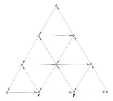
Then we see $\kappa(x,y)=0$ ; in particular, it does not have positive Ricci curvature.

5.3. Product and maximal diameter

We consider two simple, strongly connected, finite weighted directed graphs $(V,\mu)$ and $(V^{\prime},\mu^{\prime})$ , and also their $(\alpha,\beta)$ -weighted Cartesian product $(V,\mu)\square_{(\alpha,\beta)}(V^{\prime},\mu^{\prime})$ . Let us denote by $D,\,D^{\prime}$ and $D_{(\alpha,\beta)}$ the diameter of $(V,\mu),\,(V^{\prime},\mu^{\prime})$ and $(V,\mu)\square_{(\alpha,\beta)}(V^{\prime},\mu^{\prime})$ , respectively. We also denote by $\Lambda,\,\Lambda^{\prime}$ and $\Lambda_{(\alpha,\beta)}$ the value defined as (1.2) of $(V,\mu),\,(V^{\prime},\mu^{\prime})$ and $(V,\mu)\square_{(\alpha,\beta)}(V^{\prime},\mu^{\prime})$ , respectively. Furthermore, We denote by $K,\,K^{\prime}$ and $K_{(\alpha,\beta)}$ the value done by (1.1) of $(V,\mu),\,(V^{\prime},\mu^{\prime})$ and $(V,\mu)\square_{(\alpha,\beta)}(V^{\prime},\mu^{\prime})$ , respectively.

Lemma 5.3.

D_{(\alpha,\beta)}=D+D^{\prime},\quad\Lambda_{(\alpha,\beta)}=\frac{\beta}{\alpha+\beta}\Lambda+\frac{\alpha}{\alpha+\beta}\Lambda^{\prime},\quad K_{(\alpha,\beta)}=\min\left\{\frac{\beta}{\alpha+\beta}K,\frac{\alpha}{\alpha+\beta}K^{\prime}\right\}.

Proof.

The assertions for $D$ and $\Lambda$ are immediately derived from (3.4) and (3.5). For $K$ , Theorem 3.5 implies

	$\displaystyle K_{(\alpha,\beta)}$	$\displaystyle=\min\left\{\inf_{x\rightarrow y,\,x^{\prime}\in V^{\prime}}\kappa_{(\alpha,\beta)}((x,x^{\prime}),(y,x^{\prime})),\inf_{x\in V,\,x^{\prime}\rightarrow y^{\prime}}\kappa_{(\alpha,\beta)}((x,x^{\prime}),(x,y^{\prime}))\right\}$
		$\displaystyle=\min\left\{\frac{\beta}{\alpha+\beta}\inf_{x\rightarrow y}\kappa(x,y),\frac{\alpha}{\alpha+\beta}\inf_{x^{\prime}\rightarrow y^{\prime}}\kappa^{\prime}(x^{\prime},y^{\prime})\right\}=\min\left\{\frac{\beta}{\alpha+\beta}K,\frac{\alpha}{\alpha+\beta}K^{\prime}\right\}.$

This proves the lemma. $\Box$

The following claim together with the observation in Subsections 5.1 and 5.2 enables us to produce new directed graphs having maximal diameter:

Theorem 5.4.

We assume $K,K^{\prime}>0$ . Then the following are equivalent:

(1)

The equality (1.4) holds on $(V,\mu)$ and $(V^{\prime},\mu^{\prime})$ , and $\alpha D\Lambda^{\prime}=\beta D^{\prime}\Lambda$ ;
(2)

the equality (1.4) holds on $(V,\mu)\square_{(\alpha,\beta)}(V^{\prime},\mu^{\prime})$ .

Proof.

The implication from (1) to (2) is a direct consequence of Lemma 5.3. Let us prove the opposite direction. By virtue of Lemma 5.3, the assumption, and Theorem 1.1,

(5.7)

\frac{\displaystyle\frac{\beta}{\alpha+\beta}\Lambda+\frac{\alpha}{\alpha+\beta}\Lambda^{\prime}}{D+D^{\prime}}=\frac{\Lambda_{(\alpha,\beta)}}{D_{(\alpha,\beta)}}=K_{(\alpha,\beta)}\leq\frac{\beta}{\alpha+\beta}K\leq\frac{\beta}{\alpha+\beta}\frac{\Lambda}{D},

and hence $\alpha D\Lambda^{\prime}\leq\beta D^{\prime}\Lambda$ . Similarly,

(5.8)

\frac{\displaystyle\frac{\beta}{\alpha+\beta}\Lambda+\frac{\alpha}{\alpha+\beta}\Lambda^{\prime}}{D+D^{\prime}}=\frac{\Lambda_{(\alpha,\beta)}}{D_{(\alpha,\beta)}}=K_{(\alpha,\beta)}\leq\frac{\alpha}{\alpha+\beta}K^{\prime}\leq\frac{\alpha}{\alpha+\beta}\frac{\Lambda^{\prime}}{D^{\prime}},

and hence $\alpha D\Lambda^{\prime}\geq\beta D^{\prime}\Lambda$ . It follows that $\alpha D\Lambda^{\prime}=\beta D^{\prime}\Lambda$ . Furthermore, the inequalities in (5.7), (5.8) become equalities. Thus we conclude the desired assertion. $\Box$

Cushing et al. [7] have proved Theorem 5.4 for unweighted, undirected regular graphs (see [7, Theorem 3.2]).

Example 5.5.

For example, for $\alpha_{1},\dots,\alpha_{m}>0$ , the Cartesian product

\{(\mathcal{K}_{3}\square_{(\alpha_{1},\alpha_{1})}\mathcal{K}_{3})\square_{(\alpha_{2},2\alpha_{2})}\mathcal{K}_{3}\}\square_{(\alpha_{3},3\alpha_{3})}\cdots\square_{(\alpha_{m},m\alpha_{m})}\mathcal{K}_{3}

has maximal diameter, whose diameter is $2(m+1)$ , value defined as (1.2) is $3$ , and value defined as (1.1) is $3/2(m+1)$ .

Acknowledgements

The authors thank Professor Takashi Shioya for informing them of [12]. They are also grateful to Doctor Daisuke Kazukawa for his useful comments. The first named author was supported in part by JSPS KAKENHI (19K14532). The first and second named authors were supported in part by JSPS Grant-in-Aid for Scientific Research on Innovative Areas “Discrete Geometric Analysis for Materials Design” (17H06460). The third named author was supported in part by JSPS KAKENHI (19K23411).

References

[1] A. Adriani and A. G. Setti, Inner-Outer Curvatures, Ricci-Ollivier Curvature and Volume Growth of Graphs, preprint arXiv:2009.12814.
[2] F. Bauer, J. Jost and S. Liu, Ollivier-Ricci curvature and the spectrum of the normalized graph Laplace operator, Math. Res. Lett. 19 (2012), no. 6, 1185–1205.
[3] B. Benson, P. Ralli and P. Tetali, Volume growth, curvature, and Buser-type inequalities in graphs, Int. Math. Res. Not. IMRN, 2019, rnz305.
[4] D. P. Bourne, D. Cushing, S. Liu, F. Münch and N. Peyerimhoff, Ollivier-Ricci idleness functions of graphs, SIAM J. Discrete Math. 32 (2018), no. 2, 1408–1424.
[5] F. Chung, Laplacians and the Cheeger inequality for directed graphs, Ann. Comb. 9 (2005), no. 1, 1–19.
[6] F. Chung, The diameter and Laplacian eigenvalues of directed graphs, Electron. J. Combin. 13 (2006), no. 1, Note 4, 6 pp.
[7] D. Cushing, S. Kamtue, J.Koolen, S. Liu, F. F. Münch and N. Peyerimhoff, Rigidity of the Bonnet-Myers inequality for graphs with respect to Ollivier Ricci curvature, Adv. Math. 369 (2020), 107188.
[8] A. Grigor’yan, Introduction to Analysis on Graphs, University Lecture Series, 71. American Mathematical Society, Providence, RI, 2018.
[9] J. Jost and S. Liu, Ollivier’s Ricci curvature, local clustering and curvature-dimension inequalities on graphs, Discrete Comput. Geom. (2) 53 (2014), 300–322.
[10] J. H. Koolen, V. Moulton and D. Stevanović, The structure of spherical graphs, European J. Combin. 25 (2004), no. 2, 299–310.
[11] Y. Lin, L. Lu and S.-T. Yau, Ricci curvature of graphs, Tohoku Math. J. (2) 63 (2011), no. 4, 605–627.
[12] M. Matsumoto, Master thesis (Japanese), Mathematical Institute, Tohoku University, 2010.
[13] F. Münch and R. K. Wojciechowski, Ollivier Ricci curvature for general graph Laplacians: Heat equation, Laplacian comparison, non-explosion and diameter bounds, Adv. Math. 356 (2019), 106759, 45 pp.
[14] Y. Ollivier, Ricci curvature of Markov chains on metric spaces, J. Funct. Anal. 256 (2009), no. 3, 810–864.
[15] R. Ozawa, Y. Sakurai and T. Yamada, Geometric and spectral properties of directed graphs under a lower Ricci curvature bound, Calc. Var. Partial Differential Equations 59 (2020), no. 4, Paper No. 142, 39 pp.
[16] S.-H. Paeng, Volume and diameter of a graph and Ollivier’s Ricci curvature, European J. Combin. 33 (2012), no. 8, 1808–1819.
[17] C. Villani, Optimal Transport: Old and New, Springer-Verlag, Berlin, 2009.