Maximum $k$ -Plex Search: An Alternated Reduction-and-Bound Method

Shuohao Gao Harbin Institute of Technology, ShenzhenChina 200111201@stu.hit.edu.cn , Kaiqiang Yu Nanyang Technological UniversitySingapore kaiqiang002@e.ntu.edu.sg , Shengxin Liu Harbin Institute of Technology, ShenzhenChina sxliu@hit.edu.cn and Cheng Long Nanyang Technological UniversitySingapore c.long@ntu.edu.sg

(2018)

Abstract.

$k$ -plexes relax cliques by allowing each vertex to disconnect to at most $k$ vertices. Finding a maximum $k$ -plex in a graph is a fundamental operator in graph mining and has been receiving significant attention from various domains. The state-of-the-art algorithms all adopt the branch-reduction-and-bound (BRB) framework where a key step, called reduction-and-bound (RB), is used for narrowing down the search space. A common practice of RB in existing works is SeqRB, which sequentially conducts the reduction process followed by the bounding process once at a branch. However, these algorithms suffer from the efficiency issues. In this paper, we propose a new alternated reduction-and-bound method AltRB for conducting RB. AltRB first partitions a branch into two parts and then alternatively and iteratively conducts the reduction process and the bounding process at each part of a branch. With newly-designed reduction rules and bounding methods, AltRB is superior to SeqRB in effectively narrowing down the search space in both theory and practice. Further, to boost the performance of BRB algorithms, we develop efficient and effective pre-processing methods which reduce the size of the input graph and heuristically compute a large $k$ -plex as the lower bound. We conduct extensive experiments on 664 real and synthetic graphs. The experimental results show that our proposed algorithm kPEX with AltRB and novel pre-processing techniques runs up to two orders of magnitude faster and solves more instances than state-of-the-art algorithms.

^†^†copyright: acmlicensed^†^†journalyear: 2018^†^†doi: XXXXXXX.XXXXXXX^†^†conference: Make sure to enter the correct conference title from your rights confirmation emai; June 03–05, 2018; Woodstock, NY^†^†isbn: 978-1-4503-XXXX-X/18/06

1. Introduction

The graph model serves as a versatile tool for abstracting numerous real-world data which captures relationships between diverse entities in social networks, biological networks, publication networks, and so on. Cohesive subgraph mining is one of the central topics in graph analysis and data mining where the objective is to mine those dense or cohesive subgraphs that normally bring valuable insights for analysis (Lee et al., 2010; Chang and Qin, 2018; Huang et al., 2019; Fang et al., 2020, 2021). For example, cohesive subgraph mining has been used to detect a terrorist cell in social networks (Krebs, 2002), to identify protein complexes in biological networks (Zhang et al., 2014), and to find a group of research collaborators in publication networks (Guo et al., 2022).

The clique is arguably the most well-known cohesive subgraph where every pair of distinct vertices is connected by an edge. In the literature, the study of efficient algorithms for extracting the maximum clique or enumerating maximal cliques is extensive, e.g., (Carraghan and Pardalos, 1990; Pardalos and Xue, 1994; Tomita, 2017; Chang, 2019; Conte et al., 2016; Eppstein et al., 2013; Naudé, 2016; Tomita et al., 2006). Nevertheless, clique, being a tightly interconnected subgraph, is over-restrictive, which limits its practical usefulness. To circumvent this issue, relaxations of clique have been proposed and studied in the literature, such as $k$ -plex (Seidman and Foster, 1978), $k$ -core (Seidman, 1983), quasi-clique (Guo et al., 2020; Yu and Long, 2023a), and $k$ -defective clique (Chang, 2023; Dai et al., 2023a). In particular, $k$ -plex relaxes clique by allowing each vertex to disconnect to at most $k$ vertices (including the vertex itself). It is clear that 1-plex corresponds to clique. The research of cohesive subgraph mining in the context of $k$ -plex has recently attracted increasing interests (Xiao et al., 2017; Wang et al., 2023; Gao et al., 2018; Zhou et al., 2021; Jiang et al., 2021; Chang et al., 2022; Jiang et al., 2023; Dai et al., 2022b; Wang et al., 2022; Chang and Yao, 2024).

In this paper, we study the maximum $k$ -plex search problem which aims to search the $k$ -plex with the largest number of vertices in the given graph. It is well-known that the maximum $k$ -plex search problem is NP-hard for any fixed $k$ (Balasundaram et al., 2011). Thus, existing studies and ours focus on designing practically efficient algorithms.

Existing algorithms. The state-of-the-art algorithms all (conceptually) adopt the branch-reduction-and-bound (BRB) framework (Gao et al., 2018; Zhou et al., 2021; Jiang et al., 2021; Chang et al., 2022; Jiang et al., 2023; Wang et al., 2023; Chang and Yao, 2024). The idea is to recursively solve the problem instance (or branch) by solving the subproblem instances (or sub-branches) produced via a process of branching. A branch denoted by $(S,C)$ corresponds to a problem instance of finding the largest $k$ -plex from the subgraph (of the input graph) induced by vertex set $S\cup C$ , where the partial solution $S$ corresponds to a $k$ -plex and the candidate set $C$ corresponds to the set of vertices used to expand the partial solution. We refer the search space of a branch to the set of possible $k$ -plexes in the subgraph induced by $S\cup C$ . At each branch, a key step, named reduction-and-bound (RB), is performed for narrowing down the search space. We note that existing studies all follow a sequential framework, called SeqRB, for implementing the RB step. Specifically, SeqRB sequentially conducts two processes once: 1) the reduction process shrinks the candidate set $C$ by removing some unpromising vertices that cannot appear in the largest $k$ -plex; and 2) the bounding process computes the upper bound of the size of the largest $k$ -plex in the branch refined by the first step, which is used for pruning unnecessary branches (i.e., with the upper bound no larger than the largest $k$ -plex seen so far). The rationale behind is that with some vertices being removed by the reduction process, the bounding process may obtain a smaller upper bound so as to prune more branches.

Existing studies focus solely on sharpening the reduction rules and upper bound computation methods used in SeqRB while devoting little effort to improving the whole RB framework. We observe that, in SeqRB, the reduction process benefits the bounding process, but not the other way; and thus they are sequentially conducted only once. One interesting question is that: Can we design a new RB framework where the reduction process and the bounding process can benefit each other?

We remark that some recent studies (Zhou et al., 2021; Chang et al., 2022; Jiang et al., 2023; Wang et al., 2023; Chang and Yao, 2024) boost the practical performance of BRB algorithms by devising various pre-processing techniques. These techniques include 1) graph reduction algorithms (Zhou et al., 2021; Chang et al., 2022) for reducing the size of the input graph (among which the best one is CTCP (Chang et al., 2022)); and 2) heuristic algorithms (Zhou et al., 2021; Chang et al., 2022; Chang and Yao, 2024) for computing an initial large $k$ -plex used for the above-mentioned reduction algorithms (among which the best ones are kPlex-Degen (Chang et al., 2022) and EGo-Degen (Chang and Yao, 2024)).

Our new methods. In this paper, we first propose a new framework, called alternated reduction-and-bound (AltRB), for conducting the RB step at a branch $(S,C)$ . AltRB differs from SeqRB mainly in the way of conducting the reduction process and the bounding process. Specifically, AltRB first partitions a branch into two parts (i.e., $S=S_{L}\cup S_{R}$ and $C=C_{L}\cup C_{R}$ ). With newly-designed reduction rules and upper bound computation methods on each part, the bounding process on one part will benefit the reduction process on the other (note that the reduction process still benefits the bounding process on the same part, which is the same as SeqRB). Thus, AltRB alternatively and iteratively conducts the reduction process and the bounding process at each part of a branch (e.g., bounding on $S_{L}\cup C_{L}$ $\rightarrow$ reduction on $S_{R}\cup C_{R}$ $\rightarrow$ bounding on $S_{R}\cup C_{R}$ $\rightarrow$ reduction on $S_{L}\cup C_{L}$ $\rightarrow$ …). In this manner, the bounding process and the reduction process could mutually benefit from each other. We show that AltRB is superior to SeqRB in narrowing down the search space in both theory (as will be shown in Equation (9)) and practice (as will be shown in Table 4). We further design efficient pre-processing techniques for boosting the practical performance of BRB algorithms: 1) a new method CF-CTCP, which differs with CTCP in the way of conducting different reductions at each iteration, and 2) a heuristic algorithm KPHeuris that iteratively compute a large initial maximal $k$ -plex.

With all the above newly-designed techniques, we develop a new BRB algorithm called kPEX, which runs up to two orders of magnitude faster and solves more instances than state-of-the-art algorithms kPlexT (Chang and Yao, 2024), kPlexS (Chang et al., 2022), KPLEX (Wang et al., 2023), and DiseMKP (Jiang et al., 2023).

Our contributions. Our main contributions are as follows.

•

We propose a new BRB algorithm called kPEX, which incorporates the proposed alternated reduction-and-bound method AltRB (Section 3). With our newly devised reduction rules and bounding methods, AltRB is superior to SeqRB in narrowing down the search space (Section 4).
•

We design efficient pre-processing techniques for boosting the performance of BRB algorithms, namely a new method CF-CTCP for reducing the size of the input graph and a heuristic KPHeuris for computing a large initial $k$ -plex (Section 5).
•

We conduct extensive experiments on 664 real and synthetic graphs to verify the effectiveness and efficiency of our algorithms. Compared with the state-of-the-art algorithms, our kPEX 1) solves most number of graph instances within the time limit and 2) runs up to two orders of magnitude faster than existing algorithms (Section 6).

2. Preliminaries

Let $G=(V,E)$ be a simple graph with $|V|=n$ vertices and $|E|=m$ edges. A vertex $v$ is said to be a neighbor of (or adjacent to) vertex $u$ if there is an edge between $u$ and $v$ , i.e., $(u,v)\in E$ . Denote by $N_{G}(u)=\{v\in V~|~(u,v)\in E\}$ and $d_{G}(u)=|N_{G}(u)|$ the neighbor set and the degree of the vertex $u$ in $G$ , respectively. Given a vertex subset $S\subseteq V$ , we use $G[S]$ to denote the subgraph induced by $S$ , i.e., $G[S]=(S,\{(u,v)\in E~|~u,v\in S\})$ , and use $N_{G}(u,S)$ (resp. $\overline{N}_{G}(u,S)$ ) to denote sets of neighbors (resp. non-neighbors that include $u$ itself) of $u$ in $G[S]$ . We omit the subscript $G$ when the context is clear. Given a graph $g$ , we use $V(g)$ and $E(g)$ to denote the sets of vertices and edges in $g$ , respectively.

In this paper, we focus on the cohesive subgraph of $k$ -plex.

Definition 2.1 ( $k$ -plex (Seidman and Foster, 1978)).

Given a positive integer $k$ , a graph $g$ is said to be a $k$ -plex if $d_{g}(u)\geq|V(g)|-k$ for each vertex $u\in V(g)$ .

Obviously, a 1-plex is a clique where each two vertices are adjacent. Note also that $k$ -plex has the hereditary property, i.e., any induced subgraph of a $k$ -plex is also a $k$ -plex (Seidman and Foster, 1978).

Problem statement. Given a graph $G=(V,E)$ and an integer $k\geq 2$ , the maximum $k$ -plex search problem aims to find the largest $k$ -plex $G[S]$ with $|S|\geq 2k-1$ in $G$ .

Following the previous studies (Chang et al., 2022; Wang et al., 2023), we focus on finding $k$ -plexes with at least $2k-1$ vertices for the following considerations. First, the value of $k$ is usually small in real applications, e.g., $k\leq 6$ in (Xiao et al., 2017; Gao et al., 2018; Zhou et al., 2021; Jiang et al., 2021). Hence, a $k$ -plex with at most $2k-2$ vertices is less informative in practice. Second, a $k$ -plex with at least $2k-1$ vertices has the diameter of at most 2 (Zhou et al., 2021), which is more cohesive.

We next introduce some useful concepts used in this paper.

$k$ -core/ $k$ -truss. We review useful cohesive subgraph definitions.

Definition 2.2.

Given a positive integer $k$ , a graph $g$ is said to be

•

a $k$ -core if $d_{g}(u)\geq k$ for each vertex $u\in V(g)$ (Seidman, 1983);
•

a $k$ -truss if each edge $(u,v)\in E(g)$ belongs to at least $k-2$ triangles, i.e., $|N_{g}(u)\cap N_{g}(v)|\geq k-2$ for each edge $(u,v)\in E(g)$ (Cohen, 2008).

Clearly, a $k$ -core $g$ is a $\big{(}|V(g)|-k\big{)}$ -plex and a $k$ -truss $g^{\prime}$ is a $\big{(}|V(g^{\prime})|-k+1\big{)}$ -plex.

Degeneracy order. The sequence of vertices $v_{1},v_{2},...,v_{n}$ in $G=(V,E)$ is called the degeneracy order of $G$ if $v_{i}$ has the minimum degree in $G[\{v_{i},v_{i+1},...,v_{n}\}]$ for each $v_{i}$ in $V$ (Batagelj and Zaveršnik, 2003). Further, the degeneracy of $G$ , denoted by $\delta(G)$ (or $\delta$ if the context is clear), is defined as the smallest number such that every induced subgraph of $G$ has a vertex of degree at most $\delta(G)$ . In other words, $G$ does not have an induced subgraph that is a $(\delta+1)$ -core. The degeneracy order and the value of $\delta$ can be obtained by iteratively peeling the vertex with minimum degree in the current induced subgraph with time complexity of $O(m)$ (Batagelj and Zaveršnik, 2003). Also, it is known that $\delta\leq\sqrt{n+2m}$ (Chang, 2019).

3. The Framework of kPEX

Our algorithm, named kPEX, follows the branch-reduction-and-bound (BRB) framework which is (conceptually) adopted by existing algorithms (Gao et al., 2018; Zhou et al., 2021; Jiang et al., 2021; Chang et al., 2022; Jiang et al., 2023; Wang et al., 2023; Chang and Yao, 2024). The idea is to recursively partition the current problem instance of finding the largest $k$ -plex into two subproblem instances via a process of branching. Specifically, a problem instance (or branch) is denoted by $(G,S,C)$ (or, simply $(S,C)$ when the context is clear) where the partial solution $S$ induces a $k$ -plex (i.e., $G[S]$ ) and the candidate set $C$ is a set of vertices that will be used to expand $S$ . Solving the branch $(S,C)$ refers to finding the largest $k$ -plex $G[H]$ in the branch; a $k$ -plex is in the branch $(S,C)$ if and only if $S\subseteq H\subseteq S\cup C$ . To solve a branch $(S,C)$ , it recursively solves two sub-branches formed based on a branching vertex $v$ selected from $C$ : one branch $(S\cup\{v\},C\setminus\{v\})$ includes $v$ to the partial solution $S$ (which finds the largest $k$ -plex containing $v$ in $(S,C)$ ), and the other $(S,C\setminus\{v\})$ discards $v$ from the candidate set $C$ (which finds the largest $k$ -plex excluding $v$ in $(S,C)$ ). Clearly, solving two formed sub-branches solves branch $(S,C)$ , and solving the branch $(\emptyset,V)$ finds the largest $k$ -plex in $G$ .

Input: A graph

G=(V,E)

and an integer

k

Output: The largest

k

-plex

G[S^{*}]

/* Stage-I.1: Heuristic&Preprocessing (Sec. 5) */

S^{*}\leftarrow

a large

k

-plex via a heuristic process KPHeuris;

G\leftarrow

apply reduction method CF-CTCP to reduce

G

;

/* Stage-I.2: Divide-and-conquer framework */

3 while $V(G)\neq\emptyset$ do

v\leftarrow

the vertex with the minimum degree in

G

;

g\leftarrow

the subgraph of

G

induced by

N^{\leq 2}(v)

;

/* Stage-II:branch-reduction-bound (Sec. 4) */

6 BRB_Rec

(g,\{v\},V(g)\setminus\{v\},k)

;

G\leftarrow

apply reduction method CF-CTCP to reduce

G

;

9return

G[S^{*}]

;

11 Procedure BRB_Rec

(G,S,C,k)

C^{\star},UB^{\star}\leftarrow

AltRB

(G,S,C,k)

;

13 if $UB^{\star}\leq|S^{*}|$ then return;

14 if $S\!\cup\!C^{\star}$ is a $k$ -plex then update

S^{*}

S\!\cup\!C^{\star}

and return;

v^{*}\leftarrow

a branching vertex selected from

C^{\star}

;

16 BRB_Rec

(G,S\cup\{v^{*}\},C^{\star}\setminus\{v^{*}\},k)

;

17 BRB_Rec

(G,S,C^{\star}\setminus\{v^{*}\},k)

;

Algorithm 1 Our framework: kPEX

Our kPEX adopts a similar framework in (Chang et al., 2022), which is summarized in Algorithm 1 and involves two stages. Stage-I first includes, in Stage-I.1, a heuristic method called KPHeuris for computing a large $k$ -plex $G[S^{*}]$ (maintained globally as the largest $k$ -plex seen so far), which will be used to narrow down the search space (Line 1), and a reduction method called CF-CTCP for reducing the input graph $G$ by removing unpromising vertices/edges that will not appear in any $k$ -plex larger than $|S^{*}|$ (Line 2). Besides, kPEX employs a widely-used divide-and-conquer strategy in Stage-I.2, which divides the problem of finding the largest $k$ -plex in $G$ into several sub-problems (Lines 3-7). Each sub-problem corresponds to a vertex $v$ in $G$ and aims to find the largest $k$ -plex that (1) includes vertex $v$ and (2) is in a subgraph of $G$ induced by $v$ ’s two-hop neighbours $N^{\leq 2}(v)$ , i.e., the set of vertices that have distance at most 2 from $v$ (note that a $k$ -plex with at least $2k-1$ vertices has the diameter of at most 2 (Zhou et al., 2021) and thus the largest $k$ -plex containing $v$ is a subset of $N^{\leq 2}(v)$ ). Clearly, the largest $k$ -plex in $G$ is the largest one among those returned by all sub-problems. Stage-II corresponds to the recursive process of solving a branch (Lines 9-15). Specifically, BRB_Rec recursively branches as discussed above (Lines 13-15). Besides, BRB_Rec conducts the newly proposed alternated reduction-and-bound process (AltRB) on a branch $(S,C)$ for narrowing down the search space (Line 10). Specifically, it refines $C$ to $C^{\star}$ by removing some unpromising vertices and computes an upper bound $UB^{\star}$ of (the size of) the largest $k$ -plex in $(S,C)$ for terminating the branch. Finally, we can terminate the branch when (1) $UB^{\star}\leq|S^{*}|$ since no larger $k$ -plex is in the branch and (2) $S\cup C^{\star}$ is a $k$ -plex since $G[S\cup C^{\star}]$ is the largest $k$ -plex in the branch.

Novelty. Our framework differs from the state-of-the-art one (Chang et al., 2022) in the following aspects. First, in Stage-II, kPEX is based on the newly proposed AltRB for narrowing down the search space. Recall that existing methods conduct the reduction-and-bound (RB) process using a sequential method called SeqRB at Line 10 instead. We will show that AltRB performs better than SeqRB in Section 4. Specifically, it refines $C$ to a smaller set $C^{\star}$ (i.e., $|C^{\star}|\leq|C|$ ) and obtains a tighter upper bound $UB^{\star}$ (i.e., $UB^{\star}\leq UB$ ). Second, in Stage-I.1, kPEX employs the novel KPHeuris and CF-CTCP which are more effective and efficient than existing competitors in Section 5.

4. our reduction&bound method: AltRB

4.1. An Alternated Reduction-and-Bound Method

Recall that existing algorithms conduct the reduction-and-bound (RB) step using the sequential method SeqRB on a branch $B=(S,C)$ for narrowing down the search space. Specifically, SeqRB has two sequential procedures: 1) the reduction process refines the candidate set $C$ to $C^{\prime}$ based on $|S^{*}|$ (i.e., the lower bound of the branch), i.e., removing from $C$ those vertices that cannot appear in a $k$ -plex larger than $|S^{*}|$ ; and 2) the bounding process obtains the upper bound of the largest $k$ -plex in the refined branch $(S,C^{\prime})$ , i.e., the upper bound of the branch denoted by $UB(S,C^{\prime})$ . In this paper, we propose a new alternated reduction-and-bound method, called AltRB, which is based on a binary partition of a branch $B=(S,C)$ as below.

(1)

S=S_{L}\cup S_{R},\ \ C=C_{L}\cup C_{R}.

Let $G[H]$ be a $k$ -plex in the branch $B$ such that $G[H]$ is larger than the largest $k$ -plex $G[S^{*}]$ seen so far, i.e., $|H|\geq|S^{*}|+1$ (note that other $k$ -plexes have the size at most $|S^{*}|$ and thus can be ignored during the exploration of the branch). Based on the above partition, a $k$ -plex $G[H]$ in $B$ can be divided into three parts as below.

(2)

H=S\cup(C_{L}\cap H)\cup(C_{R}\cap H).

We denote by $LB_{L}$ and $UB_{L}$ (resp. $LB_{R}$ and $UB_{R}$ ) the lower and upper bounds of the size of $C_{L}\cap H$ (resp. $C_{R}\cap H$ ), respectively. Formally, we have

(3)

\displaystyle|C_{L}\cap H|\leq UB_{L},\ |C_{R}\cap H|\leq UB_{R}.

Besides, we have the following lemma on the above partition.

Lemma 4.1.

Given a branch $(S,C)$ with a partition, we have

(4)

|C_{L}\cap H|\geq(|S^{*}|+1)-|S|-UB_{R},\ |C_{R}\cap H|\geq(|S^{*}|+1)-|S|-UB_{L}.

Proof.

This can be easily verified since otherwise if $|C_{L}\cap H|<(|S^{*}|+1)-|S|-UB_{R}$ , we have $|H|=|S|+|C_{L}\cap H|+|C_{R}\cap H|<|S|+(|S^{*}|+1)-|S|-UB_{R}+UB_{R}=|S^{*}|+1$ , which contradicts with $|H|\geq|S^{*}|+1$ . A similar contradiction can be derived for the other case $|C_{R}\cap H|<(|S^{*}|+1)-|S|-UB_{L}$ . ∎

Based on Lemma 4.1, we define $LB_{L}$ and $LB_{R}$ as follows.

(5)

(|S^{*}|+1)-|S|-UB_{R}\leq LB_{L}\leq|C_{L}\cap H|

(6)

(|S^{*}|+1)-|S|-UB_{L}\leq LB_{R}\leq|C_{R}\cap H|

Input: A graph

G=(V,E)

, a branch

(S,C)

and an integer

k

Output: Refined candidate set

C^{\star}

and upper bound

UB^{\star}

S_{L},S_{R},C_{L},C_{R}\leftarrow

Partition

(G,S,C,k)

;

UB_{L}\leftarrow|C_{L}|

LB_{L}\leftarrow 0

;

3 while $UB_{L}$ is not equal to ComputeUB $(S_{L},C_{L})$ do

UB_{L}\leftarrow

ComputeUB

(S_{L},C_{L})

;

LB_{R}\leftarrow(|S^{*}|+1)-|S|-UB_{L}

;

C_{R}\leftarrow

RR1&RR2 on

C_{R}

;

UB_{R}\leftarrow

ComputeUB

(S_{R},C_{R})

;

LB_{L}\leftarrow(|S^{*}|+1)-|S|-UB_{R}

;

C_{L}\leftarrow

RR1&RR2 on

C_{L}

;

9return

C^{\star}\leftarrow C_{L}\cup C_{R}

and

UB^{\star}\leftarrow|S|+UB_{L}+UB_{R}

;

Algorithm 2 Alternated reduction-and-bound: AltRB

We note that Lemma 4.1 and Equations (5) and (6) indicate the relation between the lower bound of one part and the upper bound of the other, which enables AltRB. We summarize AltRB in Algorithm 2, which iteratively and alternatively conducts the reduction-and-bound step on the two partitions obtained via Partition (Line 1). Specifically, after initializing $UB_{L}$ and $LB_{L}$ in Line 2, AltRB involves the following steps (the details of the two procedures Partition and ComputeUB are provided in Section 4.2).

•

Step 1 (Bound on $C_{L}$ ). Compute the upper bound for $C_{L}$ (i.e., $UB_{L}$ ) via a procedure ComputeUB (Line 4).
•

Step 2 (Reduction on $C_{R}$ ). Update the lower bound for $C_{R}$ (i.e., $LB_{R}$ ) by $(|S^{*}|+1)-|S|-UB_{L}$ according to Lemma 4.1 and then refine $C_{R}$ based on the updated bounds via reduction rules RR1 and RR2 (Line 5).
•

Step 3 (Bound on $C_{R}$ ). Compute the upper bound for the refined $C_{R}$ (i.e., $UB_{R}$ ) via a procedure ComputeUB (Line 6).
•

Step 4 (Reduction on $C_{L}$ ). Update the lower bound for $C_{L}$ (i.e., $LB_{L}$ ) by $(|S^{*}|+1)-|S|-UB_{R}$ according to Lemma 4.1 and then refine $C_{L}$ based on the updated bounds via reduction rules RR1 and RR2 (Line 7).

Finally, we repeat Steps 1-4 until $UB_{L}$ remains unchanged (Line 3). We remark that once tighter upper bounds are obtained at Step 1 and Step 3, tighter lower bounds can be derived via Lemma 4.1 at Step 2 and Step 4 which will be used to boost the performance of RR1 and RR2. Below find the details of reduction rules.

RR1.

Given a branch $(S,C)$ with $LB_{L}$ and $LB_{R}$ , 1) for a vertex $v$ in $C_{L}$ , we remove $v$ from $C$ if $|N(v,S\cup C_{L})|<LB_{L}+|S|-k$ or $|N(v,S\cup C_{R})|<LB_{R}+|S|-k+1$ ; and 2) for a vertex $v$ in $C_{R}$ , we remove $v$ from $C$ if $|N(v,S\cup C_{L})|<LB_{L}+|S|-k+1$ or $|N(v,S\cup C_{R})|<LB_{R}+|S|-k$ .
RR2.

Given a branch $(S,C)$ with $UB_{L}$ and $UB_{R}$ , 1) if $UB_{L}+UB_{R}+|S|=|S^{*}|+1$ and $UB_{L}=|C_{L}|$ , we move all vertices in $C_{L}$ from $C$ to $S$ if $G[S\cup C_{L}]$ is a $k$ -plex; otherwise, i.e., it is not a $k$ -plex, we terminate the branch $(S,C)$ ; 2) if $UB_{L}+UB_{R}+|S|=|S^{*}|+1$ and $UB_{R}=|C_{R}|$ , we move all vertices in $C_{R}$ from $C$ to $S$ if $G[S\cup C_{R}]$ is a $k$ -plex; otherwise, i.e., it is not a $k$ -plex, we terminate the branch $(S,C)$ .

Benefits. Before proving the correctness, we show that AltRB better narrows down the search space than the existing SeqRB. The rationale behind is based on the following observations. First, at Step 2 and Step 4, RR1, and RR2 (which are based on $UB_{L}$ , $UB_{R}$ , $LB_{L}$ and $LB_{R}$ ) will remove from $C$ more vertices when the lower bounds $LB_{L}$ and $LB_{R}$ become larger and/or the upper bounds $UB_{L}$ and $UB_{R}$ become smaller; Second, at Step 1 and Step 3, with some vertices being removed from $C_{L}$ and $C_{R}$ , smaller upper bound $UB_{L}$ and $UB_{R}$ can be derived via ComupteUB (details refer to Section 4.2), and larger lower bounds $LB_{L}$ and $LB_{R}$ can also be obtained via Lemma 4.1; Third, as AltRB iteratively proceeds, the bounding process and the reduction process will benefit each other (since the former will derive smaller upper bounds and larger lower bounds after the latter while the latter will remove more vertices from $C$ after the former). In contrast, SeqRB cannot be conducted iteratively since (1) its reduction rules are only based on $|S^{*}|$ , which will not be changed after SeqRB and (2) thus repeating it multiple times cannot result in either a smaller candidate set $C$ or a smaller upper bound. We remark that the refined set $C^{\star}$ and the upper bound $UB^{\star}$ obtained by AltRB is potentially smaller than those obtained by SeqRB (which will be proved in Section 4.2). Thus, with the proposed AltRB, our algorithm kPEX runs up to two orders of magnitude faster than the state-of-the-arts, as verified in our experiments.

Correctness. We then show the correctness of AltRB. Note that AltRB admits an arbitrary partition on $(S,C)$ and any possible procedure for computing $UB_{L}$ and $UB_{R}$ that satisfy Equation (3).

The correctness of RR1 can be proved by contradiction. Consider a $k$ -plex $G[H]$ in branch $B$ with $|H|\geq|S^{*}|+1$ . Note that if such a $k$ -plex does not exist, RR1 is obviously correct since all $k$ -plexes in branch $B$ are no larger than $|S^{*}|$ and thus branch $B$ can be terminated. In general, there are two cases. First, assume that $G[H]$ contains a vertex $v$ in $C_{L}$ such that $|N(v,S\cup C_{L})|<LB_{L}+|S|-k$ . We get the contradiction by showing that $v$ has more than $k$ non-neighbours in $H$ and thus $G[H]$ is not a $k$ -plex since $|N(v,H)|=|N(v,H\cap(S\cup C_{L}))|+|N(v,H\cap C_{R})|\leq(LB_{L}+|S|-k-1)+|H\cap C_{R}|\leq(|S|+|H\cap C_{R}|+|H\cap C_{L}|)-(k+1)=|H|-(k+1)$ . Second, assume that $G[H]$ contains a vertex $v$ in $C_{L}$ such that $|N(v,S\cup C_{R})|<LB_{R}+|S|-k+1$ . Similarly, we derive the contradiction by showing that $v$ has more than $k$ non-neighbours in $H$ and thus $G[H]$ is not a $k$ -plex since $|N(v,H)|=|N(v,H\cap(S\cup C_{R}))|+|N(v,H\cap C_{L})|\leq(LB_{R}+|S|-k)+(|H\cap C_{L}|-1)\leq(|S|+|H\cap C_{R}|+|H\cap C_{L}|)-(k+1)=|H|-(k+1)$ (note that $|N(v,H\cap C_{L})|\leq|H\cap C_{L}|-1$ since $v$ is in $C_{L}$ and is not adjacent to itself). Symmetrically, we can prove the correctness for the reduction rules on $C_{R}$ .

The correctness of RR2 is easy to verify. Consider a branch $(S,C)$ with $UB_{L}+UB_{R}+|S|=|S^{*}|+1$ and $UB_{L}=|C_{L}|$ , and a $k$ -plex $G[H]$ in $(S,C)$ with $|H|\geq|S^{*}|+1$ (note that if such a $k$ -plex does not exist, RR2 is obviously correct on this branch). We note that $G[H]$ must contain all vertices in $C_{L}$ , i.e., $C_{L}\subseteq H$ , since otherwise $|H|=|H\cap S|+|H\cap C_{L}|+|H\cap C_{R}|\leq|S|+(|C_{L}|-1)+|H\cap C_{R}|\leq|S|+UB_{L}+UB_{R}-1=|S^{*}|$ . Therefore, $G[S\cup C_{L}]$ must be a $k$ -plex due to the hereditary property; otherwise, such a $k$ -plex cannot exist in $(S,C)$ and we can terminate the branch.

The correctness of AltRB can then be easily verified.

4.2. Upper Bound Computation and Greedy Partition Strategy

In this part, we first introduce the method ComputeUB used at Step 1 and Step 3 for obtaining $UB_{L}$ and $UB_{R}$ in Section 4.1. To boost the performance of ComputeUB as well as the reduction rules on $C_{L}$ and $C_{R}$ , we then propose a greedy strategy Partition for partitioning $C$ (resp. $S$ ) into $C_{L}$ and $C_{R}$ (resp. $S_{L}$ and $S_{R}$ ). Finally, with all carefully-designed techniques above, we show that the resulted upper bound $UB^{\star}$ will be potentially smaller than the existing one $UB$ .

Upper bound computation. We adapt an existing upper bound computation (Jiang et al., 2023), which we call ComputeUB, for obtaining $UB_{L}$ and $UB_{R}$ . Note that it can handle an arbitrary partition on a branch $(S,C)$ . Consider Step 1 for computing $UB_{L}$ . ComputeUB $(S_{L},C_{L})$ first iteratively partitions $C_{L}$ into $(|S_{L}|+1)$ disjoint subsets. The $i$ -th ( $1\leq i\leq|S_{L}|$ ) subset $\Pi_{i}(S_{L},C_{L})$ contains all non-neighbours of a vertex $u_{i}\in S_{L}$ in $C_{L}-\{\Pi_{1}(S_{L},C_{L}),...,\Pi_{i-1}(S_{L},C_{L})\}$ , formally,

(7)

\Pi_{i}(S_{L},C_{L})=\overline{N}(u_{i},C_{L}^{i}),\ C_{L}^{i}=C_{L}-\cup_{j=1}^{i-1}\Pi_{j}(S_{L},C_{L}),

where $u_{i}$ is the vertex in $S_{L}\setminus\{u_{1},u_{2},...,u_{i-1}\}$ with the largest ratio of $|\overline{N}(u_{i},C_{L}^{i})|/(k-|\overline{N}(u_{i},S)|)$ . Note that the strategy of selecting $u_{i}$ from $S_{L}$ has been shown to boost the practical performance of ComputeUB (details refer to (Jiang et al., 2023)). Besides, we have $\Pi_{0}(S_{L},C_{L})=C_{L}-\{\Pi_{1}(S_{L},C_{L}),...,\Pi_{|S_{L}|}(S_{L},C_{L})\}$ . Thus, vertices in $\Pi_{i}(S_{L},C_{L})$ ( $1\leq i\leq|S_{L}|$ ) are the non-neighbours of $u_{i}$ in $C_{L}$ , and vertices in $\Pi_{0}(S_{L},C_{L})$ are common neighbours of vertices in $S_{L}$ . The key observation is that for a $k$ -plex $G[H]$ in the branch, $C_{L}\cap H$ contains at most $\min\{|\Pi_{i}(S_{L},C_{L})|,k-|\overline{N}(u_{i},S)|\}$ vertices from $\Pi_{i}(S_{L},C_{L})$ for $1\leq i\leq|S_{L}|$ since otherwise $u_{i}$ (in $H$ ) will have more than $k$ non-neighbours in $G[H]$ and thus $G[H]$ is not a $k$ -plex. Thus, the upper bound $UB_{L}$ returned by ComputeUB $(S_{L},C_{L})$ gives as below:

(8)

|\Pi_{0}(S_{L},C_{L})|+\sum_{i=1}^{|S_{L}|}\min\{|\Pi_{i}(S_{L},C_{L})|,k-|\overline{N}(u_{i},S)|\}.

We note that with some vertices being removed from $C_{L}$ during AltRB, $\Pi_{i}(S_{L},C_{L})$ will get smaller and thus a smaller upper bound can be derived. Similarly, we can obtain $UB_{R}$ by ComputeUB $(S_{R},C_{R})$ . Besides, we remark that the state-of-the-art upper bound of $k$ -plex in the branch $(S,C)$ (used in SeqRB) is $|S|$ +ComputeUB $(S,C)$ (Jiang et al., 2023).

Greedy partition. Consider the upper bound computation at $C_{L}$ , i.e., Equation (8). We observe that all vertices in $\Pi_{0}(S_{L},C_{L})$ contributes to the upper bound ComputeUB $(S_{L},C_{L})$ since each of them is adjacent to all vertices in $S_{L}$ and thus they could appear in a $k$ -plex in branch $(S,C)$ . The similar observation can be derived on other subsets $\Pi_{i}(S_{L},C_{L})$ such that $|\overline{N}(u_{i},C_{L}^{i})|\leq k-|\overline{N}(u_{i},S)|$ and $1\leq i\leq|S_{L}|$ (note that there are fewer missing edges between $S_{L}$ and those subsets). Therefore, the adapted upper bound computation performs worse on those subsets.

Motivated by the above observation, we propose to divide $S$ and $C$ into the one ( $S_{L}$ and $C_{L}$ ) with more missing edges and the other ( $S_{R}$ and $C_{R}$ ) with fewer missing edges. We summarize the proposed strategy in Algorithm 3. Specifically, we iteratively remove from $S$ to $S_{L}$ (resp. from $C$ to $C_{L}$ ) the vertex $v$ with the greatest value of $|\overline{N}(v,C)|/(k-|\overline{N}(v,S)|)$ (resp. the set of $v$ ’s non-neighbours in $C$ , i.e., $\overline{N}(v,C)$ ) until the greatest value of $|\overline{N}(v,C)|/(k-|\overline{N}(v,S)|)$ is not greater than 1 or $S$ becomes empty (Lines 2-6). Then, all remaining vertices in $S$ and $C$ will be removed to $S_{R}$ and $C_{R}$ (Line 7). We observe that (1) ComputeUB $(S_{L},C_{L})$ will return a tighter bound since $|\overline{N}(u_{i},C_{L}^{i})|>k-|\overline{N}(u_{i},S)|$ holds for $1\leq i\leq|S_{L}|$ and $\Pi_{0}(S_{L},C_{L})=\emptyset$ , and (2) ComputeUB $(S_{R},C_{R})$ is always equal to $|C_{R}|$ .

Consider a branch $(S,C)$ (which has been refined by SeqRB) with the upper bound $UB=|S|$ +ComputeUB $(S,C)$ . With the proposed techniques, AltRB will further narrow down the search space of $(S,C)$ by the following observation.

(9)

UB^{\star}\leq UB\ \text{and}\ |C^{\star}|\leq|C|.

We note that $|C^{\star}|\leq|C|$ is obvious since some vertices in $C$ could be removed via RR1 and RR2. Besides, $UB^{\star}\leq UB$ holds since (1) ComputeUB $(S,C)=$ ComputeUB $(S_{L},C_{L})+$ ComputeUB $(S_{R},C_{R})$ before AltRB (which can be verified based on the definitions) and (2) as AltRB proceeds, $C_{L}$ and $C_{R}$ are refined via RR1 and RR2, and thus ComputeUB $(S_{L},C_{L})$ and ComputeUB $(S_{R},C_{R})$ get smaller.

Benefits of greedy partition. Compared with a random partition, the greedy partition in Algorithm 3 has the following advantageous properties. (1) A tight upper bound of $C_{L}$ leads to a larger $LB_{R}$ , which enhances the effectiveness of RR1. (2) $UB_{R}=|C_{R}|$ is always satisfied, which means that RR2 is applicable as long as $UB_{L}+UB_{R}+|S|=|S^{*}|+1$ . In other words, the conditions for RR2 are more relaxed. Moreover, computing $UB_{R}$ as $|C_{R}|$ is easy to implement and requires less computation.

Input: Branch

(S,C)

, a graph

G=(V,E)

, and an integer

k

Output: The greedy partition

S_{L}

S_{R}

C_{L}

and

C_{R}

S_{L}\leftarrow\emptyset

S_{R}\leftarrow\emptyset

C_{L}\leftarrow\emptyset

C_{R}\leftarrow\emptyset

;

2 while $S\neq\emptyset$ do

v^{*}\leftarrow\arg\max_{v\in S}|\overline{N}(v,C)|/(k-|\overline{N}(v,S)|)

;

4 if $|\overline{N}(v^{*},C)|/(k-|\overline{N}(v^{*},S)|)\leq 1$ then break;

S_{L}\leftarrow S_{L}\cup\{v^{*}\}

C_{L}\leftarrow C_{L}\cup\overline{N}(v^{*},C)

;

S\leftarrow S\setminus\{v^{*}\}

C\leftarrow C\setminus\overline{N}(v^{*},C)

;

S_{R}\leftarrow S

C_{R}\leftarrow C

;

9 return

S_{L}

S_{R}

C_{L}

and

C_{R}

;

Algorithm 3 Partition

(G,S,C,k)

4.3. Time Complexity Analysis

Time complexity. We analyze the time complexity of AltRB as follows. (1) AltRB first invokes Partition (Algorithm 3). Specifically, Lines 2-6 of Algorithm 3 will be conducted at most $|S|$ times, and each iteration needs to compute $|\overline{N}(v,C)|$ for each $v\in S$ , which can be done in $O(|S|\times|C|)$ . Thus, the time complexity of Partition is $O(|S|^{2}|C|)$ . (2) AltRB then iteratively processes Lines 3-7 of Algorithm 2. We note that ComputeUB $(S,C)$ can be computed in $O(|S|^{2}|C|)$ (Jiang et al., 2023) (Lines 4 and 6). For reductions rules in Lines 5 and 7, RR1 iteratively removes the vertex in $C_{R}$ with minimum $|N(v,S\cup C_{L})|$ (or $|N(v,S\cup C_{R})|$ ), and RR2 checks whether $S\cup C_{R}$ is a $k$ -plex. Both rules can be done in $O(|C|\times(|S|+|C|))$ . (3) We also know that $|S|$ is bounded by $\delta(G)+k$ ; otherwise, we have a $k$ -plex $G[S]$ with $|S|>\delta(G)+k$ , which will form a $(\delta(G)+1)$ -core and thus contradict the definition of $\delta(G)$ ; $|C|$ is bounded by $\delta(G)d$ since $V(g)$ at Line 5 of Algorithm 1 is bounded by $\delta(G)d$ (Conte et al., 2018; Wang et al., 2022). (4) Let $r$ be the number of iterations of Lines 3-7 of Algorithm 2. The number of $r$ is quite small in practice (e.g., $r=1.13$ on average in our experiments) and is bounded by $|C|$ (i.e., $\delta(G)d$ ) since at least one vertex is removed from $C$ in each round until $C$ becomes empty.

Thus, AltRB (Algorithm 2) runs in $O(r\times(|S|^{2}|C|+|C|^{2}))=O(\delta(G)^{3}d^{3}+k^{2}\delta(G)^{2}d^{2})$ , where $\delta(G)$ is much smaller than $d$ and $n$ in real graphs, as shown in Table 1 ( $\delta(G)\leq d<n$ in theory).

Refer to caption — Figure 1. An example of AltRB with $k$ =2, $|S^{*}|$ = $5$ , $S=\{v_{1},v_{2}\}$ , $C=\{v_{3},v_{4},v_{5},v_{6},v_{7},v_{8}\}$

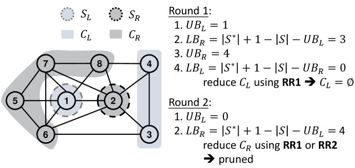
Example. To illustrate the proposed AltRB, consider an example in Figure 1 with $k$ =2, $|S^{*}|=5$ , $S=\{v_{1},v_{2}\}$ and $C=\{v_{3},v_{4},v_{5},v_{6},v_{7},v_{8}\}$ . First, we apply the greedy partition (Algorithm 3) and obtain $S_{L}=\{v_{1}\}$ , $S_{R}=\{v_{2}\}$ , $C_{L}=\{v_{3},v_{4}\}$ , and $C_{R}=\{v_{5},v_{6},v_{7},v_{8}\}$ . Then, in the first round of AltRB (Lines 4-7 in Algorithm 2), we conduct the four steps. (Step 1) Compute the upper bound of $C_{L}$ , i.e., $UB_{L}=1$ . (Step 2) Update the lower bound of $C_{R}$ (i.e., $LB_{R}=3$ ) and reduce $C_{R}$ via RR1 and RR2 (no vertices are removed). (Step 3) Compute the upper bound of $C_{R}$ , i.e., $UB_{R}=4$ . (Step 4) Update the lower bound of $C_{L}$ (i.e., $LB_{R}=0$ ) and reduce $C_{L}$ via RR1 and RR2 ( $C_{L}$ is reduced to an empty set). Next, in the second round with $C_{L}=\emptyset$ , we (1) compute $UB_{L}=0$ , and (2) update $LB_{R}=4$ and reduce $C_{R}$ . If we first apply RR1 to $C_{R}$ , $v_{5},v_{6},v_{7}$ and $v_{8}$ will be removed, and finally compute the upper bound as $UB^{\star}=|S|+|UB_{L}|+|UB_{R}|=2+0+0=2$ , resulting in pruning. If we first apply RR2, both $UB_{L}+UB_{R}+|S|=|S^{*}|+1$ and $UB_{R}=|C_{R}|$ are satisfied. We then find that $G[S\cup C_{R}]$ is not a $k$ -plex, which means that RR2 also leads to pruning. Actually, the size of maximum 2-plex is 5, indicating that the branch $(S,C)$ cannot find a larger 2-plex, and thus this branch can be pruned by AltRB. However, without AltRB, the existing method (Jiang et al., 2023) will compute an upper bound as $UB=UB_{L}+UB_{R}+|S|=1+4+2=7$ , which cannot prune the current branch.

Remarks. We remark that the existing reduction rules proposed in (Chang et al., 2022; Wang et al., 2023; Chang and Yao, 2024) are all based on $|S^{*}|$ and thus orthogonal to AltRB. We conduct some of these reduction rules to improve practical performance, including (1) additional reduction on subgraph $g$ (Lemma 3.2 in (Chang et al., 2022) and Reduction 2 in (Wang et al., 2023)) in Line 5 of Algorithm 1, and (2) reduction on $C$ before AltRB (RR4 in (Chang et al., 2022) and Algorithm 3 in (Chang and Yao, 2024)). Besides, AltRB is also orthogonal to the branching rules for selecting the branching vertex and forming the sub-branches.

5. Efficient Pre-processing techniques

In this section, we develop some efficient pre-processing techniques for further boosting the performance of BRB algorithms, namely, CF-CTCP for reducing the size of the input graph in Section 5.1 and KPHeuris for heuristically computing a large $k$ -plex in Section 5.2.

5.1. Faster Core-Truss Co-Pruning: CF-CTCP

Let $lb$ be the lower bound of the size of the largest $k$ -plex (which corresponds to the size of the largest $k$ -plex $G[S^{*}]$ seen so far). We also let $\Delta(u,v)$ be the set of common neighbors of $u$ and $v$ in $G$ , i.e., $\Delta(u,v)=N_{G}(u)\cap N_{G}(v)$ . The idea of refining the input graph $G$ is to remove from $G$ those vertices and edges that cannot appear in any $k$ -plex larger than $lb$ as many as we can. Existing methods (Zhou et al., 2021; Chang et al., 2022; Jiang et al., 2023) are all based on the following lemmas and differ in the implementations (the details of proof is omitted for the ease of presentation).

Lemma 5.1.

(Core Pruning (Gao et al., 2018)) For each vertex $u\in V(G)$ , $u$ cannot appear in a $k$ -plex of size $lb+1$ if $d_{G}(u)\leq lb-k$ .

Lemma 5.2.

(Truss Pruning (Zhou et al., 2021)) For each edge $(u,v)\in E(G)$ , $(u,v)$ cannot appear in a $k$ -plex of size $lb+1$ if $\delta_{G}(u,v)\leq lb-2k$ where $\delta_{G}(u,v)$ is the number of common neighbors of $u$ and $v$ , i.e., $\delta_{G}(u,v)=|\Delta(u,v)|$ .

Note that the time complexities of core pruning and truss pruning are $O(m)$ (Batagelj and Zaveršnik, 2003) and $O(m\times\delta(G))$ (Wang and Cheng, 2012), respectively. The above lemmas (namely, core pruning and truss pruning) indicates those unpromising vertices and edges can be removed from $G$ . In particular, with some vertices or edges being removed from $G$ , the remaining vertices $u$ and edges $(u,v)$ have $d_{G}(u)$ and $\delta_{G}(u,v)$ decreases, respectively; and then more vertices and edges can be removed. Therefore, the core pruning (resp. the truss pruning) can be conducted in an iterative way, i.e., iteratively removing unpromising vertices (resp. edges) and updating $d_{G}(\cdot)$ (resp. $\delta_{G}(\cdot,\cdot)$ ) for the remaining until no vertex or edge can be removed. We remark that the state-of-the-art method called the core-truss co-pruning (CTCP (Chang et al., 2022)) iteratively conducts the truss pruning and then the core pruning in multiple rounds until the graph remains unchanged. However, we observe that CTCP is still inefficient due to potential redundant computations. This is because (1) CTCP performs the truss pruning and the core pruning separately at each round (i.e., first remove a set of edges via the truss pruning and then remove one unpromising vertex via core pruning), (2) the truss pruning has the time complexity of $O(m\times\delta(G))$ lager than $O(m)$ for the core pruning, and (3) we note that during the truss pruning, some vertices can be removed via the more efficient core pruning while the truss pruning will iteratively check all their incident edges and then remove some of them (which is very costly).

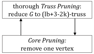
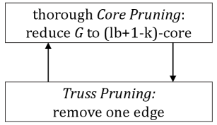
To improve the practical efficiency of CTCP, we propose a new algorithm called the core-pruning-first core-truss co-pruning (or CF-CTCP), which differs from CTCP in the way of conducting pruning at each round. Specifically, at each round, it first removes all unpromising vertices and then removes one unpromising edge (recall that CTCP first removes all unpromising edges and then one unpromising vertex). The benefit is that unpromising vertices can be removed immediately via efficient core pruning. Note that our CF-CTCP has the same output but requires less computation compared to CTCP. Given the integer $k$ and the lower bound $lb$ , both CF-CTCP and CTCP reduce the input graph $G$ to the maximal subgraph that is $(lb+1-k)$ -core and $(lb+3-2k)$ -truss. The difference between CF-CTCP and CTCP is illustrated in Figure 2.

The main idea of CF-CTCP is to conduct core pruning thoroughly as follows: 1) if we identify an edge that can be removed, we will immediately remove this edge, even if we have not yet finished computing $\Delta(\cdot,\cdot)$ (i.e., all triangles for each edge); 2) after removing an edge $(u,v)$ , we will check whether $u$ or $v$ can be reduced by core pruning. Note that after removing an edge $(u,v)$ , we postpone the action of updating $\Delta(u,\cdot)$ and $\Delta(v,\cdot)$ since it is time-consuming and there may lead to redundant computations. For example, if both vertices $u$ and $v$ will be removed by core pruning later, updating $\Delta(u,\cdot)$ and $\Delta(v,\cdot)$ is not necessary.

Our proposed CF-CTCP is shown in Algorithm 4. The input of CF-CTCP includes: 1) a set of vertices $Q_{v}$ , which stores the vertices that need to be removed; 2) two integers $\tau_{v}=lb-k$ and $\tau_{e}=lb-2k$ that serve as thresholds for the numbers of degrees and triangles for pruning, respectively; 3) a boolean value $lb\_changed$ which is $true$ if a larger $k$ -plex is found in kPEX and KPHeuris (Algorithm 1 and Algorithm 5). We note that both kPEX and KPHeuris (Algorithms 1 and 5) invoke CF-CTCP multiple times. For example, KPHeuris invokes CF-CTCP by calling CF-CTCP $(G,\emptyset,lb-k,lb-2k,true)$ when it finds a larger heuristic $k$ -plex of size $lb$ .

We then describe the details of CF-CTCP in steps. First, we design a procedure called RemoveEdge (Lines 21-24) to remove one unpromising edge in Line 21 and all current unpromising vertices in Line 22 via core and truss pruning. The set of removed edges to be considered (due to Lines 21 and 22) is pushed into $Q_{e}$ , which will be used to update $\Delta(\cdot,\cdot)$ later. Second, Lines 5-6 initialize the sets of common neighbours $\Delta(\cdot,\cdot)$ if CF-CTCP is invoked for the first time. Whenever we find an edge $(u,v)$ that can be reduced, we invoke the procedure RemoveEdge to remove $(u,v)$ immediately in Line 8. Third, we postpone the action of updating $\Delta(\cdot,\cdot)$ to Lines 9-20. Lines 11-20 consider the effect of each removed edge $(u,v)$ by traversing all the triangles that $(u,v)$ participates in. Specifically, Lines 11-15 traverse each edge $(u,w)\in E$ satisfying $v\in\Delta(u,w)$ , i.e., $u,v,w$ can form a triangle, then we update $\Delta(u,w)$ and check whether edge $(u,w)$ can be reduced. Lines 16-20 consider the edges connected to $v$ , which is similar to Lines 11-15. Note that in Lines 15 and 20, if we find an edge that can be reduced, we invoke the procedure RemoveEdge to remove the edge immediately.

Input: A graph

G=(V,E)

, the set of vertices to be removed

Q_{v}

, two integral thresholds

\tau_{v}

and

\tau_{e}

, a boolean value

lb\_changed

Output: The reduced graph which is the maximal subgraph in

G

that is both a

(\tau_{v}+1)

-core and a

(\tau_{e}+3)

-truss

1 Remove the vertices in

Q_{v}

from

G

and reduce

G

to the maximal

(\tau_{v}+1)

-core by the core pruning;

2 Initialize the set of removed edges to be considered

Q_{e}\leftarrow\{

edges removed at Line 1

\}

;

3 if $lb\_changed$ then

4 for each $(u,v)\in E$ do

5 if CF-CTCP is invoked for the first time then

\Delta(u,v)\leftarrow N_{G}(u)\cap N_{G}(v)

;

8 if $|\Delta(u,v)|\leq\tau_{e}$ then

Q_{e}\leftarrow Q_{e}\cup

RemoveEdge

(G,(u,v),\tau_{v})

;

13while $Q_{e}\neq\emptyset$ do

(u,v)\leftarrow

pop an edge from

Q_{e}

;

15 if $u\in V$ then

16 for each $w\in N_{G}(u)$ satisfying $v\in\Delta(u,w)$ do

17 Remove

v

from

\Delta(u,w)

;

18 if $|\Delta(u,w)|\leq\tau_{e}$ then

Q_{e}\leftarrow Q_{e}\cup

RemoveEdge

(G,(u,w),\tau_{v})

;

23 if $v\in V$ then

24 for each $w\in N_{G}(v)$ satisfying $u\in\Delta(v,w)$ do

25 Remove

u

from

\Delta(v,w)

;

26 if $|\Delta(v,w)|\leq\tau_{e}$ then

Q_{e}\leftarrow Q_{e}\cup

RemoveEdge

(G,(v,w),\tau_{v})

;

Procedure: RemoveEdge

(G,(u,v),\tau_{v})

Output: The set of removed edges to be considered

Q_{e}

33 Remove the unpromising edge

(u,v)

from

G

;

34 Reduce

G

to the maximal

(\tau_{v}+1)

-core by the core pruning;

35 Initialize the set of removed edges to be considered

Q_{e}\leftarrow\{

edges removed at Lines 21-22

\}

;

36 return

Q_{e}

;

Algorithm 4 CF-CTCP

(G=(V,E),Q_{v},\tau_{v},\tau_{e},lb\_changed)

Time complexity. We analyze the time complexity of CF-CTCP (Algorithm 4), including all invocations in kPEX, in the following.

Lemma 5.3.

The total time complexity of all invocations in kPEX (Algorithm 1 which includes invocations in the heuristic process KPHeuris in Algorithm 5)) to CF-CTCP (Algorithm 4) is $O(m\times\delta(G))$ .

The omitted proof, along with an implementation of CF-CTCP with $O(m)$ memory usage, is provided in the appendix.

Remarks. First, the time complexity of CTCP is $O(m\times\delta(G)+m\times k)$ = $O(m\delta(G))$ , requiring that $k$ is a small constant. However, $k$ is up to $n$ in theory and the time complexity of our CF-CTCP is always $O(m\delta(G))$ for all possible values of $k$ . Second, we do not consider the update of $\Delta(\cdot,\cdot)$ when removing a vertex because removing a vertex is equivalent to first removing all the edges connected to this vertex and then removing this isolated vertex. Therefore, we only consider the removed edges for updating $\Delta(\cdot,\cdot)$ . Third, the acceleration of CF-CTCP can be attributed to two main factors: 1) we do not need to compute the numbers of triangles for the edges that can be removed by core pruning; 2) for an edge $(u,v)$ to be removed such that both $u$ and $v$ are already removed by core pruning, we do not need to traverse related triangles to update $\Delta(\cdot,\cdot)$ . Note that if we cannot remove any vertex or edge, the time consumption of CF-CTCP will be the same as CTCP in theory, which is due to the fact that both of them need to compute $\Delta(\cdot,\cdot)$ in $O(m\times\delta(G))$ .

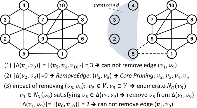
An example of CF-CTCP. Consider the example of CF-CTCP (Algorithm 4) in Figure 3, assuming $lb=4$ and $k=2$ . According to Lemma 5.1 and Lemma 5.2, we need to reduce $G$ to the maximal subgraph that is both a $3$ -core and a $3$ -truss, i.e., we will remove a vertex $u$ if $d_{G}(u)<3$ and an edge $(u,v)$ if $|\Delta(u,v)|<1$ . First, we enumerate each edge $(u,v)$ and compute the common neighbors of $u$ and $v$ (Lines 4-6). For those edges connected to $v_{1}$ , we cannot remove them since they have enough common neighbors, e.g., there are 3 common neighbors of $v_{1}$ and $v_{9}$ . However, when we consider edges connected to $v_{2}$ , we find that edge $(v_{2},v_{3})$ can be removed since $|\Delta(v_{2},v_{3})|=0$ . We then immediately remove edge $(v_{2},v_{3})$ and conduct core pruning, which removes vertices $v_{2},v_{3},v_{4}$ , and $v_{5}$ (Lines 21-24). After this process, we continue to compute common neighbors for the remaining edges, but none of these edges can be removed. Second, we begin to consider those removed edges in $Q_{e}$ . We focus on the edges $(v_{5},v_{9})$ and $(v_{1},v_{5})$ since the other removed edges cannot form a triangle with the remaining edges in $G$ . For the removal of the edge $(v_{5},v_{9})$ , according to Lines 11-20, we update $\Delta(v_{1},v_{9})$ , and the triangle $(v_{1},v_{5},v_{9})$ is destroyed. Then, for the edge $(v_{1},v_{5})$ , since the triangle $(v_{1},v_{5},v_{9})$ no longer exists after removing the edge $(v_{5},v_{9})$ , the edge $(v_{1},v_{5})$ cannot constitute any triangle with other vertices. Thus, the procedure of CF-CTCP terminates. Finally, we reduce $G$ to $G[\{v_{1},v_{6},v_{7},v_{8},v_{9},v_{10}\}]$ where $G[\{v_{1},v_{6},v_{8},v_{9},v_{10}\}]$ is a $2$ -plex of size $5$ .

5.2. Compute a large $k$ -plex: KPHeuris

We introduce a heuristic method KPHeuris for computing a large initial $k$ -plex. Note that such an initial $k$ -plex offers a lower bound $lb$ , which helps to narrow the search space; and the larger the lower bound is, the more search space can be refined. Therefore, KPHeuris is designed for obtaining a large $k$ -plex efficiently and effectively.

Input: A graph

G=(V,E)

and an integer

k>1

Output: The vertex set

S

of a heuristic initial

k

-plex

G[S]

S\leftarrow

Degen

(G,k)

lb\leftarrow|S|

;

3 Apply CF-CTCP for refining

G

based on

lb

;

4 for each $v_{i}\in V(G)$ do

g\leftarrow

G[\{v_{i},v_{i+1},...,v_{n}\}\cap N^{\leq 2}(v_{i})]

;

S^{\prime}\leftarrow

Degen

(g,k)

;

6 if $|S^{\prime}|>|S|$ then

S\leftarrow S^{\prime}

lb\leftarrow|S|

;

8 Apply CF-CTCP for refining

G

based on

lb

;

11return

S

;

Procedure: Degen

(G,k)

Output: The vertex set

S

of a heuristic maximal

k

-plex in

G

v_{1},v_{2},...,v_{n}\leftarrow

the degeneracy order of vertices in

V(G)

;

S\leftarrow\emptyset

;

15 for $i=n$ to $1$ do

16 if $G[S\cup\{v_{i}\}]$ is a $k$ -plex then

S\leftarrow S\cup\{v_{i}\}

;

18return

S

;

Algorithm 5 KPHeuris

(G,k)

We summarize KPHeuris in Algorithm 5, which relies on a sub-procedure (called Degen) for computing a large $k$ -plex. Specifically, Degen iteratively includes to an empty set $S$ a vertex in a graph $G$ based on the degeneracy ordering while retaining the $k$ -plex property of $G[S]$ until we cannot continue (Lines 9-12). To compute a larger $k$ -plexes, KPHeuris further generate $n$ subgraphs from $G$ , each of which corresponds to a vertex in $G$ (Lines 3-4); it then invokes Degen on each of them to obtain a $k$ -plex (Line 4); it finally returns the largest one among $n+1$ found $k$ -plexes. Note that the subgraph related to $v_{i}$ is the subgraph induced by $\{v_{i},v_{i+1},...,v_{n}\}\cap N^{\leq 2}(v_{i})$ where $N^{\leq 2}(u)$ denotes $u$ ’s neighbors and $u$ ’s neighbors’ neighbors, and the rationale is that it can make the subgraph smaller and denser, which tends to find a larger $k$ -plex easier. The time complexity of Degen is $O(m)$ , and we will invoke it at most $n+1$ times, thus the total time complexity of computing heuristic solutions in Algorithm 5 is $O(nm)$ . We remark that the total time complexity of all invocations of CF-CTCP is $O(m\delta(G))$ because we invoke CF-CTCP in KPHeuris only when we find a larger $k$ -plex, i.e., $lb\_changed=true$ , as shown in Lemma 5.3. Thus, the time complexity of KPHeuris is $O(m\delta(G)+nm)=O(nm)$ .

Compared with existing heuristic methods. There are two state-of-the-art heuristic methods: kPlex-Degen ((Chang et al., 2022)) and EGo-Degen ((Chang and Yao, 2024)). kPlex-Degen computes a large $k$ -plex by iteratively removing a vertex from the input graph $G$ based on a certain ordering until the remaining graph becomes a $k$ -plex. KPHeuris differs from kPlex-Degen in two aspects. First, Degen computes a large $k$ -plex by iteratively including a vertex, which is more efficient since the size of the largest $k$ -plex is usually much smaller than the size of the input graph (especially for real-world graphs) and can always return a maximal $k$ -plex, while kPlex-Degen cannot. Second, KPHeuris further explores $n$ subgraphs instead of the input graph $G$ , which tends to obtain a larger $k$ -plex as empirically verified in our experiments. EGo-Degen extracts a subgraph $g_{v}$ for each vertex $v$ and invokes kPlex-Degen to compute a $k$ -plex in $g_{v}$ . Then, EGo-Degen selects the largest $k$ -plex among those computed on $n$ subgraphs as the initial heuristic $k$ -plex. KPHeuris differs from EGo-Degen in three aspects. First, the method of subgraph extraction is different. For a vertex $v\in V(G)$ , EGo-Degen extracts $g_{v}=G[\{v_{i},v_{i+1},...,v_{n}\}\cap N_{G}(v_{i})]$ , while our KPHeuris generates a subgraph $g_{v}^{\prime}=G[\{v_{i},v_{i+1},...,v_{n}\}\cap N^{\leq 2}(v_{i})]$ . It is easy to verify that $g_{v}\subseteq g_{v}^{\prime}$ due to $N_{G}(v_{i})\subseteq N^{\leq 2}(v_{i})$ . Additionally, a larger subgraph tends to contain a larger $k$ -plex, as verified in Table 6. Second, EGo-Degen computes $k$ -plexes by invoking kPlex-Degen, which implies that it may find a non-maximal $k$ -plex as mentioned above. Third, once a larger $k$ -plex is found, KPHeuris updates $lb$ and removes unpromising vertices/edges immediately, while EGo-Degen does not reduce the graph until $n$ heuristic $k$ -plexes are computed.

6. Experimental Studies

We test the efficiency and effectiveness of our algorithm kPEX by comparing with the state-of-the-art BRB algorithms:

•

kPlexS ¹¹1https://github.com/LijunChang/Maximum-kPlex: the existing algorithm proposed in (Chang et al., 2022).
•

KPLEX ²²2https://github.com/joey001/kplex_degen_gap: the existing algorithm proposed in (Wang et al., 2023).
•

DiseMKP ³³3https://github.com/huajiang-ynu/ijcai23-kpx: the existing algorithm proposed in (Jiang et al., 2023).
•

kPlexT ⁴⁴4https://github.com/LijunChang/Maximum-kPlex-v2: the existing algorithm proposed in (Chang and Yao, 2024).

Setup. All algorithms are written in C++ and compiled with -O3 optimization by g++ 9.4.0. Moreover, all algorithms are initialized with a lower bound of $2k-2$ to focus on finding $k$ -plexes with at least $2k-1$ vertices. All experiments are conducted in the single-thread mode on a machine with an Intel(R) Xeon(R) Platinum 8358P CPU@2.60GHz and 256GB main memory. The CPU frequency is fixed at 3.3GHz. We set the time limit as 3600 seconds and use OOT (Out Of Time limit) to indicate the time exceeds the limit. We consider six different values of $k$ , i.e., $2,3,5,10,15$ , and $20$ . We focus on the case of $k=5$ , and defer the experiments for other values of $k$ to the appendix. We also note that the major findings for $k=5$ hold for other values of $k$ .

Datasets. We consider the following two collections of graphs.

•

Network Repository (Net, tory). The dataset contains 584 graphs with up to $5.87\times 10^{7}$ vertices, including biological networks (36), dynamic networks (85), labeled networks (104), road networks (15), interaction (29), scientific computing (11), social networks (75), facebook (114), web (31), and DIMACS-10 graphs (84). Most of them are real-world graphs.
•

2nd-DIMACS (DIMACS-2) Graphs (DIM, MACS). The dataset contains 80 synthetic dense graphs with up to 4000 vertices and the densities ranging from 0.03 to 0.99. Most graphs in the dataset are synthetic graphs, which are often hard to be solved (Jiang et al., 2021; Wang et al., 2023; Jiang et al., 2023).

For better comparisons, we select 30 representative graphs from the above 664 graphs and report the statistics in Table 1, where the graph density is $\frac{2m}{n(n-1)}$ and the maximum degree is $d_{max}$ . The criteria of selecting these representative graphs are as follows. First, following (Wang et al., 2023), we do not select extremely easy or hard graphs, i.e., those graphs that can be solved within 5 seconds by all five solvers or cannot be solved within 3600 seconds by any solver when $k=5$ . Second, the representative graphs cover a wide range of sizes. Among the selected graphs, 10 small dense graphs (G1-G10) are synthetic graphs from DIMACS-2 Graphs, 10 medium graphs (G11-G20) with at most $10^{6}$ vertices, and 10 large sparse graphs (G21-G30) with at least $10^{6}$ vertices are real-world graphs from Network Repository. Third, most of the representative graphs have also been selected in previous studies (Jiang et al., 2021; Wang et al., 2023; Xiao et al., 2017).

Table 1. Statistics of 30 representative graphs

ID	Graph	$n$	$m$	density	$d_{max}$	$\delta(G)$
G1	johnson8-4-4	70	1855	$7.68\cdot 10^{-1}$	53	53
G2	C125-9	125	6963	$8.98\cdot 10^{-1}$	119	102
G3	keller4	171	9435	$6.49\cdot 10^{-1}$	124	102
G4	brock200-2	200	9876	$4.96\cdot 10^{-1}$	114	84
G5	san200-0-9-1	200	17910	$9.00\cdot 10^{-1}$	191	162
G6	san200-0-9-2	200	17910	$9.00\cdot 10^{-1}$	188	169
G7	san200-0-9-3	200	17910	$9.00\cdot 10^{-1}$	187	169
G8	p-hat300-1	300	10933	$2.44\cdot 10^{-1}$	132	49
G9	p-hat300-2	300	21928	$4.89\cdot 10^{-1}$	229	98
G10	p-hat500-1	500	31569	$2.53\cdot 10^{-1}$	204	86
G11	soc-BlogCatalog-ASU	10312	333983	$6.28\cdot 10^{-3}$	3992	114
G12	socfb-UIllinois	30795	1264421	$2.67\cdot 10^{-3}$	4632	85
G13	soc-themarker	69413	1644843	$6.83\cdot 10^{-4}$	8930	164
G14	soc-BlogCatalog	88784	2093195	$5.31\cdot 10^{-4}$	9444	221
G15	soc-buzznet	101163	2763066	$5.40\cdot 10^{-4}$	64289	153
G16	soc-LiveMocha	104103	2193083	$4.05\cdot 10^{-4}$	2980	92
G17	soc-wiki-conflict	116836	2027871	$2.97\cdot 10^{-4}$	20153	145
G18	soc-google-plus	211187	1141650	$5.12\cdot 10^{-5}$	1790	135
G19	soc-FourSquare	639014	3214986	$1.57\cdot 10^{-5}$	106218	63
G20	rec-epinions-user-ratings	755760	13667951	$4.79\cdot 10^{-5}$	162179	151
G21	soc-wiki-Talk-dir	1298165	2288646	$2.72\cdot 10^{-6}$	100025	119
G22	soc-pokec	1632803	22301964	$1.67\cdot 10^{-5}$	14854	47
G23	tech-ip	2250498	21643497	$8.55\cdot 10^{-6}$	1833161	253
G24	ia-wiki-Talk-dir	2394385	4659565	$1.63\cdot 10^{-6}$	100029	131
G25	sx-stackoverflow	2584164	28183518	$8.44\cdot 10^{-6}$	44065	198
G26	web-wikipedia_link_it	2790239	86754664	$2.23\cdot 10^{-5}$	825147	894
G27	socfb-A-anon	3097165	23667394	$4.93\cdot 10^{-6}$	4915	74
G28	soc-livejournal-user-groups	7489073	112305407	$4.00\cdot 10^{-6}$	1053720	116
G29	soc-bitcoin	24575382	86063840	$2.85\cdot 10^{-7}$	1083703	325
G30	soc-sinaweibo	58655849	261321033	$1.52\cdot 10^{-7}$	278489	193

6.1. Comparing with State-of-the-art Algorithms

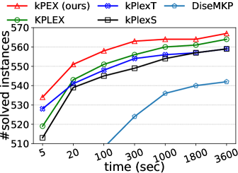
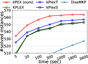
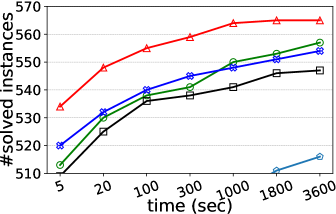
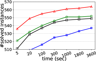
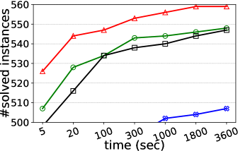
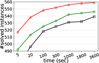
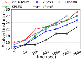
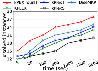
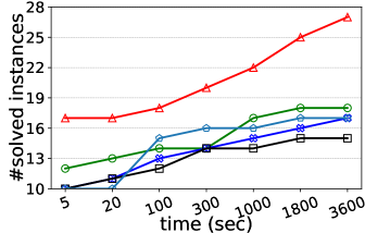
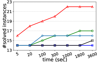
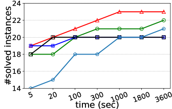
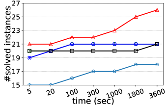
Number of solved instances on two collections of graphs. We compare kPEX with four baselines by reporting the numbers of solved instances. The results for Network Repository are shown in Table 2 and Figure 4. We observe that kPEX outperforms all baselines for all tested values of $k$ . For example, kPEX solves 12 instances more than the best baseline KPLEX for $k=10$ within 3600 seconds. In addition, our kPEX is more stable than baselines when varying $k$ . In contrast, there is an obvious drop in solved instances for kPlexT and DiseMKP as $k$ increases from 2 to 20. This demonstrates the superiority of kPEX, which employs the AltRB strategy (with novel reduction and bounding techniques) and efficient pre-processing methods. The results on the collection of DIMACS-2 Graphs are shown in Table 3 and Figure 5. kPEX outperforms all baselines by solving the most instances with 3600 seconds for all tested $k$ values, e.g., kPEX solves 9 instances more than the second best solver KPLEX for $k=5$ . Besides, we note that kPEX is comparable with DiseMKP when $k=2$ . This is because the proposed reduction rules and upper bounding method are less effective for small values of $k$ .

Table 2. Number of solved instances on Network Repository within 3600 seconds

$k$	kPEX (ours)	KPLEX	kPlexT	kPlexS	DiseMKP
2	567	564	559	559	542
3	564	553	557	553	527
5	565	557	554	547	516
10	564	552	537	549	495
15	559	548	507	547	452
20	559	546	471	539	439

Table 3. Number of solved instances on DIMACS-2 within 3600 seconds

$k$	kPEX (ours)	KPLEX	kPlexT	kPlexS	DiseMKP
2	29	27	25	22	27
3	28	23	24	20	25
5	27	18	17	15	17
10	22	17	14	15	16
15	23	22	20	20	21
20	26	21	21	21	18

Running times on representative graphs. We report the running times of all algorithms on 30 representative graphs with $k=5$ in Table 4. We observe that kPEX outperforms all baselines by achieving significant speedups on the majority graphs. For example, kPEX runs at least 5 times faster than KPLEX on 25 out of 30 graphs and at least 5 times faster than kPlexT on 21 out of 30 graphs. Moreover, there are 7 out of 30 graphs where kPEX runs at least 100 times faster than all baselines. Note that kPEX may exhibit slower performance compared to baselines on rare occasions. For instance, the baseline kPlexT runs faster than our kPEX on G23 with $k=5$ . The possible reasons include: 1) All algorithms rely on some heuristic procedures, e.g., the heuristic method for finding a large initial $k$ -plex. The performance of these heuristic methods varies across different graphs and settings; 2) Compared with baselines, kPEX incorporates newly proposed reduction techniques, which may introduce additional time costs.

Table 4. Running time in seconds of kPEX and state-of-the-arts on 30 graphs with

k=5

ID	kPEX (ours)	KPLEX	kPlexT	kPlexS	DiseMKP
G1	3.88	1154.76	120.63	187.88	55.56
G2	1360.94	OOT	OOT	OOT	OOT
G3	1527.41	OOT	OOT	OOT	OOT
G4	306.14	OOT	3160.85	OOT	OOT
G5	0.10	0.29	34.09	1356.45	0.16
G6	24.63	OOT	OOT	OOT	OOT
G7	433.86	OOT	OOT	OOT	OOT
G8	2.22	567.84	20.91	OOT	27.92
G9	2.82	411.26	OOT	OOT	OOT
G10	191.31	OOT	1339.31	OOT	1133.52
G11	3.97	1766.68	2318.35	OOT	OOT
G12	0.39	1.30	0.53	1.36	440.90
G13	55.29	OOT	OOT	OOT	OOT
G14	927.11	OOT	OOT	OOT	OOT
G15	21.17	OOT	OOT	OOT	OOT
G16	1.68	58.82	27.28	1655.40	900.80
G17	1.68	3022.10	123.86	OOT	OOT
G18	0.72	2804.46	1818.90	1099.39	OOT
G19	0.64	3.59	2.15	2.06	1695.05
G20	4.39	795.20	204.00	72.03	1347.27
G21	2.82	961.06	1515.40	OOT	OOT
G22	2.42	13.58	3.72	11.77	18.25
G23	13.16	136.61	4.80	11.39	OOT
G24	5.61	2979.37	3055.73	OOT	OOT
G25	3.80	92.05	203.26	OOT	OOT
G26	4.84	700.66	7.25	39.25	8.41
G27	2.60	14.52	3.50	15.39	51.94
G28	139.52	OOT	OOT	1703.49	OOT
G29	6.08	312.93	OOT	OOT	OOT
G30	593.26	OOT	OOT	OOT	OOT

6.2. Effectiveness of Proposed Techniques

We compare the running time of kPEX with its variants:

•

kPEX-SeqRB: kPEX replaces AltRB with SeqRB(Section 4).
•

kPEX-CTCP: kPEX replaces CF-CTCP with CTCP ((Chang et al., 2022)).
•

kPEX-EGo: kPEX replaces KPHeuris with the existing heuristic method EGo-Degen in (Chang and Yao, 2024).
•

kPEX-Degen: kPEX replaces KPHeuris with the existing heuristic method kPlex-Degen in (Chang et al., 2022).

In other words, kPEX-SeqRB is the version without AltRB; kPEX-CTCP is the version without CF-CTCP; kPEX-EGo and kPEX-Degen are the versions without KPHeuris.

Table 5. Running time in seconds of kPEX and its variants on 30 graphs with

k=5

ID	kPEX	kPEX-SeqRB	kPEX-CTCP	kPEX-EGo	kPEX-Degen
G1	3.88	18.66	3.89	3.91	3.92
G2	1360.94	OOT	1364.70	1371.95	1365.94
G3	1527.41	OOT	1525.00	1539.98	1538.84
G4	306.14	3220.90	305.95	307.76	307.69
G5	0.10	0.11	0.10	0.10	0.09
G6	24.63	557.07	24.63	33.37	57.68
G7	433.86	OOT	434.65	528.89	674.42
G8	2.22	18.54	2.22	2.19	2.20
G9	2.82	20.47	2.81	4.21	4.18
G10	191.31	3472.65	191.72	202.50	202.49
G11	3.97	23.51	4.63	4.19	3.87
G12	0.39	0.39	2.24	0.88	0.71
G13	55.29	555.36	59.38	97.39	103.23
G14	927.11	OOT	936.52	1113.52	1197.87
G15	21.17	128.27	35.76	29.85	24.84
G16	1.68	2.19	5.84	2.35	2.18
G17	1.68	8.49	8.27	3.88	1.90
G18	0.72	6.76	1.34	0.90	0.66
G19	0.64	0.66	17.41	8.36	93.70
G20	4.39	4.46	222.02	150.66	260.41
G21	2.82	8.03	3.55	3.68	3.32
G22	2.42	2.26	16.82	8.28	2.40
G23	13.16	12.62	1618.38	461.19	117.33
G24	5.61	15.80	6.97	9.83	9.03
G25	3.80	3.56	66.56	22.87	3.69
G26	4.84	4.77	4.64	5.61	4.54
G27	2.60	2.48	24.83	11.07	2.63
G28	139.52	139.96	OOT	OOT	OOT
G29	6.08	17.57	5.99	11.18	10.85
G30	593.26	OOT	1628.00	2094.29	2020.66

Effectiveness of AltRB. We compare kPEX with kPEX-SeqRB and report the running times in Table 5. We observe that kPEX performs better than kPEX-SeqRB by achieving at least a 5 $\times$ speedup on 12 out of 30 graphs and running up to 20 $\times$ faster on G6. This indicates the effectiveness of AltRB in narrowing down the search space. Besides, AltRB contributes more speedups on synthetic graphs G1-G10 since the running time is dominated by the branch-reduction-and-bound stage on these graphs.

Table 6. Pre-processing time in seconds on 20 graphs with

k

=5 (

lb

denotes the size of the computed heuristic

k

-plex)

ID	kPEX		kPlexT		kPlexS		DiseMKP
ID	time	$lb$	time	$lb$	time	$lb$	time	$lb$
G11	0.43	51	0.41	50	0.30	50	0.53	49
G12	0.39	73	0.58	69	1.30	34	1.71	34
G13	4.35	39	1.69	37	2.44	36	3.85	35
G14	9.24	70	5.01	67	3.08	64	6.05	66
G15	3.06	49	2.06	48	4.08	48	10.59	47
G16	1.29	27	0.82	26	1.84	14	3.85	14
G17	0.68	39	0.62	37	1.69	37	5.53	37
G18	0.14	87	0.34	87	0.27	87	0.51	87
G19	0.63	44	2.08	42	0.93	37	9.60	37
G20	3.48	21	33.60	19	32.56	10	118.24	10
G21	0.64	44	0.37	43	0.43	43	0.66	42
G22	2.42	34	4.51	32	15.46	26	15.55	27
G23	13.16	11	5.91	11	13.05	10	1708.75	10
G24	1.28	44	0.67	41	0.94	41	1.40	41
G25	3.14	77	7.90	76	34.82	76	45.58	77
G26	2.90	881	3.57	881	3.94	881	3.90	880
G27	2.60	37	4.79	35	18.02	32	21.06	33
G28	102.57	17	719.41	15	1210.59	12	OOT	-
G29	2.74	296	3.17	292	3.31	292	8.52	292
G30	102.73	65	134.74	62	252.29	17	1217.99	16

Effectiveness of CF-CTCP. We compare kPEX with kPEX-CTCP, and the running times are reported in Table 5. First, kPEX and kPEX-CTCP have similar performance on G1-G10 because the pre-processing techniques take little time (e.g., less than 1 second) on these synthetic graphs. Second, kPEX runs at least 5 times faster than kPEX-CTCP on 8 out of 20 real-world graphs. Moreover, CF-CTCP provides at least 50 $\times$ speedup on G20 and G23. These results show the effectiveness of CF-CTCP on large sparse graphs.

Effectiveness of KPHeuris. We compare kPEX with its variants kPEX-EGo and kPEX-Degen (note that CF-CTCP is not replaced). The running times are shown in Table 5. We have the following observations. First, the running time of kPEX is less than that of both variants on the majority of graphs (i.e., on 23 out of 30 graphs). Then, kPEX runs at least 5 times faster than kPEX-EGo on 5 out of 30 graphs and faster than kPEX-Degen on 4 out of 30 graphs. In addition, kPEX runs at least 25 times faster than both kPEX-EGo and kPEX-Degen on G20 and G28. This shows that making more effort to finding a larger initial $k$ -plex benefits kPEX by narrowing down the search space. Second, although kPEX may be slightly slower than the two variants, the extra time consumption is small and can be ignored compared to the total running time. For example, kPEX is 0.1 seconds slower than kPEX-Degen on G11 due to the extra computation, while the total running time of kPEX is 3.97 seconds, which means that the extra time consumption is negligible. Third, the performance of kPEX-EGo and kPEX-Degen is better than kPEX-SeqRB on G1-G10. This means that the variant of kPEX without AltRB is slower than the variant without KPHeuris. This indicates that AltRB provides a greater performance boost than heuristic techniques on those graphs where branch-reduction-and-bound stage dominates the running time.

Effectiveness of KPHeuris and CF-CTCP. We also compare the total pre-processing time and the size of the $k$ -plex (i.e., $lb$ ) obtained by different heuristic methods in kPEX, kPlexT, kPlexS, and DiseMKP (note that KPLEX uses the same pre-processing method as kPlexS). The results are reported in Table 6. Note that we exclude the results on synthetic graphs G1-G10 since they have only hundreds of vertices and can be handled within 1 second by all methods. We have the following observations. First, kPEX consistently obtains the largest $lb$ (or matches the largest obtained by others) while the pre-processing time remains comparable to other algorithms. Second, KPHeuris outperforms the other pre-processing algorithms by obtaining a lager $k$ -plex while costing much less time on G20 and G28. This also verifies the effectiveness of CF-CTCP and KPHeuris.

7. Related work

Maximum $k$ -plex search. The maximum $k$ -plex search problem has garnered significant attention in social network analysis (McClosky and Hicks, 2012; Moser et al., 2012) since the concept of $k$ -plex was first proposed in (Seidman and Foster, 1978). Balasundaram et al. (Balasundaram et al., 2011) showed the NP-hardness of the problem with any fixed $k$ . Consequently, the major algorithmic design paradigm for exact solution is based on the branch-reduction-and-bound (BRB) framework (Xiao et al., 2017; Wang et al., 2023; Gao et al., 2018; Zhou et al., 2021; Jiang et al., 2021; Chang et al., 2022; Jiang et al., 2023; Chang and Yao, 2024). In particular, Xiao et al. (Xiao et al., 2017) proposed a branching strategy, which improves theoretical time complexity from the trivial bound of $O^{*}(2^{n})$ to $O^{*}(c^{n})$ where $c<2$ and $O^{*}$ ignores polynomial factors. Later, Wang et al. (Wang et al., 2023) designed KPLEX which is parameterized by the degeneracy gap (bounded empirically by $O(\log n)$ ). Very recently, Chang and Yao (Chang and Yao, 2024) proposed kPlexT, which improves the worst-case time complexity with newly proposed branching and reduction techniques. Additionally, several reduction and bounding techniques have been designed in the BRB framework to boost the practical performance. Gao et al. (Gao et al., 2018) developed reduction methods and a dynamic vertex selection strategy. Later, Zhou et al. (Zhou et al., 2021) proposed a stronger reduction method and designed a coloring-based bounding method. Jiang et al. (Jiang et al., 2021) designed a partition-based bounding method, and later in (Jiang et al., 2023), their algorithm DiseMKP is equipped with a better upper bound. Chang et al. (Chang et al., 2022) designed an efficient algorithm kPlexS with a novel reduction method CTCP and a heuristic method. We note that the algorithms designed by Xiao et al. (Xiao et al., 2017) and Chang and Yao (Chang and Yao, 2024) also work for the case when there is no requirement for the found $k$ -plex to be of size at least $2k-1$ . We remark that existing works mainly focus on the BRB framework that conducts the reduction and the bounding sequentially, and our solution kPEX firstly adopts a new BRB framework that alternatively and iteratively conducts the reduction and the bounding.

Maximal $k$ -plex enumeration. Another related problem is maximal $k$ -plex enumeration, which aims to list all all maximal $k$ -plexes in the input graph; Here, a $k$ -plex is maximal if it cannot be contained in other $k$ -plexes. Many efficient algorithms are proposed for enumerating maximal $k$ -plexes, including Bron-Kerbosch-based algorithms (Wu and Pei, 2007; Wang et al., 2017; Conte et al., 2018, 2017; Dai et al., 2022b; Wang et al., 2022) and reverse-search-based algorithms (Berlowitz et al., 2015). We remark that existing algorithms for enumerating maximal $k$ -plexes can be utilized to solve the studied problem by listing all maximal $k$ -plexes and then returning the largest one among them (note that the maximum $k$ -plex is the maximal $k$ -plex with largest number of vertices). However, the resulting solutions are not efficient due to the limited pruning and bounding techniques, as verified in (Chang and Yao, 2024).

Other cohesive subgraph models. $k$ -plexes reduce to cliques when $k=1$ . There have been lines of work focusing on the maximum clique search and maximal clique enumeration problems (Carraghan and Pardalos, 1990; Pardalos and Xue, 1994; Tomita, 2017; Chang, 2019; Conte et al., 2016; Eppstein et al., 2013; Naudé, 2016; Tomita et al., 2006). Further, the concept of $k$ -plex is also explored in other kinds of graphs, e.g., bipartite graphs (Yu et al., 2022; Yu and Long, 2023b; Luo et al., 2022; Chen et al., 2021a; Dai et al., 2023b), directed graphs (Gao et al., 2024), temporal graphs (Bentert et al., 2019), uncertain graphs (Dai et al., 2022a), and so on. Besides $k$ -plex, various cohesive subgraph models have been studied, including $k$ -core (Batagelj and Zaveršnik, 2003; Cheng et al., 2011), $k$ -truss (Cohen, 2008; Huang et al., 2014; Wang and Cheng, 2012), $\gamma$ -quasi-clique (Pei et al., 2005; Zeng et al., 2006; Khalil et al., 2022; Yu and Long, 2023a), $k$ -defective clique (Chang, 2023; Dai et al., 2023a; Gao et al., 2022; Chen et al., 2021b), densest subgraph (Ma et al., 2021; Xu et al., 2024), and so on. For an overview on cohesive subgraph search, we refer to excellent books and surveys (Lee et al., 2010; Chang and Qin, 2018; Huang et al., 2019; Fang et al., 2020, 2021).

8. Conclusion

In this paper, we studied the maximum $k$ -plex search problem. We proposed a new branch-reduction-and-bound method, called kPEX, which includes a new alternated reduction-and-bound process AltRB. In addition, we also designed efficient pre-processing techniques for boosting the performance, which includes KPHeuris for computing a large heuristic $k$ -plex and CF-CTCP for efficiently removing unpromising vertices/edges. Extensive experiments on 664 graphs verified kPEX’s superiority over state-of-the-art algorithms. In the future, we will explore the possibility of adapting kPEX to mining other cohesive subgraphs.

References

(1)
DIM (MACS) 2nd-DIMACS. http://archive.dimacs.rutgers.edu/pub/challenge/graph/.
Net (tory) Network Repository. https://networkrepository.com/index.php.
Balasundaram et al. (2011) Balabhaskar Balasundaram, Sergiy Butenko, and Illya V. Hicks. 2011. Clique Relaxations in Social Network Analysis: The Maximum $k$ -Plex Problem. Operations Research 59, 1 (2011), 133–142.
Batagelj and Zaveršnik (2003) Vladimir Batagelj and Matjaž Zaveršnik. 2003. An ${O}(m)$ Algorithm for Cores Decomposition of Networks. CoRR cs.DS/0310049 (2003).
Bentert et al. (2019) Matthias Bentert, Anne-Sophie Himmel, Hendrik Molter, Marco Morik, Rolf Niedermeier, and René Saitenmacher. 2019. Listing All Maximal $k$ -Plexes in Temporal Graphs. ACM J. Exp. Algorithmics 24, Article 1.13 (Sep 2019).
Berlowitz et al. (2015) Devora Berlowitz, Sara Cohen, and Benny Kimelfeld. 2015. Efficient Enumeration of Maximal $k$ -Plexes. In Proc. ACM SIGMOD Int. Conf. Manage. Data (SIGMOD). 431–444.
Carraghan and Pardalos (1990) Randy Carraghan and Panos M. Pardalos. 1990. An Exact Algorithm for the Maximum Clique Problem. Operations Research Letter 9, 6 (1990), 375–382.
Chang (2019) Lijun Chang. 2019. Efficient Maximum Clique Computation over Large Sparse Graphs. In Proc. ACM SIGKDD Int. Conf. Knowl. Discov. Data Mining (SIGKDD). 529–538.
Chang (2023) Lijun Chang. 2023. Efficient Maximum $k$ -Defective Clique Computation with Improved Time Complexity. Proceedings of the ACM on Management of Data (SIGMOD) 1, 3 (2023), 1–26.
Chang and Qin (2018) Lijun Chang and Lu Qin. 2018. Cohesive Subgraph Computation over Large Sparse Graphs. Springer.
Chang et al. (2022) Lijun Chang, Mouyi Xu, and Darren Strash. 2022. Efficient Maximum $k$ -Plex Computation over Large Sparse Graphs. Proceedings of the VLDB Endowment 16, 2 (2022), 127–139.
Chang and Yao (2024) Lijun Chang and Kai Yao. 2024. Maximum $k$ -Plex Computation: Theory and Practice. Proceedings of the ACM on Management of Data (SIGMOD) 2, 1 (2024), 1–26.
Chen et al. (2021a) Lu Chen, Chengfei Liu, Rui Zhou, Jiajie Xu, and Jianxin Li. 2021a. Efficient Exact Algorithms for Maximum Balanced Biclique Search in Bipartite Graphs. In Proc. ACM SIGMOD Int. Conf. Manage. Data (SIGMOD). 248–260.
Chen et al. (2021b) Xiaoyu Chen, Yi Zhou, Jin-Kao Hao, and Mingyu Xiao. 2021b. Computing Maximum $k$ -Defective Cliques in Massive Graphs. Computers & Operations Research 127 (2021), 105131.
Cheng et al. (2011) James Cheng, Yiping Ke, Shumo Chu, and M Tamer Özsu. 2011. Efficient Core Decomposition in Massive Networks. In Proceedings of the IEEE International Conference Data Engineering (ICDE). 51–62.
Cohen (2008) Jonathan Cohen. 2008. Trusses: Cohesive Subgraphs for Social Network Analysis. National Security Agency Technical Report 16, 3.1 (2008).
Conte et al. (2018) Alessio Conte, Tiziano De Matteis, Daniele De Sensi, Roberto Grossi, Andrea Marino, and Luca Versari. 2018. D2K: Scalable Community Detection in Massive Networks via Small-Diameter $k$ -Plexes. In Proc. ACM SIGKDD Int. Conf. Knowl. Discov. Data Mining (SIGKDD). 1272–1281.
Conte et al. (2016) Alessio Conte, Roberto De Virgilio, Antonio Maccioni, Maurizio Patrignani, Riccardo Torlone, et al. 2016. Finding All Maximal Cliques in Very Large Social Networks. In Proceedings of the International Conference on Extending Database Technology (EDBT). 173–184.
Conte et al. (2017) Alessio Conte, Donatella Firmani, Caterina Mordente, Maurizio Patrignani, and Riccardo Torlone. 2017. Fast Enumeration of Large $k$ -Plexes. In Proc. ACM SIGKDD Int. Conf. Knowl. Discov. Data Mining (SIGKDD). 115–124.
Dai et al. (2022a) Qiangqiang Dai, Rong-Hua Li, Meihao Liao, Hongzhi Chen, and Guoren Wang. 2022a. Fast Maximal Clique Enumeration on Uncertain Graphs: A Pivot-based Approach. In Proc. ACM SIGMOD Int. Conf. Manage. Data (SIGMOD). 2034–2047.
Dai et al. (2023a) Qiangqiang Dai, Rong-Hua Li, Meihao Liao, and Guoren Wang. 2023a. Maximal Defective Clique Enumeration. Proc. ACM SIGMOD Int. Conf. Manage. Data (SIGMOD) 1, 1 (2023), 1–26.
Dai et al. (2022b) Qiangqiang Dai, Rong-Hua Li, Hongchao Qin, Meihao Liao, and Guoren Wang. 2022b. Scaling Up Maximal $k$ -Plex Enumeration. In Proceedings of the ACM International Conference on Information and Knowledge Management (CIKM). 345–354.
Dai et al. (2023b) Qiangqiang Dai, Rong-Hua Li, Xiaowei Ye, Meihao Liao, Weipeng Zhang, and Guoren Wang. 2023b. Hereditary Cohesive Subgraphs Enumeration on Bipartite Graphs: The Power of Pivot-based Approaches. Proc. ACM SIGMOD Int. Conf. Manage. Data (SIGMOD) 1, 2 (2023), 1–26.
Eppstein et al. (2013) David Eppstein, Maarten Löffler, and Darren Strash. 2013. Listing All Maximal Cliques in Large Sparse Real-World Graphs. ACM J. Exp. Algorithmics 18, Article 3.1 (Nov 2013).
Fang et al. (2020) Yixiang Fang, Xin Huang, Lu Qin, Ying Zhang, Wenjie Zhang, Reynold Cheng, and Xuemin Lin. 2020. A Survey of Community Search over Big Graphs. The VLDB Journal 29 (2020), 353–392.
Fang et al. (2021) Yixiang Fang, Kai Wang, Xuemin Lin, and Wenjie Zhang. 2021. Cohesive Subgraph Search over Big Heterogeneous Information Networks: Applications, Challenges, and Solutions. In Proc. ACM SIGMOD Int. Conf. Manage. Data (SIGMOD). 2829–2838.
Gao et al. (2018) Jian Gao, Jiejiang Chen, Minghao Yin, Rong Chen, and Yiyuan Wang. 2018. An Exact Algorithm for Maximum $k$ -Plexes in Massive Graphs. In Proceedings of the International Joint Conference on Artificial Intelligence (IJCAI). 1449–1455.
Gao et al. (2022) Jian Gao, Zhenghang Xu, Ruizhi Li, and Minghao Yin. 2022. An Exact Algorithm with New Upper Bounds for the Maximum $k$ -Defective Clique Problem in Massive Sparse Graphs. In Proceedings of the AAAI Conference on Artificial Intelligence (AAAI). 10174–10183.
Gao et al. (2024) Shuohao Gao, Kaiqiang Yu, Shengxin Liu, Cheng Long, and Zelong Qiu. 2024. On Searching Maximum Directed $(k,\ell)$ -Plex. In Proceedings of the IEEE International Conference on Data Engineering (ICDE). 2570–2583.
Guo et al. (2020) Guimu Guo, Da Yan, M Tamer Özsu, Zhe Jiang, and Jalal Khalil. 2020. Scalable Mining of Maximal Quasi-Cliques: An Algorithm-System Codesign Approach. Proceedings of the VLDB Endowment 14, 4 (2020), 573–585.
Guo et al. (2022) Guimu Guo, Da Yan, Lyuheng Yuan, Jalal Khalil, Cheng Long, Zhe Jiang, and Yang Zhou. 2022. Maximal Directed Quasi-Clique Mining. In Proceedings of the IEEE International Conference on Data Engineering (ICDE). 1900–1913.
Huang et al. (2014) Xin Huang, Hong Cheng, Lu Qin, Wentao Tian, and Jeffrey Xu Yu. 2014. Querying $k$ -Truss Community in Large and Dynamic graphs. In Proceedings of the ACM International Conference on Management of Data (SIGMOD). 1311–1322.
Huang et al. (2019) Xin Huang, Laks V. S. Lakshmanan, and Jianliang Xu. 2019. Community Search over Big Graphs. Morgan & Claypool Publishers.
Jiang et al. (2023) Hua Jiang, Fusheng Xu, Zhifei Zheng, Bowen Wang, and Wei Zhou. 2023. A Refined Upper Bound and Inprocessing for the Maximum $k$ -Plex Problem. In Proceedings of the International Joint Conference on Artificial Intelligence (IJCAI). 5613–5621.
Jiang et al. (2021) Hua Jiang, Dongming Zhu, Zhichao Xie, Shaowen Yao, and Zhang-Hua Fu. 2021. A New Upper Bound Based on Vertex Partitioning for the Maximum $k$ -Plex Problem. In Proceedings of the International Joint Conference on Artificial Intelligence (IJCAI). 1689–1696.
Khalil et al. (2022) Jalal Khalil, Da Yan, Guimu Guo, and Lyuheng Yuan. 2022. Parallel Mining of Large Maximal Quasi-Cliques. The VLDB Journal 31, 4 (2022), 649–674.
Krebs (2002) Valdis E Krebs. 2002. Mapping Networks of Terrorist Cells. Connections 24, 3 (2002), 43–52.
Lee et al. (2010) Victor E. Lee, Ning Ruan, Ruoming Jin, and Charu Aggarwal. 2010. A Survey of Algorithms for Dense Subgraph Discovery. Managing and Mining Graph Data (2010), 303–336.
Luo et al. (2022) Wensheng Luo, Kenli Li, Xu Zhou, Yunjun Gao, and Keqin Li. 2022. Maximum Biplex Search over Bipartite Graphs. In Proceedings of the IEEE International Conference on Data Engineering (ICDE). 898–910.
Ma et al. (2021) Chenhao Ma, Yixiang Fang, Reynold Cheng, Laks VS Lakshmanan, Wenjie Zhang, and Xuemin Lin. 2021. On Directed Densest Subgraph Discovery. ACM Transactions on Database Systems (TODS) 46, 4 (2021), 1–45.
McClosky and Hicks (2012) Benjamin McClosky and Illya V. Hicks. 2012. Combinatorial Algorithms for the Maximum $k$ -Plex Problem. Journal of Combinatorial Optimization 23, 1 (2012), 29–49.
Moser et al. (2012) Hannes Moser, Rolf Niedermeier, and Manuel Sorge. 2012. Exact Combinatorial Algorithms and Experiments for Finding Maximum $k$ -Plexes. Journal of Combinatorial Optimization 24, 3 (2012), 347–373.
Naudé (2016) Kevin A. Naudé. 2016. Refined Pivot Selection for Maximal Clique Enumeration in Graphs. Theoretical Computer Science 613 (2016), 28–37.
Pardalos and Xue (1994) Panos M. Pardalos and Jue Xue. 1994. The Maximum Clique Problem. Journal of Global Optimization 4, 3 (1994), 301–328.
Pei et al. (2005) Jian Pei, Daxin Jiang, and Aidong Zhang. 2005. On Mining Cross-Graph Quasi-Cliques. In Proc. ACM SIGKDD Int. Conf. Knowl. Discov. Data Mining (SIGKDD). 228–238.
Seidman (1983) Stephen B. Seidman. 1983. Network Structure and Minimum Degree. Social Networks 5, 3 (1983), 269–287.
Seidman and Foster (1978) Stephen B. Seidman and Brian L. Foster. 1978. A Graph-Theoretic Generalization of the Clique Concept. Journal of Mathematical Sociology 6, 1 (1978), 139–154.
Tomita (2017) Etsuji Tomita. 2017. Efficient Algorithms for Finding Maximum and Maximal Cliques and Their Applications. In Proceedings of the International Conference and Workshops on Algorithms and Computation (WALCOM). 3–15.
Tomita et al. (2006) Etsuji Tomita, Akira Tanaka, and Haruhisa Takahashi. 2006. The Worst-Case Time Complexity for Generating All Maximal Cliques and Computational Experiments. Theoretical Computer Science 363, 1 (2006), 28–42.
Wang and Cheng (2012) Jia Wang and James Cheng. 2012. Truss Decomposition in Massive Networks. Proceedings of the VLDB Endowment 5, 9 (2012), 812–823.
Wang et al. (2017) Zhuo Wang, Qun Chen, Boyi Hou, Bo Suo, Zhanhuai Li, Wei Pan, and Zachary G. Ives. 2017. Parallelizing Maximal Clique and $k$ -Plex Enumeration over Graph Data. J. Parallel and Distrib. Comput. 106 (2017), 79–91.
Wang et al. (2023) Zhengren Wang, Yi Zhou, Chunyu Luo, and Mingyu Xiao. 2023. A Fast Maximum $k$ -Plex Algorithm Parameterized by the Degeneracy Gap. In Proceedings of the International Joint Conference on Artificial Intelligence (IJCAI). 5648–5656.
Wang et al. (2022) Zhengren Wang, Yi Zhou, Mingyu Xiao, and Bakhadyr Khoussainov. 2022. Listing Maximal $k$ -Plexes in Large Real-World Graphs. In Proceedings of the ACM Web Conference (WWW). 1517–1527.
Wu and Pei (2007) Bin Wu and Xin Pei. 2007. A Parallel Algorithm for Enumerating All the Maximal $k$ -Plexes. In Proceedings of the International Workshops on Emerging Technologies in Knowledge Discovery and Data Mining (PAKDD workshop). 476–483.
Xiao et al. (2017) Mingyu Xiao, Weibo Lin, Yuanshun Dai, and Yifeng Zeng. 2017. A Fast Algorithm to Compute Maximum $k$ -Plexes in Social Network Analysis. In Proceedings of the AAAI Conference on Artificial Intelligence (AAAI). 919–925.
Xu et al. (2024) Yichen Xu, Chenhao Ma, Yixiang Fang, and Zhifeng Bao. 2024. Efficient and Effective Algorithms for Densest Subgraph Discovery and Maintenance. The VLDB Journal (2024).
Yu and Long (2023a) Kaiqiang Yu and Cheng Long. 2023a. Fast Maximal Quasi-Clique Enumeration: A Pruning and Branching Co-Design Approach. Proc. ACM SIGMOD Int. Conf. Manage. Data (SIGMOD) 1, 3 (2023), 1–26.
Yu and Long (2023b) Kaiqiang Yu and Cheng Long. 2023b. Maximum $k$ -Biplex Search on Bipartite Graphs: A Symmetric-BK Branching Approach. Proc. ACM SIGMOD Int. Conf. Manage. Data (SIGMOD) 1, 1 (2023), 1–26.
Yu et al. (2022) Kaiqiang Yu, Cheng Long, Shengxin Liu, and Da Yan. 2022. Efficient Algorithms for Maximal $k$ -Biplex Enumeration. In Proc. ACM SIGMOD Int. Conf. Manage. Data (SIGMOD). 860–873.
Zeng et al. (2006) Zhiping Zeng, Jianyong Wang, Lizhu Zhou, and George Karypis. 2006. Coherent Closed Quasi-Clique Discovery from Large Dense Graph Databases. In Proc. ACM SIGKDD Int. Conf. Knowl. Discov. Data Mining (SIGKDD). 797–802.
Zhang et al. (2014) Yun Zhang, Charles A Phillips, Gary L Rogers, Erich J Baker, Elissa J Chesler, and Michael A Langston. 2014. On Finding Bicliques in Bipartite Graphs: A Novel Algorithm and its Application to the Integration of Diverse Biological Data Types. BMC Bioinformatics 15 (2014), 1–18.
Zhou et al. (2021) Yi Zhou, Shan Hu, Mingyu Xiao, and Zhang-Hua Fu. 2021. Improving Maximum $k$ -Plex Solver via Second-Order Reduction and Graph Color Bounding. In Proceedings of the AAAI Conference on Artificial Intelligence (AAAI). 12453–12460.

Appendix A Additional Descriptions of CF-CTCP

A.1. Time Complexity of CF-CTCP

Before analyzing the time complexity of CF-CTCP (Algorithm 4), we first prove the following lemma.

Lemma A.1.

Given a graph $G=(V,E)$ , we have

\sum_{(u,v)\in E}\min(d_{G}(u),d_{G}(v))\leq 2m\times\delta(G).

Proof.

Assume that vertices $v_{1},v_{2},...,v_{n}$ in $G$ are sorted according to the degeneracy order, indicating that $|N_{G}^{+}(v_{i})|=|N_{G}(v_{i})\cap\{v_{i+1},v_{i+2},...,v_{n}\}|\leq\delta(G)$ . Thus we have

	$\displaystyle\sum_{(u,v)\in E}\min(d_{G}(u),d_{G}(v))$
	$\displaystyle=\sum_{v_{i}\in V}\sum_{v_{j}\in N_{G}^{+}(v_{i})}\min(d_{G}(v_{i}),d_{G}(v_{j}))$
	$\displaystyle\leq\sum_{v_{i}\in V}\sum_{v_{j}\in N_{G}^{+}(v_{i})}d_{G}(v_{i})\leq\sum_{v_{i}\in V}d_{G}(v_{i})\times\delta(G)=2m\times\delta(G).$

∎

We can derive from Lemma A.1 that

O(\sum_{(u,v)\in E}\min(d_{G}(u),d_{G}(v)))=O(m\times\delta(G)).

Now we are ready to prove the total time complexity of CF-CTCP (Lemma 5.3).

Proof.

Note that we invoke CF-CTCP only when $Q_{v}\neq\emptyset$ or $lb\_changed=true$ as in CTCP (Chang et al., 2022). First, for the first invocation, Line 6 of Algorithm 4 computes the common neighbors $\Delta(u,v)$ for each edge $(u,v)$ , and the time complexity is

O(\sum_{(u,v)\in E}\min(d_{G}(u),d_{G}(v)))=O(m\times\delta(G)),

according to Lemma A.1. Second, the total time consumption of core pruning is $O(m)$ (Batagelj and Zaveršnik, 2003) and the total time cost of Procedure RemoveEdge is also $O(m)$ since we can implement Line 21 for at most $m$ times. Third, for all invocations, there are at most $\delta(G)$ times when $lb\_changed=true$ since $k\leq lb=|S^{*}|\leq\delta(G)+k$ ( $S^{*}$ denoting the largest $k$ -plex seen so far), which indicates that we will perform Lines 4-8 at most $\delta(G)$ times. Thus the total time complexity of Lines 1-8 is $O(m\times\delta(G))$ . We next consider Lines 9-20. We will pop at most $m$ edges, and for each edge, we need to find all the triangles that it participates in, which can be done in $O(\sum_{(u,v)\in E}\min(d_{G}(u),d_{G}(v)))=O(m\times\delta(G))$ . Therefore, the total time complexity of all invocations to CF-CTCP is $O(m\times\delta(G))$ , which completes our proof. ∎

A.2. An Implementation of CF-CTCP with $O(m)$ Memory

A direct implementation of CF-CTCP requires storing the common neighbors $\Delta(\cdot,\cdot)$ for all edges, which needs $O(m\times\delta(G))$ memory. In the following, we propose a novel implementation that requires only $O(m)$ memory without changing the time complexity of CF-CTCP. In particular, we need three auxiliary arrays $A_{1}$ , $A_{2}$ , and $A_{3}$ , each of length $m$ , to store additional information for each edge: 1) array $A_{1}$ records the number of triangles, 2) array $A_{2}$ records the timestamp (e.g., system time) when the triangle count is computed in Line 6, and 3) array $A_{3}$ records the timestamp (e.g., system time) when an edge is removed in Lines 1, 21 and 22. Based on these three arrays, we correspondingly modify Algorithm 4 as follows. First, we only record $|\Delta(u,v)|$ using $A_{1}$ instead of storing the whole vertex set $\Delta(u,v)$ in Line 6. The correspond triangle count in $A_{1}$ is decreased by 1 when CF-CTCP modifies $\Delta(\cdot,\cdot)$ in Lines 13 and 18. Second, when we traverse all triangles that edge $(u,v)$ belongs to in Line 12, we enumerate such a vertex $w$ that satisfies: 1) both $(u,w)$ and $(v,w)$ are in $E\cup Q_{e}$ , i.e., $(u,v,w)$ forms a triangle; 2) the timestamp of computing the triangle count for edge $(u,w)$ is before the timestamp of removing edge $(u,v)$ using arrays $A_{2}$ and $A_{3}$ , i.e., when we compute $|\Delta(u,w)|$ in Line 6, edge $(u,v)$ has not yet been removed. The modification to Line 17 follows the same fashion as Line 12. Finally, it is easy to verify the correctness of the above modification of CF-CTCP with $O(m)$ memory usage.

Appendix B Additional Experimental Results

We provide additional experimental results for $k=2,3,10,15,20$ .

B.1. Comparing with State-of-the-art Algorithms

Running times on representative graphs. We report the running times of all algorithms on 30 representative graphs with $k=$ 2, 3, 10, 15, and 20 in Tables 7, 8, 9, 10, and 11, respectively. We observe that kPEX outperforms all baselines by achieving significant speedups on the majority graphs. For example, kPEX runs at least 5 times faster than KPLEX on 23 out of 30 graphs and at least 5 times faster than kPlexT on 20 out of 30 graphs when $k=3$ .

Table 7. Running time in seconds of kPEX and state-of-the-arts on 30 graphs with

k=2

ID	kPEX (ours)	KPLEX	kPlexT	kPlexS	DiseMKP
G1	0.95	1.77	1.56	2.73	1.23
G2	1982.78	1847.75	OOT	OOT	OOT
G3	51.67	105.06	128.29	178.26	21.63
G4	1.35	9.46	8.02	18.98	2.08
G5	77.13	27.08	OOT	OOT	OOT
G6	OOT	OOT	OOT	OOT	OOT
G7	OOT	OOT	OOT	OOT	OOT
G8	0.33	2.60	2.47	18.91	0.39
G9	39.77	86.99	87.66	637.09	497.46
G10	4.07	33.39	30.03	479.11	3.30
G11	20.89	127.32	121.80	1009.49	OOT
G12	0.54	1.45	0.70	1.56	13.80
G13	289.18	2505.66	2797.56	OOT	2401.74
G14	3173.74	OOT	OOT	OOT	OOT
G15	142.05	1420.48	1627.85	OOT	OOT
G16	1.96	7.69	8.05	31.33	7.98
G17	6.30	39.70	51.66	220.65	101.81
G18	2.28	8.16	71.92	61.06	OOT
G19	8.71	11.07	28.43	9.39	OOT
G20	5.68	23.69	77.29	19.64	328.39
G21	13.00	118.76	123.49	942.62	337.35
G22	3.36	16.27	3.79	15.74	21.88
G23	8.66	10.12	3.87	10.54	1035.93
G24	24.66	258.56	245.02	2345.22	550.65
G25	13.90	79.16	77.10	277.82	OOT
G26	11.59	41.78	5.98	107.83	232.15
G27	3.18	19.32	4.39	17.14	26.33
G28	145.64	849.77	OOT	1347.36	OOT
G29	6.02	7.71	2563.26	535.31	OOT
G30	147.23	514.32	721.71	1492.62	OOT

Table 8. Running time in seconds of kPEX and state-of-the-arts on 30 graphs with

k=3

ID	kPEX (ours)	KPLEX	kPlexT	kPlexS	DiseMKP
G1	5.38	32.14	23.32	22.39	7.30
G2	OOT	OOT	OOT	OOT	OOT
G3	60.32	1112.70	2071.59	1461.59	22.36
G4	9.17	269.58	69.18	705.19	10.98
G5	0.10	0.46	1.22	15.65	0.08
G6	2.62	28.08	1552.41	OOT	49.09
G7	OOT	OOT	OOT	OOT	OOT
G8	0.16	73.99	2.78	322.77	1.02
G9	21.19	528.72	953.50	3592.43	2197.53
G10	15.04	2622.38	164.85	OOT	10.05
G11	6.55	OOT	374.45	OOT	OOT
G12	0.41	1.46	0.61	1.54	15.69
G13	163.63	OOT	OOT	OOT	OOT
G14	OOT	OOT	OOT	OOT	OOT
G15	46.87	OOT	2702.41	OOT	OOT
G16	1.46	167.99	7.66	184.59	20.50
G17	2.14	987.10	35.01	926.33	245.60
G18	1.73	577.38	292.77	314.95	OOT
G19	0.98	3.36	0.85	1.34	2921.83
G20	4.28	102.50	26.06	25.77	317.76
G21	8.88	OOT	349.83	OOT	1712.85
G22	3.23	15.34	3.63	14.41	21.18
G23	13.17	150.23	4.55	10.65	1761.28
G24	15.21	OOT	643.10	OOT	OOT
G25	6.92	2877.27	181.87	1930.20	OOT
G26	7.07	368.98	10.68	251.34	50.96
G27	3.01	17.59	3.73	17.10	27.71
G28	117.66	OOT	OOT	1163.18	OOT
G29	115.24	825.59	OOT	OOT	OOT
G30	200.21	OOT	OOT	OOT	OOT

Table 9. Running time in seconds of kPEX and state-of-the-arts on 30 graphs with

k=10

ID	kPEX (ours)	KPLEX	kPlexT	kPlexS	DiseMKP
G1	462.04	OOT	OOT	3142.77	OOT
G2	38.55	OOT	OOT	OOT	OOT
G3	OOT	OOT	OOT	OOT	OOT
G4	OOT	OOT	OOT	OOT	OOT
G5	14.63	OOT	OOT	OOT	OOT
G6	OOT	OOT	OOT	OOT	OOT
G7	OOT	OOT	OOT	OOT	OOT
G8	OOT	OOT	OOT	OOT	OOT
G9	309.46	OOT	OOT	OOT	OOT
G10	OOT	OOT	OOT	OOT	OOT
G11	6.00	OOT	OOT	OOT	OOT
G12	0.50	1.12	0.58	1.40	OOT
G13	859.77	OOT	OOT	OOT	OOT
G14	3201.23	OOT	OOT	OOT	OOT
G15	23.07	OOT	OOT	OOT	OOT
G16	2.01	23.08	OOT	293.97	OOT
G17	2.03	314.96	OOT	OOT	OOT
G18	0.51	2679.72	OOT	1017.07	OOT
G19	0.29	3.04	5.21	2.65	1388.96
G20	5.17	409.33	OOT	31.76	OOT
G21	20.86	OOT	OOT	OOT	OOT
G22	2.07	11.16	2.87	10.38	18.09
G23	13.47	163.83	4.81	12.85	OOT
G24	34.49	OOT	OOT	OOT	OOT
G25	2.81	34.57	OOT	587.10	OOT
G26	1.10	3.61	3.73	3.90	4.04
G27	2.47	15.41	3.37	15.06	OOT
G28	263.01	OOT	OOT	OOT	OOT
G29	2.89	101.16	OOT	OOT	11.28
G30	OOT	OOT	OOT	OOT	OOT

Table 10. Running time in seconds of kPEX and state-of-the-arts on 30 graphs with

k=15

ID	kPEX (ours)	KPLEX	kPlexT	kPlexS	DiseMKP
G1	7.84	44.29	35.84	17.20	418.76
G2	0.06	34.53	3.58	8.27	22.95
G3	OOT	OOT	OOT	OOT	OOT
G4	OOT	OOT	OOT	OOT	OOT
G5	OOT	OOT	OOT	OOT	OOT
G6	OOT	OOT	OOT	OOT	OOT
G7	OOT	OOT	OOT	OOT	OOT
G8	OOT	OOT	OOT	OOT	OOT
G9	115.99	OOT	OOT	OOT	OOT
G10	OOT	OOT	OOT	OOT	OOT
G11	18.38	OOT	OOT	OOT	OOT
G12	0.47	1.08	0.57	1.07	OOT
G13	1338.78	OOT	OOT	OOT	OOT
G14	OOT	OOT	OOT	OOT	OOT
G15	141.05	OOT	OOT	OOT	OOT
G16	1.78	2.02	OOT	2.63	OOT
G17	6.66	14.37	OOT	321.01	OOT
G18	0.12	0.33	1144.04	0.28	2621.37
G19	0.39	4.43	3.07	4.23	OOT
G20	594.86	194.44	OOT	139.13	OOT
G21	122.70	OOT	OOT	OOT	OOT
G22	1.68	8.63	33.25	9.01	OOT
G23	13.21	132.50	4.81	11.67	OOT
G24	288.71	OOT	OOT	OOT	OOT
G25	5.74	168.11	OOT	OOT	OOT
G26	1.12	3.63	3.57	3.88	4.02
G27	1.79	11.92	OOT	9.44	OOT
G28	OOT	OOT	OOT	OOT	OOT
G29	2.46	4.08	23.15	3.69	36.37
G30	OOT	OOT	OOT	OOT	OOT

Table 11. Running time in seconds of kPEX and state-of-the-arts on 30 graphs with

k=20

ID	kPEX (ours)	KPLEX	kPlexT	kPlexS	DiseMKP
G1	0.00	0.00	0.00	0.00	0.00
G2	0.00	0.00	0.00	0.00	0.00
G3	OOT	OOT	OOT	OOT	OOT
G4	OOT	OOT	OOT	OOT	OOT
G5	OOT	OOT	OOT	OOT	OOT
G6	OOT	OOT	OOT	OOT	OOT
G7	OOT	OOT	OOT	OOT	OOT
G8	OOT	OOT	OOT	OOT	OOT
G9	36.06	OOT	OOT	OOT	OOT
G10	OOT	OOT	OOT	OOT	OOT
G11	35.88	OOT	OOT	OOT	OOT
G12	0.30	1.08	0.53	0.99	OOT
G13	1022.03	OOT	OOT	OOT	OOT
G14	3067.04	OOT	OOT	OOT	OOT
G15	409.76	OOT	OOT	OOT	OOT
G16	9.53	311.28	OOT	2457.82	OOT
G17	47.76	41.72	OOT	1801.99	OOT
G18	0.19	0.83	OOT	0.99	OOT
G19	0.44	4.50	2.61	5.01	OOT
G20	114.36	1398.04	OOT	59.27	OOT
G21	409.39	OOT	OOT	OOT	OOT
G22	1.77	7.64	OOT	8.22	OOT
G23	12.89	130.41	5.05	28.77	OOT
G24	1045.59	OOT	OOT	OOT	OOT
G25	10.56	334.13	OOT	OOT	OOT
G26	1.05	3.80	3.42	3.67	2.70
G27	2.10	11.52	OOT	11.18	OOT
G28	OOT	OOT	OOT	OOT	OOT
G29	2.47	2.99	2.95	3.28	12.19
G30	OOT	OOT	OOT	OOT	OOT

B.2. Effectiveness of Proposed Techniques

Effectiveness of AltRB. We compare kPEX with kPEX-SeqRB and report the running times for $k$ =2, 3, 10, 15, and 20 in Tables 12, 13, 14, 15, and 16, respectively. We observe that kPEX performs better than kPEX-SeqRB at most times, and AltRB can bring at least 60 $\times$ speedup on G5 when $k$ =10. In addition, we observe that the gap between kPEX and kPEX-AltRB narrows when $k\geq 15$ . A possible reason may be that finding a larger heuristic $k$ -plex (i.e., KPHeuris) is more important than AltRB for large values of $k$ .

Effectiveness of CF-CTCP. We compare kPEX with kPEX-CTCP, and the running times for $k$ =2, 3, 10, 15, and 20 are reported in Tables 12, 13, 14, 15, and 16, respectively. First, kPEX and kPEX-CTCP still have similar performance on G1-G10 because the pre-processing techniques take little time on these small synthetic graphs. Second, kPEX runs stably at least 50 times faster than kPEX-CTCP on G23 for all tested values of $k$ . These results show the effectiveness of CF-CTCP on large sparse graphs.

Effectiveness of KPHeuris. We compare kPEX with its variants kPEX-EGo and kPEX-Degen (note that CF-CTCP is not replaced). The running times for $k$ =2, 3, 10, 15, and 20 are shown in Tables 12, 13, 14, 15, and 16, respectively. We have the following observations. First, the running time of kPEX is less than that of both variants on the majority of graphs. Then, kPEX runs up to three orders of magnitude faster than both kPEX-EGo and kPEX-Degen on G19 when $k$ =20. This shows that making more effort to finding a larger initial $k$ -plex benefits kPEX by narrowing down the search space.

Effectiveness of KPHeuris and CF-CTCP. We also compare the total pre-processing time and the size of the $k$ -plex (i.e., $lb$ ) obtained by different heuristic methods in kPEX, kPlexT, kPlexS, and DiseMKP (note that KPLEX uses the same pre-processing method as kPlexS). The results for $k$ =2, 3, 10, 15, and 20 are reported in Tables 17, 18, 19, 20, and 21, respectively. Note that we exclude the results on synthetic graphs G1-G10 since they have only hundreds of vertices and can be handled within 1 second by all methods. We have the following observations. First, kPEX obtains the largest $lb$ (or matches the largest obtained by others) at most time while the pre-processing time remains comparable to other algorithms. Second, KPHeuris outperforms the other pre-processing algorithms by obtaining a lager $k$ -plex while costing much less time on G20 and G22 for all tested values of $k$ . This also verifies the effectiveness of CF-CTCP and KPHeuris.

Table 12. Running time in seconds of kPEX and its variants on 30 graphs with

k=2

ID	kPEX	kPEX-SeqRB	kPEX-CTCP	kPEX-EGo	kPEX-Degen
G1	0.95	1.23	0.95	0.95	0.95
G2	1982.78	2021.27	1988.00	1992.98	1994.67
G3	51.67	75.39	51.66	52.01	52.18
G4	1.35	2.90	1.34	1.36	1.36
G5	77.13	118.45	77.47	77.41	77.25
G6	OOT	OOT	OOT	OOT	OOT
G7	OOT	OOT	OOT	OOT	OOT
G8	0.33	0.29	0.33	0.29	0.31
G9	39.77	50.32	39.81	39.97	41.21
G10	4.07	5.16	4.05	3.81	3.88
G11	20.89	33.06	21.47	23.02	25.65
G12	0.54	0.55	2.41	0.96	1.12
G13	289.18	407.48	291.83	345.93	343.31
G14	3173.74	OOT	3186.76	OOT	OOT
G15	142.05	189.20	158.75	172.91	277.23
G16	1.96	2.00	6.23	3.34	3.33
G17	6.30	7.06	13.16	9.55	7.25
G18	2.28	2.50	2.89	2.39	2.56
G19	8.71	8.85	33.79	16.26	OOT
G20	5.68	4.91	245.87	190.31	316.79
G21	13.00	22.35	13.87	20.14	19.76
G22	3.36	3.20	22.43	11.40	3.43
G23	8.66	8.11	1418.09	469.20	8.54
G24	24.66	41.83	26.23	24.27	36.39
G25	13.90	17.56	86.75	35.87	13.80
G26	11.59	21.19	11.03	12.31	11.56
G27	3.18	3.31	30.24	13.21	3.58
G28	145.64	137.51	OOT	OOT	OOT
G29	6.02	7.65	6.46	10.13	10.28
G30	147.23	179.48	1453.76	1437.70	251.08

Table 13. Running time in seconds of kPEX and its variants on 30 graphs with

k=3

ID	kPEX	kPEX-SeqRB	kPEX-CTCP	kPEX-EGo	kPEX-Degen
G1	5.38	16.99	5.40	5.41	5.42
G2	OOT	OOT	OOT	OOT	OOT
G3	60.32	530.53	60.48	60.65	60.88
G4	9.17	59.21	9.20	9.53	9.52
G5	0.10	0.11	0.10	0.10	0.09
G6	2.62	21.44	2.62	2.85	3.18
G7	OOT	OOT	OOT	OOT	OOT
G8	0.16	0.18	0.15	0.17	0.17
G9	21.19	149.41	21.22	25.29	28.53
G10	15.04	82.46	15.03	14.80	15.20
G11	6.55	33.43	7.15	11.34	12.64
G12	0.41	0.41	2.29	0.92	0.91
G13	163.63	985.84	167.20	195.70	208.35
G14	OOT	OOT	OOT	OOT	OOT
G15	46.87	204.47	62.51	63.44	57.47
G16	1.46	1.68	5.91	2.26	1.87
G17	2.14	3.31	8.94	4.53	2.76
G18	1.73	3.96	2.30	2.36	2.49
G19	0.98	1.00	24.22	8.57	49.43
G20	4.28	4.40	226.14	171.87	271.25
G21	8.88	48.31	9.66	9.64	9.53
G22	3.23	2.81	20.21	9.99	3.34
G23	13.17	12.77	1617.71	468.21	118.89
G24	15.21	80.36	16.67	16.34	16.61
G25	6.92	13.36	76.74	28.93	7.86
G26	7.07	7.14	6.34	7.57	6.75
G27	3.01	2.88	27.60	12.35	3.18
G28	117.66	116.05	OOT	OOT	3271.82
G29	115.24	455.48	115.38	113.24	118.54
G30	200.21	833.98	1502.80	1356.16	353.15

Table 14. Running time in seconds of kPEX and its variants on 30 graphs with

k=10

ID	kPEX	kPEX-SeqRB	kPEX-CTCP	kPEX-EGo	kPEX-Degen
G1	462.04	1238.20	463.16	464.53	464.13
G2	38.55	50.23	38.79	38.71	38.58
G3	OOT	OOT	OOT	OOT	OOT
G4	OOT	OOT	OOT	OOT	OOT
G5	14.63	912.36	14.65	14.72	14.67
G6	OOT	OOT	OOT	OOT	OOT
G7	OOT	OOT	OOT	OOT	OOT
G8	OOT	OOT	OOT	OOT	OOT
G9	309.46	837.83	310.32	625.51	623.68
G10	OOT	OOT	OOT	OOT	OOT
G11	6.00	26.39	6.66	17.61	17.30
G12	0.50	0.52	2.22	0.83	0.60
G13	859.77	OOT	866.51	1206.11	1200.79
G14	3201.23	OOT	3207.34	3366.27	3346.56
G15	23.07	234.55	35.02	35.29	31.29
G16	2.01	3.71	6.10	4.78	4.75
G17	2.03	13.22	7.91	6.87	5.07
G18	0.51	21.17	1.09	3.77	3.57
G19	0.29	0.29	2.81	44.58	OOT
G20	5.17	7.01	204.72	108.26	225.67
G21	20.86	125.24	21.52	50.77	50.31
G22	2.07	1.97	15.59	7.08	2.05
G23	13.47	12.81	1613.00	462.58	116.71
G24	34.49	195.37	35.84	52.85	51.96
G25	2.81	2.73	58.16	17.78	2.91
G26	1.10	1.09	2.87	2.55	1.48
G27	2.47	2.33	23.40	9.59	2.38
G28	263.01	261.12	OOT	OOT	OOT
G29	2.89	3.18	2.86	2.76	2.58
G30	OOT	OOT	OOT	OOT	OOT

Table 15. Running time in seconds of kPEX and its variants on 30 graphs with

k=15

ID	kPEX	kPEX-SeqRB	kPEX-CTCP	kPEX-EGo	kPEX-Degen
G1	7.84	10.63	7.85	7.72	7.94
G2	0.06	0.06	0.05	0.06	0.05
G3	OOT	OOT	OOT	OOT	OOT
G4	OOT	OOT	OOT	OOT	OOT
G5	OOT	OOT	OOT	OOT	OOT
G6	OOT	OOT	OOT	OOT	OOT
G7	OOT	OOT	OOT	OOT	OOT
G8	OOT	OOT	OOT	OOT	OOT
G9	115.99	120.17	115.87	113.30	118.43
G10	OOT	OOT	OOT	OOT	OOT
G11	18.38	19.24	18.37	71.93	74.15
G12	0.47	0.47	2.11	0.78	0.62
G13	1338.78	1497.62	1329.66	2796.92	2867.16
G14	OOT	OOT	OOT	OOT	OOT
G15	141.05	167.43	148.50	170.58	173.08
G16	1.78	1.86	5.55	2.48	2.98
G17	6.66	7.52	12.19	7.16	5.70
G18	0.12	0.13	0.67	0.34	0.18
G19	0.39	0.40	0.70	728.27	OOT
G20	594.86	1240.20	785.65	943.65	1486.61
G21	122.70	131.19	121.98	225.87	233.15
G22	1.68	1.68	12.05	5.75	1.66
G23	13.21	13.15	1605.10	458.65	116.44
G24	288.71	316.40	286.53	281.00	293.41
G25	5.74	5.74	55.64	19.29	5.72
G26	1.12	1.10	2.72	2.49	1.48
G27	1.79	1.75	17.87	7.54	1.81
G28	OOT	OOT	OOT	OOT	OOT
G29	2.46	2.57	2.54	2.15	2.10
G30	OOT	OOT	OOT	OOT	OOT

Table 16. Running time in seconds of kPEX and its variants on 30 graphs with

k=20

ID	kPEX	kPEX-SeqRB	kPEX-CTCP	kPEX-EGo	kPEX-Degen
G1	0.00	0.00	0.00	0.00	0.00
G2	0.00	0.00	0.00	0.00	0.00
G3	OOT	OOT	OOT	OOT	OOT
G4	OOT	OOT	OOT	OOT	OOT
G5	OOT	OOT	OOT	OOT	OOT
G6	OOT	OOT	OOT	OOT	OOT
G7	OOT	OOT	OOT	OOT	OOT
G8	OOT	OOT	OOT	OOT	OOT
G9	36.06	35.42	35.87	71.18	74.99
G10	OOT	OOT	OOT	OOT	OOT
G11	35.88	35.96	35.82	58.23	59.62
G12	0.30	0.30	1.88	0.81	0.56
G13	1022.03	1010.12	1020.25	OOT	OOT
G14	3067.04	3450.98	3055.50	OOT	OOT
G15	409.76	416.74	412.44	1627.16	1688.80
G16	9.53	10.78	10.71	9.37	24.72
G17	47.76	58.52	52.69	48.09	49.33
G18	0.19	0.19	0.67	0.35	0.21
G19	0.44	0.45	0.57	OOT	OOT
G20	114.36	122.56	274.94	625.36	OOT
G21	409.39	408.68	407.72	572.13	600.41
G22	1.77	1.76	12.48	5.96	2.10
G23	12.89	12.65	1602.86	452.09	116.28
G24	1045.59	1060.97	1040.63	1134.76	1191.44
G25	10.56	10.50	58.15	24.76	11.29
G26	1.05	1.10	2.36	2.34	1.39
G27	2.10	2.10	16.94	7.54	2.17
G28	OOT	OOT	OOT	OOT	OOT
G29	2.47	2.47	2.45	1.91	1.84
G30	OOT	OOT	OOT	OOT	878.37

Table 17. Pre-processing time in seconds on 20 graphs with

k

=2 (

lb

denotes the size of the computed heuristic

k

-plex)

ID	kPEX		kPlexT		kPlexS		DiseMKP
ID	time	$lb$	time	$lb$	time	$lb$	time	$lb$
G11	1.08	37	0.46	37	0.27	34	0.54	35
G12	0.52	63	0.77	62	1.32	21	1.78	23
G13	9.08	26	1.64	25	2.21	25	3.70	23
G14	25.60	54	5.17	52	2.91	51	6.12	52
G15	7.72	36	2.80	36	4.09	32	13.11	34
G16	1.16	19	0.91	17	1.96	9	4.07	9
G17	1.17	28	0.72	27	1.86	27	6.02	26
G18	0.33	70	0.42	70	0.29	69	0.55	70
G19	4.48	35	1.05	34	0.79	30	15.29	31
G20	4.02	15	4.10	14	9.06	10	141.38	4
G21	1.01	32	0.41	30	0.44	30	0.69	28
G22	3.36	31	5.58	31	20.15	17	21.32	18
G23	8.66	6	4.92	5	13.76	5	990.37	5
G24	1.75	32	0.82	32	0.98	30	1.58	30
G25	4.37	60	8.81	60	37.18	60	56.61	59
G26	3.01	872	3.57	872	3.76	872	3.20	872
G27	3.12	27	5.27	27	20.55	24	24.79	24
G28	102.61	11	72.20	10	201.25	9	OOT	-
G29	2.68	273	3.28	274	3.14	271	9.38	272
G30	108.37	52	144.45	51	287.50	10	1688.08	10

Table 18. Pre-processing time in seconds on 20 graphs with

k

=3 (

lb

denotes the size of the computed heuristic

k

-plex)

ID	kPEX		kPlexT		kPlexS		DiseMKP
ID	time	$lb$	time	$lb$	time	$lb$	time	$lb$
G11	0.82	44	0.45	42	0.28	40	0.55	41
G12	0.40	67	0.70	66	1.38	26	1.72	27
G13	7.58	30	1.89	29	2.28	28	3.72	27
G14	11.84	58	5.23	58	3.23	56	6.17	56
G15	4.70	41	2.24	40	4.22	40	11.86	39
G16	1.10	22	0.78	21	1.76	11	4.15	10
G17	0.84	33	0.70	32	1.79	31	5.91	29
G18	0.45	77	0.40	75	0.28	74	0.54	74
G19	0.97	39	0.98	39	0.74	34	14.34	34
G20	3.39	17	4.49	16	8.21	10	133.31	6
G21	0.99	35	0.44	34	0.45	33	0.68	33
G22	3.23	32	5.63	31	20.64	20	22.30	18
G23	13.17	7	5.79	7	11.91	6	1723.31	6
G24	1.70	35	0.84	34	1.00	31	1.58	31
G25	3.83	66	9.69	66	35.19	64	52.06	65
G26	3.24	875	3.51	875	3.57	875	3.32	875
G27	3.01	32	5.16	32	19.15	27	24.36	28
G28	77.67	13	152.26	12	320.38	9	OOT	-
G29	2.53	280	3.12	280	3.47	280	9.15	279
G30	118.35	57	143.21	55	259.23	12	1481.51	12

Table 19. Pre-processing time in seconds on 20 graphs with

k

=10 (

lb

denotes the size of the computed heuristic

k

-plex)

ID	kPEX		kPlexT		kPlexS		DiseMKP
ID	time	$lb$	time	$lb$	time	$lb$	time	$lb$
G11	0.25	67	0.37	65	0.28	65	0.49	67
G12	0.50	82	0.64	74	1.18	45	1.58	45
G13	2.55	54	1.42	52	2.55	52	3.91	54
G14	4.58	90	4.55	88	3.39	88	6.06	87
G15	1.84	65	1.85	64	3.73	64	8.75	62
G16	0.73	40	0.77	36	1.71	25	3.52	24
G17	0.64	53	0.59	48	1.66	48	5.04	49
G18	0.09	102	0.29	101	0.23	101	0.46	101
G19	0.28	53	5.25	47	1.18	44	1.75	44
G20	3.99	31	33.64	29	31.91	20	79.90	20
G21	0.53	57	0.55	54	0.42	54	0.61	54
G22	2.07	44	3.94	38	13.23	34	13.02	35
G23	13.47	21	5.90	21	13.03	20	1688.87	20
G24	0.89	57	0.63	55	0.95	55	1.26	54
G25	2.43	92	6.75	91	30.65	91	40.20	91
G26	1.10	891	4.33	891	4.75	891	4.20	891
G27	2.47	46	4.62	45	17.20	40	19.06	41
G28	241.44	27	1808.29	22	3247.72	21	OOT	-
G29	2.44	316	3.25	316	3.33	316	9.32	315
G30	99.21	82	124.70	77	229.23	26	887.60	26

Table 20. Pre-processing time in seconds on 20 graphs with

k

=15 (

lb

denotes the size of the computed heuristic

k

-plex)

ID	kPEX		kPlexT		kPlexS		DiseMKP
ID	time	$lb$	time	$lb$	time	$lb$	time	$lb$
G11	0.20	79	0.34	77	0.26	77	0.45	77
G12	0.46	89	0.62	78	1.16	54	1.47	55
G13	2.02	67	1.37	63	2.42	63	3.86	65
G14	2.85	108	4.38	107	3.41	107	5.90	107
G15	1.46	77	1.39	76	3.45	76	7.58	74
G16	0.86	51	0.83	47	1.55	33	3.01	33
G17	0.45	64	0.56	59	1.57	59	4.76	57
G18	0.06	116	0.25	115	0.21	115	0.41	115
G19	0.38	59	2.35	50	1.22	49	0.42	49
G20	4.80	41	28.86	37	28.31	30	59.46	30
G21	0.44	69	0.52	67	0.40	67	0.59	68
G22	1.68	49	3.49	42	10.83	42	10.67	42
G23	13.21	31	5.81	31	12.79	30	1713.30	30
G24	0.66	69	0.59	69	0.82	69	1.15	66
G25	2.26	101	6.66	101	29.13	101	37.67	101
G26	1.12	900	4.22	900	4.24	900	3.91	900
G27	1.78	53	3.71	51	13.72	51	17.02	50
G28	469.30	36	1307.77	31	3177.53	31	OOT	-
G29	2.32	332	3.62	332	3.72	332	9.04	331
G30	86.23	98	111.59	92	215.72	36	659.92	36

Table 21. Pre-processing time in seconds on 20 graphs with

k

=20 (

lb

denotes the size of the computed heuristic

k

-plex)

ID	kPEX		kPlexT		kPlexS		DiseMKP
ID	time	$lb$	time	$lb$	time	$lb$	time	$lb$
G11	0.17	89	0.31	88	0.24	88	0.41	87
G12	0.30	96	0.58	78	1.08	64	1.42	63
G13	2.36	79	1.33	76	2.40	76	3.60	77
G14	2.18	123	4.21	122	3.25	122	5.70	121
G15	1.33	88	1.67	85	3.35	85	6.55	86
G16	2.75	59	1.31	51	0.80	40	1.41	40
G17	0.46	74	0.57	67	1.51	67	4.54	67
G18	0.06	124	0.24	123	0.20	123	0.39	123
G19	0.33	64	1.08	54	1.01	54	0.31	54
G20	5.30	50	31.26	44	25.04	40	45.51	40
G21	0.64	79	0.49	76	0.39	76	0.57	78
G22	1.76	55	5.07	47	11.81	47	11.71	48
G23	12.89	41	5.90	41	13.27	40	1695.05	40
G24	0.77	78	0.58	77	0.76	77	1.08	75
G25	2.22	111	6.75	110	25.55	110	35.31	110
G26	1.05	910	4.25	910	4.29	910	2.94	910
G27	1.76	60	3.96	58	12.15	58	14.96	58
G28	1986.00	45	779.28	40	2487.34	40	947.97	40
G29	2.38	343	3.33	343	3.62	343	8.70	342
G30	76.54	112	98.14	104	200.47	46	554.62	45

$k$	kPEX (ours)	KPLEX	kPlexT	kPlexS	DiseMKP
2	567	564	559	559	542
3	564	553	557	553	527
5	565	557	554	547	516
10	564	552	537	549	495
15	559	548	507	547	452
20	559	546	471	539	439

$k$	kPEX (ours)	KPLEX	kPlexT	kPlexS	DiseMKP
2	29	27	25	22	27
3	28	23	24	20	25
5	27	18	17	15	17
10	22	17	14	15	16
15	23	22	20	20	21
20	26	21	21	21	18

$k$	kPEX (ours)	KPLEX	kPlexT	kPlexS	DiseMKP
2	567	564	559	559	542
3	564	553	557	553	527
5	565	557	554	547	516
10	564	552	537	549	495
15	559	548	507	547	452
20	559	546	471	539	439

$k$	kPEX (ours)	KPLEX	kPlexT	kPlexS	DiseMKP
2	29	27	25	22	27
3	28	23	24	20	25
5	27	18	17	15	17
10	22	17	14	15	16
15	23	22	20	20	21
20	26	21	21	21	18

Maximum kk-Plex Search: An Alternated Reduction-and-Bound Method

Abstract.

1. Introduction

2. Preliminaries

Definition 2.1 (kk-plex (Seidman and Foster, 1978)).

Definition 2.2.

3. The Framework of kPEX

4. our reduction&bound method: AltRB

4.1. An Alternated Reduction-and-Bound Method

Lemma 4.1.

Proof.

4.2. Upper Bound Computation and Greedy Partition Strategy

4.3. Time Complexity Analysis

5. Efficient Pre-processing techniques

5.1. Faster Core-Truss Co-Pruning: CF-CTCP

Lemma 5.1.

Lemma 5.2.

Lemma 5.3.

5.2. Compute a large kk-plex: KPHeuris

6. Experimental Studies

6.1. Comparing with State-of-the-art Algorithms

6.2. Effectiveness of Proposed Techniques

7. Related work

8. Conclusion

References

Appendix A Additional Descriptions of CF-CTCP

A.1. Time Complexity of CF-CTCP

Lemma A.1.

Proof.

Proof.

A.2. An Implementation of CF-CTCP with O​(m)O(m) Memory

Appendix B Additional Experimental Results

B.1. Comparing with State-of-the-art Algorithms

B.2. Effectiveness of Proposed Techniques

Maximum $k$ -Plex Search: An Alternated Reduction-and-Bound Method

Definition 2.1 ( $k$ -plex (Seidman and Foster, 1978)).

5.2. Compute a large $k$ -plex: KPHeuris

A.2. An Implementation of CF-CTCP with $O(m)$ Memory

$k$	kPEX (ours)	KPLEX	kPlexT	kPlexS	DiseMKP
2	567	564	559	559	542
3	564	553	557	553	527
5	565	557	554	547	516
10	564	552	537	549	495
15	559	548	507	547	452
20	559	546	471	539	439

$k$	kPEX (ours)	KPLEX	kPlexT	kPlexS	DiseMKP
2	29	27	25	22	27
3	28	23	24	20	25
5	27	18	17	15	17
10	22	17	14	15	16
15	23	22	20	20	21
20	26	21	21	21	18