Mean curvature flow with multiplicity $2$ convergence in closed manifolds

We equip $S^{n}$ with the standard metric, namely the induced metric on $S^{n}:=\{(x_{1},\cdots,x_{n+1})|x_{1}^{2}+x_{2}^{2}+\cdots+x_{n+1}^{2}=1\}$ as a hypersurface in $\mathbb{R}^{n+1}$. Then we equip $S^{n}\times[-1,1]$ with the product metric, denoted by $g$. We can also view $S^{n}\times[-1,1]$ as the hypersurface in $\mathbb{R}^{n+1}\times\mathbb{R}$, equipped with the induced metric.

We consider the $SO(n)$ action rotating the hyperplane generated by the first $n$ coordinates of $\mathbb{R}^{n+1}\times\mathbb{R}$. This action can be induced to $S^{n}\times[-1,1]$ naturally. Any hypersurface in $S^{n}\times[-1,1]$ is called rotationally symmetric if it is invariant under this $SO(n)$ action. After taking the quotient, $S^{n}\times[-1,1]$ becomes $[0,\pi]\times[-1,1]$, and we use $x$ and $y$ to denote the coordinates on $[0,\pi]$ and $[-1,1]$ respectively.

Given a rotationally symmetric hypersurface $\Gamma$ in $S^{n}\times[-1,1]$, there is an associated curve called profile curve $\gamma:I\to[0,\pi]\times[-1,1]$, while $I$ can be an interval or $S^{1}$, such that $\Gamma$ is generated by rotating $\gamma$. That says, if we write $\gamma(s)=(x(s),y(s))$, then we can parameterize $\Gamma$ as follows:

	$\displaystyle\Gamma=\{(\cos(x(s)),\sin(x(s))\cos(\varphi_{2}),\cdots,\sin(x(s))\sin(\varphi_{2})\cdots\sin(\varphi_{n}),y(s))\in\mathbb{R}^{n+1}\times\mathbb{R}\},$
	$\displaystyle\text{while }(s,\varphi_{2},\cdots,\varphi_{n})\in I\times[0,\pi]\times\cdots\times[0,\pi]\times[0,2\pi].$

The area form of this parametrization is given by

$$\sqrt{(x^{\prime})^{2}+(y^{\prime})^{2}}\sin^{n-1}(x(s))\sin^{n-2}(\varphi_{2})\cdots\sin(\varphi_{n})dsd\varphi_{2}d\varphi_{3}\cdots d\varphi_{n}.$$

After taking integration and using Fubini’s theorem, we see that the area of $\Gamma$, up to a constant, equals the length of the curve $\gamma\subset[0,\pi]\times[-1,1]$ under the metric

(2.1)

$$g_{\text{rot}}=(\sin(x))^{2(n-1)}(dx^{2}+dy^{2}).$$

We will be interested in mean curvature flows with initial data that are rotationally symmetric, reflexive symmetric with respect to the middle sphere $S^{n}\times\{0\}$, and reflexive symmetric with respect to the hypersurface $\{s=\frac{\pi}{2}\}\times[-1,1]$. We call a smooth hypersurface in $S^{n}\times[-1,1]$ with all above symmetry conditions as a desired hypersurface. By the short-time existence and uniqueness of the mean curvature flow, we know the rotational symmetry and reflexive symmetry are preserved under the mean curvature flow. Consider a mean curvature flow of desired hypersurfaces $(M(t))_{t\in[0,T)}$ on $S^{n}\times[-1,1]$. For each hypersurface $M(t)$, after taking the quotient of the $SO(n)$ action and the two reflections, we get a curve $\gamma_{t}$ in the region $D:=[0,\frac{\pi}{2}]\times[0,1]$, and we name $\gamma_{t}$ as the section curve of $M(t)$ (note this is the top left part of the profile curve). We say $\gamma_{t}$ is an ascending section curve if it is the graph of an increasing function, and let $\mathcal{S}$ denote the set of function $f$ such that the graph of $f$ is an ascending section curve of a desired hypersurface in $S^{n}\times[-1,1]$.

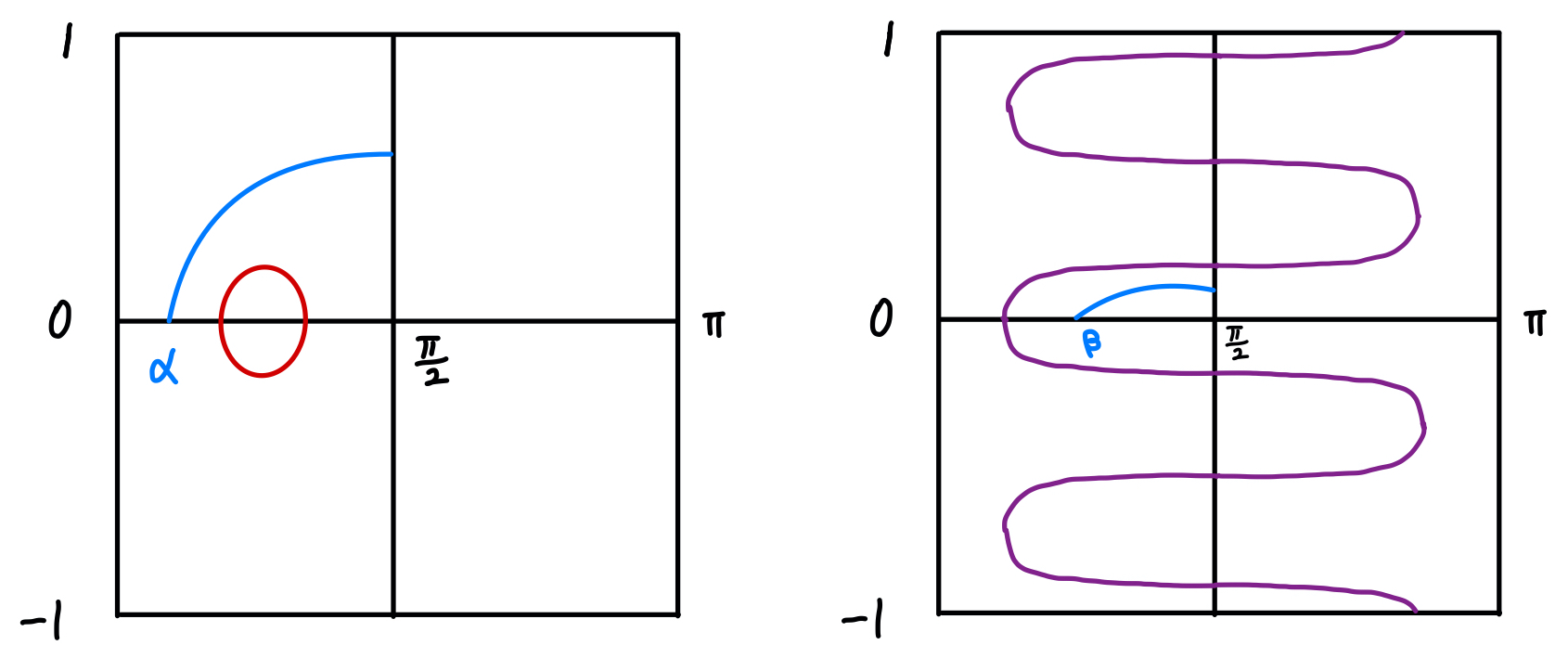
The reflexive symmetry implies that the curve $\gamma_{t}$ intersects the two sides $\{x=0\}$, $\{y=0\}$ orthogonally. We name the intersection point of $\gamma_{t}$ with $\{y=0\}$ as the head point. This curve $\gamma_{t}$ can be expressed as the union of two graphs of smooth functions $u$ and $v$, and we call $u$ the vertical graph function and call its graph as the vertical graph; we call $v$ as the horizontal graph function and call its graph as the horizontal graph. See the picture below for an example.

Let $u_{0}$ and $v_{0}$ be the vertical graph function and the horizontal graph function of the initial curve $\gamma_{0}$. Suppose after reflecting and rotating $\gamma_{0}$ we get a hypersurface $M(0)$ in $S^{n}\times[-1,1]$. Then a family of hypersurfaces $\{M(t)\}_{t\in[0,T)}$ is said to be a mean curvature flow with initial condition $M(0)$ if the corresponding vertical graph function, horizontal graph function $u(\cdot,t)$, $v(\cdot,t)$ of $\gamma_{t}$ satisfy the following equations (see Appendix A):

(2.2)

$$\left\{\begin{aligned} &\frac{\partial u}{\partial t}=\frac{u_{yy}}{1+(u_{y})^{2}}-(n-1)\frac{\cos(u)}{\sin(u)},\\ &\frac{\partial v}{\partial t}=\frac{v_{xx}}{1+(v_{x})^{2}}+(n-1)\frac{\cos x}{\sin x}v_{x},\\ &u(\cdot,0)=u_{0},\ v(\cdot,0)=v_{0},\\ &u_{y}(0,\cdot)=0,\ v_{x}(\frac{\pi}{2},\cdot)=0.\end{aligned}\right.$$

For simplicity, we will say $f(\cdot,t)$ is a solution to equation (2.2) if its corresponding vertical graph function and horizontal graph function solve this equation. We will call the first equation in (2.2) the vertical graph equation, and call the second equation in (2.2) the horizontal graph equation.

Suppose $\gamma^{1}$ and $\gamma^{2}$ are two curves in $D$. We say that $\gamma^{1}$ is on top of $\gamma^{2}$, if for all pairs $(c,y_{1},y_{2})$ such that $(c,y_{1})\in\gamma^{1},(c,y_{2})\in\gamma^{2}$, it holds that $y_{1}\geq y_{2}$. Recall the comparison principle for mean curvature flow:

Therefore, we can use barriers that are either on top of the flow or under the flow at the initial time to control the behavior of the flow at a later time. We will frequently use the following special solutions as barriers in this paper.

Firstly, we consider the static solutions known as the minimal hypersurfaces. The simplest possible examples are the horizontal graphs $(x,v(x,t))$ given by $v(x,t)\equiv C$ for a constant $C\in[-1,1]$. Such a minimal hypersurface is just a section of $S^{n}\times[-1,1]$, and we call it a minimal sphere. There is only one constant vertical graph $(u(y,t),y)$ given by $u(y,t)\equiv\pi/2$. It is the Cartesian product of the geodesic hypersphere in $S^{n}$ with $[-1,1]$, and we still call it a geodesic hypersphere.

Another class of minimal hypersurfaces is the analog of the catenoids, and we call them spherical catenoids. Given a parameter $C\in(0,\pi/2)$, we can solve the ODE

(2.3)

$$\frac{u_{yy}}{1+(u_{y})^{2}}-(n-1)\frac{\cos(u)}{\sin(u)}=0,$$

with initial condition $u(0)=C$ and $u_{y}(0)=0$. First, (2.3) is invariant under $y\leftrightarrow-y$, so the solution must be an even function, and hence we only need to study the part of the solution where $y\geq 0$. It is straightforward to see that $u_{yy}(0)>0$, and hence $u_{y}>0$ in a neighborhood of $0$. Multiplying both sides of (2.3) by $u_{y}$ yields the identity

$$\frac{1}{2}(\log(1+(u_{y})^{2}))_{y}-(n-1)(\log(\sin u))_{y}=0,$$

and then we can conclude that there exists a constant $\lambda_{C}$ such that

$$u_{y}^{2}=\lambda_{C}^{2}(\sin u)^{2(n-1)}-1.$$

By plugging in $u(0)=C$ we obtain

$$\lambda_{C}=(\sin C)^{-(n-1)}.$$

Then we obtain that $u_{y}(y)>0$ for all $y\in(0,Y_{C})$, where $u(Y_{C})=\pi-C$. We may write the expression of $u_{y}$ as

$$u_{y}=\sqrt{\frac{(\sin u)^{2(n-1)}}{(\sin C)^{2(n-1)}}-1}.$$

We can also obtain the information of $u$ by looking at the inverse function $v$, which satisfies the equation

(2.4)

$$\frac{v_{xx}}{1+(v_{x})^{2}}+(n-1)\frac{\cos(x)}{\sin(x)}v_{x}=0,$$

where $v(C)=0$ and $v(\pi-C)=Y_{C}$, and $v_{x}\to\infty$ as $x\searrow C$ or $x\nearrow(\pi-C)$. dividing both sides of (2.4) by $v_{x}$ yields the identity

$$\left[\log(v_{x})-\frac{1}{2}\log(1+(v_{x})^{2})+(n-1)\log\sin x\right]_{x}=0.$$

Therefore, there exists $\bar{\lambda}_{C}>0$ such that

$$\frac{v_{x}}{\sqrt{1+(v_{x})^{2}}}=\bar{\lambda}_{C}(\sin x)^{-(n-1)}.$$

Let $x\searrow C$, we have $\bar{\lambda}_{C}=(\sin C)^{-(n-1)}$. Then we obtain

(2.5)

$$v_{x}=\left(\left(\frac{\sin x}{\sin C}\right)^{2({n-1})}-1\right)^{-1/2}$$

This implies that $v_{x}>0$ for all $x\in(C,\pi-C)$, and $v_{x}(x)+(v(\pi-x))_{x}=0$. Then we can show that $v(x)=2v(\pi/2)-v(\pi-x)$. It is also clear that $v(\pi/2)=Y_{C}/2$.

In fact, the spherical catenoids are periodic in the $\mathbb{R}$ factor, and $Y_{C}$ is half of the period. See Figure 3 for a picture.

In his pioneer work [Ang92], Angenent constructed a rotationally symmetric self-shrinking mean curvature flow in $\mathbb{R}^{n+1}$ that is topological $S^{1}\times S^{n-1}$ before it becomes singular. More precisely, Angenent constructed a closed embedded hypersurface $\Sigma_{n}\subset\mathbb{R}^{n+1}$ that is rotationally symmetric, such that $\{\sqrt{-t}\Sigma_{n}\}_{t<0}$ is a mean curvature flow.

It was observed by Huisken [Hui84] that if $\{\sqrt{-t}\Sigma\}_{t<0}$ is a mean curvature flow, then $\Sigma$ satisfies the equation $\vec{H}+x^{\perp}/2=0$, and such $\Sigma$ is called a shrinker. Moreover, Huisken observed that a shrinker in $\mathbb{R}^{n+1}$ is the critical point of the Gaussian area functional $\mathcal{F}(\Sigma)=\int_{\Sigma}e^{-|x|^{2}/4}d\mathcal{H}^{n}(x)$. Therefore, Angenent reduced the existence of a rotationally symmetric shrinker to the existence of a closed embedded geodesic in the half-plane $\{(x,y)|x\geq 0\}$ equipped with the metric $x^{2(n-1)}e^{-(x^{2}+y^{2})/2}(dx^{2}+dy^{2})$.

Angenent used a shooting method to construct such a closed embedded geodesic. The idea is to examine the trajectory of the geodesics starting from $(r,0)$ with unit tangent vector $(0,1)$ as $r$ varies. Then an interpolation argument asserts the existence of a geodesic trajectory that will get back to some $(s,0)$ again with tangent vector $(0,-1)$. Reflecting this geodesic trajectory along the $x$-axis gives a desired closed embedded geodesic.

We would like to point out that if we replace $(n-1)$ by some $\lambda>0$, all the proofs in [Ang92] still work (See Appendix B for an explanation). We call a closed embedded geodesic in the half-plane $\{(x,y)|x\geq 0\}$ equipped with the metric $x^{2\lambda}e^{-(x^{2}+y^{2})/2}(dx^{2}+dy^{2})$ a $\lambda$-Angenent curve. Such curves will be the barriers. In fact, when $n\geq 3$, we can just use the $(n-1)$-dimensional Angenent torus as the barrier. Only in the case $n=2$ we need a $\lambda$-Angenent curve as the barrier for $\lambda\in(0,1)$.

In this section, we study the solutions to the equation (2.2).

We will introduce the following notations throughout this section. $(M(t))_{t\in[0,T)}$ is a rotationally symmetric mean curvature flow in $S^{n}\times[-1,1]$. The section curve of $M(t)$ is $\gamma_{t}$, and can be expressed as the graph of $f(\cdot,t)$. Therefore $f(\cdot,t)$ is a solution to the equation (2.2). $u(\cdot,t)$, $v(\cdot,t)$ will denote the vertical graph function and the horizontal graph function of $f(\cdot,t)$.

From now on we will assume that the initial section curve $\gamma_{0}$ is ascending. It follows from Proposition 3.1 that $\gamma_{t}$ is an ascending section curve, thus the height of $\gamma_{t}$ (i.e. the maximum of $f(\cdot,t)$) is given by $f(\frac{\pi}{2},t)$. We prove in the next lemma that it is monotone.

Although Lemma 3.2 shows that the height of the section curve of the flow strictly decreases, we do not have a quantitative estimate of the decreasing rate. To obtain such a bound, we need to construct a new family of barriers.

Given $a\in(0,\frac{\pi}{2})$, Consider a smooth function $l_{a}\in C^{\infty}([0,\frac{\pi}{2}])$ such that

$$l_{a}(x)=\left\{\begin{aligned} &0\qquad\text{for}\qquad 0\leq x\leq\frac{a}{2},\\ &1\qquad\text{for}\qquad a\leq x\leq\frac{\pi}{2},\end{aligned}\right.$$

and $l_{a}^{\prime}(x)>0$ for $x\in(\frac{a}{2},a)$.

By similar arguments as in authors’ previous paper [CS23], there exists a smooth solution $L_{a}(x,t)$ to the horizontal graph equation with initial data $L_{a}(x,0)=l_{a}(x)$, and boundary condition $\frac{\partial}{\partial x}L_{a}(0,t)=\frac{\partial}{\partial x}L_{a}(\frac{\pi}{2},t)=0$. We have the following lemmas which are based on the maximum principle and Sturmian theorem (see [CS23, Lemma 3.4, 3.5]).

Next, we examine the behavior of the head point when the singularity appears during the mean curvature flow. By Lemma 3.2, we know the limit of the height $h:=\lim\limits_{t\to T}f(\frac{\pi}{2},t)$ exists. The gradient estimate in Lemma 3.4 implies that if the height of the function $f(\cdot,t)$ tends to $0$, then the head point must tend to the boundary $x=\frac{\pi}{2}$.

On the other hand, if the limit of the height $h$ is not zero, we obtain an improved gradient estimate.

References

• [AAG95] Steven Altschuler, Sigurd B. Angenent, and Yoshikazu Giga. Mean curvature flow through singularities for surfaces of rotation. J. Geom. Anal., 5(3):293–358, 1995.
• [Ama88] Herbert Amann. Dynamic theory of quasilinear parabolic equations. I. Abstract evolution equations. Nonlinear Anal., 12(9):895–919, 1988.
• [Ang92] Sigurd B Angenent. Shrinking doughnuts. In Nonlinear diffusion equations and their equilibrium states, 3, pages 21–38. Springer, 1992.
• [BHH19] Reto Buzano, Robert Haslhofer, and Or Hershkovits. The moduli space of two-convex embedded tori. Int. Math. Res. Not. IMRN, (2):392–406, 2019.
• [BHH21] Reto Buzano, Robert Haslhofer, and Or Hershkovits. The moduli space of two-convex embedded spheres. J. Differential Geom., 118(2):189–221, 2021.
• [BK23] Richard H Bamler and Bruce Kleiner. On the multiplicity one conjecture for mean curvature flows of surfaces. arXiv preprint arXiv:2312.02106, 2023.
• [BM12] Alexander A. Borisenko and Vicente Miquel. Mean curvature flow of graphs in warped products. Trans. Amer. Math. Soc., 364(9):4551–4587, 2012.
• [CH10] Jingyi Chen and Weiyong He. A note on singular time of mean curvature flow. Math. Z., 266(4):921–931, 2010.
• [CS23] Jingwen Chen and Ao Sun. Mean curvature flow with multiplicity 2 convergence. arXiv preprint arXiv:2312.17457, 2023.
• [DN18] Gregory Drugan and Xuan Hien Nguyen. Shrinking doughnuts via variational methods. J. Geom. Anal., 28(4):3725–3746, 2018.
• [ES92] Lawrence C Evans and Joel Spruck. Motion of level sets by mean curvature iii. The Journal of Geometric Analysis, 2(2):121–150, 1992.
• [GLP21] Marco AM Guaraco, Vanderson Lima, and Franco Vargas Pallete. Mean curvature flow in homology and foliations of hyperbolic 33-manifolds. arXiv preprint arXiv:2105.07504, 2021.
• [Gra89] Matthew A. Grayson. Shortening embedded curves. Ann. of Math. (2), 129(1):71–111, 1989.
• [HK19] Robert Haslhofer and Daniel Ketover. Minimal 2-spheres in 3-spheres. Duke Math. J., 168(10):1929–1975, 2019.
• [Hui84] Gerhard Huisken. Flow by mean curvature of convex surfaces into spheres. J. Differential Geom., 20(1):237–266, 1984.
• [HZ23] Sven Hirsch and Jonathan J Zhu. Uniqueness of blowups for forced mean curvature flow. arXiv preprint arXiv:2310.08005, 2023.
• [LSU68] Olga Aleksandrovna Ladyzhenskaia, Vsevolod Alekseevich Solonnikov, and Nina N Ural’tseva. Linear and quasi-linear equations of parabolic type, volume 23. American Mathematical Soc., 1968.
• [Wan02] Mu-Tao Wang. Long-time existence and convergence of graphic mean curvature flow in arbitrary codimension. Invent. Math., 148(3):525–543, 2002.
• [WZ22] Zhichao Wang and Xin Zhou. Min-max minimal hypersurfaces with higher multiplicity. arXiv preprint arXiv:2201.06154, 2022.
• [WZ23] Zhichao Wang and Xin Zhou. Existence of four minimal spheres in S3S^{3} with a bumpy metric. arXiv preprint arXiv:2305.08755, 2023.
• [Zho20] Xin Zhou. On the multiplicity one conjecture in min-max theory. Ann. of Math. (2), 192(3):767–820, 2020.