Mean dimension theory in symbolic dynamics for finitely generated amenable groups ⁰⁰footnotetext: * Corresponding author ⁰⁰footnotetext: 2010 Mathematics Subject Classification: 37B40, 37C85.

Yunping Wang¹, Ercai Chen², Xiaoyao Zhou*²
1 School of Science, Ningbo Unversity of Technology,
Ningbo 315211, Zhejiang, P.R.China
2 School of Mathematical Sciences and Institute of Mathematics, Nanjing Normal University,
Nanjing 210046, Jiangsu, P.R.China
e-mail: yunpingwangj@126.com, ecchen@njnu.edu.cn,
zhouxiaoyaodeyouxian@126.com

Abstract. In this paper, we mainly elucidate a close relationship between the topological entropy and mean dimension theory for actions of polynomial growth groups. We show that metric mean dimension and mean Hausdorff dimension of subshifts with respect to the lower rank subgroup are equal to its topological entropy multiplied by the growth rate of the subgroup. Meanwhile, we also prove the above result holds for the rate distortion dimension of subshifts with respect to the lower rank subgroup and measure entropy. Furthermore, some relevant examples are indicated.

Keywords and phrases: subshift, metric mean dimension, mean Hausdorff dimension, rate distortion dimension, polynomial growth groups.

1 Introduction

Let $(X,G)$ be a $G$ -action topological dynamical system, where $X$ is a compact Hausdorff space and $G$ a topological group. Throughout this paper, $G$ is a finitely generated amenable groups. An important dynamical quantity of a shift is its entropy, which roughly measures the exponential growth rate of its projections on finite sets. For the case $G=\mathbb{N}$ , we consider the one-sided infinite product $A^{\mathbb{N}}$ with the shift map $\sigma:A^{\mathbb{N}}\rightarrow A^{\mathbb{N}}$ defined by

\sigma((x_{n})_{n\in\mathbb{N}})=(x_{n+1})_{n\in\mathbb{N}}.

Define a metric which is compatible with the product topology on $A^{\mathbb{N}}$ as follows: for every $x=(x_{n})_{n\in\mathbb{N}},y=(y_{n})_{n\in\mathbb{N}}\in A^{\mathbb{N}}$ ,

\displaystyle d(x,y)=2^{-\min\left\{n|x_{n}\neq y_{n}\right\}}.

Let $\mathcal{X}$ be a closed invariant subset of $A^{\mathbb{N}}$ . Furstenberg proved the following relationship among entropy, Hausdorff and Minkowski dimensions of $\mathcal{X}$ with respect to $d$ [9, Proposition III.1]:

\displaystyle{\rm dim}_{H}(\mathcal{X},d)={\rm dim}_{M}(\mathcal{X},d)={h_{top}(\mathcal{X},\sigma)},

where $h_{top}(\mathcal{X},\sigma)$ is the topological entropy of $(\mathcal{X},\sigma)$ . Simpson [27] generalized the above results to $\mathbb{Z}^{k}$ action and more general result for amenable group action appears in [8]. For more relevant studies one may refer to [3, 20].

Mean dimension is a conjugacy invariant of topological dynamical systems which was introduced by Gromov [21]. This is a dynamical version of topological dimension and it counts how many parameters per iterate we need to describe an orbit in the dynamical systems. This invariant has several applications which cannot be touched within the framework of topological entropy, see [25, 17, 18]. In particularly, it has many applications to embedding problem whether a dynamical system can be embedded into another or not, see for instance [14, 13, 22, 23, 24].

It is well known that the concepts of entropy and dimension are closely connected. So it is natural to except we can approach to mean dimension from the entropy theory viewpoint. The first attempt of such an approach was made by Lindenstrauss and Weiss [14]. They introduced the notion of metric mean dimension, which is a dynamical analogue of Minkowski dimension [14], and they proved that metric mean dimension is an upper bound of the mean dimension. It allowed them to establish the relationship between the mean dimension and the topological entropy of dynamical systems. Namely, each system with finite topological entropy has zero metric mean dimension and zero mean dimension. Lindenstrauss and Tsukamoto in [15] established a variational principle between the metric mean dimension and the rate distortion function under a mild condition on the metric $d$ (called tame growth of covering numbers, for this definition see [15]). Inspired by the classic variational principle of entropy, they [16] also considered a measure-theoretic notion of mean dimension-rate distortion dimension, which was first introduced by Kawabata and Dembo in [11] and proved a corresponding variational principle for mean dimension. In order to link the measure theoretic aspect of mean dimension theory, they introduced the mean Hausdorff dimension in [16], which is a dynamical analogue of Hausdorff dimension.

Recently, Shinoda and Tsukamoto [26] generalized Furstenberg’s result in [9] to $\mathbb{Z}^{2}$ action which involves metric mean dimension, mean Hausdorff dimension and rate distortion dimension. In this paper, by adopting the method of [26] and [8], we are going to prove the relationship between mean dimension quantities (metric mean dimension, mean Hausdorff dimension and rate distortion dimension) and entropy, which generalize the result of [26] to actions of polynomial growth groups. The main difficulty in carrying out this generalization is that we need a Vitali type covering lemma. To this aim we apply a more general covering lemma developed by Lindentrauss [12].

The paper is organized as follows. In section 2, we review basic definitions of finitely generated amenable groups and mean dimension theory. Meanwhile, we state our main results. In section 3, we introduce covering lemma and give the proof of Theorem 2.1. In section 4, we present the notion of rate distortion dimension and prove the Theorem 2.2 by following Shinoda and Tsukamoto’s technical line. In section 5, we give some examples to illustrate our main theorem.

2 Preliminaries

In this section, we review some of the standard concepts and results on finitely generate amenable groups, metric mean dimension and mean Hausdorff dimension. Finally, we state our main results.

2.1 Finitely generated amenable groups

Let $G$ be an infinite discrete countable group. Let $F(G)$ denote the set of all finite non-empty subset of $G$ . For $K$ , $F\in F(G)$ , let $KF\in F(G)$ , let $KF=\left\{st:s\in K,t\in F\right\}$ and $KF\Delta F=(KF\setminus F)\cup(F\setminus KF)$ . A group $G$ is called amenable if for each $K\in F(G)$ and $\delta>0$ , there exists $F\in F(G)$ such that $|KF\Delta F|<\delta|F|$ , where $|\cdot|$ is the counting measure.

Let $K\in F(G)$ and $\delta>0$ . A finite subset $A\in F(G)$ is called $(K,\delta)$ -invariant if

\dfrac{|B(A,K)|}{|A|}<\delta,

where $B(A,K)$ , the $K$ -boundary of $A$ , is defined by

\displaystyle B(A,K)=\left\{g\in G:Kg\cap A\neq\emptyset~{}\text{and}~{}Kg\cap(G\setminus A)\neq\emptyset\right\}.

Another equivalent condition for the sequence of finite subset $\left\{F_{n}\right\}$ of $G$ to be a F $\phi$ lner sequence is that $\left\{F_{n}\right\}$ becomes more and more invariant, i.e., for each $K\in F(G)$ and $\delta>0$ , $F_{n}$ is $(K,\delta)$ -invariant when $n$ is large enough. A group $G$ is amenable group if and only if $G$ admits a F $\phi$ lner sequence $\left\{F_{n}\right\}$ . For more details and properties of the amenable group, one is referred to [19] [6]. Let $\epsilon\in(0,1)$ . $A_{1},A_{2},\cdots,A_{k}\in F(G)$ are said to be $\epsilon$ -disjoint if there exist mutually disjoint $A_{i}^{\prime}\subset A_{i}$ such that $|A_{i}^{\prime}|\geq(1-\epsilon)|A_{i}|$ for $1\leq i\leq k$ . Recall that a F $\phi$ lner sequence $\left\{F_{n}\right\}$ in $G$ is said to be tempered if there exists a constant $C>0$ which is independent of $n$ such that

\displaystyle|\bigcup\limits_{k<n}F_{k}^{-1}F_{n}|\leq C|F_{n}|,~{}\text{for any}~{}n.

(2.1)

Let $G$ be a finitely generated amenable group with a symmetric generating set $S$ . Recall that a generating set is called symmetric if together with any $s\in S$ it contains $s^{-1}$ . The $S$ -word-length $\ell_{S}(g)$ of an element $g\in G$ is the minimal integer $n\geq 0$ such that $g$ can be expressed as a product of $n$ elements in $S$ , that is,

\displaystyle\ell_{S}(g)=\min\left\{n\geq 0:g=s_{1}\cdots s_{n}:s_{i}\in S,1\leq i\leq n\right\}.

It immediately follows from the definition that for $g\in G$ one has $\ell_{S}(g)=0~{}\text{if an only if}~{}g=1_{G}.$ Define the metric $d_{S}$ on $G$ : $d_{S}(g,h)=\ell_{S}(g^{-1}h).$ It is obvious that the metric $d_{S}$ is invariant by left multiplication.

For $g\in G$ and $n\in\mathbb{N}$ , we denote by

\displaystyle B_{S}^{G}(g,n)=\left\{h\in G:d_{S}(g,h)\leq n\right\},

the ball of radius $n$ in $G$ centered at the element $g\in G$ . When $g=1_{G}$ we have $B_{S}^{G}(1_{G},n)=\left\{h\in G:\ell_{S}(h)\leq n\right\}$ and we simply write $B_{S}^{G}(n)$ instead of $B_{S}^{G}(1_{G},n)$ . Also, when there is no ambiguity on the group $G$ , we omit the subscript $G$ and we simply write $B_{S}(g,n)$ and $B_{S}(n)$ instead of $B_{S}^{G}(g,n)$ and $B_{S}^{G}(n)$ . The growth function of $G$ relative to $S$ is a function $\gamma_{S}:\mathbb{N}\rightarrow\mathbb{N}$ defined by $\gamma_{S}(n)=|B_{S}(n)|=|\left\{g\in G:\ell_{S}(g)\leq n\right\}|.$

Remark 2.1.

[7] Let $G_{1}$ and $G_{2}$ be two finitely generated amenable groups. Then the direct product $G_{1}\times G_{2}$ is also a finitely generated amenable group.

Definition 2.1.

Let $G$ be a finitely generated group of polynomial growth with a symmetric generating set $S$ if there exists constants $d,A,B>0$ such that

An^{d}\leq\gamma_{S}(n)\leq Bn^{d}

for all $n\in\mathbb{N}.$ We denote by ${\rm deg}(G)=d$ the degree of the polynomial growth of $G$ .

In this paper, we consider a finitely generated group of polynomial growth. Polynomial growth groups are amenable. We will review the definitions of metric mean dimension [4] and introduce the mean Hausdorff dimension of amenable group actions in subsection 2.2.

2.2 Metric mean dimension and mean Hausdorff dimension

Let $G$ be a countable discrete amenable group. Let $(\mathcal{X},G)$ be a $G$ -system with $d$ . For $\epsilon>0$ , we define $\#(\mathcal{X},d,\epsilon)$ as the minimum natural number $n$ such that $\mathcal{X}$ can be covered by open sets $U_{1},\cdots,U_{n}$ with ${\rm diam}(U_{i})<\epsilon$ for $1\leq i\leq n$ . For $F\in F(G)$ , define metric $d_{F}$ on $\mathcal{X}$ by

d_{F}(x,y)=\max\limits_{g\in F}d(gx,gy).

For $s\geq 0$ and $\epsilon>0$ , we define $H_{\epsilon}^{s}(\mathcal{X},d)$ as

\displaystyle\inf\left\{\sum\limits_{n=1}^{\infty}({\rm diam}E_{n})^{s}|\mathcal{X}=\bigcup\limits_{n}E_{n}~{}\text{with}~{}{\rm diam}E_{n}<\epsilon~{}\text{for all}~{}n\geq 1\right\}.

(2.2)

We set

{\rm dim}_{H}(\mathcal{X},d,\epsilon)=\sup\left\{s\geq 0|H_{\epsilon}^{s}(\mathcal{X},d)\geq 1\right\}.

The Hausdorff dimension ${\rm dim}_{H}(\mathcal{X},d)$ is given by

{\rm dim}_{H}(\mathcal{X},d)=\lim\limits_{\epsilon\rightarrow 0}{\rm dim}_{H}(\mathcal{X},d,\epsilon).

We define the upper and lower mean Hausdorff dimension. Let $\left\{F_{n}\right\}$ be a F $\phi$ lner sequence in $G$ , we can define

	$\displaystyle\overline{\rm mdim}_{H}(\mathcal{X},\left\{F_{n}\right\},d)=\lim\limits_{\epsilon\rightarrow 0}\left(\limsup\limits_{n\rightarrow\infty}\dfrac{{\rm dim}_{H}(\mathcal{X},d_{F_{n}},\epsilon)}{\|F_{n}\|}\right),$
	$\displaystyle\underline{\rm mdim}_{H}(\mathcal{X},\left\{F_{n}\right\},d)=\lim\limits_{\epsilon\rightarrow 0}\left(\liminf\limits_{n\rightarrow\infty}\dfrac{{\rm dim}_{H}(\mathcal{X},d_{F_{n}},\epsilon)}{\|F_{n}\|}\right).$

When these two quantities are equal to each other, we denote the common value by ${\rm mdim}_{H}(\mathcal{X},\left\{F_{n}\right\},d)$ . For any $\epsilon>0$ , we define

S(\mathcal{X},G,d,\epsilon)=\lim\limits_{n\rightarrow\infty}\dfrac{1}{|F_{n}|}\log\#(\mathcal{X},d_{F_{n}},\epsilon).

The limit always exists and does not depend on the choice of the F $\phi$ lner sequence $\left\{F_{n}\right\}$ . The upper and lower metric mean dimension is then defined by

\overline{\rm mdim}_{M}(\mathcal{X},G,d)=\limsup\limits_{\epsilon\rightarrow 0}\dfrac{S(\mathcal{X},G,d,\epsilon)}{|\log\epsilon|},

\underline{\rm mdim}_{M}(\mathcal{X},G,d)=\liminf\limits_{\epsilon\rightarrow 0}\dfrac{S(\mathcal{X},G,d,\epsilon)}{|\log\epsilon|}.

When the upper and lower limits coincide, we denote the common value by ${\rm midm}_{M}(\mathcal{X},G,d)$ .

The following result is the dynamical analogue of the fact that Minkowski dimension no less than Hausdorff dimension.

Proposition 2.1.

Let $\left\{F_{n}\right\}$ be a F $\phi$ lner sequence, then

\displaystyle\overline{{\rm mdim}}_{H}(\mathcal{X},\left\{F_{n}\right\},d)\leq\underline{{\rm mdim}}_{M}(\mathcal{X},G,d).

Proof.

Let $\left\{F_{n}\right\}$ be a the F $\phi$ lner sequence in $G$ . For $n\geq 0$ , $\epsilon>0$ , choose an open cover $\mathcal{X}=U_{1}\cup\cdots\cup U_{m}$ with ${\rm diam}(U_{i},d_{F_{n}})\leq\epsilon$ and $m=\#(\mathcal{X},d_{F_{n}},\epsilon)$ . We have

H_{\epsilon}^{s}(\mathcal{X},d_{F_{n}})\leq m\epsilon^{s}.

If $s>\log m/\log(1/\epsilon)$ , then $H^{s}(\mathcal{X},d_{F_{n}})<1$ . This shows

{\rm dim}_{H}(\mathcal{X},d_{F_{n}},\epsilon)\leq\dfrac{\log\#(\mathcal{X},d_{F_{n}},\epsilon)}{\log(1/\epsilon)}.

Divide this by $|F_{n}|$ and take limits with respect to $n$ and then $\epsilon$ . It follows that $\overline{\rm mdim}_{H}(\mathcal{X},\left\{F_{n}\right\},d)\leq\underline{\rm midm}_{M}(\mathcal{X},G,d).$ ∎

2.3 Statement of the main results

Now we state the main theorems. Let $G_{1}$ and $G_{2}$ be finitely generated groups of polynomial growth. Then direct product $G=G_{1}\times G_{2}$ is also finitely generated of polynomial growth. Let $S_{1}$ and $S_{2}$ be finite symmetric generating subsets of $G_{1}$ and $G_{2}$ . Then the set

S=(S_{1}\times\left\{1_{G_{1}}\right\})\cup(\left\{1_{G_{2}}\right\}\times S_{2})

is a finite symmetric generating subset of $G$ . We denote by ${\rm deg}(G_{1})$ and ${\rm deg}(G_{2})$ the degrees of the polynoimal growth of $G_{1}$ and $G_{2}$ , respectively (e.g., ${\rm deg}(\mathbb{Z}^{k})=k$ ). Set $S=\left\{s_{1},\cdots s_{m}\right\}$ . Next we defines a order in $S$ which formalize through the following construction: given $s_{i},s_{j}\in S$ we say that $s_{i}<s_{j}$ if $i<j$ . Hence $s_{1}<s_{2}<\cdots<s_{m}$ . Hence we can consider the order in $G$ . For $g,g^{\prime}\in G$ , we call $g<g^{\prime}$ if $\ell(g)<\ell(g^{\prime})$ . If $\ell(g)=\ell(g^{\prime})=n$ , then there exist $s_{1},\cdots,s_{n}$ and $s_{1}^{\prime},\cdots,s_{n}^{\prime}$ such that

\displaystyle g=s_{1}\cdots s_{n},~{}g^{\prime}=s_{1}^{\prime}\cdots s_{n}^{\prime}.

Take $k=\min\left\{i:s_{i}\neq s_{i}^{\prime}\right\}$ . When $s_{k}<s_{k}^{\prime}$ , we denote by $g<g^{\prime}$ , otherwise, $g>g^{\prime}$ . Then we can arrange the elements in the group. Let $G=(g_{n})_{n=0}^{\infty}$ be an enumeration of $G$ according to the order such that $\ell(1_{G})=\ell_{S}(g_{0})\leq\ell_{S}(g_{1}))\leq\ell_{S}(g_{2})\cdots$ .

We can define a metric $d$ on $A^{G}$ by the following:

\displaystyle d(x,y)=2^{-\min\left\{|g_{n}|_{\infty}\big{|}x_{g_{n}}\neq y_{g_{n}}\right\}},

(2.3)

where $|g_{n}|_{\infty}=\max\left\{\ell_{S_{1}}(g_{n,1}),\ell_{S_{2}}(g_{n,2})\right\}$ and $g=(g_{n,1},g_{n,2})$ . A closed $G$ -invariant subset $\mathcal{X}$ of $A^{G}$ is called a subshift of $A^{G}$ .

Theorem 2.1.

Let $\mathcal{X}\subset A^{G}$ be a subshift. Suppose that ${\rm deg}(G_{2})=1$ . Then

(1).

$\overline{\rm mdim}_{M}(\mathcal{X},{G_{1}},d)\leq c_{1}\cdot h_{top}(\mathcal{X},{G}),$ where $c_{1}=\limsup\limits_{n\rightarrow\infty}\frac{|B_{S_{2}}(n)|}{n}$ .
(2).

$\underline{{\rm mdim}}_{H}(\mathcal{X},\left\{B_{S_{1}}(n)\right\},d)\geq c_{2}\cdot h_{top}(\mathcal{X},G),$ where $c_{2}=\liminf\limits_{n\rightarrow\infty}\frac{|B_{S_{2}}(n)|}{n}.$

In particular, if $c_{1}=c_{2}=c$ , we have

\displaystyle{\rm mdim}_{H}(\mathcal{X},\left\{B_{S_{1}}(n)\right\},d)={\rm mdim}_{M}(\mathcal{X},{G_{1}},d)=c\cdot h_{top}(\mathcal{X},{G}).

Theorem 2.2.

If $\mu$ is a Borel probability measure on $\mathcal{X}$ invariant under both $\sigma_{1}$ and $\sigma_{2}$ and $c_{1}=c_{2}=c$ , then

\displaystyle{\rm rdim}(\mathcal{X},\sigma_{1},\left\{B_{S_{1}}(n)\right\},d,\mu)=c\cdot h_{\mu}(\mathcal{X},G).

Remark 2.2.

(1)

It is not clear whether the value of $c$ exists for general amenable groups. Hence we only consider the polynomial growth groups in this paper.
(2)

The reason for imposing the condition ${\rm deg}(G_{2})=1$ is that if ${\rm deg}(G_{2})>1$ , we don’t know whether the value of $c$ exists.

3 Proof of Theorem 2.1

For a finite alphabet $A$ and a finitely generated group of polynomial growth $G$ , the full $G$ -shift over $A$ is the set $A^{G}$ , which is viewed as a compact topological space with the discrete product topology. Consider the shift action on the product space $A^{G}$ :

g^{\prime}(x_{g})_{g\in G}=(x_{gg^{\prime}})_{g\in G},\text{for all}~{}g^{\prime}\in G~{}\text{and }~{}(x_{g})_{g\in G}\in A^{G}.

We define the shifts $\sigma_{1}$ and $\sigma_{2}$ on $A^{G}$ by $(\sigma_{1,g}x)_{(g_{1},g_{2})}=x_{(g_{1}g,g_{2})}$ and $(\sigma_{2,h}x)_{(g_{1},g_{2})}=x_{(g_{1},g_{2}h)}$ for all $g\in G_{1}$ , $h\in G_{2}$ , $(g_{1},g_{2})\in G$ . Let $\mathcal{X}$ be a subshift. For $E\subset G$ , let $\pi_{E}:\mathcal{X}\rightarrow A^{E}$ denote the canonical projection map, that is, the map defined by $\pi_{E}(x):=x|_{E}$ for all $x\in\mathcal{X}$ , where $x|_{E}$ denote the restriction of $x:G\rightarrow A$ to $E\subset G$ . For each finite set $F\subset G$ and $\omega\in A^{F}$ , a subset $C\subset\mathcal{X}$ is called a cylinder over $F$ if there exists $x\in\mathcal{X}$ such that $C$ is equal to the set of all $x\in\mathcal{X}$ with $\pi_{F}(x)=\pi_{F}(y)$ . The proof falls naturally into two steps.

Step 1: $\overline{\rm mdim}_{M}(\mathcal{X},G_{1},d)\leq c_{1}\cdot h_{top}(\mathcal{X},G).$

Proof.

For $\epsilon>0$ , choose $M>0$ such that $2^{-M}<\epsilon<2^{-M+1}$ . For each a natural number $N>0$ , then

\displaystyle\#(\mathcal{X},d_{B_{S_{1}}(N)}^{\sigma_{{1}}},\epsilon)\leq|\pi_{(B_{S_{1}}(M)B_{S_{1}}(N)\times B_{S_{2}}(M))}(\mathcal{X})|,

where $d_{B_{S_{1}}(N)}^{\sigma_{1}}(x,y)=\max_{g\in B_{S_{1}}(N)}d(\sigma_{1,g}x,\sigma_{1,g}y)$ . Since $M-1\leq\log(1/\epsilon)\leq M$ ,

		$\displaystyle\overline{\rm mdim}_{M}(\mathcal{X},G_{1},d)$
	$\displaystyle=$	$\displaystyle\limsup\limits_{\epsilon\rightarrow 0}\left(\lim\limits_{N\rightarrow\infty}\dfrac{\log\#(\mathcal{X},d_{B_{S_{1}}(N)}^{\sigma_{{1}}},\epsilon)}{\|B_{S_{1}}(N)\|\log(1/\epsilon)}\right)$
	$\displaystyle\leq$	$\displaystyle\lim\limits_{M\rightarrow\infty}\left(\lim\limits_{N\rightarrow\infty}\dfrac{\|\pi_{(B_{S_{1}}({M})B_{S_{1}}(N)\times B_{S_{2}}({M}))}(\mathcal{X})\|}{\|B_{S_{1}}(N)\|({M-1})}\right)$
	$\displaystyle\leq$	$\displaystyle\lim\limits_{M\rightarrow\infty}\left(\lim\limits_{N\rightarrow\infty}\dfrac{\|\pi_{(B_{S_{1}}({M})B_{S_{1}}(N)\times B_{S_{2}}({M}))}(\mathcal{X})\|}{\|B_{S_{1}}({M})B_{S_{1}}(N)\|\|B_{S_{2}}({M})\|}\times\dfrac{\|B_{S_{1}}({M})B_{S_{1}}(N)\|\|B_{S_{2}}({M})\|}{\|B_{S_{1}}(N)\|({M-1})}\right)$

Since $\left\{B_{S_{1}}(N)\right\}$ is a F $\phi$ lner sequence, then $\lim\limits_{N\rightarrow\infty}\dfrac{|B_{S_{1}}({M})B_{S_{1}}(N)|}{|B_{S_{1}}(N)|}=1$ . Note that $\limsup\limits_{M\rightarrow\infty}\dfrac{|B_{S_{2}}(M)|}{{M}}=c_{1}$ . We can get the desired result. ∎

We next give the following covering lemma which was proved by Linedentrauss [12]. This lemma is crucial in the proof of step 2 of Theorem 2.1.

Lemma 3.1.

[12] For any $\delta\in(0,1/100)$ , $C>0$ and finite $D\subset G$ , let $M\in\mathbb{N}$ be sufficiently large (depending only on $\delta$ , $C$ and $D$ ). Let $F_{i,j}$ be an array of a finite subsets of $G$ where $i=1,\cdots,M$ and $j=1,\cdots,\ell_{i}$ , such that

•

For every $i$ , $\overline{F}_{i,*}=\left\{F_{i,j}\right\}_{j=1}^{\ell_{i}}$ satisfies

$\displaystyle|\bigcup\limits_{k^{\prime}<k}F_{i,k^{\prime}}^{-1}F_{i,k}|\leq C|F_{i,k}|,\text{for}~{}k=2,\cdots,\ell_{i}.$

Denote $F_{i,*}=\bigcup\overline{F}_{i,*}$ .
•

The finite set sequence $F_{i,*}$ satisfy that for every $1\leq i\leq M$ and every $1\leq k\leq\ell_{i}$ ,

$\displaystyle|\bigcup\limits_{i^{\prime}<i}DF_{i^{\prime},*}^{-1}F_{i,k}|\leq(1+\delta)|F_{i,k}|.$

Assume that $A_{i,j}$ is another array of finite subset of $G$ with $F_{i,j}A_{i,j}\subset F$ for some finite subset $F$ of $G$ . Let $A_{i,*}=\cup_{j}A_{i,j}$ and

\displaystyle\alpha=\dfrac{\min\limits_{1\leq i\leq M}|DA_{i,*}|}{|F|}.

Then the collection of subsets of $F$ ,

\displaystyle\overline{F}=\left\{F_{i,j}a:1\leq i\leq M,1\leq j\leq\ell_{i}~{}\text{and}~{}a\in A_{i,j}\right\}

has a subfamily $\mathcal{F}$ that is $10\delta^{1/4}$ -disjoint such that

\displaystyle|\cup\mathcal{F}|\geq(\alpha-\delta^{1/4})|F|.

Step 2: $\underline{{\rm mdim}}_{H}(\mathcal{X},\left\{B_{S_{1}}(N)\right\},d)\geq c_{2}\cdot h_{top}(\mathcal{X},G)$ .

Proof.

Set $s=c_{2}\cdot h_{top}(\mathcal{X},G),~{}h=h_{top}(\mathcal{X},G).$ We suppose $\underline{\rm mdim}_{H}(\mathcal{X},\left\{B_{S_{1}}(n)\right\},d)<s$ . We would like to get a contradiction. Take $\epsilon$ such that $s\epsilon-\frac{\epsilon^{2}}{2}<1$ and

\displaystyle\underline{\rm mdim}_{H}(\mathcal{X},\left\{B_{S_{1}}(n)\right\},d)<s-(h+2)\epsilon.

Let $D=\left\{e_{G}\right\}\subset G$ and $C>0$ be the constant in the tempered condition for the F $\phi$ lner sequence $\left\{B_{S}(n)\right\}$ . We choose $0<\delta<\min\left\{1/100,\epsilon\right\}$ small enough and a natural number $M$ satisfying the following conditions:

\displaystyle H(\delta)+\delta\log M<\epsilon^{3}/4c_{2},~{}|A|^{\delta}<2^{\epsilon^{3}/4c_{2}},~{}1/(1-10\delta^{1/4})<1+\epsilon^{2}.

(3.1)

Here $H(\delta)=-\delta\log\delta-(1-\delta)\log(1-\delta)$ . (Recall that the base of the logarithm is two.) Take $M\approx\log C/\delta^{2}$ to satisfy the requirement of Lemma 3.1 corresponding to $\delta,D$ and $C$ . Then we can choose a sufficiently small $\delta$ satisfying the second and third conditions.

We choose a natural number $r_{0}$ such that

\displaystyle r_{0}>\dfrac{1}{\delta(1-10\delta^{1/4})}.

(3.2)

and

\displaystyle(s-(h+2)\epsilon)r<(s-(h+1)\epsilon)(r-1),~{}~{}|B_{S_{2}}(r)|>r(c_{2}-\epsilon)

(3.3)

for every $r\geq r_{0}$ .

From $\underline{\rm mdim}_{H}(\mathcal{X},\left\{B_{S_{1}}(N)\right\},d)<s-(h+2)\epsilon$ , for each $i=1,2,\cdots M$ , we can find $N_{i}>0$ satisfying

\displaystyle\dfrac{1}{|B_{S_{1}}(N_{i})|}{\rm dim}_{H}(\mathcal{X},d_{B_{S_{1}}(N_{i})}^{\sigma_{1}},2^{-r_{0}})<s-(h+2)\epsilon.

Also, we let the sequence $\left\{N_{i}\right\}$ be increasing. This implies that there exists a covering $\mathcal{X}=\cup_{j=1}^{l_{i}}E_{j}^{i}$ satisfying

\displaystyle{\rm diam}(E_{j}^{i},d_{B_{S_{1}}(N_{i})}^{\sigma_{1}})<2^{-r_{0}}(1\leq j\leq l_{i}),\sum_{j=1}^{l_{i}}({\rm diam}(E_{j}^{i},~{}d_{B_{S_{1}}(N_{i})}^{\sigma_{1}}))^{(s-(h+2)\epsilon)|B_{S_{1}}(N_{i})|}<1.

Set $2^{-r_{j}^{i}}={\rm diam}(E_{j}^{i},d_{A_{N_{i}}}^{\sigma_{1}}).$ Then $r_{j}^{i}$ is a natural number with $r_{j}^{i}>r_{0}$ . Choose $x_{j}^{i}\in E_{j}^{i}$ , let $C_{j}^{i}=\pi_{F_{n_{i,j}}}^{-1}\left(\pi_{F_{n_{i,j}}}(x_{j}^{i})\right)$ be a cylinder over

F_{n_{i,j}}:=\left\{B_{S_{1}}(r_{j}^{i}-1)B_{S_{1}}(N_{i})\times B_{S_{2}}(r_{j}^{i}-1)\right\}.

Then $E_{j}^{i}\subset C_{j}^{i}$ and $\mathcal{X}=\cup_{j=1}^{\ell_{i}}C_{j}^{i}$ . For each $1\leq i\leq M$ , we can get $\{F_{n_{i,1}},\cdots,F_{n_{i,l_{i}}}\}$ . Without loss of generality, let $r_{1}^{i}<r_{2}^{i}<\cdots<r_{l_{i}}^{i}$ . Then let $\left\{F_{i,1},\cdots,F_{i,l_{i}}\right\}$ in Lemma 3.1 be as

\displaystyle\left\{F_{i,1},\cdots,F_{i,l_{i}}\right\}=\{F_{n_{i,1}},\cdots,F_{n_{i,l_{i}}}\}.

Since $|B_{S_{2}}(r)|>r(c_{2}-\epsilon)$ and $s-(h+1)\epsilon<(s-\epsilon)\frac{c_{2}-\epsilon}{c_{2}}$ , we have

\displaystyle|F_{i,j}|=|B_{S_{1}}(r_{j}^{i}-1)B_{S_{1}}(N_{i})\times B_{S_{2}}(r_{j}^{i}-1)|\geq|B_{S_{1}}(N_{i})||B_{S_{2}}(r_{j}^{i}-1)|,

and

	$\displaystyle\dfrac{1}{c_{2}}(s-\epsilon)\|F_{i,j}\|$	$\displaystyle\geq\dfrac{1}{c_{2}}(s-\epsilon)\|B_{S_{1}}((N_{i})\|\|B_{S_{2}}(r_{j}^{i}-1)\|$
		$\displaystyle>(s-\epsilon)\|B_{S_{1}}((N_{i})\|\left(\frac{(r_{j}^{i}-1)(c_{2}-\epsilon)}{c_{2}}\right)$
		$\displaystyle>(s-(h+1)\epsilon)\|B_{S_{1}}(N_{i})\|(r_{j}^{i}-1)$
		$\displaystyle>(s-(h+2)\epsilon)\|B_{S_{1}}(N_{i})\|r_{j}^{i}.~{}~{}(\text{by}~{}\ref{cd})$

Hence

\displaystyle 2^{-\frac{1}{c_{2}}(s-\epsilon)|F_{i,j}|}<2^{-(s-(h+2)\epsilon)|B_{S_{1}}(N_{i})|r_{j}^{i}}={\rm diam}(E_{j}^{i},d_{B_{S_{1}}(N_{i})}^{\sigma_{1}})^{(s-(h+2)\epsilon)|B_{S_{1}}(N_{i})|}.

It follows that

\displaystyle\sum\limits_{j=1}^{l_{i}}2^{-\frac{1}{c_{2}}(s-\epsilon)|F_{i,j}|}\leq\sum\limits_{j=1}^{l_{i}}({\rm diam}(E_{j}^{i},~{}d_{A_{N_{i}}}^{\sigma_{1}}))^{(s-(h+2)\epsilon)|B_{S_{1}}(N_{i})|}<1.

(3.4)

For any $x\in\mathcal{X}$ and sufficiently large $N$ (independent on $x$ ), let

\displaystyle A_{i,j}=\left\{a\in B_{S}(N):F_{i,j}a\subset B_{S}(N)~{}\text{and}~{}\sigma^{a}x\in C_{j}^{i}\right\}.

We note here that $A_{i,j}$ depends on $x$ . For any $g\in B_{S}(N)\setminus B(B_{S}(N),F_{i,*})$ , we have $F_{i,*}g\subset B_{S}(N)$ . Then $F_{i,j}g\subset B_{S}(N)$ for each $1\leq j\leq l_{i}$ . Since $\left\{C_{j}^{i}\right\}_{j=1}^{l_{i}}$ cover $\mathcal{X}$ , there exists $C_{j}^{i}$ such that $\sigma^{g}x\in C_{j}^{i}$ . This implies $g\in A_{i,j}$ and $B_{S}(N)\setminus B(B_{S}(N),F_{i,*})\subset A_{i,*}$ . Let $N$ be sufficiently large so that $B_{S}(N)$ is $(F_{i,*},\delta)$ -invariant for all $1\leq i\leq M$ , $1\leq j\leq l_{i}$ , then

\displaystyle\alpha=\dfrac{\min_{1\leq i\leq M}|DA_{i,*}|}{|B_{S}(N)|}>1-\delta.

We note that the array $\left\{F_{i,j}\right\}$ meet the first requirement in Lemma 3.1 because of the tempered condition of $\left\{B_{S}(N)\right\}$ . For the second requirement, we need to choose $N_{i}$ large enough compared with $r_{l_{i-1}}^{i-1}$ for every $2\leq i\leq M$ . Now we can apply Lemma 3.1 to

\overline{\mathcal{F}}=\left\{F_{i,j}a:1\leq i\leq M,1\leq j\leq l_{i}~{}\text{and}~{}a\in A_{i,j}\right\},

we can find a subcollection $\mathcal{F}$ that is $10\delta^{1/4}$ -disjoint such that

\displaystyle|\cup\mathcal{F}|\geq(1-\delta-\delta^{1/4})|B_{S}(N)|.

(3.5)

The element in $\mathcal{F}$ will be denoted by $F_{i,j}a$ . Denote by $\overline{A}$ the collection of $a$ ’s such that $F_{i,j}a$ occurs in $\mathcal{F}$ . The cardinality of $\overline{A}$ is no more than the cardinality of the subcollection $\mathcal{F}$ . Then $|\overline{A}|\leq|\mathcal{F}|$ . Note that $\mathcal{F}$ is $10\delta^{1/4}$ -disjoint, we have

\displaystyle\sum\limits_{F_{i,j}a\in\mathcal{F}}|F_{i,j}a|\leq\dfrac{1}{1-10\delta^{1/4}}|\cup\mathcal{F}|\leq\dfrac{1}{1-10\delta^{1/4}}|B_{S}(N)|.

Then

\displaystyle|\overline{A}|\leq|\mathcal{F}|\leq\dfrac{1}{\min{|F_{i,j}|}}\cdot\dfrac{1}{1-10\delta^{1/4}}|B_{S}(N)|\leq\delta|B_{S}(N)|.~{}~{}(\text{by}~{}(\ref{1}))

Set

\displaystyle D(x)=\left\{(a,i,j):a\in A_{i,j}~{}1\leq i\leq M,~{}1\leq j\leq\ell_{i}~{}\text{such that}~{}F_{i,j}a\in\mathcal{F}\right\}.

By the above argument, if $N>0$ is sufficiently large, we have the following conclusion:

(1)

For each $(a,i,j)\in D(x)$ , we have $\sigma^{a}x\in C_{j}^{i}$ and $F_{i,j}a\subset\mathcal{F}$ .
(2)

If $(a,i,j)$ and $(a^{\prime},i^{\prime},j^{\prime})$ are two different element of $D(x)$ , then $F_{i,j,}a$ and $F_{i^{\prime},j^{\prime}}a^{\prime}$ is $10\delta^{1/4}$ disjoint.
(3)

$|\bigcup\limits_{(a,i,j)\in D(x)}F_{i,j}a|\geq(1-\delta-\delta^{1/4})|B_{S}(N)|$ .

For each $x\in\mathcal{X}$ we define $\underline{D}(x)\subset B_{S}(N)\times[1,M]$ as the set of $(a,i)$ such that there exists $j\in[1,\ell_{i}]$ with $(a,i,j)\in D(x)$ . (Note that the sets $D(x)$ and $\underline{D}(x)$ depend on $N$ ). For simplicity of notation, we write $D(x)$ and $\underline{D}(x)$ instead of $D_{N}(x)$ and $\underline{D}_{N}(x)$ .

Claim 1.

If $N$ is sufficiently large then the number of possibilities of $\underline{D}(x)$ is bounded as follows:

\displaystyle|\left\{\underline{D}(x)|x\in\mathcal{X}\right\}|<2^{(\epsilon^{3}/4c_{2})|B_{S}(N)|}.

Proof.

It is well-known that

\tbinom{n}{k}\leq 2^{nH(k/n)}.

Since $|\overline{A}|\leq\delta|B_{S}(N)|$ , then the number of possibilities of $\underline{D}(x)$ is bounded by

	$\displaystyle\sum\limits_{k=1}^{\delta\|B_{S}(N)\|}\tbinom{\|B_{S}(N)\|}{k}\times M^{\delta\|B_{S}(N)\|}$	$\displaystyle\leq\|B_{S}(N)\|\cdot 2^{\|B_{S}(N)\|H(\delta)}\times 2^{\|B_{S}(N)\|\delta\log M}$
		$\displaystyle=\|B_{S}(N)\|\cdot 2^{\|B_{S}(N)\|(H(\delta)+\delta\log M)}.$

We assume $H(\delta)+\delta\log M<(\epsilon^{3}/4c_{2})$ in (3.1). Hence, if $N$ is sufficiently large then

\displaystyle|B_{S}(N)|\cdot 2^{|B_{S}(N)|(H(\delta)+\delta\log M)}<2^{(\epsilon^{3}/4c_{2})|B_{S}(N)|}.

∎

Take a subset $E\subset B_{S}(N)\times[1,M]$ such that there exists $x\in\mathcal{X}$ with $\underline{D}(x)=E$ . We denote by $\mathcal{X}_{E}$ the set of $x\in\mathcal{X}$ with $\underline{D}(x)=E$ . Let $E=\left\{(a_{1},i_{1}),(a_{2},i_{2}),\cdots,(a_{k},i_{k})\right\}$ .

Claim 2.

\displaystyle|\pi_{B_{S}(N)}(\mathcal{X}_{E})|\cdot 2^{-\frac{1}{c_{2}}(s-\epsilon)(1+\epsilon^{2})|B_{S}(N)|}\leq|A|^{(\delta+\delta^{1/4})|B_{S}(N)|}.

Proof.

For ${\bf j}=(j_{1},\cdots,j_{k})\in[1,\ell_{i_{1}}]\times\cdots\times[1,\ell_{i_{k}}]$ , we denote by $\mathcal{X}_{E,{\bf j}}\subset\mathcal{X}_{E}$ the set of $x\in\mathcal{X}_{E}$ with $D(x)=\left\{(a_{1},i_{1},j_{1}),\cdots,(a_{k},i_{k},j_{k})\right\}$ . We have $\sigma^{a_{m}}(x)\in C_{j_{m}}^{i_{m}}$ for $x\in\mathcal{X}_{E,{\bf j}}$ . Therefore we have

\displaystyle|\pi_{B_{S}(N)}(\mathcal{X}_{E,{\bf j}})|\leq|A|^{(\delta+\delta^{1/4})|B_{S}(N)|}.

Here the inequality follows from (3.5). This follows from

	$\displaystyle\|\pi_{B_{S}(N)}(\mathcal{X}_{E})\|\cdot 2^{-\frac{1}{c_{2}}(s-\epsilon)(1+\epsilon^{2})\|B_{S}(N)\|}$	$\displaystyle=\sum\limits_{{\bf j}}\|\pi_{B_{S}(N)}(\mathcal{X}_{E,\bf j})\|\cdot 2^{-\frac{1}{c_{2}}(s-\epsilon)(1+\epsilon^{2})\|B_{S}(N)\|}$
		$\displaystyle\leq\sum\limits_{{\bf j}}\|A\|^{(\delta+\delta^{1/4})\|B_{S}(N)\|}2^{-\frac{1}{c_{2}}(s-\epsilon)(1+\epsilon^{2})\|B_{S}(N)\|}.$

Take ${\bf j}=(j_{1},\cdots,j_{k})\in[1,\ell_{i_{1}}]\times\cdots\times[1,\ell_{i_{k}}]$ with $\mathcal{X}_{E,{\bf j}}\neq\emptyset$ . Since

\displaystyle\sum\limits_{F_{i,j}a\in\mathcal{F}}|F_{i,j}a|\leq\dfrac{1}{1-10\delta^{1/4}}|B_{S}(N)|<(1+\epsilon^{2})|B_{S}(N)|~{}\text{by}~{}(\ref{da}),

we have

\displaystyle 2^{-\frac{1}{c_{2}}(s-\epsilon)(1+\epsilon^{2})|B_{S}(N)|}\leq\prod_{m=1}^{k}2^{-\frac{1}{c_{2}}(s-\epsilon)|F_{i_{m},j_{m}}|}.

Moreover

\displaystyle|\pi_{B_{S}(N)}(\mathcal{X}_{E})|\cdot 2^{-\frac{1}{c_{2}}(s-\epsilon)(1+\epsilon^{2})|B_{S}(N)|}\leq\sum\limits_{{\bf j}}|A|^{(\delta+\delta^{1/4})|B_{S}(N)|}\prod_{m=1}^{k}2^{-\frac{1}{c_{2}}(s-\epsilon)|F_{i_{m},j_{m}}|}.

The right-hand side isn’t more than

\displaystyle|A|^{(\delta+\delta^{1/4})|B_{S}(N)|}\left(\sum\limits_{j=1}^{l_{i_{1}}}2^{-\frac{1}{c_{2}}(s-\epsilon)|F_{i_{1},j}|}\right)\times\cdots\times\left(\sum\limits_{j=1}^{l_{i_{k}}}2^{-\frac{1}{c_{2}}(s-\epsilon)|F_{i_{k},j}|}\right).

According to (3.4), we have

\displaystyle|\pi_{B_{S}(N)}(\mathcal{X}_{E})|\cdot 2^{-\frac{1}{c_{2}}(s-\epsilon)(1+\epsilon^{2})|B_{S}(N)|}\leq|A|^{(\delta+\delta^{1/4})|B_{S}(N)|}.

∎

We can now proceed to prove Theorem 2.1.

	$\displaystyle\|\pi_{B_{S}(N)}(\mathcal{X}_{E})\|\cdot 2^{-\frac{1}{c_{2}}(s-\epsilon)(1+\epsilon^{2})\|B_{S}(N)\|}$	$\displaystyle\leq\|A\|^{(\delta+\delta^{1/4})\|B_{S}(N)\|}$
		$\displaystyle\leq 2^{\|B_{S}(N)\|\epsilon^{3}/4c_{2}}.~{}\text{by}~{}(\ref{da})$

If $N$ is sufficiently large, the number of choices $E\subset B_{S}(N)\times[1,M]$ such that $\mathcal{X}_{E}\neq\emptyset$ is not greater than $2^{(\epsilon^{3}/4c_{2})|B_{S}(N)|}$ . Hence

	$\displaystyle\|\pi_{B_{S}(N)}(\mathcal{X})\|\cdot 2^{-\frac{1}{c_{2}}(s-\epsilon)(1+\epsilon^{2})\|B_{S}(N)\|}$	$\displaystyle=\sum\limits_{E~{}\text{with}~{}\mathcal{X}_{E}\neq\emptyset}\|\pi_{B_{S}(N)}(\mathcal{X}_{E})\|\cdot 2^{-\frac{1}{c_{2}}(s-\epsilon)(1+\epsilon^{2})\|B_{S}(N)\|}$
		$\displaystyle<2^{(\epsilon^{3}/4c_{2})\|B_{S}(N)\|}\times 2^{(\epsilon^{3}/4c_{2})\|B_{S}(N)\|}$
		$\displaystyle=2^{(\epsilon^{3}/2c_{2})\|B_{S}(N)\|}.$

Then

\displaystyle\dfrac{\log|\pi_{B_{S}(N)}(\mathcal{X})|}{|B_{S}(N)|}<\dfrac{1}{c_{2}}(s-\epsilon+s\epsilon^{2}-\frac{1}{2}\epsilon^{3}).

Letting $N\rightarrow\infty$ , we have

\displaystyle h_{top}(\mathcal{X},G)\leq\dfrac{1}{c_{2}}(s-\epsilon+s\epsilon^{2}-\frac{1}{2}\epsilon^{3})<\dfrac{1}{c_{2}}s=h_{top}(\mathcal{X},G)~{}(\text{by}~{}s\epsilon-\frac{\epsilon^{2}}{2}<1).

This is a contradiction.

∎

4 Proof of Theorem 2.2

4.1 Mutual information

Here we prepare some basics of mutual information. Let $(\Omega,\mathbb{P})$ be a probability space. Let $\mathcal{X}$ and $\mathcal{Y}$ be measurable spaces, and let $X:\Omega\rightarrow\mathcal{X}$ and $Y:\Omega\rightarrow\mathcal{Y}$ be measurable maps. We want to define their mutual information $I(X;Y)$ as the measure of the amount of information $X$ and $Y$ share. For more details and properties of mutual information, one is referred to [5].

Case 1: Suppose $\mathcal{X}$ and $\mathcal{Y}$ are finite sets. Then we define

\displaystyle I(X;Y)=H(X)+H(Y)-H(X,Y)=H(X)-H(X|Y).

More explicitly

I(X;Y)=\sum\limits_{x\in X,y\in Y}\mathbb{P}(X=x,Y=y)\log\dfrac{\mathbb{P}(X=x,Y=y)}{\mathbb{P}(X=x)\mathbb{P}(Y=y)}.

Here we use the convention that $0\log(0/a)=0$ for all $a\leq 0$ .

Case 2: In general, take measurable maps $f:\mathcal{X}\rightarrow A$ and $g:\mathcal{Y}\rightarrow B$ into finite sets $A$ and $B$ . Then we can consider $I(f\circ X;g\circ Y)$ defined by Case 1. We define $I(X;Y)$ as the supremum of $I(f\circ X;g\circ Y)$ over all finite-range measurable maps $f$ and $g$ defined on $\mathcal{X}$ and $\mathcal{Y}$ . This definition is compatible with Case 1 when $\mathcal{X}$ and $\mathcal{Y}$ are finite sets.

Lemma 4.1 (Date-Processing inequality).

Let $X$ and $Y$ be random variables taking values in measurable spaces $\mathcal{X}$ and $\mathcal{Y}$ respectively. If $f:\mathcal{Y}\rightarrow\mathcal{Z}$ is a measurable map then $I(X;f(Y))\leq I(X;Y)$ .

4.2 Rate distortion theory

We introduce rate distortion function and dimension. Let $(\mathcal{X},G)$ be a dynamical system with a distance $d$ on $\mathcal{X}$ . Take an invariant probability $\mu\in M(\mathcal{X},G)$ . For a positive number $\epsilon$ and $F\in F(G)$ , we define $R_{\mu}(\epsilon,F)$ as the infimum of

\displaystyle{I(X,Y)},

(4.1)

$X$ and $Y=(Y_{0},\cdots,Y_{n-1})$ are random variables defined on some probability space $(\Omega,\mathbb{P})$ such that

•

$X$ takes values in $\mathcal{X}$ and its law is given by $\mu$ .
•

Each $Y_{g}$ takes values in $\mathcal{X}$ and $Y=(Y_{g})_{g\in F}$ approximates the process $(gX)_{g\in F}$ in the sense that

$\displaystyle\mathbb{E}\left(\dfrac{1}{|F|}\sum\limits_{g\in F}d(gX,Y_{g})\right)<\epsilon.$ (4.2)

Here $\mathbb{E}$ is the expectation with respect to the probability measure $\mathbb{P}$ . Note that $R_{\mu}(\epsilon,F)$ depends on the distance $d$ although it is not explicitly written in the notation.

We define the rate distortion function

R_{\mu}(\left\{B_{S}(N)\right\},\epsilon)=\limsup\limits_{N\rightarrow\infty}\dfrac{R_{\mu}(\epsilon,B_{S}(N))}{|B_{S}(N)|}.

The upper and lower rate distortion dimensions are defined by

\displaystyle\overline{\rm rdim}(\mathcal{X},\left\{B_{S}(N)\right\},d,\mu)=\limsup\limits_{\epsilon\rightarrow 0}\dfrac{R_{\mu}(\left\{B_{S}(N)\right\},\epsilon)}{\log(1/\epsilon)},

\displaystyle\underline{\rm rdim}(\mathcal{X},\left\{B_{S}(N)\right\},d,\mu)=\liminf\limits_{\epsilon\rightarrow 0}\dfrac{R_{\mu}(\left\{B_{S}(N)\right\},\epsilon)}{\log(1/\epsilon)}.

4.3 Proof of Theorem 2.2

The proof of Theorem 2.2 is divided into two steps.

Step 1: $\overline{\rm rdim}(\mathcal{X},\sigma_{1},\left\{B_{S_{1}}(N)\right\},d,\mu)\leq c\cdot h_{\mu}(\mathcal{X},G)$ .

Proof.

Let $X$ be a random variable taking values in $\mathcal{X}$ and obeying $\mu$ . Let $0<\epsilon<1$ and choose $M>0$ such that $2^{-M}<\epsilon\leq 2^{-M+1}$ . Given $N>0$ and for every point $x\in\pi_{B_{S_{1}}(M)B_{S_{1}}(N)\times B_{S_{2}}(M)}(\mathcal{X})$ we take $q(x)\in\mathcal{X}$ satisfying $\pi_{B_{S_{1}}(M)B_{S_{1}}(N)\times B_{S_{2}}(M)}(q(x))=x$ . Let $X^{\prime}=q(\pi_{B_{S_{1}}(M)B_{S_{1}}(N)\times B_{S_{2}}(M)}(\mathcal{X}))$ and $Y=(\sigma_{1,g}X^{\prime})_{g\in B_{S_{1}}(N)}$ , we conclude that

\displaystyle\dfrac{1}{|B_{S_{1}}(N)|}\sum\limits_{g\in B_{S_{1}}(N)}d(\sigma_{1,g}X,Y_{g})=\dfrac{1}{|B_{S_{1}}(N)|}\sum\limits_{g\in B_{S_{1}}(N)}d(\sigma_{1,g}X,\sigma_{1,g}X^{\prime})\leq 2^{-M}<\epsilon,

and

\displaystyle I(X;Y)\leq H(Y)=H(X^{\prime})=H\left((X_{g^{\prime}})_{g^{\prime}\in{B_{S_{1}}(M)B_{S_{1}}(N)\times B_{S_{2}}(M)}}\right).

This yields that

\displaystyle R_{\mu}(\left\{B_{S_{1}}(N)\right\},\epsilon)\leq\dfrac{I(X;Y)}{|B_{S_{1}}(N)|}\leq\dfrac{H\left((X_{g^{\prime}})_{g^{\prime}\in{B_{S_{1}}(M)B_{S_{1}}(N)\times B_{S_{2}}(M)}}\right)}{|B_{S_{1}}(N)|},

and

\displaystyle\dfrac{R_{\mu}(\left\{B_{S_{1}}(N)\right\},\epsilon)}{\log(1/\epsilon)}\leq\dfrac{H\left((X_{g^{\prime}})_{g^{\prime}\in\pi_{B_{S_{1}}(M)B_{S_{1}}(N)\times B_{S_{2}}(M)}}\right)}{|B_{S_{1}}(M)B_{S_{1}}(N)\times B_{S_{2}}(M)|}\times\dfrac{|B_{S_{1}}(M)B_{S_{1}}(N)\times B_{S_{2}}(M)|}{|B_{S_{1}}(N)|(M-1)}.

Letting $N\rightarrow\infty$ and then take $\epsilon\rightarrow 0$ . Note that $\left\{B_{S_{1}}(N)\right\}$ is a F $\phi$ lner sequence, we get

\lim\limits_{N\rightarrow\infty}\dfrac{|B_{S_{1}}(M)B_{S_{1}}(N)|}{|B_{S_{1}}(N)|}=1.

Since $\lim\limits_{M\rightarrow\infty}\dfrac{|B_{S_{2}}(M)|}{M-1}=c$ , then

\displaystyle\overline{\rm rdim}(\mathcal{X},\sigma_{1},\left\{B_{S_{1}}(N)\right\},d,\mu)\leq c\cdot h_{\mu}(\mathcal{X},G).

∎

For the proof of Theorem 2.2, we need the following lemma. The proof of this idea is adapted from [15] [4].

Lemma 4.2.

Let $N\geq 1$ and $B$ a finite set. Let $X=(X_{g})_{g\in B_{S_{1}}(N)}$ and $Y=(Y_{g})_{g\in B_{S_{1}}(N)}$ be random variables taking values in $B^{B_{S_{1}}(N)}$ (namely, each $X_{g}$ and $Y_{g}$ takes values in $B$ ) such that for some $0<\delta<1/2$

\displaystyle\mathbb{E}(\#\left\{g\in B_{S_{1}}(N):X_{g}\neq Y_{g}\right\})<\delta|B_{S_{1}}(N)|.

Then

\displaystyle I(X;Y)>H(X)-|B_{S_{1}}(N)|H(\delta)-\delta|B_{S_{1}}(N)|\log|B|.

Proof.

Let $Z_{g}=1_{\left\{X_{g}\neq Y_{g}\right\}}$ and $Z=\left\{g\in B_{S_{1}}(N)|X_{g}\neq Y_{g}\right\}$ . We can identity $Z$ with $(Z_{g})_{g\in B_{S_{1}}(N)}$ and hence

	$\displaystyle H(Z)$	$\displaystyle\leq\sum\limits_{g\in B_{S_{1}}(N)}H(Z_{g})=\sum\limits_{g\in B_{S_{1}}(N)}H(\mathbb{E}Z_{g})$
		$\displaystyle\leq\|B_{S_{1}}(N)\|H\left(\dfrac{1}{B_{S_{1}}(N)}\sum\limits_{g\in B_{S_{1}}(N)}\mathbb{E}Z_{g}\right)<\|B_{S_{1}}(N)\|H(\delta).$

Then $H(Z)<|B_{S_{1}}(N)|H(\delta)$ . We expand $H(X,Z|Y)$ in two ways:

\displaystyle H(X,Z|Y)=H(X|Y)+H(Z|X,Y)=H(Z|Y)+H(X|Y,Z).

$H(Z|X,Y)=0$ because $Z$ is determined by $X$ and $Y$ . Form this, we conclude that

\displaystyle H(X|Y)=H(Z|Y)+H(Z|Y,Z)<|B_{S_{1}}(N)|H(\delta)+H(X|Y,Z).

Noticing that

H(X|Y,Z)=\sum\limits_{E\subset B_{S_{1}}(N)}\mathbb{P}(Z=E)H(X|Y,Z=E).

For $Y$ and the condition $Z=E$ , the possibilities of $X$ is at most $|B|^{|E|}$ . So $H(X|Y,Z=E)\leq|E|\log|B|$ and

	$\displaystyle H(X\|Y,Z)$	$\displaystyle\leq\sum\limits_{E\subset B_{S_{1}}(N)}\|E\|\mathbb{P}(Z=E)\log\|B\|$
		$\displaystyle=\mathbb{E}\|Z\|\cdot\log\|B\|$
		$\displaystyle\leq\delta\|B_{S_{1}}(N)\|\log\|B\|.$

Thus $H(X|Y)<|B_{S_{1}}(N)|H(\delta)+\delta|B_{S_{1}}(N)|\log|B|$ and

I(X;Y)>H(X)-|B_{S_{1}}(N)|H(\delta)-\delta|B_{S_{1}}(N)|\log|B|.

∎

Step 2: $\underline{\rm rdim}(\mathcal{X},\sigma_{1},d,\left\{B_{S_{1}}(N)\right\},\mu)\geq c\cdot h_{\mu}(\mathcal{X},G)$ .

Proof.

Let $X$ be a random variable taking values in $\mathcal{X}$ with ${\rm Law}(X)=\mu$ . Given $0<\epsilon<\delta<1/2$ , $N>0$ and let $Y=(Y_{g})_{g\in B_{S_{1}}(N)}$ be a random variable taking values in $\mathcal{X}^{B_{S_{1}}(N)}$ and satisfying

\displaystyle\mathbb{E}\left(\dfrac{1}{|B_{S_{1}}(N)|}\sum\limits_{g\in B_{S_{1}}(N)}d(\sigma_{1,g}X,Y_{g})\right)<\epsilon.

We will estimate the lower bound of $I(X;Y)$ . Choose $M\geq 0$ with $\delta 2^{-M-1}<\epsilon<\delta 2^{-M}$ . For $g\in B_{S_{1}}(N)$ , set

	$\displaystyle X_{g}^{\prime}=\pi_{\left\{g\right\}\times B_{S_{2}}(M)}(X)=(X_{(g,g_{2})})_{g_{2}\in B_{S_{2}}(M)},$
	$\displaystyle Y_{g}^{\prime}=\pi_{\left\{1_{G_{1}}\right\}\times B_{S_{2}}(M)}(Y_{g})=((Y_{g})_{(1_{G_{1}},g_{2})})_{g_{2}\in B_{S_{2}}(M)}.$

If $X_{g}^{\prime}\neq Y_{g}^{\prime}$ for some $g$ then $d(\sigma_{1,g}X,Y_{g})\geq 2^{-M}$ . Therefore $\mathbb{E}d(\sigma_{1,g}X,Y_{g})\geq 2^{-M}\mathbb{P}(X_{g}^{\prime}\neq Y_{g}^{\prime})$ and

	$\displaystyle\mathbb{E}(\#\left\{g\in B_{S_{1}}(N):X_{g}^{\prime}\neq Y_{g}^{\prime}\right\})$	$\displaystyle=\sum\limits_{g\in B_{S_{1}}(N)}\mathbb{P}(X_{g}^{\prime}\neq Y_{g}^{\prime})$
		$\displaystyle\leq 2^{M}\mathbb{E}\left(\sum\limits_{g\in B_{S_{1}}(N)}d(\sigma_{1,g}X,Y_{g})\right)$
		$\displaystyle<2^{M}\epsilon\|B_{S_{1}}(N)\|\leq\delta\|B_{S_{1}}(N)\|.$

Applying Lemma 4.2 to $X_{g}^{\prime}$ and $Y_{g}^{\prime}$ with $B=A^{B_{S_{2}}(M)}$ :

	$\displaystyle I\left((X_{g}^{\prime})_{g\in B_{S_{1}}(N)};(Y_{g}^{\prime})_{g\in B_{S_{1}}(N)}\right)$
	$\displaystyle>H((X_{g}^{\prime})_{g\in B_{S_{1}}(N)})-\|B_{S_{1}}(N)\|H(\delta)-\delta\|B_{S_{1}}(N)\|\|B_{S_{2}}(M)\|\log\|A\|.$

According to the data-processing inequality (Lemma 4.1),

\displaystyle I(X;Y)\geq I((X_{g}^{\prime})_{g\in B_{S_{1}}(N)};(Y_{g}^{\prime})_{g\in B_{S_{1}}(N)}).

Then

\displaystyle\dfrac{I(X;Y)}{|B_{S_{1}}(N)|}\geq\dfrac{H\left\{(X_{g^{\prime}})_{g^{\prime}\in B_{S_{1}}(N)\times B_{S_{2}}(M)}\right\}}{|B_{S_{1}}(N)|}-H(\delta)-\delta|B_{S_{2}}(M)|\log|A|.

This holds for any $N>0$ . So

	$\displaystyle R_{\mu}(\left\{B_{S_{1}}(N)\right\},\epsilon)$	$\displaystyle\geq\inf_{N}\dfrac{H\left\{(X_{g^{\prime}})_{g^{\prime}\in B_{S_{1}}(N)\times B_{S_{2}}(M)}\right\}}{\|B_{S_{1}}(N)\|}-H(\delta)-\delta\|B_{S_{2}}(M)\|\log\|A\|$
		$\displaystyle=\lim\limits_{N\rightarrow\infty}\dfrac{H\left\{(X_{g^{\prime}})_{g^{\prime}\in B_{S_{1}}(N)\times B_{S_{2}}(M)}\right\}}{\|B_{S_{1}}(N)\|}-H(\delta)-\delta\|B_{S_{2}}(M)\|\log\|A\|.$

We divide this by $\log(1/\epsilon)$ and take the limit $\epsilon\rightarrow 0$ . Since $\log(1/\epsilon)<\log(1/\delta)+(M+1)$ (here $\delta$ has been fixed) and $\lim\limits_{M\rightarrow\infty}\dfrac{|B_{S_{2}}(M)|}{M-1}=c$ , we obtain

\displaystyle{\overline{\rm rdim}}(\mathcal{X},\sigma_{{1}},\left\{B_{S_{1}}(N)\right\},d,\mu)\geq c\cdot h_{\mu}(\mathcal{X},G)-c\delta\log|A|.

Here we have used

\displaystyle h_{\mu}(\mathcal{X},G)=\lim\limits_{N,M\rightarrow\infty}\dfrac{H\left\{\left(X_{g^{\prime}}\right)_{g^{\prime}\in B_{S_{1}}(N)\times B_{S_{2}}(M)}\right\}}{|B_{S_{1}}(N)||B_{S_{2}}(M)|}

Letting $\delta\rightarrow 0$ , we have $\underline{\rm rdim}(\mathcal{X},\sigma_{1},\left\{B_{S_{1}}(N)\right\},d,\mu)\geq ch_{\mu}(\mathcal{X},G)$ . ∎

5 Examples

In this section, we consider the following examples to illustrate our main theorem for the case of $c_{1}=c_{2}=c$ . (see [7] for more details )

Example 5.1.

Let $G_{1}=\mathbb{Z}^{d}$ , $S_{1}=\left\{(1,0,\cdots,0),\cdots,(0,\cdots,1),(0,0,\cdots,-1)\right\}$ . Let $G_{2}=\mathbb{Z}\times(\mathbb{Z}/2\mathbb{Z})$ and $S_{2}=\left\{(1,\overline{0}),(-1,\overline{0}),(0,\overline{1})\right\}$ . Then the ball radius $r$ centered at the element $(n,\overline{0})$ is represented in Fig1. We deduce that $\gamma_{S_{2}}(n)=(2n+1)+2(n-1)+1=4n$ . Take $G=G_{1}\times G_{2}$ , by Theorem 2.1, we can have

{\rm mdim}_{H}(\mathcal{X},\left\{B_{S_{1}}(n)\right\},d)={\rm mdim}_{M}(\mathcal{X},{G_{1}},d)=4h_{top}(\mathcal{X},{G}).

Recall infinite dihedral group, that is, the group of isometries of the real line $\mathbb{R}$ generated by reflections $r:\mathbb{R}\rightarrow\mathbb{R}$ and $s:\mathbb{R}\rightarrow\mathbb{R}$ defined by

	$\displaystyle r(x)=-x~{}~{}(\text{symmetry with respect to 0})$
	$\displaystyle s(x)=1-x~{}~{}(\text{symmetry with respect to 1/2})$

for all $x\in\mathbb{R}$ . Note that $r^{2}=s^{2}=1_{G}$ .

Example 5.2.

Let $G_{1}=\mathbb{Z}^{d}$ , $S_{1}=\left\{(1,0,\cdots,0),\cdots,(0,\cdots,1),(0,0,\cdots,-1)\right\}$ . Let $G_{2}$ be the infinite dihedral group and $S_{2}=\left\{r,s\right\}$ . Then the ball of radius $n$ centered at the element $g\in G_{2}$ is represented in Fig 2. It follows that $\gamma_{S_{2}}(n)=2n+1$ . Take $G=G_{1}\times G_{2}$ . By Theorem 2.1, thus ${\rm mdim}_{H}(\mathcal{X},\left\{B_{S_{1}}(n)\right\},d)={\rm mdim}_{M}(\mathcal{X},{G_{1}},d)=2\cdot h_{top}(\mathcal{X},{G}).$

Let $G$ be a group. The lower central series of $G$ is the sequence $(C^{i}(G))_{i\geq 0}$ of subgroup of $G$ defined by $C^{0}(G)=G$ and $C^{i+1}=[C^{i}(G),G]$ for all $i\geq 0$ . Here $[h,k]:=hkh^{-1}k^{-1}$ for $h,k\in G$ . An easy induction shows that $C^{i}(G)$ is normal in $G$ and that $G^{i+1}(G)\subset C^{i}(G)$ for all $i$ . The group $G$ is said to be nilpotent if there is an integer $i\geq 0$ such that $C^{i}(G)=\left\{1_{G}\right\}$ . The group $G$ is said to be nilpotent if there is an integer $i\geq 0$ such that $C^{i}(G)=\left\{1_{G}\right\}$ . The smallest integer $i\geq 0$ such that $C^{i}(G)=\left\{1_{G}\right\}$ is then called the nilpotency degree of $G$ . Every nilpotent group is amenable.

1972, H. Bass [2] showed that the growth of a nilpotent group $G$ with finite symmetric generating subset $S$ is exactly polynomial in the sense that there are positive constants $C_{1}$ and $C_{2}$ such that $C_{1}n^{d}\leq\gamma_{S}(n)\leq C_{2}n^{d}$ , for all $n\geq 1$ , where $d=d(G)$ is an integer which can be computed explicitly from the lower central series of $G$ .

Example 5.3.

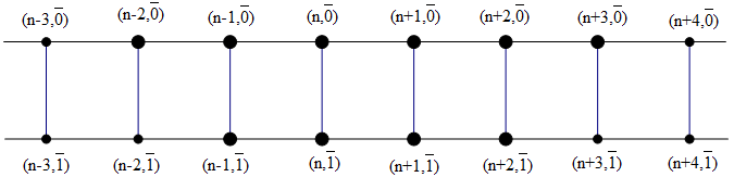
Let $G_{1}$ be a nilpotent group with finite symmetric generating subset $S_{1}$ and $deg(G_{1})=d$ . Let $G_{2}$ be the infinite dihedral group and $S_{2}=\left\{r,s\right\}$ . Set $G=G_{1}\times G_{2}$ . Then

{\rm mdim}_{H}(\mathcal{X},\left\{B_{S_{1}}(n)\right\},d)={\rm mdim}_{M}(\mathcal{X},{G_{1}},d)=2\cdot h_{top}(\mathcal{X},{G}).

Similarly, the above examples hold for Theorem 2.2.

Acknowledgements. The first author was supported by the Postgraduate Research Innovation Program of Jiangsu Province (KYCX201162). The first and second author were supported by NNSF of China (11671208 and 11431012). The third author was supported by NNSF of China (11971236,11601235), NSF of Jiangsu Province (BK20161014), NSF of the Jiangsu Higher Education Institutions of China (16KJD110003), China Postdoctoral Science Foundation (2016M591873), and China Postdoctoral Science Special Foundation (2017T100384). The work was also funded by the Priority Academic Program Development of Jiangsu Higher Education Institutions. We would like to express our gratitude to Tianyuan Mathematical Center in Southwest China, Sichuan University and Southwest Jiaotong University for their support and hospitality.

References

[1] R. Adler, A. Konheim and J. McAndrew, Topological entropy, Trans. Amer. Math. Soc. 114 (1965), 309-319.
[2] H. Bass, The degree of polynomial growth of finitely generated nilpotent groups, Pro. London Math. Soc. 25 (1972), 603-614.
[3] E. Chen and J. Xiong, Dimension and measure theoretic entropy of a subshift in symbolic space, Chinese Sci. Bull. 42 (1997), 1193-1196.
[4] E. Chen, D. Dou and D. Zheng, Variational principle for amenable metric mean dimensions, arxiv:1708.02087.
[5] T. Cover and J. Thomas, Elements of information theory, Wiley, New York, 2006.
[6] M. Coornaert, Topological Dimension and Dynamical Systems, Springer, New York, 2015.
[7] T. Ceccherini-Silberstein and M. Coornaert, Cellular automata and groups, Springer-Verlag, Berlin, 2010.
[8] D. Dou and R. Zhang, A note on dimensional entropy for amenable group actions, Topol. Methods Nonlinear Anal. 51 (2018), 599-608.
[9] H. Furstenberg, Disjointness in ergodic theory, minimal sets, and a problem in Diophantine approximation, Math. Systems Theory. 1 (1967), 1-49.
[10] D. Kerr and H. Li, Ergodic theory : independence and dichotomies, Springer, 2017.
[11] T. Kawabata and A. Dembo, The rate distortion dimension of sets and measures, IEEE Trans.Inf. Theory. 40 (1994), 1564-1572.
[12] E. Lindenstrauss, Pointwise theorems for amenable groups, Invent. Math. 146 (2001), 259-295.
[13] E. Lindenstrauss and M. Tsukamoto, Mean dimension and an embedding problem: an example, Israel J. Math. 199 (2014), 573-584.
[14] E. Lindenstrauss and B. Weiss, Mean topological dimension, Israel J. Math. 115 (2000), 1-24.
[15] E. Lindenstrauss and M. Tsukamoto, From rate distortion theory to metric mean dimension: variational principle, IEEE Trans. Inform. Theory. 64 (2018), 3590-3609.
[16] E. Lindenstrauss and M. Tsukamoto, Double variational principle for mean dimension, Geom. Funct. Anal. 29 (2019), 1048-1109.
[17] H. Li and B. Liang, Mean dimension, mean rank and von Neumann-Luck rank, J. Reine Angew. Math. 739 (2018), 207-240.
[18] T. Meyerovitch and M. Tsukamoto, Expansive multiparameter actions and mean dimension, Trans. Amer. Math. Soc. 371 (2019), 7275-7299.
[19] D. Ornsein and B. Weiss, Entropy and isomorphism theorems for actions of amenable groups, J. Anal. Math. 48 (1987) 1-141.
[20] D. Gatzouras and Y. Peres, Invariant measures of full dimension for some expanding maps, Ergod. Th. Dynam. Sys. 17 (1997), 147-167.
[21] M. Gromov, Topological invariants of dynamical systems and spaces of holomorphic maps, I. Math. Phys. Anal. Geom. 2 (1999), 323-415.
[22] Y. Gutman, E. Lindenstrauss and M. Tsukamoto, Mean dimension of $\mathbb{Z}^{k}$ -actions, Geom. Funct. Anal. 26 (2016), 778-817.
[23] Y. Gutman, Y. Qiao and M. Tsukamoto, Application of signal analysis to the embedding problem of $\mathbb{Z}^{k}$ -actions, Geom. Funct. Anal. 29 (2019), 1440-1502.
[24] Y. Gutman and M. Tsukamoto, Embedding minimal dynamical systems into Hilbert cubes, Invent. math. 221 (2020), 113-166.
[25] M. Tsukamoto, Mean dimension of the dynamical system of Brody curves, Invent. Math. 211 (2018), 935-968.
[26] M. Shinoda and M. Tsukamoto, Symbolic dynamical in mean dimension theory, Ergod. Th. Dynam. Sys. DOI: 10.1017/etds.2020.47
[27] S. Simpson, Symbolic dynamics : Entropy=Dimension=Complexity, Theory Comput. Syst. 56 (2015), 527-543.

	$\displaystyle\dfrac{1}{c_{2}}(s-\epsilon)\|F_{i,j}\|$	$\displaystyle\geq\dfrac{1}{c_{2}}(s-\epsilon)\|B_{S_{1}}((N_{i})\|\|B_{S_{2}}(r_{j}^{i}-1)\|$
		$\displaystyle>(s-\epsilon)\|B_{S_{1}}((N_{i})\|\left(\frac{(r_{j}^{i}-1)(c_{2}-\epsilon)}{c_{2}}\right)$
		$\displaystyle>(s-(h+1)\epsilon)\|B_{S_{1}}(N_{i})\|(r_{j}^{i}-1)$
		$\displaystyle>(s-(h+2)\epsilon)\|B_{S_{1}}(N_{i})\|r_{j}^{i}.~{}~{}(\text{by}~{}\ref{cd})$

	$\displaystyle\|\pi_{B_{S}(N)}(\mathcal{X})\|\cdot 2^{-\frac{1}{c_{2}}(s-\epsilon)(1+\epsilon^{2})\|B_{S}(N)\|}$	$\displaystyle=\sum\limits_{E~{}\text{with}~{}\mathcal{X}_{E}\neq\emptyset}\|\pi_{B_{S}(N)}(\mathcal{X}_{E})\|\cdot 2^{-\frac{1}{c_{2}}(s-\epsilon)(1+\epsilon^{2})\|B_{S}(N)\|}$
		$\displaystyle<2^{(\epsilon^{3}/4c_{2})\|B_{S}(N)\|}\times 2^{(\epsilon^{3}/4c_{2})\|B_{S}(N)\|}$
		$\displaystyle=2^{(\epsilon^{3}/2c_{2})\|B_{S}(N)\|}.$

	$\displaystyle H(X\|Y,Z)$	$\displaystyle\leq\sum\limits_{E\subset B_{S_{1}}(N)}\|E\|\mathbb{P}(Z=E)\log\|B\|$
		$\displaystyle=\mathbb{E}\|Z\|\cdot\log\|B\|$
		$\displaystyle\leq\delta\|B_{S_{1}}(N)\|\log\|B\|.$

Mean dimension theory in symbolic dynamics for finitely generated amenable groups 00footnotetext: * Corresponding author 00footnotetext: 2010 Mathematics Subject Classification: 37B40, 37C85.

1 Introduction

2 Preliminaries

2.1 Finitely generated amenable groups

Remark 2.1.

Definition 2.1.

2.2 Metric mean dimension and mean Hausdorff dimension

Proposition 2.1.

Proof.

2.3 Statement of the main results

Theorem 2.1.

Theorem 2.2.

Remark 2.2.

3 Proof of Theorem 2.1

Proof.

Lemma 3.1.

Proof.

Claim 1.

Proof.

Claim 2.

Proof.

4 Proof of Theorem 2.2

4.1 Mutual information

Lemma 4.1 (Date-Processing inequality).

4.2 Rate distortion theory

4.3 Proof of Theorem 2.2

Proof.

Lemma 4.2.

Proof.

Proof.

5 Examples

Example 5.1.

Example 5.2.

Example 5.3.

References

Mean dimension theory in symbolic dynamics for finitely generated amenable groups ⁰⁰footnotetext: * Corresponding author ⁰⁰footnotetext: 2010 Mathematics Subject Classification: 37B40, 37C85.