Mean-Field Approximation to Gaussian-Softmax Integral with Application to Uncertainty Estimation
Abstract
Many methods have been proposed to quantify the predictive uncertainty associated with the outputs of deep neural networks. Among them, ensemble methods often lead to state-of-the-art results, though they require modifications to the training procedures and are computationally costly for both training and inference. In this paper, we propose a new single-model based approach. The main idea is inspired by the observation that we can “simulate” an ensemble of models by drawing from a Gaussian distribution, with a form similar to those from the asymptotic normality theory, infinitesimal Jackknife, Laplacian approximation to Bayesian neural networks, and trajectories in stochastic gradient descents. However, instead of using each model in the “ensemble” to predict and then aggregating their predictions, we integrate the Gaussian distribution and the softmax outputs of the neural networks. We use a mean-field approximation formula to compute this analytically intractable integral. The proposed approach has several appealing properties: it functions as an ensemble without requiring multiple models, and it enables closed-form approximate inference using only the first and second moments of the Gaussian. Empirically, the proposed approach performs competitively when compared to state-of-the-art methods, including deep ensembles, temperature scaling, dropout and Bayesian NNs, on standard uncertainty estimation tasks. It also outperforms many methods on out-of-distribution detection.
Keywords: Uncertainty Estimation
1 Introduction
Deep neural nets are known to output overconfident predictions. For critical applications such as autonomous driving and medical diagnosis, it is thus necessary to quantify accurately the uncertainty around those predictive outputs. As such, there has been a fast-growing interest in developing new methods for uncertainty estimation.
In this paper, we consider feedforward neural nets for supervised learning of multi-way classifiers. We provide more discussions of (predictive) uncertainty estimation methods in §5 and cite a few here. They fall into three categories: a single pass of a trained model to output both a categorical prediction and the associated probabilities (Guo et al., 2017), multiple passes of an ensemble of different models so that the outputs are aggregated (Lakshminarayanan et al., 2017), and Bayesian approaches that output predictive posterior distributions (MacKay, 1992). The single-pass methods demand low on computation and memory. The ensemble approaches need to train a few models, and also need to keep them around during test time, thus incurring higher computational costs and memory requirement. Bayesian neural networks are principled at incorporating prior knowledge though they are non-trivial to implement and the intractable posterior inference is often a serious challenge. (Conceptually, we can also view Bayesian neural networks as an ensemble of an infinite number of models drawn from the posterior distribution.) While how to evaluate those techniques is an important research topic and has its own cautionary tales, on many popular benchmark datasets, some of the ensemble approaches have consistently attained state-of-the-art performances (Ashukha et al., 2020).
We study how we can achieve the competitive performance of ensemble methods while reducing their demand on computation and memory. Arguably, the competitive performance stems from aggregating (diverse) models. Our main idea is thus inspired by the thought that we can pretend having an ensemble where the models are drawn from a multivariate Gaussian distribution. The mean and the covariance matrix of the distribution describe the models succinctly. However, for neural networks used for classification, integrating this distribution with their softmax output layers, so as to aggregate the models’ outputs, is analytically intractable, as Bayesian posterior inference has encountered.
We make two contributions. The first is to introduce a simple but effective approximation trick called mean-field Gaussian-Softmax (Daunizeau, 2017) and extend it with several variations for uncertainty estimation. The method generalizes the Gaussian-sigmoid integral, a well-known approximation frequently used in machine learning (Bishop, 2006). Likewise, it needs only the first and the second moments of Gaussian random variables and uses them in calculating the probabilistic outputs. The resulting approximation scheme is also intuitive. In its simplest form, it provides an adaptive, data-dependent temperature scaling to the logits, analogous to the well-known approach of global temperature scaling (Guo et al., 2017).
Secondly, the specific form (Eq. (17)) of the Gaussian distribution we assume for the pretended ensemble is also very well connected to many ideas in the literature. Its form is the same as asymptotic normal distribution of parameters111We emphasis that this is just similar in superficial appearance. The theory does not apply in its full generality since neural networks are not identifiable.. It can be motivated from the infinitessimal jackknife technique (Schulam and Saria, 2019; Giordano et al., 2018, 2019; Koh and Liang, 2017), where regularity conditions for asymptotic normality are relaxed. It can also be seen as the Laplace approximation of Bayesian neural networks (MacKay, 1992; Izmailov et al., 2018; Mandt et al., 2017); or the sampling distribution of models collected on training trajectories (Chen et al., 2016; Maddox et al., 2019). Yet, despite the frequent appearance, to the best of our knowledge, none of those prior works has developed the proposed approximate inference approach for uncertainty quantification. In particular, the typical strategy resorts to sampling from the Gaussian distribution and performing Monte Carlo approximation to the integral, a computation burden we explicitly want to reduce.
We show combining these two lead to a method (mfGS) that often surpasses or is as competitive as existing approaches in uncertainty quantification metrics and out-of-distribution detection on all benchmark datasets. It has several appealing properties: constructing the Gaussian distribution does not add significant burden to existing training procedures; approximating the ensemble with a distribution removes the need of storing many models – an impractical task for modern learning models. Due to its connection to Bayesian neural networks, existing approaches in computational statistics such as Kronecker product factorization can be directly applied to accelerate computation and improve scalability.
2 Problem Setup
We are interested in developing a simple and effective way to compute approximately
| (1) |
where the is used to transform to a -dimensional probabilistic output of a deep neural network parameterized with . This integral is a recurring theme in Bayesian learning where the density is the posterior distribution (Bishop, 2006). The posterior distribution is interpreted as epistemic uncertainty and the resulting is treated as the predictive uncertainty. This form also encompasses many ensemble methods where is a discrete measure, representing each model (see below). The integral is not analytically tractable, even for “simple” distributions such as Gaussian. As such, one often resorts to Monte Carlo sampling to approximate it. We seek to avoid that.
In the following, we introduce the notations and provide more detailed contexts that motivate this problem.
Notation
We focus on (deep) feedforward neural network for -way classification. We are given a training set of i.i.d. samples , where with the input and the target . The output of the neural network is denoted by .
We optimize the model’s parameter
| (2) |
where the loss is given by the sum of per-sample loss . In this work, we primarily focus on being the negative -likelihood, though other losses can also be considered (§4.3). The subscript signifies the number of training points – a convention in mathematical statistics. See §4.3 for more examples.
We are interested in not only the categorical prediction on ’s class but also the uncertainty of making such a prediction. We want the softmax probability to accurately represent the probability of belonging to the -th class,
| (3) |
where the activation (or logits) is a linear transformation of the last-layer features , with the -th column of the last layer parameter (matrix) :
| (4) |
In this notation, the neural network parameter is the union of for all bottom layers and in the last layer.
Ensemble Methods
A classic yet very effective idea to improve the estimation Eq. (3) is to use an ensemble of models. Let denote the collection of models. The aggregated predictions is then
| (5) |
where the predictions (and activations) are computed using each model’s parameters. However, obtaining and storing copies of parameters is a serious challenge in both computation and memory, especially for large models. Besides, during inference it is necessary to do passes of different models to compute .
Eq. (5) can be seen as the Monte Carlo approximation to Eq. (1), if we treat as a sample drawn from a distribution of models . Now at least we do not have to keep the models around as the distribution implicitly “memorizes” the models. In this perspective, the ensemble approach is clearly related to Bayesian neural networks (BNN) when is the posterior distribution and the loss function is based on a likelihood function and a prior on the model parameters.
However, there are still two issues to be resolved for the above conceptual framing to be practical. First, how do we choose ? Naturally we want to avoid as much as possible the cost of training multiple times and fit a distribution to the models. Ideally, we want to train one model and use it to derive the distribution.
Secondly, how do we make Eq. (1) computationally tractable for the chosen ? Due to the nonlinearity of the softmax, unless is a distribution or a discrete measure (i.e., the ensemble), the integral is not analytically tractable. Even if we have a way to sample from , resorting to sampling to compute the integral, as commonly used in Bayesian inference, will still make us face the same challenge of multiple passes of models as in Eq. (5).
3 Gaussian-Softmax Integral
Consider the following integral with respect to a -dimensional Gaussian variable ,
| (6) |
Eq. (29) aggregates many classifiers’s softmax outputs where is each model’s logits. This integral is not analytically tractable. We introduce a mean-field approximation scheme to compute it, without resorting to Monte Carlo sampling.
3.1 Mean-Field Approximation
The main steps of the approximation scheme Eq.(11) in this subsection also appeared in (Daunizeau, 2017), though the author there did not use it or other forms Eq.(9,10) for uncertainty estimation. Addiditionally, we discuss the intuitions of those approximations (§3.2), extend them with two temperatures for additional control (§4), and showed that the simpler form of Eq.(9) is equally successful (§6).
The case is well-known (Bishop, 2006, p. 219)
| (7) |
where the softmax becomes the sigmoid function . is a constant and is usually chosen to be or . To generalize to , we rewrite the integral Eq. (29) so that we compare to with , drawing close to Eq. (7),
| (8) |
where “mean field” (MF) “pushes” the integral through each sigmoid term independently222This approximation is prompted by the MF approximation for nonlinear functions . Moreover, we have factorized the to be integrated as “pairwise factors”, i.e. , and apply to them – this is the structural mean-field approach by factorizing joint distributions into “smaller” factors (Koller and Friedman, 2009).. Next we plug in the approximation Eq. (7) to compute the inside expectations.
Mean-Field 0 (mf0)
We ignore the variance of for and replace with its mean , and compute the expectation only with respect to . We arrive at
| (9) |
Mean-Field 1 (mf1)
If we replace with the two independent marginals in the denominator, recognizing , we get,
| (10) |
Mean-Field 2 (mf2)
Lastly, if we compute Eq.(8) with a full covariance between and , recognizing , we get
| (11) |
3.2 Intuition and Remarks
Any of the 3 forms has approximation errors that depend on how “nonlinear” the integrand is. If one class is dominant over others, the softmax is similar to the sigmoid, where the approximation is well-known and applied in practice. We leave more precise quantification of those errors to future studies and focus in this work on their empirical utility. In particular, the simple forms of mfGS make it possible to understand them intuitively.
First, note that when , i.e., reduces to a distribution, mfGS approximations become exact
| (12) |
Namely, if there is no uncertainty associated with , the model should output the regular softmax — this is a desirable sanity check of the approximation schemes. However, when has variance, each scheme handles it differently.
mf0 is especially interesting. The is similar to the regular softmax with a temperature
| (13) |
However, as opposed to the regular temperature scaling factor (Guo et al., 2017), is adaptive as it depends on the variance of a particular sample to be predicted. If the activation on the -th class has high variance, the temperature for that category is high, reducing the corresponding “probability” . Specifically,
| (14) |
In other words, the scaling factor is category and input-dependent, providing additional flexibility to a global temperature scaling factor.
mf1 and mf2 differ from mf0 in how much information from is considered: the variance or additionally the covariance . The effect is to measure how much the -th class should be confused with the -th class after taking into consideration the variances in those classes. Note that mf0 and mf1 are computationally preferred over mf2 which uses covariances, where is the number of classes.
Renormalization Note that if Eq. (29) is computed exactly, all should sum to 1. However, due to the category-specific scaling in the approximation schemes, is no longer a properly normalized probability. Thus we renormalize as,
| (15) |
and similarly for mf1 and mf2 too.
4 Uncertainty Estimation
In this section, we describe how to apply mfGS to the uncertainty estimation problem described in §2.
4.1 The Form of
We propose to use a Gaussian for in Eq. (1):
| (16) |
where is the neural network parameter of the solution (Eq. (2)). is a global ensemble temperature controlling the spread of the Gaussian by scaling the covariance matrix. The covariance is
| (17) |
where the Hessian and the variance of the gradients are defined as follows, computed at ,
| (18) |
The Gaussian is used not only because it is convenient but also the forms of have been occurring frequently in the literature as ways to capture the variations in estimations of model parameters. In §4.3, we will discuss the theoretical rationales behind the choices, after we describe how to use them for uncertainty estimation. (As a preview to our results, performs the best empirically.)
4.2 Mean-field for Uncertainty Estimation
To compute Eq. (1), we make one final approximation, borrowing the linear perturbation idea from the influence function (Cook and Weisberg, 1982), or infinitessimal jackknife, see Eq. (27) in §4.3. Consider the logits (Eq. (4)) when is close to ,
| (19) |
where is the gradient w.r.t. . Under , we have as a Gaussian as well,
| (20) |
Applying any form of mfGS in §3 of computing Gaussian-softmax integral Eq. (29), we obtain a mean-field approximation to Eq. (1). Note that the approximation in Eq. (19) is exact if is a linear function of the parameter, for instance, in the last-layer setting where all layers but the last are treated as being deterministic.
Extension to “Hard”-max
While it is common to think of softmax as outputting soft probabilities, it is also beneficial to introduce a global temperature scaling factor so that we can adjust the “softness” for all the models in the ensemble. Specifically, we use .
Note that and control variability differently. When , each model in the ensemble moves to “hard” decisions. The ensemble average in Eq. (1) thus approaches the majority voting. When , the ensemble focuses on one model, cf. (Wenzel et al., 2020). Empirically, we tune the temperatures and as hyper-parameters on a heldout set, to optimize the predictive performance.
Implementation Algorithm 1 illustrates the main steps of mfGS to estimate uncertainty. Up to two passes through a trained network are needed. If we treat every layer but the last one as a deterministic mapping , we can eliminate the backward pass as the gradient of with respect to the last layer parameter is precisely , already computed in the forward pass. As the empirical study in §6 shows, this setting already leads to very competitive or even the strongest performances.
For smaller models or the aforementioned last-layer setting, computing and storing or is advisable. For very large models, there are well-experimented tricks to approximate; we have used the Kronecker factorization satisfactorily and we only need to formulate those matrices for parameters in each layer independently (Ritter et al., 2018). Others are possible (Pearlmutter, 1994; Agarwal et al., 2016; Koh and Liang, 2017). Note that the computation cost for those matrices are one-time and are amortized.
4.3 Why Using the Gaussians in Eq. (17)?
Readers who are familiar with classical results in theoretical statistics and Bayesian statistics can easily identify the origins of the forms in Eq. (17). An accessible introduction is provided in (Geyer, 2013). Despite being widely known, they have not been applied extensively to deep learning uncertainty estimation. We summarize them briefly as follows.
In the asymptotic normality theory of maximum likelihood estimation, for identifiable models, if the model is correctly specified and the true parameter is , the maximum likelihood estimation converges in distribution to a Gaussian
| (21) |
where is the Fisher information matrix, and equals to the variance of the gradients 333The notation is used in (Geyer, 2013). The subscript 1 refers to sample size 1. and .. In practice, the observed Fisher is often used, and only requires the first-order derivatives:
| (22) |
If the model is misspecified, the estimator converges to the so-called “sandwich” estimator
| (23) |
The true model parameter is unknown and so we use a plug-in estimation such as , resulting Eq. (16).
Neural networks are not identifiable so the asymptotic normality theory does not apply. However, the following infinitessimal jackknife technique can also be used to motivate the use of those Gaussians. Jackknife is a well-known resampling method to estimate the confidence interval of an estimator (Tukey, 1958; Efron and Stein, 1981). Each element is left out from the dataset to form a unique “leave-one-out” Jackknife sample , giving rise to
| (24) |
We obtain an ensemble of such samples and use them to estimate the variances of and the predictions made from . However, it is not feasible to retrain modern neural networks times. Infinitesimal jackknife approximates the retraining (Jaeckel, 1972; Koh and Liang, 2017; Giordano et al., 2018). The basic idea is to approximate with a small perturbation to , i.e., infinitessimal jackknife
| (25) |
where is the Hessian Eq. (18). We fit the copies of with a Gaussian distribution
| (26) |
which is very similar to the asymptotic normality results. The perturbation idea can also be used to approximate any differentiable function , e.g. the logits in Eq. (19).
| (27) |
If we extend the above procedure and analysis to bootstrapping (i.e., sampling with replacement), we will arrive at the following Gaussian to characterize infinitessimal bootstraps:
| (28) |
More details can be found in (Giordano et al., 2018). Finally, the Laplace approximation in Bayesian neural networks uses to approximate the posterior distribution where is the maximum-a-posterior estimate.
In short, all those Gaussian approximations to the true distribution of (i.e. the epistemic uncertainty) share the similar form as Eq. (17) with an added temperature controlling the scaling factor (such as ).
5 Related Work
Ensemble methods have a long history in statistics and machine learning. Despite their effectiveness and often superior performance in uncertainty quantification, it is challenging to apply them to deep learning as they require training multiple copies of models and keeping the models in the memory during testing time.
Obtaining a diverse set of models to aggregate is important. This involves changing training strategy: random initialization and hyperparameters (Lakshminarayanan et al., 2017; Ashukha et al., 2020), using different data partitions such as resampling or bootstraps (Schulam and Saria, 2019; Efron, 1992), collecting models on training trajectories (Chen et al., 2014, 2016; Maddox et al., 2019; Huang et al., 2017). For Bayesian neural networks (BNN) as an ensemble of an infinite number of models, it is important also for sampling or variational inference to aggregate predictions from models drawn from the posterior distributions (Barber and Bishop, 1998; Gal and Ghahramani, 2016; Blundell et al., 2015; Ritter et al., 2018; MacKay, 1992; Wenzel et al., 2020).
Our work is inspired by two observations. Classical results from theoretical statistics describe the convergence of a series of models asymptotically to normal distributions (Geyer, 2013; Giordano et al., 2018, 2019). Yet, using such models as an ensemble, or equivalently, the distribution, for uncertainty estimation is under-explored. Secondly, real-world applications would require us to compute the Gaussian-Softmax integral approximately without resorting to sampling to lower the computational cost. While approximating for Gaussian-sigmoid integral is a well-known result for Bayesian logistic regression, extending it to softmax is less common. Our empirical studies suggest its outstanding utility in matching or exceeding state-of-the-art methods.
Last but not least, recent work in evidential deep learning or prior networks treat the outputs of neural nets as samples of a Dirichlet distribution (Sensoy et al., 2018; Malinin and Gales, 2018; Hobbhahn et al., 2020). They are also single-pass methods and have shown promising results and we compare to one of them in the empirical studies.
6 Experiments
We first describe the setup. We then analyze the effectiveness of the mfGS approximation schemes. We then provide a detailed comparison to state-of-the-art and other popular approaches for uncertainty estimation.
6.1 Setup
We provide key information in the following. For more details, please see the Suppl. Material.
Evaluation Tasks and Metrics We evaluate on two tasks: predictive uncertainty on in-domain samples, and detection of out-of-distribution samples. For in-domain predictive uncertainty, we report classification error rate (), negative log-likelihood (NLL), and expected calibration error in distance (ECE ) on the test set (Guo et al., 2017).
NLL measures the KL-divergence between the empirical label distribution and the predictive distribution of the classifiers. ECE measures the discrepancy between the histogram of the predicted probabilities by the classifiers and the observed ones in the data – properly calibrated classifiers should yield matching histograms. Both metrics are commonly used in the literature and the lower the better.
On the task of out-of-distribution (OOD) detection, we assess how well , the classifier’s output being interpreted as probability, can be used to distinguish invalid samples from normal in-domain ones. Following the common practice (Hendrycks and Gimpel, 2016; Liang et al., 2017; Lee et al., 2018), we report two threshold-independent metrics: area under the receiver operating characteristic curve (AUROC), and area under the precision-recall curve (AUPR). Since the precision-recall curve is sensitive to the choice of positive class, we report both “AUPR in:out” where in-distribution and out-of-distribution samples are swapped. We also report detection accuracy, the optimal accuracy achieved among all thresholds in classifying in-/out-domain samples. All three metrics are the higher the better.
Datasets For in-domain tasks, we use 4 image datasets: MNIST, CIFAR-10, CIFAR-100, and ImageNet (ILSVRC-2012) (LeCun et al., 1998; Krizhevsky, 2009; Deng et al., 2009). For out-of-domain detection, another 4 datasets are used: NotMNIST, LSUN (resized), SVHN and ImageNet-O (Bulatov, 2011; Yu et al., 2015; Netzer et al., 2011; Hendrycks et al., 2019). In the Suppl. Material, we list their descriptive statistics. In short, all but ImageNet have about 50K images for training, 1K to 5K for validation and about 10K images for testing, in 10 to 100 classes. ImageNet is significantly larger: about 1.2 million, 25K and 25K for training, validation and testing, in 1000 classes.
Classifiers For MNIST, we train a two-layer MLP with 256 ReLU units per layer, using Adam optimizer for 100 epochs. For CIFAR-10, we train a ResNet-20 with Adam for 200 epochs. On CIFAR-100, we train a DenseNet-BC-121 with SGD optimizer for 300 epochs. For ImageNet, we train a ResNet-50 with SGD optimizer for 90 epochs.
Methods to Compare We compare to state-of-the-art and popular approaches: the point estimate of maximum likelihood estimator (MLE), the temperature scaling calibration (T. Scale) (Guo et al., 2017), evidential deep learning (EDL) or prior networks (Sensoy et al., 2018; Malinin and Gales, 2018), the deep ensemble method (Deep E.) (Lakshminarayanan et al., 2017), Jackknife (JKnife) (Efron and Stein, 1981), and the resampling infinitessimal bootstrap RUE (Schulam and Saria, 2019). For variants of Bayesian neural networks (BNN), we compare to Dropout (Gal and Ghahramani, 2016), BNN(VI), BNN(KFAC) (Ritter et al., 2018), and SWAG (Maddox et al., 2019).
Tuning We use the NLL and AUROC on the held-out sets to tune hyper-parameters and for in-domain and out-domain tasks respectively. All methods use the same classifier architecture. We also follow the published guidelines on tuning methods we compare to. For EDL, we use the publicly available code (Sensoy, 2018) and tuned accordingly. We will make public the implementation of our method (best temperatures are in the Suppl. Material).
| MNIST | NotMNIST | |||||
| In-domain ( | OOD detection () | |||||
| NLL | ECE | Acc. | ROC | PR(in : out) | ||
| mfGS with versus Sampling with samples | ||||||
| 1.7 | 0.06 | 0.4 | 87.6 | 93.5 | 91.7 : 94.3 | |
| 1.7 | 0.05 | 0.5 | 90.1 | 95.6 | 94.6 : 96.1 | |
| 1.7 | 0.05 | 0.5 | 90.8 | 96.2 | 95.8 : 96.5 | |
| mf0 | 1.7 | 0.05 | 0.2 | 91.9 | 96.9 | 96.7 : 97.0 |
| mf1 | 1.7 | 0.05 | 0.5 | 91.9 | 96.9 | 96.7 : 97.0 |
| mf2 | 1.7 | 0.05 | 0.5 | 91.9 | 96.9 | 96.7 : 97.0 |
| mean-field mf0 with different covariances | ||||||
| 1.7 | 0.05 | 0.2 | 90.8 | 96.1 | 95.9 : 96.2 | |
| 1.7 | 0.05 | 0.3 | 87.0 | 93.4 | 92.1 : 94.0 | |
| SWAG | 1.6 | 0.05 | 0.3 | 87.6 | 93.3 | 91.5 : 94.0 |
| Layers | MNIST | NotMNIST | ||||
| In-domain ( | OOD detection () | |||||
| NLL | ECE | Acc. | ROC | PR(in:out) | ||
| Sampling with samples with different layers. | ||||||
| last layer | 1.7 | 0.05 | 0.5 | 90.8 | 96.2 | 95.8 : 96.5 |
| top two layers | 1.7 | 0.05 | 0.5 | 90.9 | 96.2 | 96.0 : 96.4 |
| all three layers | 1.7 | 0.06 | 0.4 | 87.5 | 92.5 | 87.0 : 93.5 |
| mf0 with different layers. | ||||||
| last layer | 1.7 | 0.05 | 0.2 | 91.9 | 96.9 | 96.7 : 97.0 |
| top two layers | 1.7 | 0.05 | 0.3 | 91.9 | 96.9 | 96.7 : 97.0 |
| all three layers | 1.7 | 0.05 | 0.3 | 91.9 | 96.9 | 96.8 : 97.0 |
Method CIFAR-100 ImageNet CIFAR-100 versus LSUN ImageNet versus ImageNet-O (%) NLL ECE (%) (%) NLL ECE (%) Acc. ROC PR (in:out) Acc. ROC PR (in:out) Deep E. (5) 19.6 0.71 2.00 21.2 0.83 3.10 74.4 82.3 85.7 : 77.8 60.1 50.6 78.9 : 25.7 T. Scale 24.3 0.92 3.13 23.7 0.92 2.09 76.6 84.3 86.7 : 80.3 58.5 54.5 79.2 : 27.8 BNN(KFAC) 24.1 0.89 3.36 23.6 0.92 2.95 72.9 80.4 83.9 : 75.5 60.3 53.1 79.6 : 26.9 mf0 24.3 0.91 1.49 23.7 0.91 0.93 82.2 89.9 92.0 : 86.6 63.2 62.9 83.5 : 33.3 mf1 24.3 0.91 2.20 23.7 0.91 1.17 82.2 89.9 92.0 : 86.6 63.2 62.9 83.5 : 33.3 mf2 24.3 0.91 2.22 23.7 0.91 1.17 82.2 89.9 92.0 : 86.6 63.2 62.9 83.5 : 33.3
| MNIST | NotMNIST | |||||
| In-domain ( | OOD detection () | |||||
| NLL | ECE | Acc. | ROC | PR(in : out) | ||
| Deep E. (5) | 1.3 | 0.05 | 0.3 | 86.5 | 88.0 | 70.4 : 92.8 |
| Deep E. (500) | 1.2 | 0.04 | 0.2 | 92.9 | 96.1 | 90.6 : 96.6 |
| JKnife (500) | 1.2 | 0.04 | 0.3 | 93.4 | 96.6 | 91.8 : 97.0 |
| RUE | 1.7 | 0.08 | 0.9 | 61.1 | 64.7 | 60.5 : 68.4 |
| MLE | 1.7 | 0.10 | 1.2 | 67.6 | 53.8 | 40.1 : 72.5 |
| T. Scale | 1.7 | 0.06 | 0.7 | 67.4 | 66.7 | 48.8 : 77.0 |
| EDL | 1.8 | 0.09 | 1.1 | 83.1 | 80.9 | 59.8 : 90.1 |
| Dropout | 1.7 | 0.06 | 0.7 | 88.8 | 91.4 | 78.7 : 93.5 |
| BNN(VI) | 1.7 | 0.14 | 1.1 | 86.9 | 81.1 | 59.8 : 89.9 |
| BNN(KFAC) | 1.7 | 0.06 | 0.2 | 88.7 | 93.5 | 89.1 : 93.8 |
| mf0 | 1.7 | 0.05 | 0.2 | 91.9 | 96.9 | 96.7 : 97.0 |
6.2 How Good is Mean-field Approximation?
We validate mfGS by comparing it to Monte Carlo sampling for computing the integral Eq. (29). Since there is no ground-truth to this integral, we validate its utility in estimating predictive uncertainty as a “downstream task”. To this end, we use the MNIST and NotMNIST datasets and perform uncertainty estimation with only the last layer.
In Table 1, results from all mean-field approximation schemes are better than those from sampling, in both in-domain and out-domain metrics. Note that while sampling could be improved by increasing samples (thus, more computational costs and memory demands), the mean-field approaches still manage to outperform, especially on the OOD metrics, probably because sampling requires a significantly more samples to converge (the observed improvement is at a fairly slow rate, preventing us from trying more samples.).
Among the 3 schemes, mf0 performs better in ECE, an in-domain task metric while being identical to others. This might be an interesting observation worthy of further investigation. One possible explanation is that for OOD samples, the variances of the logits are such that , i.e. 444Eq. (20) after proper vectorization and padding. is diagonally dominant – the features of an OOD is in the null space of . This is intuitive as should contain vectors maximizing inner products with features from the in-domain samples.
Among 3 choices of selecting in Eq. (17), has a clear advantage over the other two and , though is reasonably good. We also experimented with the covariance matrix derived from the samples on the training trajectories, i.e. SWAG. SWAG performs similar as mf0 with . This is re-assuring as it confirms the theoretical analysis that SWAG converges to the sandwich estimator when its trajectory is in the vicinity of the MLE (Maddox et al., 2019).
In short, the study suggests the mfGS approximation has high quality, measured in the metrics of the “downstream” task of uncertainty estimation. Thus, in the rest of the paper, we focus on mf0 using as .
6.3 Use More Layers for Uncertainty Estimation
In this section, we study the effect of using different number of layers of parameters in mfGS for uncertainty estimation. We report both sampling and mf0 results in Table 2.
mf0 consistently outperforms Monte Carlo sampling. We also observe that using more layers than the last layer does not further help. This is in line with recent studies (Zeng et al., 2018; Kristiadi et al., 2020) showing that last-layer Bayesian approximation can yield good performances in uncertainty tasks. Thus we focus on mfGS with the last layer for the rest of uncertainty estimation experiments.
6.4 mfGS for Uncertainty Estimation
Detailed Comparison on (Not-)MNIST Table 4 contrasts mf0 to ensemble methods, single-pass methods and BNN methods. The ensembles of 5 or 500 models, either with the randomly initialized training (Deep E.) or with JKnife 555We do leave--out training where . clearly dominate in terms of in-domain metrics, closely followed by mf0 and BNN(KFAC). However, in OOD metrics, mf0 clearly dominates others or is on par with the ensemble of 500 JKnife models. RUE does not perform well. We believe its infinitesimal bootstraps, which samples from training examples does not capture the full variations of model parameters, though it does perform better than MLE. Note that other single-pass methods perform the worst.
Ashukha et al. suggest to assess new uncertainty estimate methods by checking the number of models in Deep E. needed to have a matching performance (Ashukha et al., 2020). In OOD metrics, mf0 is about 500 models in Deep E., representing a significant reduction in computational cost and memory requirement — it took about 30 hours on a TitanX GPU to train Deep E. (500) while mf0 needs only one model and a few seconds of inference time. In in-domain metrics, mf0 needs to be improved in accuracy, which is left as future work.
Results on Large-scale Datasets Table 3 extends the comparison on other benchmark datasets, focusing on a few representative and competitive approaches (as seen from Table 4). mf0 dominates all other approaches in OOD metrics by a visible margin. On in-domain task, mf0 falls behind Deep E. on error rates and slightly on NLLs, but significantly improves on ECE. Due to the compute cost, Deep E. used 5 models, as suggested in the original paper (Lakshminarayanan et al., 2017). Additionally, mf0 performs strongly better than either the single-model or the BNN methods in ECE.
More Results in the Suppl. Material Reported there are a fuller Table 3 from other approaches and the dataset CIFAR-10, as well as the analysis of the temperatures and .
7 Conclusion
We propose using mean-field approximation to Gaussian-Softmax integral for uncertainty estimation. This is enabled by “ensembling” the models from a Gaussian distribution whose mean and covariance are readily derived from a trained single model. The proposed approach is compared to many state-of-the-art methods. We find it perform the strongest on identifying out-of-domain samples and is on par with other approaches on in-domain tasks. The method is appealing for its simplicity and effectiveness.
Acknowledgments
Fei Sha is on leave from University of Southern California. This work is partially supported by NSF Awards IIS-1513966/1632803/1833137, CCF-1139148, DARPA Award#: FA8750-18-2-0117, FA8750-19-1- 0504, DARPA-D3M - Award UCB-00009528, Google Research Awards, gifts from Facebook and Netflix, and ARO# W911NF-12-1-0241 and W911NF-15-1-0484.
A More Experiment Results
A.1 An Extended Table 3 of the Main Text
Table 5 provides an extended version of Table 3 in the main text to include results from more approaches. mf0 outperforms all other approaches in OOD metrics including ensemble methods, single-pass methods, and BNN methods. For in-domain tasks, mf0 performs better than either the single-model or BNN methods in ECE. Ensemble performs the strongest in terms of accuracy and NLL.
Method CIFAR-100 ImageNet CIFAR-100 versus LSUN ImageNet versus ImageNet-O (%) NLL ECE (%) (%) NLL ECE (%) Acc. ROC PR (in:out) Acc. ROC PR (in:out) Deep E. (5) 19.6 0.71 2.00 21.2 0.83 3.10 74.4 82.3 85.7 : 77.8 60.1 50.6 78.9 : 25.7 RUE † 24.3 0.99 8.60 23.6 0.92 2.83 75.2 83.0 86.7 : 77.8 58.4 51.6 78.3 : 26.3 MLE 24.3 1.03 10.4 23.7 0.92 3.03 72.7 80.0 83.5 : 75.2 58.4 51.6 78.4 : 26.3 T. Scale 24.3 0.92 3.13 23.7 0.92 2.09 76.6 84.3 86.7 : 80.3 58.5 54.5 79.2 : 27.8 Dropout 23.7 0.84 3.43 24.9 0.99 1.62 69.8 77.3 81.1 : 72.9 59.5 51.7 79.0 : 26.3 BNN(VI) † 25.6 0.98 8.35 26.5 1.17 4.41 62.5 67.7 71.4 : 63.1 57.8 52.0 75.7 : 26.8 BNN(KFAC) 24.1 0.89 3.36 23.6 0.92 2.95 72.9 80.4 83.9 : 75.5 60.3 53.1 79.6 : 26.9 mf0 24.3 0.91 1.49 23.7 0.91 0.93 82.2 89.9 92.0 : 86.6 63.2 62.9 83.5 : 33.3 mf1 24.3 0.91 2.20 23.7 0.91 1.17 82.2 89.9 92.0 : 86.6 63.2 62.9 83.5 : 33.3 mf2 24.3 0.91 2.22 23.7 0.91 1.17 82.2 89.9 92.0 : 86.6 63.2 62.9 83.5 : 33.3
†: Only the last layer is used due to the high computational cost.
A.2 More Results on CIFAR-10 and CIFAR-100
Tables 6 and 7 supplement the main text with additional experimental results on the CIFAR-10 dataset with both in-domain and out-of-distribution detection tasks, and on the CIFAR-100 with out-of-distribution detection using the SVHN dataset. BNN(LL-VI) refers to BNN with stochastic variational inference applied on the last layer only, following Snoek et al. (2019).
The results support the same observations in the main text: mf0 noticeably outperforms other approaches on out-of-distribution detection, but is not as strong as ensemble method in terms of accuracy and NLL. It does in general outperform all other approaches in those two metrics.
Method CIFAR-10 CIFAR-10 verus LSUN CIFAR-10 verus SVHN (%) NLL ECE (%) Acc. ROC PR (in:out) Acc. ROC PR (in:out) Deep E. (5) 6.66 0.20 1.37 88.0 94.4 95.9 : 92.1 88.7 93.4 92.4 : 94.8 RUE 8.71 0.28 1.87 85.0 91.3 93.8 : 87.8 86.3 90.7 89.5 : 92.6 MLE 8.81 0.30 3.59 85.0 91.3 93.8 : 87.8 86.3 90.7 89.5 : 92.6 T. Scale 8.81 0.26 0.52 89.0 95.3 96.5 : 93.4 88.9 94.0 92.7 : 95.0 Dropout 8.83 0.26 0.58 81.8 88.6 91.7 : 84.3 86.0 91.6 90.1 : 94.0 BNN(VI) 11.09 0.33 1.57 79.9 87.3 90.5 : 83.3 85.7 91.4 89.5 : 93.9 BNN(LL-VI) 8.94 0.33 4.15 84.6 91.0 93.5 : 87.2 87.8 93.3 91.7 : 95.4 BNN(KFAC) 8.75 0.29 3.45 85.0 91.3 93.8 : 87.8 86.3 90.7 89.5 : 92.6 mf0 8.81 0.26 0.56 91.0 96.4 97.4 : 94.8 89.7 94.6 93.3 : 95.3
| Method | CIFAR-100 versus SVHN | ||
| Acc. | ROC | PR (in:out) | |
| Deep E. (5) | 75.99 | 83.48 | 77.75 : 88.85 |
| RUE † | 73.90 | 80.69 | 74.03 : 86.93 |
| MLE | 73.90 | 80.69 | 74.03 : 86.93 |
| T. Scale | 76.94 | 83.43 | 77.53 : 88.11 |
| Dropout | 74.13 | 81.87 | 75.78 : 88.07 |
| BNN(VI) † | 71.87 | 79.55 | 72.08 : 87.27 |
| BNN(KFAC) | 74.13 | 80.97 | 74.46 : 87.06 |
| mf0 | 81.38 | 88.04 | 84.59 : 91.23 |
†: Only the last layer is used due to the high computational cost.
A.3 The Effects of and
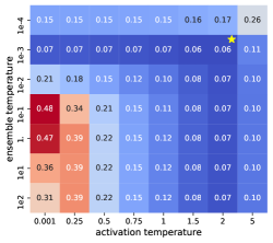
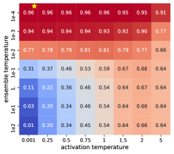
We study the roles of ensemble and activation temperatures in mfGS. controls the how wide we want our Gaussian is and thus determines how many models we would want to integrate. On the other hand, controls how much we want each model in the ensemble to be confident about their predictions.
To this end, on MNIST and NotMNITST datasets we grid search the two temperatures and generate the heatmaps of NLL and AU ROC on the held-out sets, shown in Figure 1. Note that correspond to MLE. What is particularly interesting is that for NLL, higher activation temperature () and lower ensemble temperature () work the best. For area under ROC, however, lower temperatures on both work best. Using for better calibration was also observed in (Guo et al., 2017). On the other end, for OOD detection, (Liang et al., 2017) suggests a very high activation temperature ( in their work, likely due to using a single model instead of an ensemble).
Examining both plots horizontally, we can see when the is higher, the effect of is more pronounced than when is lower. Vertically, we can see when the is lower, the effect of is more pronounced than when is higher, especially on the OOD tasks.
A.4 Robustness to Distributional Shift.
B Unscented Kalman Filter for Gaussian-Softmax Integral
Unscented Kalman Filter (ukf) is a standard numerical technique (Wan and Van Der Merwe, 2000) used in nonlinear estimations to approximate Gaussian integrals. Here we briefly summarize the main steps in ukf.
| Method | MNIST | NotMNIST | ||||
| In-domain ( | OOD detection () | |||||
| NLL | ECE | Acc. | ROC | PR(in:out) | ||
| mf0 | 1.67 | 0.05 | 0.20 | 91.93 | 96.91 | 96.67 : 96.99 |
| ukf | 1.67 | 0.05 | 0.42 | 89.07 | 96.37 | 95.32 : 97.42 |
Assume the Gaussian random variable is of dimensional. ukf approximates the Gaussian-Softmax integral (reiterate Eq.(6) in the main text) by a carefully designed weighted sum on sample points, referred to as sigma points . The sigma points are chosen such that they capture the posterior mean and covariance accurately to the 3rd order Taylor series expansion for any nonlinearity.
| (29) |
The specific form of and are as follows,
| (30) | ||||
| (31) | ||||
| (32) |
where is the -th column of , which is the square root of the covariance matrix . We use the Cholesky factor as and the constant in our implementation.
We plug in ukf approximation and evaluate its performance on uncertainty estimation. We compare ukf with mf0 on MNIST and NotMNIST datasets in Table 8. We also tuned activation and ensemble temperatures for ukf. ukf performs competitively on OOD detection task, but not as well on in-domain ECE compared with mf0.
C Experiment Details
In this section, we provide experimental details for reproducibility.
C.1 Datasets
The statistics of the benchmark datasets used in our experiment are summarized in Table 9.
| Dataset | # of classes | train/held-out/test |
| MNIST | 10 | 55k/5k/10k |
| CIFAR-10 | 10 | 45k/5k/10k |
| CIFAR-100 | 100 | 45k/5k/10k |
| ILSVRC-2012 | 1,000 | 1,281k/25k/25k |
| NotMNIST | - | -/5k/13.7k |
| LSUN (resized) | - | -/1k/9k |
| SVHN | - | -/5k/21k |
| Imagenet-O | - | -/2k/- |
C.2 Definitions of Evaluation Metrics
NLL is defined as the KL-divergence between the data distribution and the model’s predictive distribution,
| (33) |
where is the one-hot embedding of the label.
ECE measures the discrepancy between the predicted probabilities and the empirical accuracy of a classifier in terms of distance. It is computed as the expected difference between per bucket confidence and per bucket accuracy. All predictions are binned into buckets such that are predictions falling within the interval . ECE is defined as,
| (34) |
where and .
C.3 Hyper-parameter Tuning
Hyper-parameters in training Table 10 provides key hyper-parameters used in training deep neural networks on different datasets.
| Dataset | MNIST | CIFAR-10 | CIFAR-100 | ImageNet |
| Architecture | MLP | ResNet20 | Densenet-BC-121 | ResNet50 |
| Optimizer | Adam | Adam | SGD | SGD |
| Learning rate | 0.001 | 0.001 | 0.1 | 0.1 |
| Learning rate decay | exponential | staircase | staircase | staircase |
| 0.998 | at 80, 120, 160 | at 150, 225 | at 30, 60, 80 | |
| Weight decay | 0 | |||
| Batch size | 100 | 8 | 128 | 256 |
| Epochs | 100 | 200 | 30 | 90 |
Hyper-parameters in uncertainty estimation For mf0 method, we use in our implementation. For the Deep E. approach, we use models on all datasets as in (Snoek et al., 2019). For RUE, Dropout, BNN(VI) and BNN(KFAC), where sampling is applied at inference time, we use Monte-Carlo samples on MNIST, and on CIFAR-10, CIFAR-100 and ImageNet. We use buckets when computing ECE on MNIST, CIFAR-10 and CIFAR-100, and on ImageNet.
For in-domain uncertainty estimation, we use the NLL on the held-out sets to tune hyper-parameters. For the OOD detection task, we use area under ROC curve on the held-out to select hyper-parameters. We report the results of the best hyper-parameters on the test sets. The key hyper-parameters we tune are the temperatures, regularization or prior in BNN methods, and dropout rates in Dropout.
Other implementation details When Hessian needs to be inverted, we add a dampening term following (Ritter et al., 2018; Schulam and Saria, 2019) to ensure positive semi-definiteness and the smallest eigenvalue of be 1. For BNN(VI), we use Flipout (Wen et al., 2018) to reduce gradient variances and follow (Snoek et al., 2019) for variational inference on deep ResNets. On ImageNet, we compute the Kronecker-product factorized Hessian matrix, rather than full due to high dimensionality. For BNN(KFAC) and RUE, we use mini-batch approximations on subsets of the training set to scale up on ImageNet, as suggested in (Ritter et al., 2018; Schulam and Saria, 2019).
D Infinitesimal Jackknife and Its Distribution
We include a derivation of infinitesimal jackknife (Eq.(26) in §4.3 of the main text) with more details to be self-contained.
Jackknife is a resampling method to estimate the confidence interval of an estimator (Tukey, 1958; Efron and Stein, 1981). It works as follows: each element is left out from the dataset to form a unique “leave-one-out” jackknife sample . A jackknife sample’s estimate of is given by
| (35) |
We obtain such samples and use them to estimate the variances of and the predictions made with . In this vein, this is a form of ensemble method.
However, it is not feasible to retrain modern neural networks times, when is often in the order of millions. Infinitesimal jackknife is a classical tool to approximate without re-training on . It is often used as a theoretical tool for asymptotic analysis (Jaeckel, 1972), and is closely related to influence functions in robust statistics (Cook and Weisberg, 1982). Recent studies have brought (renewed) interests in applying this methodology to machine learning problems (Giordano et al., 2018; Koh and Liang, 2017). Here, we briefly summarize the method.
Linear approximation. The basic idea behind infinitesimal jackknife is to treat the and as special cases of an estimator on weighted samples,
| (36) |
Thus the maximum likelihood estimate is when . A jackknife sample’s estimate , on the other end, is when where is an all-zero vector except taking a value of at the -th coordinate.
Using the first-order Taylor expansion of around , we obtain (under the condition of twice-differentiability and the invertibility of the Hessian),
| (37) |
where is the Hessian matrix of evaluated at (recall Eq.(18) in the main text), and is the gradient of evaluated at .
An infinite number of infinitesimal jackknife samples. If the number of samples , we can characterize the “infinite” number of with a closed-form Gaussian distribution with the following sample mean and covariance as the distribution’s mean and covariance,
| (38) |
and
| (39) |
where is the observed Fisher information matrix (recall Eq.(18) in the main text).
An infinite number of infinitesimal bootstrap samples. The above procedure and analysis can be extended to bootstrapping (i.e., sampling with replacement). The perturbed estimates from bootstrap samples have
| (40) |
Similarly, to characterize the estimates from the bootstraps, we can also use a Gaussian distribution,
| (41) |
Lakshminarayanan et al. (2017) discussed that using models trained on bootstrapped samples does not work empirically as well as other approaches, as the learner only sees of the dataset in each bootstrap sample. We note that this is an empirical limitation rather than a theoretical one. In practice, we can only train a very limited number of models. However, we hypothesize that we can get the benefits of combining an infinite number of models from the closed-form Gaussian distribution without training. Empirical results valid this hypothesis.
References
- Agarwal et al. (2016) Naman Agarwal, Brian Bullins, and Elad Hazan. Second-order stochastic optimization in linear time. stat, 1050:15, 2016.
- Ashukha et al. (2020) Arsenii Ashukha, Alexander Lyzhov, Dmitry Molchanov, and Dmitry Vetrov. Pitfalls of in-domain uncertainty estimation and ensembling in deep learning. arXiv preprint arXiv:2002.06470, 2020.
- Barber and Bishop (1998) David Barber and Christopher M Bishop. Ensemble learning for multi-layer networks. In Advances in neural information processing systems, pages 395–401, 1998.
- Bishop (2006) Christopher M. Bishop. Pattern Recognition and Machine Learning. Springer, 2006.
- Blundell et al. (2015) Charles Blundell, Julien Cornebise, Koray Kavukcuoglu, and Daan Wierstra. Weight uncertainty in neural networks. arXiv preprint arXiv:1505.05424, 2015.
- Bulatov (2011) Yaroslav Bulatov. Notmnist dataset. Google (Books/OCR), Tech. Rep.[Online]. Available: http://yaroslavvb. blogspot. it/2011/09/notmnist-dataset. html, 2, 2011.
- Chen et al. (2014) Tianqi Chen, Emily Fox, and Carlos Guestrin. Stochastic gradient hamiltonian monte carlo. In International conference on machine learning, pages 1683–1691, 2014.
- Chen et al. (2016) Xi Chen, Jason D Lee, Xin T Tong, and Yichen Zhang. Statistical inference for model parameters in stochastic gradient descent. arXiv preprint arXiv:1610.08637, 2016.
- Cook and Weisberg (1982) R Dennis Cook and Sanford Weisberg. Residuals and influence in regression. New York: Chapman and Hall, 1982.
- Daunizeau (2017) Jean Daunizeau. Semi-analytical approximations to statistical moments of sigmoid and softmax mappings of normal variables. arXiv preprint arXiv:1703.00091, 2017.
- Deng et al. (2009) Jia Deng, Wei Dong, Richard Socher, Li-Jia Li, Kai Li, and Li Fei-Fei. Imagenet: A large-scale hierarchical image database. In 2009 IEEE conference on computer vision and pattern recognition, pages 248–255. Ieee, 2009.
- Efron (1992) Bradley Efron. Bootstrap methods: another look at the jackknife. In Breakthroughs in statistics, pages 569–593. Springer, 1992.
- Efron and Stein (1981) Bradley Efron and Charles Stein. The jackknife estimate of variance. The Annals of Statistics, pages 586–596, 1981.
- Gal and Ghahramani (2016) Yarin Gal and Zoubin Ghahramani. Dropout as a bayesian approximation: Representing model uncertainty in deep learning. In international conference on machine learning, pages 1050–1059, 2016.
- Geyer (2013) Charles J. Geyer. 5601 notes: The sandwich estimator, 2013. http://www.stat.umn.edu/geyer/5601/notes/sand.pdf.
- Giordano et al. (2018) Ryan Giordano, Will Stephenson, Runjing Liu, Michael I Jordan, and Tamara Broderick. A swiss army infinitesimal jackknife. arXiv preprint arXiv:1806.00550, 2018.
- Giordano et al. (2019) Ryan Giordano, Michael I Jordan, and Tamara Broderick. A higher-order swiss army infinitesimal jackknife. arXiv preprint arXiv:1907.12116, 2019.
- Guo et al. (2017) Chuan Guo, Geoff Pleiss, Yu Sun, and Kilian Q Weinberger. On calibration of modern neural networks. arXiv preprint arXiv:1706.04599, 2017.
- Hendrycks and Gimpel (2016) Dan Hendrycks and Kevin Gimpel. A baseline for detecting misclassified and out-of-distribution examples in neural networks. arXiv preprint arXiv:1610.02136, 2016.
- Hendrycks et al. (2019) Dan Hendrycks, Kevin Zhao, Steven Basart, Jacob Steinhardt, and Dawn Song. Natural adversarial examples. arXiv preprint arXiv:1907.07174, 2019.
- Hobbhahn et al. (2020) Marius Hobbhahn, Agustinus Kristiadi, and Philipp Hennig. Fast predictive uncertainty for classification with bayesian deep networks, 2020.
- Huang et al. (2017) Gao Huang, Yixuan Li, Geoff Pleiss, Zhuang Liu, John E Hopcroft, and Kilian Q Weinberger. Snapshot ensembles: Train 1, get m for free. arXiv preprint arXiv:1704.00109, 2017.
- Izmailov et al. (2018) Pavel Izmailov, Dmitrii Podoprikhin, Timur Garipov, Dmitry Vetrov, and Andrew Gordon Wilson. Averaging weights leads to wider optima and better generalization. arXiv preprint arXiv:1803.05407, 2018.
- Jaeckel (1972) Louis A Jaeckel. The infinitesimal jackknife. Bell Telephone Laboratories, 1972.
- Koh and Liang (2017) Pang Wei Koh and Percy Liang. Understanding black-box predictions via influence functions. In Proceedings of the 34th International Conference on Machine Learning-Volume 70, pages 1885–1894. JMLR. org, 2017.
- Koller and Friedman (2009) D. Koller and N. Friedman. Probabilistic Graphical Models: Principles and Techniques. MIT Press, 2009.
- Kristiadi et al. (2020) Agustinus Kristiadi, Matthias Hein, and Philipp Hennig. Being bayesian, even just a bit, fixes overconfidence in relu networks. arXiv preprint arXiv:2002.10118, 2020.
- Krizhevsky (2009) A Krizhevsky. Learning multiple layers of features from tiny images. Master’s thesis, University of Tront, 2009.
- Lakshminarayanan et al. (2017) Balaji Lakshminarayanan, Alexander Pritzel, and Charles Blundell. Simple and scalable predictive uncertainty estimation using deep ensembles. In Advances in Neural Information Processing Systems, pages 6405–6416, 2017.
- LeCun et al. (1998) Yann LeCun, Corinna Cortes, and Christopher JC Burges. The mnist database of handwritten digits, 1998. URL http://yann. lecun. com/exdb/mnist, 10:34, 1998.
- Lee et al. (2018) Kimin Lee, Kibok Lee, Honglak Lee, and Jinwoo Shin. A simple unified framework for detecting out-of-distribution samples and adversarial attacks. In Advances in Neural Information Processing Systems, pages 7165–7175, 2018.
- Liang et al. (2017) Shiyu Liang, Yixuan Li, and R Srikant. Enhancing the reliability of out-of-distribution image detection in neural networks. arXiv preprint arXiv:1706.02690, 2017.
- MacKay (1992) David JC MacKay. Bayesian methods for adaptive models. PhD thesis, California Institute of Technology, 1992.
- Maddox et al. (2019) Wesley J Maddox, Pavel Izmailov, Timur Garipov, Dmitry P Vetrov, and Andrew Gordon Wilson. A simple baseline for bayesian uncertainty in deep learning. In Advances in Neural Information Processing Systems, pages 13132–13143, 2019.
- Malinin and Gales (2018) Andrey Malinin and Mark Gales. Predictive uncertainty estimation via prior networks. In S. Bengio, H. Wallach, H. Larochelle, K. Grauman, N. Cesa-Bianchi, and R. Garnett, editors, Advances in Neural Information Processing Systems 31, pages 7047–7058. Curran Associates, Inc., 2018.
- Mandt et al. (2017) Stephan Mandt, Matthew D Hoffman, and David M Blei. Stochastic gradient descent as approximate bayesian inference. The Journal of Machine Learning Research, 18(1):4873–4907, 2017.
- Netzer et al. (2011) Yuval Netzer, Tao Wang, Adam Coates, Alessandro Bissacco, Bo Wu, and Andrew Ng. Reading digits in natural images with unsupervised feature learning. NIPS, 01 2011.
- Pearlmutter (1994) Barak A Pearlmutter. Fast exact multiplication by the hessian. Neural computation, 6(1):147–160, 1994.
- Ritter et al. (2018) Hippolyt Ritter, Aleksandar Botev, and David Barber. A scalable laplace approximation for neural networks. In 6th International Conference on Learning Representations, ICLR 2018-Conference Track Proceedings, volume 6. International Conference on Representation Learning, 2018.
- Schulam and Saria (2019) Peter Schulam and Suchi Saria. Can you trust this prediction? auditing pointwise reliability after learning. arXiv preprint arXiv:1901.00403, 2019.
- Sensoy (2018) Murat Sensoy. Github code: Evidential deep learning to quantify classification uncertainty, 2018. https://muratsensoy.github.io/uncertainty.html.
- Sensoy et al. (2018) Murat Sensoy, Lance Kaplan, and Melih Kandemir. Evidential deep learning to quantify classification uncertainty. In S. Bengio, H. Wallach, H. Larochelle, K. Grauman, N. Cesa-Bianchi, and R. Garnett, editors, Advances in Neural Information Processing Systems 31, pages 3179–3189. Curran Associates, Inc., 2018.
- Snoek et al. (2019) Jasper Snoek, Yaniv Ovadia, Emily Fertig, Balaji Lakshminarayanan, Sebastian Nowozin, D Sculley, Joshua Dillon, Jie Ren, and Zachary Nado. Can you trust your model’s uncertainty? evaluating predictive uncertainty under dataset shift. In Advances in Neural Information Processing Systems, pages 13969–13980, 2019.
- Tukey (1958) John Tukey. Bias and confidence in not quite large samples. Ann. Math. Statist., 29:614, 1958.
- Wan and Van Der Merwe (2000) Eric A Wan and Rudolph Van Der Merwe. The unscented kalman filter for nonlinear estimation. In Proceedings of the IEEE 2000 Adaptive Systems for Signal Processing, Communications, and Control Symposium (Cat. No. 00EX373), pages 153–158. Ieee, 2000.
- Wen et al. (2018) Yeming Wen, Paul Vicol, Jimmy Ba, Dustin Tran, and Roger Grosse. Flipout: Efficient pseudo-independent weight perturbations on mini-batches. arXiv preprint arXiv:1803.04386, 2018.
- Wenzel et al. (2020) Florian Wenzel, Kevin Roth, Bastiaan S Veeling, Jakub Światkowski, Linh Tran, Stephan Mandt, Jasper Snoek, Tim Salimans, Rodolphe Jenatton, and Sebastian Nowozin. How good is the bayes posterior in deep neural networks really? arXiv preprint arXiv:2002.02405, 2020.
- Yu et al. (2015) Fisher Yu, Ari Seff, Yinda Zhang, Shuran Song, Thomas Funkhouser, and Jianxiong Xiao. Lsun: Construction of a large-scale image dataset using deep learning with humans in the loop. arXiv preprint arXiv:1506.03365, 2015.
- Zeng et al. (2018) Jiaming Zeng, Adam Lesnikowski, and Jose M Alvarez. The relevance of bayesian layer positioning to model uncertainty in deep bayesian active learning. arXiv preprint arXiv:1811.12535, 2018.