This paper was converted on www.awesomepapers.org from LaTeX by an anonymous user.
Want to know more? Visit the Converter page.

Mean field limits of particle-based stochastic reaction-drift-diffusion models

M. Heldman1,2 1 Department of Mathematics, Virginia Tech, Blacksburg, VA 24061 2 Department of Mathematics and Statistics, Boston University, Boston, MA 02215 maxh@vt.edu S. A. Isaacson2 isaacsas@bu.edu Q. Liu2 liuq19@bu.edu  and  K. Spiliopoulos2 kspiliop@bu.edu
Abstract.

We consider particle-based stochastic reaction-drift-diffusion models where particles move via diffusion and drift induced by one- and two-body potential interactions. The dynamics of the particles are formulated as measure-valued stochastic processes (MVSPs), which describe the evolution of the singular, stochastic concentration fields of each chemical species. The mean field large population limit of such models is derived and proven, giving coarse-grained deterministic partial integro-differential equations (PIDEs) for the limiting deterministic concentration fields’ dynamics. We generalize previous studies on the mean field limit of models involving only diffusive motion, with care to formulating the MVSP representation to ensure detailed balance of reversible reactions in the presence of potentials. Our work illustrates the more general set of PIDEs that arise in the mean field limit, demonstrating that the limiting macroscopic reactive interaction terms for reversible reactions obtain additional nonlinear concentration-dependent coefficients compared to the purely diffusive case. Numerical studies are presented which illustrate that two-body repulsive potential interactions can have a significant impact on the reaction dynamics, and also demonstrate the empirical numerical convergence of solutions to the PBSRDD model to the derived mean field PIDEs as the population size increases.

S. A. I., M. H., and Q. L. were supported by ARO W911NF-20-1-0244 and National Science Foundation DMS-1902854. K.S. was partially supported by the National Science Foundation DMS-2107856, DMS-2311500, SIMONS Foundation Award 672441 and ARO W911NF-20-1-0244.

1. Introduction

We consider particle-based stochastic reaction-drift-diffusion (PBSRDD) models where particles move via diffusion and drift induced by one- and two-body potential interactions. We formulate the dynamics of the particles as measure-valued stochastic processes (MVSPs), which describe the stochastic evolution of the concentration fields of each chemical species as a sum of δ\delta-functions encoding the position and type of each particle. Our goal is to formulate an appropriate MVSP model for such systems, and then rigorously investigate the large population limit of the MVSP dynamics, deriving partial-integral differential equations (PIDEs) that represent the limiting mean-field dynamics.

Particle-based stochastic reaction-diffusion (PBSRD) models have a long history of use in modeling the diffusion of, and reactions between, individual molecules. PBSRDD models are more macroscopic descriptions than millisecond-timescale quantum mechanical or molecular dynamics models of a few molecules [42], but more microscopic descriptions than deterministic 3D reaction-diffusion PDEs for the average concentration field of each chemical species. One of the most popular PBSRDD models for studying biological processes is the volume reactivity (VR) model of Doi [47, 9, 10]. In the Doi model, the positions of individual molecules are typically represented as points undergoing Brownian motion. Bimolecular reactions between two substrate molecules occur with a probability per unit time based on their current positions [9, 10]. Unimolecular reactions are typically assumed to represent internal processes, and as such are modeled as occurring with exponentially distributed times based on a specified reaction-rate constant.

In our prior work [28], we investigated the large population limit of PBSRD models (i.e. in the absence of drift). Allowing drift makes the models more relevant for applications, but complicates the model formulation and the analysis needed to prove the mean field limit. Many models of biological systems involve drift induced by background potential fields and/or by potential interactions. In modeling cellular processes, the former has been used to model how volume exclusion by DNA fibers impedes protein diffusion in the nucleus [29, 32], and to model membrane-bound protein motion induced by actin contraction in T cell synapses [43]. Two-body potential interaction fields have been used to more accurately account for attractive or repulsive interactions between molecules [23], including to model volume exclusion due to the physical size of molecules [4, 43]. More generally, such interactions can arise in diverse classes of agent-based models including models for the spread of infections or innovations within populations [20], or for interactions between cells. In addition, as our numerical studies in Section 7 demonstrate, the inclusion of potential interactions can have non-trivial effects on the behavior of the system. We therefore now investigate the large population limit PBSRDD models where particles move via diffusion and drift term induced by one-body and two-body potentials.

For simplicity, we will work in free space as in [28, 27], and as such, we will study the large population mean field limit via an increasing scaling parameter, γ\gamma, which can physically represent Avogadro’s number. The “large system size” limit γ\gamma\rightarrow\infty is where one typically obtains more macroscopic coarse-grained partial-integral differential equation (PIDE), PDE, SPIDE, or SPDE models for biological systems that model diffusion and reaction via the evolution of continuous concentration fields [18, 28, 2, 36, 20, 38, 40]. To determine the limit for PBSRDD models we adopt the classical Stroock-Varadhan Martingale approach [12, 46] that previously allowed us to rigorously identify and prove the large population limit of the MVSP representation for PBSRDD models [28]. We note that this method has been successful in many instances to study large population dynamics and general interacting particle systems, see [14, 15, 6, 7, 8, 25, 37, 44]. We identify a new macroscopic system of partial integro-differential equations (PIDEs) whose solution corresponds to the large population limit of the MVSP, and we rigorously prove the convergence (in a weak sense) of the MVSP to this solution.

We also note here that the bottom-up approach that we take in this paper allows us to derive the new macroscopic PIDEs corresponding to the true population limit of the underlying spatial PBSRDD model. This is to be contrasted with the well-known macroscopic reaction-drift-diffusion PDE models of chemical reactions at a cellular scale, which are often derived by modifying standard ODE models for non-spatial reaction systems via the addition of drift-diffusion operators to give a (phenomenological) spatial model. Note, in the absence of potential interactions (i.e., particles move only via diffusion), in [27] we proved that such models can be seen as limits of the rigorous mean field limit we derived in [28] when bimolecular reaction kernels are short-range and averaging.

For our model, consider Γj\Gamma_{j} to be the set of indices of particles of species jj. In the absence of reactions, suppose that the iith particle is of species jj and located at position QtiQ_{t}^{i} at time tt. The iith particle then moves according to

(1) dQti\displaystyle dQ_{t}^{i} =[vj(Qti)+1γj=1,jjJkΓjuj,j(QtiQtk)+1γkΓj,kiuj,j(QtiQtk)]dt\displaystyle=-\biggl{[}\nabla v_{j}(Q_{t}^{i})+\frac{1}{\gamma}\nabla\sum_{j^{\prime}=1,j^{\prime}\neq j}^{J}\sum_{k\in\Gamma_{j^{\prime}}}u_{j,j^{\prime}}\bigl{(}\|Q_{t}^{i}-Q_{t}^{k}\|\bigr{)}+\frac{1}{\gamma}\nabla\sum_{k\in\Gamma_{j},k\neq i}u_{j,j}\bigl{(}\|Q_{t}^{i}-Q_{t}^{k}\|\bigr{)}\biggr{]}dt
+2DjdWti.\displaystyle\qquad+\sqrt{2D^{j}}dW_{t}^{i}.

Here vj(x)v_{j}(x) denotes the one-body potential experienced by a particle of type jj when at position xx, and uj,j(xy)/γu_{j,j^{\prime}}(\|x-y\|)/\gamma the two-body potential between particles at locations xx and yy of types jj and jj^{\prime} respectively. Nζ(t)N^{\zeta}(t) denotes the total number of particles at time tt, and ζ=(1γ,η)\zeta=(\frac{1}{\gamma},\eta) is a vector consisting of the mean field limit scaling parameter, γ\gamma, and a displacement range parameter, η\eta. In the large population mean field limit, γ\gamma plays the role of a system size (e.g., Avogadro’s number, or in bounded domains the product of Avogadro’s number and the domain volume)[1]. η\eta represents a regularization parameter we introduce to rigorously handle δ\delta-function placement densities for reaction products, which are commonly used in many PBSRDD models, see Section 5. Finally, DjD^{j} represents the diffusion coefficient for a particle of species jj, and {Wti}i+\{W_{t}^{i}\}_{i\in\mathbb{N}_{+}} is a countable collection of standard independent Brownian motions in d\mathbb{R}^{d}.

From (1), we see each particle follows the gradient of a potential landscape, the so-called suitability landscape, and also experiences an additional force derived from the two-body potentials. The scaling 1γ\frac{1}{\gamma} in front of the pair-wise potentials is the mean field scaling, which, at least formally, preserves the total strength of the interaction at order one so that we have a well-defined large population mean field limit in the absence of reactions, see [33].

From a mathematical point of view, adding drift due to potential interactions makes the rigorous formulation of the particle model more complicated, and gives rise to a number of new terms that need to be appropriately handled for a coarse-grained mean field limit to exist. Specifically, in moving from PBSRD (purely-diffusive) to PBSRDD models (drift due to potential interactions) reactive interaction functions, which determine the probability per time substrates react and produce products at specified positions, may require modification. Such modifications ensure detailed balance of reaction fluxes, i.e., the statistical mechanical property that the pointwise forward and backward reaction fluxes should balance at equilibrium [31, 13, 17]. When formulating PBSRDD reactive interaction terms to be consistent with detailed balance at equilibrium, the needed modifications result in a dependence on the full potential of the system (hence adding a dependence on the positions of non-reactant particles). We specifically formulate these modifications as an extra rejection/acceptance probability appearing within reactive interaction functions, following the approach proposed in [13], but note our results should be straightforward to adapt should one instead modify reaction rates or product placement mechanisms to ensure detailed balance. One of the contributions of this work is that we make all of these modifications precise in a general fashion via the MVSP formulation. We illustrate our results for a specific, but important, choice of rejection/acceptance probabilities based on the functional choices proposed by Fröhner and Noé [13]. The modified reactive interaction functions we employ then give rise to additional nonlinear concentration-dependent coefficients within the limiting reactive terms of the resulting mean field PIDEs, giving rise to a new deterministic, macroscopic reaction-drift-diffusion model.

To illustrate the main result of this paper, consider the reversible A+BCA+B\rightleftarrows C reaction as an example. Denote the forward A+BCA+B\rightarrow C reaction by 1\mathcal{R}_{1} and the backward CA+BC\rightarrow A+B reaction by 2\mathcal{R}_{2}. Let us represent by A(t)A(t) the stochastic process for the number of species A molecules at time tt, and label the position of iith molecule of species A at time tt by the stochastic process 𝑸iA(t)d\bm{Q}_{i}^{A(t)}\subset\mathcal{R}^{d}. The quantity

Aγ(x,t)=1γi=1A(t)δ(xQiA(t))A^{\gamma}(x,t)=\frac{1}{\gamma}\sum_{i=1}^{A(t)}\delta\bigl{(}x-Q_{i}^{A(t)}\bigr{)}

corresponds to the stochastic, singular molar concentration field of species A at point xx at time tt. We define Bγ(x,t)B^{\gamma}(x,t) and Cγ(x,t)C^{\gamma}(x,t) in a similar fashion, and let 𝐒γ(x,t)=(Aγ(x,t),Bγ(x,t),Cγ(x,t))\mathbf{S}^{\gamma}(x,t)=(A^{\gamma}(x,t),B^{\gamma}(x,t),C^{\gamma}(x,t)). For each species we assume a spatially-constant diffusivity, DA,DBD^{\mathrm{A}},D^{\mathrm{B}} and DCD^{\mathrm{C}}, respectively.

For 1\mathcal{R}_{1}, let K1γ(x,y)K^{\gamma}_{1}(x,y) denote the probability per time that one A molecule at xx and one B\mathrm{B} molecule at yy react. The product CC molecule is then placed at zz following the probability density m1η(z|x,y)m^{\eta}_{1}(z|x,y), conditioning on substrates at xx and yy. Here the displacement range parameter η\eta represents a mollification parameter for singular δ\delta-function placement densities. We further incorporate a rejection/acceptance mechanism via an acceptance probability π1γ(z|x,y,𝒒)\pi^{\gamma}_{1}(z|x,y,\bm{q}), which indicates the probability that the above reaction is accepted, i.e. alllowed to occur, and generates a product at zz given the positions of the substrates at xx and yy, and of the non-substrate and non-product particles molecules at 𝒒\bm{q}. We define K2γ(z),m2η(x,y|z)K_{2}^{\gamma}(z),m^{\eta}_{2}(x,y|z) and π2γ(x,y|z,𝒒)\pi^{\gamma}_{2}(x,y|z,\bm{q}) analogously for the reverse reaction 2\mathcal{R}_{2}. Finally, we assume that the acceptance probabilities can be equivalently rewritten as a function of the substrate positions, product positions, and the pre-reaction concentration fields, π1γ(z|x,y,𝐒γ(x,t)dx)\pi^{\gamma}_{1}\bigl{(}z|x,y,\mathbf{S}^{\gamma}(x^{\prime},t)dx^{\prime}\bigr{)} and π2γ(x,y|z,𝐒γ(x,t)dx)\pi^{\gamma}_{2}\bigl{(}x,y|z,\mathbf{S}^{\gamma}(x^{\prime},t)dx^{\prime}\bigr{)}. In Section 6 we illustrate that this assumption holds for the specific choices of rejection/acceptance probabilities proposed in [13].

Note that K1γ,m1ηK_{1}^{\gamma},m_{1}^{\eta} and π1γ\pi_{1}^{\gamma} all depend on ζ=(1γ,η)\zeta=(\frac{1}{\gamma},\eta). In the large population limit that γ\gamma\rightarrow\infty and η0\eta\rightarrow 0 jointly, denoted as ζ0\zeta\rightarrow 0, let K1,m1K_{1},m_{1} and π1\pi_{1} denote their respective (possibly rescaled) limits. We will specify our assumptions on the mean field limits and ζ\zeta scalings of K1γ,m1ηK_{1}^{\gamma},m_{1}^{\eta}, π1γ\pi_{1}^{\gamma}, K2γ,m2ηK_{2}^{\gamma},m_{2}^{\eta} and π2γ\pi_{2}^{\gamma}, as well as specific functional examples for them, in Sections 2, 4 and  6.

In this work, we derive the large population (thermodynamic) limit and prove, in a weak sense, that as ζ0\zeta\rightarrow 0,

(Aγ(x,t),Bγ(y,t),Cγ(z,t))(A(x,t),B(y,t),C(z,t)),\bigl{(}A^{\gamma}(x,t),B^{\gamma}(y,t),C^{\gamma}(z,t)\bigr{)}\rightarrow\bigl{(}A(x,t),B(y,t),C(z,t)\bigr{)},

with 𝐒(x,t)=(A(x,t),B(x,t),C(x,t))\mathbf{S}(x,t)=(A(x,t),B(x,t),C(x,t)) representing the limiting deterministic mean-field molar concentration fields. The latter satisfy the system of reaction-drift-diffusion PIDEs that

t\displaystyle\partial_{t} A(x,t)=DAΔxA(x,t)+x(xv1(x)A(x,t))\displaystyle A(x,t)=D^{A}\Delta_{x}A(x,t)+\nabla_{x}\cdot\bigl{(}\nabla_{x}v_{1}(x)A(x,t)\bigr{)}
+x(A(x,t)d(u1,1(xy)A(y,t)+u1,2(xy)B(y,t)+u1,3(xy)C(y,t))𝑑y)\displaystyle+\nabla_{x}\cdot\biggl{(}A(x,t)\int_{\mathbb{R}^{d}}\bigl{(}\nabla u_{1,1}(\left\lVert x-y\right\rVert)A(y,t)+\nabla u_{1,2}(\left\lVert x-y\right\rVert)B(y,t)+\nabla u_{1,3}(\left\lVert x-y\right\rVert)C(y,t)\bigr{)}dy\biggr{)}
(dK1(x,y)(dm1(z|x,y)π1(z|x,y,𝐒(x,t)dx)𝑑z)B(y,t)𝑑y)A(x,t)\displaystyle-\biggl{(}\int_{\mathbb{R}^{d}}K_{1}(x,y)\biggl{(}\int_{\mathbb{R}^{d}}m_{1}(z|x,y)\pi_{1}\bigl{(}z|x,y,\mathbf{S}(x^{\prime},t)dx^{\prime}\bigr{)}dz\biggr{)}B(y,t)dy\biggr{)}A(x,t)
+dK2(z)(dm2(x,y|z)π2(x,y|z,𝐒(x,t)dx)𝑑y)C(z,t)𝑑z\displaystyle+\int_{\mathbb{R}^{d}}K_{2}(z)\biggl{(}\int_{\mathbb{R}^{d}}m_{2}(x,y|z)\pi_{2}\bigl{(}x,y|z,\mathbf{S}(x^{\prime},t)dx^{\prime}\bigr{)}dy\biggr{)}C(z,t)dz
t\displaystyle\partial_{t} B(y,t)=DBΔyB(y,t)+y(yv2(y)B(y,t))\displaystyle B(y,t)=D^{B}\Delta_{y}B(y,t)+\nabla_{y}\cdot\bigl{(}\nabla_{y}v_{2}(y)B(y,t)\bigr{)}
+y(B(y,t)d(u2,1(yx)A(x,t)+u2,2(yx)B(x,t)+u2,3(yx)C(x,t))𝑑x)\displaystyle+\nabla_{y}\cdot\biggl{(}B(y,t)\int_{\mathbb{R}^{d}}\bigl{(}\nabla u_{2,1}(\left\lVert y-x\right\rVert)A(x,t)+\nabla u_{2,2}(\left\lVert y-x\right\rVert)B(x,t)+\nabla u_{2,3}(\left\lVert y-x\right\rVert)C(x,t)\bigr{)}dx\biggr{)}
(dK1(x,y)(dm1(z|x,y)π1(z|x,y,𝐒(x,t)dx)𝑑z)A(x,t)𝑑x)B(y,t)\displaystyle-\biggl{(}\int_{\mathbb{R}^{d}}K_{1}(x,y)\biggl{(}\int_{\mathbb{R}^{d}}m_{1}(z|x,y)\pi_{1}\bigl{(}z|x,y,\mathbf{S}(x^{\prime},t)dx^{\prime}\bigr{)}dz\biggr{)}A(x,t)dx\biggr{)}B(y,t)
+dK2(z)(dm2(x,y|z)π2(x,y|z,𝐒(x,t)dx)𝑑x)C(z,t)𝑑z\displaystyle+\int_{\mathbb{R}^{d}}K_{2}(z)\biggl{(}\int_{\mathbb{R}^{d}}m_{2}(x,y|z)\pi_{2}\bigl{(}x,y|z,\mathbf{S}(x^{\prime},t)dx^{\prime}\bigr{)}dx\biggr{)}C(z,t)dz
t\displaystyle\partial_{t} C(z,t)=DCΔzC(z,t)+z(zv3(z)C(z,t))\displaystyle C(z,t)=D^{C}\Delta_{z}C(z,t)+\nabla_{z}\cdot\bigl{(}\nabla_{z}v_{3}(z)C(z,t)\bigr{)}
+z(C(z,t)d(u3,1(zx)A(x,t)+u3,2(zx)B(x,t)+u3,3(zx)C(x,t))𝑑x)\displaystyle+\nabla_{z}\cdot\biggl{(}C(z,t)\int_{\mathbb{R}^{d}}\bigl{(}\nabla u_{3,1}(\left\lVert z-x\right\rVert)A(x,t)+\nabla u_{3,2}(\left\lVert z-x\right\rVert)B(x,t)+\nabla u_{3,3}(\left\lVert z-x\right\rVert)C(x,t)\bigr{)}dx\biggr{)}
+d×dK1(x,y)m1(z|x,y)π1(z|x,y,𝐒(x,t)dx)A(x,t)B(y,t)𝑑x𝑑y\displaystyle+\int_{\mathbb{R}^{d}\times\mathbb{R}^{d}}K_{1}(x,y)m_{1}(z|x,y)\pi_{1}\bigl{(}z|x,y,\mathbf{S}(x^{\prime},t)dx^{\prime}\bigr{)}A(x,t)B(y,t)dxdy
K2(z)(d×dm2(x,y|z)π2(x,y|z,𝐒(x,t)dx)𝑑x𝑑y)C(z,t).\displaystyle-K_{2}(z)\biggl{(}\int_{\mathbb{R}^{d}\times\mathbb{R}^{d}}m_{2}(x,y|z)\pi_{2}\bigl{(}x,y|z,\mathbf{S}(x^{\prime},t)dx^{\prime}\bigr{)}dxdy\biggr{)}C(z,t).

The paper is organized as follows. In Section 2, we go over the notation and definitions that are used throughout this work. We then present the stochastic equation for the PBSRDD model, which describes the evolution of the empirical measure (MVSP) of the chemical species in path space, in Section 3. In Section 4, we summarize the basic assumptions we make about the form of the reaction rate functions, product placement densities, and acceptance probabilities. In Section 5, we present our main result on the mean field limit, Theorem 5.1, which describes the evolution equation satisfied by the empirical measures for the molar concentration of each species in the large population limit for general reaction networks. As illustrative examples, we also present the mean field limits for specific chemical systems. In Section 6, we discuss a specific formulation of the acceptance probability in the generalized Fröhner-Noé model [13], and examine its large-population limit. We also examine a number of reversible reactions and give the corresponding acceptance probabilities. In Section 7, we present numerical studies illustrating the empirical convergence of numerical solutions to the PBSRDD model to the derived mean field PIDEs as ζ0\zeta\rightarrow 0. Our numerical examples also demonstrate that the potential interactions can have significant impacts on the statistical and dynamical behavior of the system. Finally, in Section 8, we give the proof of Theorem 5.1. Appendix 9 includes the verification that the Fröhner-Noé type of acceptance probabilities satisfy the relevant assumptions made in Section 4, and provides the proof of a mollification-type result used in Section 8.

2. Notations and preliminary definitions

We consider a collection of particles with JJ different types, and for the rest of the paper, we will interchangeably use the terms particle or molecule and type or species. Let 𝒮={S1,,SJ}\mathcal{S}=\{S_{1},\cdots,S_{J}\} denote the set of different possible types, with pi𝒮p_{i}\in\mathcal{S} the value of the species of the iith particle. We also assume an underlying probability triple, (Ω,,)(\Omega,\mathcal{F},\mathbb{P}), on which all random variables are defined.

In our model, molecules diffuse in space d\mathbb{R}^{d} subject to drift arising from potential interactions, and can undergo LL possible types of reactions, denoted as 1,,L\mathcal{R}_{1},\cdots,\mathcal{R}_{L}. We use non-negative integer stoichiometric coefficients {αj}j=1J\{\alpha_{\ell j}\}_{j=1}^{J} and {βj}j=1J\{\beta_{\ell j}\}_{j=1}^{J} to describe the \mathcal{R}_{\ell}th reaction, {1,,L}\ell\in\{1,\ldots,L\}, as

j=1JαjSjj=1JβjSj,\sum_{j=1}^{J}\alpha_{\ell j}S_{j}\rightarrow\sum_{j=1}^{J}\beta_{\ell j}S_{j},

and the multi-index vectors 𝜶=()\bm{\alpha}{}^{(\ell)}= (α1,α2,,αJ)\bigl{(}\alpha_{\ell 1},\alpha_{\ell 2},\cdots,\alpha_{\ell J}\bigr{)} and 𝜷()=(β1,β2,,βJ)\bm{\beta}^{(\ell)}=\bigl{(}\beta_{\ell 1},\beta_{\ell 2},\cdots,\beta_{\ell J}\bigr{)} to collect the coefficients of the \ellth reaction. We denote the substrate and product orders of the reaction by |𝜶()|i=1Jαi2|\bm{\alpha}^{(\ell)}|\doteq\sum_{i=1}^{J}\alpha_{\ell i}\leq 2 and |𝜷()|j=1Jβj2|\bm{\beta}^{(\ell)}|\doteq\sum_{j=1}^{J}\beta_{\ell j}\leq 2. The implicit assumption that all reactions are at most second order is justified by the assumption that the probability that three substrates in a dilute system simultaneously have the proper configuration and energy levels to react is small. It is further justified since reactions of order three and above are often considered to be approximations of sequences of bimolecular reactions in biological models. For subsequent notational purposes, we label the reactions such that the first L~\tilde{L} reactions correspond to those that have no products, i.e., annihilation reactions of the form

j=1JαjSj\sum_{j=1}^{J}\alpha_{\ell j}S_{j}\rightarrow\emptyset

for {1,,L~}\ell\in\{1,\ldots,\tilde{L}\}. We assume that the remaining LL~L-\tilde{L} reactions have one or more product particles.

Let DiD^{i} label the diffusion coefficient for the iith particle, taking values in {D1,,DJ}\{D_{1},\ldots,D_{J}\}, where DjD_{j} is the diffusion coefficient for species Sj,j=1,,JS_{j},j=1,\cdots,J. We assume drift is imparted to particles via one- and two-body potentials. Let vj(x)v_{j}(x) denote a background potential that imparts drift to a particle of species jj located at xx. Similarly, we let uj,jγ(xy):=uj,j(xy)/γu^{\gamma}_{j,j^{\prime}}(\left\lVert x-y\right\rVert):=u_{j,j^{\prime}}(\left\lVert x-y\right\rVert)/\gamma represent a two-body potential experienced between a particle of species jj at xx and a particle of species jj^{\prime} at yy. Note, the inverse γ\gamma scaling here is the standard mean field scaling to keep the total strength of the interaction fixed as more particles are added in the mean field limit [33]. We denote by QtidQ_{t}^{i}\in\mathbb{R}^{d} the position of the iith particle, i+i\in\mathbb{N}_{+}, at time tt. In the absence of reactions, the dynamics for QtiQ_{t}^{i} are governed by (1). A particle’s state can be represented as a vector in P^=d×𝒮\hat{P}=\mathbb{R}^{d}\times\mathcal{S}, the combined space encoding particle position and type. This state vector is subsequently denoted by Q^ti= def (Qti,pi)\hat{Q}_{t}^{i}\stackrel{{\scriptstyle\text{ def }}}{{=}}\bigl{(}Q_{t}^{i},p_{i}\bigr{)}.

We now formulate our representation for the (number) concentration, equivalently number density, fields of each species. Let EE be a complete metric space and M(E)M(E) the collection of measures on EE. Let (E)\mathcal{M}(E) be the subset of M(E)M(E) consisting of all finite, non-negative point measures of the form

(E)\displaystyle\mathcal{M}(E) ={i=1NδQi,N1,Q1,,QNE}.\displaystyle=\left\{\sum_{i=1}^{N}\delta_{Q^{i}},N\geq 1,Q^{1},\cdots,Q^{N}\in E\right\}.

For f:Ef:E\mapsto\mathbb{R} and μM(E)\mu\in M(E), define

f,μE=xEf(x)μ(dx).\langle f,\mu\rangle_{E}=\int_{x\in E}f(x)\mu(dx).

We will frequently have E=dE=\mathbb{R}^{d}, in which case we omit the subscript EE and simply write f,μ\langle f,\mu\rangle. For each t0t\geq 0, we define the concentration (i.e., number density) of particles in the system at time tt by the distribution

(3) νt=i=1N(t)δQ^ti=i=1N(t)δQtiδpi\nu_{t}=\sum_{i=1}^{N(t)}\delta_{\hat{Q}_{t}^{i}}=\sum_{i=1}^{N(t)}\delta_{Q_{t}^{i}}\delta_{p_{i}}

where borrowing notation from [3], N(t)=1,νtP^N(t)=\langle 1,\nu_{t}\rangle_{\hat{P}} represents the stochastic process for the total number of particles at time tt. To investigate the behavior of different types of particles, we denote the marginal distribution on the jjth type, i.e., the concentration field for species jj, by

νtj()=νt(×{Sj})\nu_{t}^{j}(\cdot)=\nu_{t}(\cdot\times\{S_{j}\})

a distribution on d\mathbb{R}^{d}. Nj(t)=1,νtjN_{j}(t)=\langle 1,\nu_{t}^{j}\rangle will similarly label the total number of particles of type SjS_{j} at time tt. Note that in the remainder, in any rigorous calculation νt\nu_{t} and νtj\nu_{t}^{j} will be measures and treated as such. We will, however, abuse notation and also refer to them as concentration fields, i.e., number densities. Strictly speaking, the latter should refer to the densities associated with such measures, but we ignore this distinction in subsequent discussions. For ν\nu any fixed particle distribution of the form (3), we will also use an alternative representation in terms of the marginal distributions νj(d)\nu^{j}\in\mathcal{M}(\mathbb{R}^{d}) for particles of type jj,

(4) ν=j=1JνjδSj(P^).\nu=\sum_{j=1}^{J}\nu^{j}\delta_{S_{j}}\in\mathcal{M}(\hat{P}).

In considering the mean field large population limit, we will take a simultaneous limit in which the population scaling parameter γ\gamma\to\infty, and the (convenience) displacement range parameter η0\eta\to 0 (see Section 4 for the definition of the latter). As mentioned in the introduction, this dual limit is encoded via the vector limit parameter

ζ:=(1γ,η)0.\zeta:=\left(\frac{1}{\gamma},\eta\right)\to 0.

In studying this limit we will work with rescaled measures for each species, denoted by

μtζ,j:=1γνtζ,j,j=1,,J.\mu_{t}^{\zeta,j}:=\frac{1}{\gamma}\nu_{t}^{\zeta,j},\quad j=1,\dots,J.

When γ\gamma corresponds to Avogadro’s number, μtζ,j\mu_{t}^{\zeta,j} physically corresponds to the measure for which the associated density would represent the molar concentration field for species jj at time tt (but we will again abuse notation and also refer to μtζ,j\mu_{t}^{\zeta,j} as the molar concentration field). We similarly let

μtζ:=1γνtζ=j=1Jμtζ,jδSj,\mu_{t}^{\zeta}:=\frac{1}{\gamma}\nu_{t}^{\zeta}=\sum_{j=1}^{J}\mu_{t}^{\zeta,j}\delta_{S_{j}},

and define the vector of the molar concentrations for each species by

𝝁tζ:=(μtζ,1,,μtζ,J).\bm{\mu}^{\zeta}_{t}:=(\mu^{\zeta,1}_{t},\dots,\mu^{\zeta,J}_{t}).

In the remainder, we will often write Nζ(t)=1,γμtζP^N^{\zeta}(t)=\langle 1,\gamma\mu_{t}^{\zeta}\rangle_{\hat{P}} and Njζ(t)=1,γμtζ,jN^{\zeta}_{j}(t)=\langle 1,\gamma\mu_{t}^{\zeta,j}\rangle to make explicit that NN and NjN_{j} depend on ζ\zeta.

In addition to having notations for representing particle concentration fields, we will also use state vectors to store the positions of particles of a given type. Define the particle index maps {σj(k)}k=1Nj(t)\{\sigma_{j}(k)\}_{k=1}^{N_{j}(t)}, which encode a fixed ordering for the positions of particles of species jj, Qσj(1)Qσj(Nj(t))Q^{\sigma_{j}(1)}\preceq\cdots\preceq Q^{\sigma_{j}(N_{j}(t))}, arising from an (assumed) fixed underlying ordering on d\mathbb{R}^{d}. Following the notation established in [3] (see Section 6.3 therein), we let ={0}\mathbb{N}^{*}=\mathbb{N}\setminus\{0\} and let H=(H1,,Hk,):(d)(d)H=(H^{1},\cdots,H^{k},\cdots):\mathcal{M}(\mathbb{R}^{d})\mapsto\left(\mathbb{R}^{d}\right)^{\mathbb{N}^{*}} such that

(5) H(νtj)(Qtσj(1),,Qtσj(Nj(t)),0,0,).H\bigl{(}\nu_{t}^{j}\bigr{)}\coloneqq\bigl{(}Q_{t}^{\sigma_{j}(1)},\cdots,Q_{t}^{\sigma_{j}(N_{j}(t))},0,0,\cdots\bigr{)}.

H(νtj)H(\nu^{j}_{t}) represents the position state vector for type jj particles. We analogously let Hi(νtj)dH^{i}\bigl{(}\nu_{t}^{j}\bigr{)}\in\mathbb{R}^{d} label the iith entry of the vector H(νtj)H\bigl{(}\nu_{t}^{j}\bigr{)}. Note that the zero entries after the Qtσj(Nj(t))Q_{t}^{\sigma_{j}(N_{j}(t))} term merely serve as placeholders. As commented in [3], this function HH allows us to address a notational issue. In particular, choosing a particle of a type jj uniformly among all particles in νtj(d)\nu^{j}_{t}\in\mathcal{M}(\mathbb{R}^{d}) amounts to choosing an index uniformly in the set {1,,1,νtj}\{1,\cdots,\langle 1,\nu_{t}^{j}\rangle\}, and then choosing the individual particle from the arbitrary fixed ordering.

As particles of the same type are assumed indistinguishable, there is no ambiguity in the value of H(νtj)H\bigl{(}\nu_{t}^{j}\bigr{)} in the case that two particles of type jj have the same position. Using this notation we will often write the marginal distribution of species jj as

(6) μtζ,j(dx)=1γi=1Njζ(t)δHi(γμtζ,j)(dx)=1γi=1γ1,μtζ,jδHi(γμtζ,j)(dx),j{1,,J}.\mu_{t}^{\zeta,j}(dx)=\frac{1}{\gamma}\sum_{i=1}^{N^{\zeta}_{j}(t)}\delta_{H^{i}(\gamma\mu_{t}^{\zeta,j})}(dx)=\frac{1}{\gamma}\sum_{i=1}^{\gamma\langle 1,\mu_{t}^{\zeta,j}\rangle}\delta_{H^{i}(\gamma\mu_{t}^{\zeta,j})}(dx),\quad j\in\{1,\ldots,J\}.

With the preceding definitions, and analogously to [28], we introduce a system of notation to encode substrate and particle positions and configurations that are needed to later specify reaction processes.

Definition 2.1.

To describe the dynamics of νt\nu_{t}, we will sample vectors containing the indices of the specific substrate particles participating in a single \ell-type reaction from the substrate index space

𝕀()=(\{0})|α()|.\mathbb{I}^{(\ell)}=(\mathbb{N}\backslash\{0\})^{|\alpha^{(\ell)}|}.

For the allowable reactions considered in this work, we label the elements of 𝕀()\mathbb{I}^{(\ell)} according to their species types:

  1. (1)

    For \mathcal{R}_{\ell} of the form \varnothing\rightarrow\cdots

    𝕀()=.\mathbb{I}^{(\ell)}=\varnothing.
  2. (2)

    For \mathcal{R}_{\ell} of the form SjS_{j}\rightarrow\cdots

    𝕀()={i1(j)\{0}}.\mathbb{I}^{(\ell)}=\{i_{1}^{(j)}\in\mathbb{N}\backslash\{0\}\}.
  3. (3)

    For \mathcal{R}_{\ell} of the form Sj+SkS_{j}+S_{k}\rightarrow\cdots with j<kj<k

    𝕀()={(i1(j),i1(k))(\{0})2}.\mathbb{I}^{(\ell)}=\{(i_{1}^{(j)},i_{1}^{(k)})\in(\mathbb{N}\backslash\{0\})^{2}\}.
  4. (4)

    For \mathcal{R}_{\ell} of the form 2Sj2S_{j}\rightarrow\cdots

    𝕀()={(i1(j),i2(j))(\{0})2}.\mathbb{I}^{(\ell)}=\{(i_{1}^{(j)},i_{2}^{(j)})\in(\mathbb{N}\backslash\{0\})^{2}\}.

We write a particular sampled set of substrate indices 𝐢𝕀()\bm{i}\in\mathbb{I}^{(\ell)} as

𝒊=(i1(1),,iα1(1),,i1(J),,iαJ(J)).\bm{i}=\bigl{(}i_{1}^{(1)},\cdots,i_{\alpha_{\ell 1}}^{(1)},\cdots,i_{1}^{(J)},\cdots,i_{\alpha_{\ell J}}^{(J)}\bigr{)}.
Definition 2.2.

We define the substrate particle position space analogously to 𝕀()\mathbb{I}^{(\ell)} as

𝕏()(d)|α()|,\mathbb{X}^{(\ell)}\in(\mathbb{R}^{d})^{|\alpha^{(\ell)}|},

with an element 𝐱𝕏()\bm{x}\in\mathbb{X}^{(\ell)} represented by 𝐱=(x1(1),,xα1(1),,x1(J),,xαJ(J))\bm{x}=\bigl{(}x_{1}^{(1)},\cdots,x_{\alpha_{\ell 1}}^{(1)},\cdots,x_{1}^{(J)},\cdots,x_{\alpha_{\ell J}}^{(J)}\bigr{)}. For 𝐱𝕏()\bm{x}\in\mathbb{X}^{(\ell)}, a sampled substrate position configuration for one individual \mathcal{R}_{\ell} reaction, xr(j)x_{r}^{(j)} then labels the sampled position for the rrth substrate particle of species jj involved in the reaction. Let d𝐱=(j=1J(r=1αjdxr(j)))d\bm{x}=\bigl{(}\bigwedge_{j=1}^{J}(\bigwedge_{r=1}^{\alpha_{\ell j}}dx_{r}^{(j)})\bigr{)} be the corresponding volume form on 𝕏()\mathbb{X}^{(\ell)} which also naturally defines an associated Lebesgue measure.

Definition 2.3.

For reaction \mathcal{R}_{\ell} with L~+1L\tilde{L}+1\leq\ell\leq L, i.e., having at least one product particle, define the product position space analogously to 𝕏()\mathbb{X}^{(\ell)},

𝕐()(d)|β()|,\mathbb{Y}^{(\ell)}\in(\mathbb{R}^{d})^{|\beta^{(\ell)}|},

with an element 𝐲𝕐()\bm{y}\in\mathbb{Y}^{(\ell)} written as 𝐱=(y1(1),,yβ1(1),,y1(J),,yβJ(J))\bm{x}=\bigl{(}y_{1}^{(1)},\cdots,y_{\beta_{\ell 1}}^{(1)},\cdots,y_{1}^{(J)},\cdots,y_{\beta_{\ell J}}^{(J)}\bigr{)}. For 𝐲𝕐()\bm{y}\in\mathbb{Y}^{(\ell)} a sampled product position configuration for one individual \mathcal{R}_{\ell} reaction, yr(j)y_{r}^{(j)} then labels the sampled position for the rrth product particle of species jj involved in the reaction. Let d𝐲=(j=1J(r=1βjdyr(j)))d\bm{y}=\bigl{(}\bigwedge_{j=1}^{J}(\bigwedge_{r=1}^{\beta_{\ell_{j}}}dy_{r}^{(j)})\bigr{)} be the corresponding volume form on 𝕐()\mathbb{Y}^{(\ell)}, which also naturally defines an associated Lebesgue measure.

Definition 2.4.

Consider a fixed reaction \mathcal{R}_{\ell}, with 𝐢𝕀()\bm{i}\in\mathbb{I}^{(\ell)} and ν\nu corresponding to a fixed particle distribution given by (3) with representation (4). We define the \ellth projection mapping 𝒫():(P^)×𝕀()𝕏()\mathcal{P}^{(\ell)}:\mathcal{M}(\hat{P})\times\mathbb{I}^{(\ell)}\rightarrow\mathbb{X}^{(\ell)} as

𝒫()(ν,𝒊)=(Hi1(1)(ν1),,Hiα1(1)(ν1),,Hi1(J)(νJ),,HiαJ(J)(νJ)).\mathcal{P}^{(\ell)}(\nu,\bm{i})=\bigl{(}H^{i_{1}^{(1)}}(\nu^{1}),\cdots,H^{i_{\alpha_{\ell 1}}^{(1)}}(\nu^{1}),\cdots,H^{i_{1}^{(J)}}(\nu^{J}),\cdots,H^{i_{\alpha_{\ell J}}^{(J)}}(\nu^{J})\bigr{)}.

When substrates with indices 𝐢\bm{i} in particle distribution ν\nu are chosen to undergo a reaction of type ,𝒫()(ν,𝐢)\ell,\mathcal{P}^{(\ell)}(\nu,\bm{i}) then gives the vector of the corresponding substrate particles’ positions. For simplicity of notation, in the remainder, we will sometimes evaluate 𝒫()\mathcal{P}^{(\ell)} with inconsistent particle distributions and index vectors. In all of these cases the inconsistency will occur in terms that are zero, and hence not matter in any practical way.

Definition 2.5.

Consider a fixed reaction \mathcal{R}_{\ell}, with ν\nu a fixed particle distribution given by (3) with representation (4). Using the notation of Definition 2.1, we define the allowable substrate index sampling space Ω()(ν)𝕀()\Omega^{(\ell)}(\nu)\subset\mathbb{I}^{(\ell)} as

Ω()(ν)={,|𝜶()|=0,{𝒊=i1(j)𝕀()|i1(j)1,νj},|𝜶()|=αj=1,{i=(i1(j),i2(j))𝕀()|i1(j)<i2(j)1,νj},|𝜶()|=αj=2,{i=(i1(j),i1(k))𝕀()|i1(j)1,νj,i1(k)1,νk},|𝜶()|=2,αj=αk=1,j<k.\Omega^{(\ell)}(\nu)=\begin{cases}\varnothing,&|\bm{\alpha}^{(\ell)}|=0,\\ \{\bm{i}=i_{1}^{(j)}\in\mathbb{I}^{(\ell)}|i_{1}^{(j)}\leq\langle 1,\nu^{j}\rangle\},&|\bm{\alpha}^{(\ell)}|=\alpha_{\ell j}=1,\\ \{i=\bigl{(}i_{1}^{(j)},i_{2}^{(j)}\bigr{)}\in\mathbb{I}^{(\ell)}|i_{1}^{(j)}<i_{2}^{(j)}\leq\langle 1,\nu^{j}\rangle\},&|\bm{\alpha}^{(\ell)}|=\alpha_{\ell j}=2,\\ \{i=(i_{1}^{(j)},i_{1}^{(k)})\in\mathbb{I}^{(\ell)}|i_{1}^{(j)}\leq\langle 1,\nu^{j}\rangle,i_{1}^{(k)}\leq\langle 1,\nu^{k}\rangle\},&|\bm{\alpha}^{(\ell)}|=2,\alpha_{\ell j}=\alpha_{\ell k}=1,j<k.\end{cases}

Note that in the calculations that follow Ω()(ν)\Omega^{(\ell)}(\nu) will change over time due to the fact that ν=νt\nu=\nu_{t} changes over time, but this will not be explicitly denoted for notational convenience.

Definition 2.6.

Consider a fixed reaction \mathcal{R}_{\ell}, with ν\nu any element of M(P^)M(\hat{P}) with the representation (4). We define the \ellth substrate measure mapping λ()[]:M(P^)M(𝕏())\lambda^{(\ell)}[\cdot]:M(\hat{P})\rightarrow M(\mathbb{X}^{(\ell)}) evaluated at 𝐱𝕏()\bm{x}\in\mathbb{X}^{(\ell)} via λ()[ν](dx)=j=1J(r=1αjνj(dxr(j))).\lambda^{(\ell)}[\nu](dx)=\otimes_{j=1}^{J}\bigl{(}\otimes_{r=1}^{\alpha_{\ell j}}\nu^{j}(dx_{r}^{(j)})\bigr{)}.

Definition 2.7.

For reaction \mathcal{R}_{\ell}, define a subspace 𝕏~()𝕏()\tilde{\mathbb{X}}^{(\ell)}\subset\mathbb{X}^{(\ell)} by removing all particle substrate position vectors in 𝕏()\mathbb{X}^{(\ell)} for which two particles of the same species have the same position. That is

𝕏~()=𝕏()\{𝒙𝕏()|xr(j)=xk(j) for some 1jJ,1krαj}.\tilde{\mathbb{X}}^{(\ell)}=\mathbb{X}^{(\ell)}\backslash\{\bm{x}\in\mathbb{X}^{(\ell)}|x_{r}^{(j)}=x_{k}^{(j)}\textrm{ for some }1\leq j\leq J,1\leq k\neq r\leq\alpha_{\ell j}\}.

3. Generator and process level description

To formulate the process-level model, it is necessary to specify more concretely the reaction process between individual particles. We make assumptions on K,mηK_{\ell},m_{\ell}^{\eta} and πγ\pi_{\ell}^{\gamma} that are analogous to what we assumed in the introduction for the A+BCA+B\rightleftarrows C reaction.

For reaction \mathcal{R}_{\ell}, denote by Kγ(𝒙)K_{\ell}^{\gamma}(\bm{x}) the rate (i.e., probability per time) that substrate particles with positions 𝒙𝕏()\bm{x}\in\mathbb{X}^{(\ell)} react. As described in the next section, we assume this rate function has a specific scaling dependence on γ\gamma. Let mη(𝒚|𝒙)m_{\ell}^{\eta}(\bm{y}|\bm{x}) be the placement density when the substrates at 𝒙𝕏()\bm{x}\in\mathbb{X}^{(\ell)} react and generate products at 𝒚𝕐()\bm{y}\in\mathbb{Y}^{(\ell)}. We assume that for each 𝒙\bm{x} and fixed η>0,mη(|𝒙)\eta>0,m_{\ell}^{\eta}(\cdot|\bm{x}) is bounded. We let πγ(𝒚|𝒙,𝒒)\pi_{\ell}^{\gamma}(\bm{y}|\bm{x},\bm{q}) denote the probability that a candidate reaction between the substrates located at 𝒙𝕏()\bm{x}\in\mathbb{X}^{(\ell)}, given the non-substrate and non-product particles at 𝒒\bm{q}, is accepted and produces products at 𝒚𝕐()\bm{y}\in\mathbb{Y}^{(\ell)}. We assume that this acceptance probability can equivalently be written in terms of 𝒙\bm{x}, 𝒚\bm{y}, and the molar concentration of each species (rather than the specific positions, 𝒒,\bm{q}, of each non-substrate and non-product particle). Therefore, we will usually write the acceptance probability as πγ(𝒚|𝒙,𝝁tζ(dx))\pi_{\ell}^{\gamma}\bigl{(}\bm{y}|\bm{x},\bm{\mu}_{t}^{\zeta}(dx^{\prime})\bigr{)}. Note that we assume the acceptance probability may have an explicit dependence on γ\gamma. See Section 6 for explicit examples that demonstrate this dependence.

To describe a reaction \mathcal{R}_{\ell} with no products, i.e., 1L~1\leq\ell\leq\tilde{L}, we associate with it a Poisson point measure dN(s,i,θ)dN_{\ell}(s,i,\theta) on +×𝕀()×+\mathbb{R}_{+}\times\mathbb{I}^{(\ell)}\times\mathbb{R}_{+}. Here 𝒊𝕀()\bm{i}\in\mathbb{I}^{(\ell)} gives the sampled substrate configuration, with ir(j)i_{r}^{(j)} labeling the rrth sampled index of species jj. The corresponding intensity measure of dNdN_{\ell} is given by dN¯(s,i,θ)=ds(j=1J(r=1αj(k0δk(ir(j)))))dθd\bar{N}_{\ell}(s,i,\theta)=ds\bigl{(}\bigwedge_{j=1}^{J}\bigl{(}\bigwedge_{r=1}^{\alpha_{\ell j}}\bigl{(}\sum_{k\geq 0}\delta_{k}(i_{r}^{(j)})\bigr{)}\bigr{)}\bigr{)}d\theta. Analogously, for each reaction \mathcal{R}_{\ell} with products, i.e., L~+1L\tilde{L}+1\leq\ell\leq L, we associate with it a Poisson point measure dN(s,𝒊,𝒚,θ1,θ2)dN_{\ell}(s,\bm{i},\bm{y},\theta_{1},\theta_{2}) on +×𝕀()×𝕐()×+×+\mathbb{R}_{+}\times\mathbb{I}^{(\ell)}\times\mathbb{Y}^{(\ell)}\times\mathbb{R}_{+}\times\mathbb{R}_{+}. Here 𝒊𝕀()\bm{i}\in\mathbb{I}^{(\ell)} gives the sampled substrate configuration, with ir(j)i_{r}^{(j)} labeling the rrth sampled index of species jj. 𝒚𝕐()\bm{y}\in\mathbb{Y}^{(\ell)} gives the sampled product configuration, with yr(j)y_{r}^{(j)} labeling the sampled position for the rrth newly created particle of species jj. The corresponding intensity measure is given by dN¯(s,𝒊,𝒚,θ1,θ2)=d\bar{N}_{\ell}(s,\bm{i},\bm{y},\theta_{1},\theta_{2})= ds(j=1J(r=1αj(k0δk(ir(j)))))d𝒚dθ1dθ2ds\bigl{(}\bigwedge_{j=1}^{J}\bigl{(}\bigwedge_{r=1}^{\alpha_{\ell j}}\bigl{(}\sum_{k\geq 0}\delta_{k}(i_{r}^{(j)})\bigr{)}\bigr{)}\bigr{)}d\bm{y}d\theta_{1}d\theta_{2}

The existence of the Poisson point measure follows as the intensity measure is σ\sigma-finite (see Theorem 1.8.11.8.1 in [24] or Corollary 9.79.7 in [35]). Let dN~(s,𝒊,𝒚,θ1,θ2)=dN(s,𝒊,𝒚,θ1,θ2)dN¯(s,𝒊,𝒚,θ1,θ2)d\tilde{N}_{\ell}(s,\bm{i},\bm{y},\theta_{1},\theta_{2})=dN_{\ell}(s,\bm{i},\bm{y},\theta_{1},\theta_{2})-d\bar{N}_{\ell}(s,\bm{i},\bm{y},\theta_{1},\theta_{2}) be the compensated Poisson measure, for L~+1L\tilde{L}+1\leq\ell\leq L. For any measurable set A𝕀()×𝕐()×+×+A\in\mathbb{I}^{(\ell)}\times\mathbb{Y}^{(\ell)}\times\mathbb{R}_{+}\times\mathbb{R}_{+} such that N¯(,A)<\bar{N}_{\ell}(\cdot,A)<\infty, which is true if for example A is bounded, N(,A)N_{\ell}(\cdot,A) is a Poisson process and N~(,A)\tilde{N}_{\ell}(\cdot,A) is a martingale (see Proposition 9.189.18 in [35]). Similarly, we can define dN~(s,i,θ)=dN(s,i,θ)dN¯(s,i,θ)d\tilde{N}_{\ell}(s,i,\theta)=dN_{\ell}(s,i,\theta)-d\bar{N}_{\ell}(s,i,\theta), for 1L~1\leq\ell\leq\tilde{L}. In this case, given any measurable set A𝕀()×+A\in\mathbb{I}^{(\ell)}\times\mathbb{R}_{+} such that N¯(,A)<\bar{N}_{\ell}(\cdot,A)<\infty, we then have that N(,A)N_{\ell}(\cdot,A) is a Poisson process and N~(,A)\tilde{N}_{\ell}(\cdot,A) is a martingale.

3.1. Process level description.

We now formulate a weak representation for the time evolution of scaled empirical measures μtζ,j\mu_{t}^{\zeta,j}, j=1,,Jj=1,\dots,J. Denote by {Wtn}n+\{W_{t}^{n}\}_{n\in\mathbb{N}_{+}} a countable collection of standard independent Brownian motions in d\mathbb{R}^{d}. For a test function fCb2(d)f\in C_{b}^{2}(\mathbb{R}^{d}) and for each species j=1,,Jj=1,\cdots,J, a weak representation of the dynamics of μtζ,j\mu_{t}^{\zeta,j} are given by (see also (23)),

f,μtζ,j\displaystyle\langle f,\mu_{t}^{\zeta,j}\rangle =f,μ0ζ,j+1γi10t1{iγ1,μsζ,j}2DjfQ(Hi(γμsζ,j))𝑑Wsi\displaystyle=\langle f,\mu_{0}^{\zeta,j}\rangle+\frac{1}{\gamma}\sum_{i\geq 1}\int_{0}^{t}1_{\{i\leq\gamma\langle 1,\mu_{s^{-}}^{\zeta,j}\rangle\}}\sqrt{2D_{j}}\frac{\partial f}{\partial Q}(H^{i}(\gamma\mu_{s^{-}}^{\zeta,j})\bigr{)}dW_{s}^{i}
+1γ0ti=1γ1,μsζ,j(Dj2fQ2(Hi(γμsζ,j))fQ(Hi(γμsζ,j))vj(Hi(γμsζ,j)))ds\displaystyle\phantom{=}+\frac{1}{\gamma}\int_{0}^{t}\sum_{i=1}^{\gamma\langle 1,\mu_{s^{-}}^{\zeta,j}\rangle}\biggl{(}D_{j}\frac{\partial^{2}f}{\partial Q^{2}}\bigl{(}H^{i}(\gamma\mu_{s^{-}}^{\zeta,j})\bigr{)}-\frac{\partial f}{\partial Q}\bigl{(}H^{i}(\gamma\mu_{s^{-}}^{\zeta,j})\bigr{)}\cdot\nabla v_{j}\bigl{(}H^{i}(\gamma\mu_{s^{-}}^{\zeta,j})\bigr{)}\biggr{)}ds
1γ0ti=1γ1,μsζ,j(fQ(Hi(γμsζ,j))1γj=1Jk=1γ1,μsζ,juj,j(Hi(γμsζ,j)Hk(γμsζ,j)))ds\displaystyle\phantom{=}-\frac{1}{\gamma}\int_{0}^{t}\sum_{i=1}^{\gamma\langle 1,\mu_{s^{-}}^{\zeta,j}\rangle}\biggl{(}\frac{\partial f}{\partial Q}\bigl{(}H^{i}(\gamma\mu_{s^{-}}^{\zeta,j})\bigr{)}\cdot\frac{1}{\gamma}\nabla\sum_{j^{\prime}=1}^{J}\sum_{k=1}^{\gamma\langle 1,\mu_{s^{-}}^{\zeta,j^{\prime}}\rangle}u_{j,j^{\prime}}\bigl{(}\|H^{i}(\gamma\mu_{s^{-}}^{\zeta,j})-H^{k}(\gamma\mu_{s^{-}}^{\zeta,j^{\prime}})\|\bigr{)}\biggr{)}ds
+1γ0ti=1γ1,μsζ,j(fQ(Hi(γμsζ,j))1γuj,j0)ds\displaystyle\phantom{=}+\frac{1}{\gamma}\int_{0}^{t}\sum_{i=1}^{\gamma\langle 1,\mu_{s^{-}}^{\zeta,j}\rangle}\biggl{(}\frac{\partial f}{\partial Q}\bigl{(}H^{i}(\gamma\mu_{s^{-}}^{\zeta,j})\bigr{)}\cdot\frac{1}{\gamma}\nabla u_{j,j}\|0\|\biggr{)}ds
+=1L~0t𝕀()𝕐()+2(f,μsζ,j1γr=1αjδHir(j)(γμsζ,j)f,μsζ,j)\displaystyle\phantom{=}+\sum_{\ell=1}^{\tilde{L}}\int_{0}^{t}\int_{\mathbb{I}^{(\ell)}}\int_{\mathbb{Y}^{(\ell)}}\int_{\mathbb{R}_{+}^{2}}\biggl{(}\langle f,\mu_{s^{-}}^{\zeta,j}-\frac{1}{\gamma}\sum_{r=1}^{\alpha_{\ell j}}\delta_{H^{i_{r}^{(j)}}(\gamma\mu_{s^{-}}^{\zeta,j})}\rangle-\langle f,\mu_{s^{-}}^{\zeta,j}\rangle\biggr{)}
×1{𝒊Ω()(γμsζ)}1{θ1Kγ(𝒫()(γμsζ,𝒊))}dN(s,𝒊,θ1,θ2)\displaystyle\phantom{=}\qquad\qquad\qquad\qquad\qquad\times 1_{\{\bm{i}\in\Omega^{(\ell)}(\gamma\mu_{s^{-}}^{\zeta})\}}1_{\{\theta_{1}\leq K_{\ell}^{\gamma}\bigl{(}\mathcal{P}^{(\ell)}(\gamma\mu_{s^{-}}^{\zeta},\bm{i})\bigr{)}\}}dN_{\ell}(s,\bm{i},\theta_{1},\theta_{2})
+=L~+1L0t𝕀()𝕐()+3(f,μsζ,j1γr=1αjδHir(j)(γμsζ,j)+1γr=1βjδyr(j)f,μsζ,j)\displaystyle\phantom{=}+\sum_{\ell=\tilde{L}+1}^{L}\int_{0}^{t}\int_{\mathbb{I}^{(\ell)}}\int_{\mathbb{Y}^{(\ell)}}\int_{\mathbb{R}_{+}^{3}}\biggl{(}\langle f,\mu_{s^{-}}^{\zeta,j}-\frac{1}{\gamma}\sum_{r=1}^{\alpha_{\ell j}}\delta_{H^{i_{r}^{(j)}}(\gamma\mu_{s^{-}}^{\zeta,j})}+\frac{1}{\gamma}\sum_{r=1}^{\beta_{\ell j}}\delta_{y_{r}^{(j)}}\rangle-\langle f,\mu_{s^{-}}^{\zeta,j}\rangle\biggr{)}
×1{𝒊Ω()(γμsζ)}1{θ1Kγ(𝒫()(γμsζ,𝒊))}1{θ2mη(𝒚|𝒫()(γμsζ,𝒊))}\displaystyle\phantom{=}\qquad\qquad\qquad\qquad\qquad\times 1_{\{\bm{i}\in\Omega^{(\ell)}(\gamma\mu_{s^{-}}^{\zeta})\}}1_{\{\theta_{1}\leq K_{\ell}^{\gamma}\bigl{(}\mathcal{P}^{(\ell)}(\gamma\mu_{s^{-}}^{\zeta},\bm{i})\bigr{)}\}}1_{\{\theta_{2}\leq m_{\ell}^{\eta}\bigl{(}\bm{y}|\mathcal{P}^{(\ell)}(\gamma\mu_{s^{-}}^{\zeta},\bm{i})\bigr{)}\}}
(7) ×1{θ3πγ(𝒚|𝒙,𝝁sζ(dx))}dN(s,𝒊,𝒚,θ1,θ2,θ3).\displaystyle\phantom{=}\qquad\qquad\qquad\qquad\qquad\times 1_{\{\theta_{3}\leq\pi_{\ell}^{\gamma}\bigl{(}\bm{y}|\bm{x},\bm{\mu}_{s^{-}}^{\zeta}(dx^{\prime})\bigr{)}\}}dN_{\ell}(s,\bm{i,y},\theta_{1},\theta_{2},\theta_{3}).

Formula (7) captures the dynamics of our particle system. Recall that here Nζ(s)=j=1JNζ,j(s)N^{\zeta}(s)=\sum_{j=1}^{J}N^{\zeta,j}(s) denotes the total number of particles in the system at time ss, with Nζ,j(s)=γ1,μsζ,jN^{\zeta,j}(s)=\gamma\langle 1,\mu_{s}^{\zeta,j}\rangle the number of particles of type jj at time ss. DiD^{i} labels the diffusion coefficient for the iith molecule, taking values in {D1,,DJ}\{D_{1},\ldots,D_{J}\}, where DjD_{j} is the diffusion coefficient for species Sj,j=1,,JS_{j},j=1,\cdots,J. The drift and diffusion of each particle are modeled by the four integrals on the first four lines of (7). The fifth to sixth lines model reactions with no products, while the seventh to ninth lines model reactions with products. The integrals involving the Poisson measures NN_{\ell} model the different components of the reaction processes, and correspond to sampling the times at which reactions occur, which substrate particles react, where reaction products are placed, and whether the proposed reaction is accepted.

When the \ellth reaction happens for =L~+1,,L\ell=\tilde{L}+1,\cdots,L (and analogously for =1,,L~\ell=1,\cdots,\tilde{L}), with probability per time given by the kernel KγK_{\ell}^{\gamma}, the system loses substrate particles and gains product particles. A sampling of possible reaction occurrences according to KγK_{\ell}^{\gamma} occurs through the indicator functions on the sixth and eighth lines. The corresponding loss and gain of particles are encoded by the sums of delta functions on the fifth and seventh lines. Product positions are sampled according to the placement density mη{\color[rgb]{0,0,0}m_{\ell}^{\eta}} through the indicator function on the eighth line. For reactions with products, the reaction \mathcal{R}_{\ell} then fires according to the acceptance probability πγ{\color[rgb]{0,0,0}\pi_{\ell}^{\gamma}} through the indicator function on the ninth line. The indicators over elements of the sets Ω()(γμsζ)\Omega^{(\ell)}(\gamma\mu_{s-}^{\zeta}) ensure that reactions can only occur between particles that correspond to a possible set of substrates. We access particle positions via the state vector HiH^{i}, as the particle labeled by ii in (7) will change dynamically as reactions occur.

For a test function fCb2(d)f\in C_{b}^{2}(\mathbb{R}^{d}) and for each species j=1,,Jj=1,\cdots,J, let us define the following generators for the drift-diffusion of particles

(jf)(x)\displaystyle(\mathcal{L}_{j}f)(x) DjΔxf(x)xf(x)xvj(x),\displaystyle\coloneqq D_{j}\Delta_{x}f(x)-\nabla_{x}f(x)\cdot\nabla_{x}v_{j}(x),
(8) (~j,jf)(x,y)\displaystyle(\tilde{\mathcal{L}}_{j,j^{\prime}}f)(x,y) xf(x)uj,j(xy),\displaystyle\coloneqq-\nabla_{x}f(x)\cdot\nabla u_{j,j^{\prime}}(\left\lVert x-y\right\rVert),

and the corresponding formal adjoint operators,

(jf)(x)\displaystyle(\mathcal{L}^{*}_{j}f)(x) DjΔxf(x)+x(xvj(x)f(x)),\displaystyle\coloneqq D_{j}\Delta_{x}f(x)+\nabla_{x}\cdot(\nabla_{x}v_{j}(x)f(x)\bigr{)},
(9) (~j,jf)(x,y)\displaystyle(\tilde{\mathcal{L}}_{j,j^{\prime}}^{*}f)(x,y) x(f(x)(uj,j(xy)).\displaystyle\coloneqq\nabla_{x}\cdot\bigl{(}f(x)(\nabla u_{j,j^{\prime}}(\left\lVert x-y\right\rVert)\bigr{)}.

We will subsequently assume that Nζ(s)=γ1,μsζN^{\zeta}(s)=\gamma\langle 1,\mu_{s}^{\zeta}\rangle is uniformly bounded in time in Assumption 4.1. The stochastic integral with respect to Brownian motion in (7)\eqref{system} is then a martingale for a fixed ζ\zeta. Taking the expectation, we obtain for the mean that

𝔼[f,μt𝜻,j]\displaystyle\mathbb{E}[\langle f,\mu_{t}^{\bm{\zeta},j}\rangle] =𝔼[f,μ0ζ,j]+𝔼[0t(jf)(x),μsζ,j(dx)𝑑s]\displaystyle=\mathbb{E}[\langle f,\mu_{0}^{\zeta,j}\rangle]+\mathbb{E}\biggl{[}\int_{0}^{t}\langle(\mathcal{L}_{j}f)(x),\mu_{s^{-}}^{\zeta,j}(dx)\rangle ds\biggr{]}
+𝔼[0tj=1J(~j,jf)(x,y),μsζ,j(dy),μsζ,j(dx)𝑑s]\displaystyle\phantom{=}+\mathbb{E}\biggl{[}\int_{0}^{t}\bigl{\langle}\sum_{j^{\prime}=1}^{J}\langle(\tilde{\mathcal{L}}_{j,j^{\prime}}f)(x,y),\mu_{s^{-}}^{\zeta,j^{\prime}}(dy)\rangle,\mu_{s^{-}}^{\zeta,j}(dx)\bigr{\rangle}ds\biggr{]}
+1γ𝔼[0tfQ(x)uj,j(0),μsζ,j(dx)𝑑s]\displaystyle\phantom{=}+\frac{1}{\gamma}\mathbb{E}\biggl{[}\int_{0}^{t}\langle\frac{\partial f}{\partial Q}(x)\cdot\nabla u_{j,j}(\|0\|),\mu_{s^{-}}^{\zeta,j}(dx)\rangle ds\biggr{]}
=1L~𝔼[0t𝕏~()1𝜶()!K(𝒙)(r=1αjf(xr(j)))λ()[μsζ](d𝒙)𝑑s]\displaystyle\phantom{=}-\sum_{\ell=1}^{\tilde{L}}\mathbb{E}\biggl{[}\int_{0}^{t}\int_{\tilde{\mathbb{X}}(\ell)}\frac{1}{\bm{\alpha}^{(\ell)}!}K_{\ell}(\bm{x})\bigl{(}\sum_{r=1}^{\alpha_{\ell j}}f(x_{r}^{(j)})\bigr{)}\lambda^{(\ell)}[\mu_{s^{-}}^{\zeta}](d\bm{x})ds\biggr{]}
+=L~+1L𝔼[0t𝕏~()1𝜶()!K(𝒙)(𝕐()(r=1βjf(yr(j))r=1αjf(xr(j)))mη(𝒚|𝒙)\displaystyle\phantom{=}+\sum_{\ell=\tilde{L}+1}^{L}\mathbb{E}\biggl{[}\int_{0}^{t}\int_{\tilde{\mathbb{X}}(\ell)}\frac{1}{\bm{\alpha}^{(\ell)}!}K_{\ell}(\bm{x})\biggl{(}\int_{\mathbb{Y}^{(\ell)}}\bigl{(}\sum_{r=1}^{\beta_{\ell j}}f(y_{r}^{(j)})-\sum_{r=1}^{\alpha_{\ell j}}f(x_{r}^{(j)})\bigr{)}{m_{\ell}^{\eta}(\bm{y}|\bm{x})}
×πγ(𝒚|𝒙,𝝁sζ(dx))d𝒚)λ()[μsζ](d𝒙)ds].\displaystyle\phantom{=}\qquad\qquad\qquad\qquad\qquad\times\pi_{\ell}^{\gamma}\bigl{(}\bm{y}|\bm{x},\bm{\mu}_{s^{-}}^{\zeta}(dx^{\prime})\bigr{)}d\bm{y}\biggr{)}\lambda^{(\ell)}[\mu_{s^{-}}^{\zeta}](d\bm{x})ds\biggr{]}.

4. Assumptions for the Mean Field Limit and Main Results

4.1. Assumptions for the Mean Field Limit.

With the introduction of general one and two-body drift terms, we will constrain our choices of the potential functions, the reaction kernels, placement densities, and acceptance probabilities through the following assumptions, along with assuming some basic properties of the underlying reaction network.

4.1.1. Assumptions on the molar concentration fields

Assumption 4.1.

We assume that the total (molar) population concentration satisfies j=1J1,μtζ,j\sum_{j=1}^{J}\langle 1,\mu_{t}^{\zeta,j}\rangle\newline \leq CC_{\circ} for all t<t<\infty, i.e., is uniformly in time bounded by some constant C<C_{\circ}<\infty.

Assumption 4.2.

We assume that for all 1jJ1\leq j\leq J, the initial distribution μ0ζ,jξ0j\mu_{0}^{\zeta,j}\rightarrow\xi_{0}^{j} weakly as ζ0\zeta\rightarrow 0, where ξ0j\xi_{0}^{j} is a compactly supported measure with finite mass.

4.1.2. Assumptions on potentials

Assumption 4.3.

For all 1j,jJ1\leq j,j^{\prime}\leq J and x,ydx,y\in\mathbb{R}^{d}, the one-body potential vj(x)v_{j}(x) and the (unscaled) pairwise potential uj,j(x,y)uj,j(xy)u_{j,j^{\prime}}(x,y)\coloneqq u_{j,j^{\prime}}(\|x-y\|) have bounded C2(d)C^{2}(\mathbb{R}^{d}) and C1(2d)C^{1}(\mathbb{R}^{2d}) function norms respectively, i.e., there is some constant C<C<\infty such that for all jj and jj^{\prime}

vjC2(d)\displaystyle\left\lVert v_{j}\right\rVert_{C^{2}(\mathbb{R}^{d})} =supxd|vj(x)|+supxd|vj(x)|+supxd|vj′′(x)|C<\displaystyle=\displaystyle\sup_{x\in\mathbb{R}^{d}}|v_{j}(x)|+\displaystyle\sup_{x\in\mathbb{R}^{d}}|v_{j}^{{}^{\prime}}(x)|+\displaystyle\sup_{x\in\mathbb{R}^{d}}|v_{j}^{{}^{\prime\prime}}(x)|\leq C<\infty
uj,jC1(2d)\displaystyle\left\lVert u_{j,j^{\prime}}\right\rVert_{C^{1}(\mathbb{R}^{2d})} =supx,yd|uj,j(x,y)|+supx,yd|Duj,j(x,y)|C<.\displaystyle=\displaystyle\sup_{x,y\in\mathbb{R}^{d}}|u_{j,j^{\prime}}(x,y)|+\displaystyle\sup_{x,y\in\mathbb{R}^{d}}|Du_{j,j^{\prime}}(x,y)|\leq C<\infty.

4.1.3. Assumptions on reaction functions, placement densities and acceptance probabilities

Assumption 4.4.

We assume that for all 1L1\leq\ell\leq L, the reaction rate kernel K(𝐱)K_{\ell}(\bm{x}) is uniformly bounded for all 𝐱𝕏()\bm{x}\in\mathbb{X}^{(\ell)}, and denote generic constants dependent upon this bound by C(K)C(K).

Assumption 4.5.

The reaction kernel is assumed to have the explicit γ\gamma dependence that

Kγ(𝒙)=γ1|𝜶()|K(𝒙)K_{\ell}^{\gamma}(\bm{x})=\gamma^{1-|\bm{\alpha}^{(\ell)}|}K_{\ell}(\bm{x})

for any 𝐱𝕏(),1L\bm{x}\in\mathbb{X}^{(\ell)},1\leq\ell\leq L. See [28] for motivation and further details on this choice.

Assumption 4.6.

We assume that for any η0,L~+1L,𝐲𝕐()\eta\geq 0,\tilde{L}+1\leq\ell\leq L,\bm{y}\in\mathbb{Y}^{(\ell)} and 𝐱𝕏()\bm{x}\in\mathbb{X}^{(\ell)}, the placement density mη(𝐲|𝐱)m_{\ell}^{\eta}(\bm{y}|\bm{x}) is uniformly bounded in 𝐱\bm{x} and 𝐲\bm{y}, and is a probability density in 𝐲\bm{y}, i.e., 𝕐()mη(𝐲|𝐱)𝑑𝐲=1\int_{\mathbb{Y}^{(\ell)}}m_{\ell}^{\eta}(\bm{y}|\bm{x})d\bm{y}=1.

To define placement densities mη(𝒚|𝒙)m_{\ell}^{\eta}(\bm{y}|\bm{x}) in terms of delta-functions in a mathematically rigorous way, we introduce the displacement (i.e., smoothing) range parameter η\eta in order to mollify the limiting Dirac delta densities m(|𝒙)m_{\ell}(\cdot|\bm{x}) in the standard way.

Definition 4.1.

For xdx\in\mathbb{R}^{d}, let G(x)G(x) denote a standard positive mollifier and Gη(x)=ηdG(x/η)G_{\eta}(x)=\eta^{-d}G(x/\eta). That is, G(x)G(x) is a smooth function on d\mathbb{R}^{d} satisfying the following four requirements

  1. (1)

    G(x)0G(x)\geq 0;

  2. (2)

    G(x)G(x) is compactly supported in B(0,1)B(0,1), the unit ball in d\mathbb{R}^{d};

  3. (3)

    dG(x)𝑑x=1\int_{\mathbb{R}^{d}}G(x)dx=1;

  4. (4)

    limη0Gη(x)=limη0ηdG(x/η)=δ0(x)\displaystyle\lim_{\eta\rightarrow 0}G_{\eta}(x)=\displaystyle\lim_{\eta\rightarrow 0}\eta^{-d}G(x/\eta)=\delta_{0}(x), where δ0(x)\delta_{0}(x) is the Dirac delta function and the limit is taken in the space of Schwartz distributions.

The allowable forms of the placement density for each possible reaction are summarized below.

Assumption 4.7.

The distributional limit of mη(𝐲|𝐱)m_{\ell}^{\eta}(\bm{y}|\bm{x}) as η0\eta\rightarrow 0 is given by m(𝐲|𝐱)m_{\ell}(\bm{y}|\bm{x}), a linear combination of Dirac delta functions, for any 𝐲𝕐()\bm{y}\in\mathbb{Y}^{(\ell)} and 𝐱𝕏()\bm{x}\in\mathbb{X}^{(\ell)}.

  1. (1)

    For a first order reaction \mathcal{R}_{\ell} of the form SiSjS_{i}\rightarrow S_{j}, we assume that the placement density mη(y|x)m_{\ell}^{\eta}(y|x) takes the mollified form of

    mη(y|x)=Gη(yx),m_{\ell}^{\eta}(y|x)=G_{\eta}(y-x),

    with the distributional limit as η0\eta\rightarrow 0 given by

    m(y|x)=δx(y).m_{\ell}(y|x)=\delta_{x}(y).
  2. (2)

    For a first-order reaction \mathcal{R}_{\ell} of the form SiSj+SkS_{i}\rightarrow S_{j}+S_{k}, we assume that the unbinding displacement density is in the mollified form of

    mη(x,y|z)=ρ(|xy|)i=1Ipi×Gη(z(αix+(1αi)y))m_{\ell}^{\eta}(x,y|z)=\rho(|x-y|)\sum_{i=1}^{I}p_{i}\times G_{\eta}\biggl{(}z-\bigl{(}\alpha_{i}x+(1-\alpha_{i})y\bigr{)}\biggr{)}

    and the distributional limit as η0\eta\rightarrow 0 is given by

    m(x,y|z)=ρ(|xy|)i=1Ipi×δ(z(αix+(1αi)y)),m_{\ell}(x,y|z)=\rho(|x-y|)\sum_{i=1}^{I}p_{i}\times\delta\biggl{(}z-\bigl{(}\alpha_{i}x+(1-\alpha_{i})y\bigr{)}\biggr{)},

    with pi,αi[0,1],p_{i},\alpha_{i}\in[0,1], for i{1,,I}i\in\{1,\cdots,I\} and i=1Ipi=1\displaystyle\sum_{i=1}^{I}p_{i}=1.

  3. (3)

    For a second order reaction \mathcal{R}_{\ell} of the form Si+SkSj,S_{i}+S_{k}\rightarrow S_{j}, we assume that the binding placement density m(z|x,y)m_{\ell}(z|x,y) takes the mollified form of

    mη(z|x,y)=i=1Ipi×Gη(z(αix+(1αi)y)),m_{\ell}^{\eta}(z|x,y)=\sum_{i=1}^{I}p_{i}\times G_{\eta}\biggl{(}z-\bigl{(}\alpha_{i}x+(1-\alpha_{i})y\bigr{)}\biggr{)},

    and the distributional limit as η0\eta\rightarrow 0 is given by

    m(z|x,y)=i=1Ipi×δ(z(αix+(1αi)y)),m_{\ell}(z|x,y)=\sum_{i=1}^{I}p_{i}\times\delta\biggl{(}z-\bigl{(}\alpha_{i}x+(1-\alpha_{i})y\bigr{)}\biggr{)},

    with pi,αi[0,1],p_{i},\alpha_{i}\in[0,1], for i{1,,I}i\in\{1,\cdots,I\} and i=1Ipi=1\displaystyle\sum_{i=1}^{I}p_{i}=1.

  4. (4)

    For a second order reaction \mathcal{R}_{\ell} of the form Si+SkSj+SkS_{i}+S_{k}\rightarrow S_{j}+S_{k},we assume that the placement density m(z,w|x,y)m_{\ell}(z,w|x,y) takes the mollified form of

    mη(z,w|x,y)=p×Gη(xz)×Gη(yw)+(1p)×Gη(xw)×Gη(yz),m_{\ell}^{\eta}(z,w|x,y)=p\times G_{\eta}(x-z)\times G_{\eta}(y-w)+(1-p)\times G_{\eta}(x-w)\times G_{\eta}(y-z),

    and the distributional limit as η0\eta\rightarrow 0 is given by

    m(z,w|x,y)=p×δ(x,y)((z,w))+(1p)×δ(x,y)((w,z)),m_{\ell}(z,w|x,y)=p\times\delta_{(x,y)}\bigl{(}(z,w)\bigr{)}+(1-p)\times\delta_{(x,y)}\bigl{(}(w,z)\bigr{)},

    with p[0,1].p\in[0,1].

Remark 4.1.

We mention here that even though in Assumption 4.7 the placement density mηm_{\ell}^{\eta} is assumed to depend only on the regularizing parameter η\eta, it is physically possible that it can also depend on the scaling parameter γ\gamma. We will see such an instance in Remark 6.3. It will be shown there the dependence is typically such that it is inconsequential for the limit as γ\gamma\rightarrow\infty, and as such, we have chosen not to explicitly denote it for simplicity of exposition.

Assumption 4.8.

For (4.6) to be true, we will need the probability density ρ\rho to be normalized, i.e.

dρ(|w|)𝑑w=1.\int_{\mathbb{R}^{d}}\rho(|w|)dw=1.

Since ρ\rho is a probability density, the previous condition implies that the tail probability

r>Rρ(r)rd1𝑑r<ε,\int_{r>R}\rho(r)r^{d-1}dr<\varepsilon,

for any ε>0\varepsilon>0 when RR is chosen sufficiently large.

Finally, we summarize assumed properties of the pre- and post-limit acceptance probabilities, πγ\pi_{\ell}^{\gamma} and π\pi_{\ell} respectively. An explicit example of such probabilities is provided in Section 6. Let MF(d)M_{F}(\mathbb{R}^{d}) be the space of finite measures endowed with the weak topology and 𝔻MF(d)[0,T]\mathbb{D}_{M_{F}(\mathbb{R}^{d})}[0,T] be the space of càdlàg paths with values in MF(d)M_{F}(\mathbb{R}^{d}) endowed with Skorokhod topology. As we will work with subsets of MF(d)M_{F}(\mathbb{R}^{d}) in which the measure of d\mathbb{R}^{d} is uniformly bounded, we also let

(10) M^F(d;C){μMF(d)|1,μC}.\hat{M}_{F}(\mathbb{R}^{d};C_{\circ})\coloneqq\{\mu\in M_{F}(\mathbb{R}^{d})\,|\,\langle 1,\mu\rangle\leq C_{\circ}\}.
Definition 4.2.

For a complete measurable space EE, we define the variation norm of finite measures MF(E)\|\cdot\|_{M_{F}(E)} on MF(E)M_{F}(E) as

νMF(E)=supfL(E),fL1|f,νE|.\|\nu\|_{M_{F}(E)}=\displaystyle\sup_{f\in L^{\infty}(E),\|f\|_{L}\infty\leq 1}|\langle f,\nu\rangle_{E}|.

One can show via a density argument that an equivalent formulation is (see step 4 of Theorem 3.2 of [34])

νMF(E)=supfCb2(E),fL1|f,νE|.\|\nu\|_{M_{F}(E)}=\displaystyle\sup_{f\in C_{b}^{2}(E),\|f\|_{L}\infty\leq 1}|\langle f,\nu\rangle_{E}|.
Assumption 4.9.

We assume that for any γ0,L~+1L,𝐲𝕐(),𝐱𝕏()\gamma\geq 0,\tilde{L}+1\leq\ell\leq L,\bm{y}\in\mathbb{Y}^{(\ell)},\bm{x}\in\mathbb{X}^{(\ell)} and 𝛏(ξ1,ξ2,,ξJ)\bm{\xi}\coloneqq(\xi^{1},\xi^{2},\cdots,\xi^{J}), 𝛏¯(ξ¯1,ξ¯2,,ξ¯J)\bar{\bm{\xi}}\coloneqq(\bar{\xi}^{1},\bar{\xi}^{2},\cdots,\bar{\xi}^{J}) both in j=1JM^F(d;C)\otimes_{j=1}^{J}\hat{M}_{F}(\mathbb{R}^{d};C_{\circ}), the acceptance probability π(𝐲|𝐱,𝛏(dx))\pi_{\ell}\bigl{(}\bm{y}|\bm{x},\bm{\xi}(dx^{\prime})\bigr{)} is bounded and Lipschitz continuous with Lipschitz constant PP, i.e.,

(11) sup𝒚𝕐(),𝒙𝕏()|π(𝒚|𝒙,𝝃(dx))π(𝒚|𝒙,𝝃¯(dx))|Pi=1Jξiξ¯iMF(d).\displaystyle\sup_{\bm{y}\in\mathbb{Y}^{(\ell)},\bm{x}\in\mathbb{X}^{(\ell)}}\bigl{|}\pi_{\ell}\bigl{(}\bm{y}|\bm{x},\bm{\xi}(dx^{\prime})\bigr{)}-\pi_{\ell}\bigl{(}\bm{y}|\bm{x},\bar{\bm{\xi}}(dx^{\prime})\bigl{)}\bigr{|}\leq P\sum_{i=1}^{J}\|\xi^{i}-\bar{\xi}^{i}\|_{M_{F}(\mathbb{R}^{d})}.
Assumption 4.10.

We assume that for any γ0,L~+1L,𝐲,𝐲𝕐(),𝐱𝕏()\gamma\geq 0,\tilde{L}+1\leq\ell\leq L,\bm{y},\bm{y^{\prime}}\in\mathbb{Y}^{(\ell)},\bm{x}\in\mathbb{X}^{(\ell)} and 𝛏(ξ1,ξ2,,ξJ)j=1JM^F(d;C)\bm{\xi}\coloneqq(\xi^{1},\xi^{2},\cdots,\xi^{J})\in\otimes_{j=1}^{J}\hat{M}_{F}(\mathbb{R}^{d};C_{\circ}), the acceptance probability π(𝐲|𝐱,𝛏(dx))\pi_{\ell}\bigl{(}\bm{y}|\bm{x},\bm{\xi}(dx^{\prime})\bigr{)} is bounded and Lipschitz continuous with Lipschitz constant P~\tilde{P}, i.e.,

(12) sup𝒙𝕏()𝝃M^F(d;C)|π(𝒚|𝒙,𝝃(dx))π(𝒚|𝒙,𝝃(dx))|P~𝒚𝒚.\sup_{\begin{subarray}{c}\bm{x}\in\mathbb{X}^{(\ell)}\\ \bm{\xi}\in\hat{M}_{F}(\mathbb{R}^{d};C_{\circ})\end{subarray}}\bigl{|}\pi_{\ell}\bigl{(}\bm{y}|\bm{x},\bm{\xi}(dx^{\prime})\bigr{)}-\pi_{\ell}\bigl{(}\bm{y^{\prime}}|\bm{x},\bm{\xi}(dx^{\prime})\bigl{)}\bigr{|}\leq\tilde{P}\left\lVert\bm{y}-\bm{y^{\prime}}\right\rVert.
Assumption 4.11.

We assume that for any γ0,L~+1L\gamma\geq 0,\tilde{L}+1\leq\ell\leq L and 𝛏(ξ1,ξ2,,ξJ)j=1JM^F(d;C)\bm{\xi}\coloneqq(\xi^{1},\xi^{2},\cdots,\xi^{J})\in\otimes_{j=1}^{J}\hat{M}_{F}(\mathbb{R}^{d};C_{\circ}), πγ(𝐲|𝐱,𝛏(dx))\pi_{\ell}^{\gamma}\bigl{(}\bm{y}|\bm{x},\bm{\xi}(dx^{\prime})\bigr{)} converges to π(𝐲|𝐱,𝛏(dx))\pi_{\ell}\bigl{(}\bm{y}|\bm{x},\bm{\xi}(dx^{\prime})\bigr{)} uniformly as γ\gamma\rightarrow\infty with respect to 𝐲𝕐(),𝐱𝕏()\bm{y}\in\mathbb{Y}^{(\ell)},\bm{x}\in\mathbb{X}^{(\ell)}; equivalently,

(13) sup𝒚𝕐(),𝒙𝕏()|π(𝒚|𝒙,𝝃(dx))πγ(𝒚|𝒙,𝝃(dx))|γ0.\sup_{\bm{y}\in\mathbb{Y}^{(\ell)},\bm{x}\in\mathbb{X}^{(\ell)}}\bigl{|}\pi_{\ell}\bigl{(}\bm{y}|\bm{x},\bm{\xi}(dx^{\prime})\bigr{)}-\pi_{\ell}^{\gamma}\bigl{(}\bm{y}|\bm{x},\bm{\xi}(dx^{\prime})\bigr{)}\bigr{|}\xrightarrow[\gamma\rightarrow\infty]{}0.

5. Mean field limit and examples.

Denote by

ξtj\displaystyle\xi_{t}^{j} :=limζ0μtζ,j,\displaystyle:=\lim_{\zeta\to 0}\mu^{\zeta,j}_{t}, ξt\displaystyle\xi_{t} :=limζ0μtζ,\displaystyle:=\lim_{\zeta\to 0}\mu^{\zeta}_{t}, 𝝃t\displaystyle\bm{\xi}_{t} :=(ξt1,,ξtJ)=limζ0𝝁tζ\displaystyle:=(\xi_{t}^{1},\dots,\xi_{t}^{J})=\lim_{\zeta\to 0}\bm{\mu}^{\zeta}_{t}

the limiting measures. Our main result is then

Theorem 5.1.

(Mean field large population limit) Given Assumptions 4.1-4.11, the sequence of measure-valued processes {𝛍tζ}t[0,T]𝔻j=1JMF(d)([0,T])\{\bm{\mu}_{t}^{\zeta}\}_{t\in[0,T]}\in\mathbb{D}_{\otimes_{j=1}^{J}M_{F}(\mathbb{R}^{d})}([0,T]) is relatively compact in 𝔻j=1JMF(d)([0,T])\mathbb{D}_{\otimes_{j=1}^{J}M_{F}(\mathbb{R}^{d})}([0,T]) for each j=1,2,,Jj=1,2,\cdots,J. It converges in distribution to {𝛏t}t[0,T]Cj=1JMF(d)([0,T])\{\bm{\xi}_{t}\}_{t\in[0,T]}\in C_{\otimes_{j=1}^{J}M_{F}(\mathbb{R}^{d})}([0,T]) as ζ0\zeta\rightarrow 0. Each ξtj\xi_{t}^{j} is respectively the unique solution to

(14) f,ξtj\displaystyle\langle f,\xi_{t}^{j}\rangle =f,ξ0j+0t(jf)(x),ξsj(dx)𝑑s+0tj=1J(~j,jf)(x,y),ξsj(dy),ξsj(dx)𝑑s\displaystyle=\langle f,\xi_{0}^{j}\rangle+\int_{0}^{t}\langle(\mathcal{L}_{j}f)(x),\xi_{s}^{j}(dx)\rangle ds+\int_{0}^{t}\bigl{\langle}\sum_{j^{\prime}=1}^{J}\langle(\tilde{\mathcal{L}}_{j,j^{\prime}}f)(x,y),\xi_{s}^{j^{\prime}}(dy)\rangle,\xi_{s}^{j}(dx)\bigr{\rangle}ds
=1L~0t𝕏~()1𝜶()!K(𝒙)(r=1αjf(xr(j)))λ()[ξs](d𝒙)𝑑s\displaystyle\phantom{=}-\sum_{\ell=1}^{\tilde{L}}\int_{0}^{t}\int_{\tilde{\mathbb{X}}(\ell)}\frac{1}{\bm{\alpha}^{(\ell)}!}K_{\ell}(\bm{x})\bigl{(}\sum_{r=1}^{\alpha_{\ell j}}f(x_{r}^{(j)})\bigr{)}\lambda^{(\ell)}[\xi_{s}](d\bm{x})ds
+=L~+1L0t𝕏~()1𝜶()!K(𝒙)(𝕐()(r=1βjf(yr(j))r=1αjf(xr(j)))m(𝒚|𝒙)\displaystyle\phantom{=}+\sum_{\ell=\tilde{L}+1}^{L}\int_{0}^{t}\int_{\tilde{\mathbb{X}}(\ell)}\frac{1}{\bm{\alpha}^{(\ell)}!}K_{\ell}(\bm{x})\biggl{(}\int_{\mathbb{Y}^{(\ell)}}\bigl{(}\sum_{r=1}^{\beta_{\ell j}}f(y_{r}^{(j)})-\sum_{r=1}^{\alpha_{\ell j}}f(x_{r}^{(j)})\bigr{)}m_{\ell}(\bm{y}|\bm{x})
×π(𝒚|𝒙,𝝃s(dx))d𝒚)λ()[ξs](d𝒙)ds.\displaystyle\phantom{=}\qquad\qquad\qquad\qquad\qquad\qquad\qquad\qquad\qquad\times\pi_{\ell}\bigl{(}\bm{y}|\bm{x},\bm{\xi}_{s}(dx^{\prime})\bigr{)}d\bm{y}\biggr{)}\lambda^{(\ell)}[\xi_{s}](d\bm{x})ds.
Remark 5.1.

If the limiting measures 𝛏t=(ξt1(dx),ξt2(dx),,ξtJ(dx))\bm{\xi}_{t}=(\xi_{t}^{1}(dx),\xi_{t}^{2}(dx),\cdots,\xi_{t}^{J}(dx)\bigr{)} have marginal densities 𝛒(x,t):=(ρ1(x,t),,ρJ(x,t))\bm{\rho}(x,t):=\bigl{(}\rho_{1}(x,t),\dots,\rho_{J}(x,t)\bigr{)}, then these marginals solve, in a weak sense, the following reaction-diffusion PIDEs

t\displaystyle\partial_{t} ρj(x,t)=DjΔxρj(x,t)+x(xvj(x)ρj(x,t))\displaystyle\rho_{j}(x,t)=D_{j}\Delta_{x}\rho_{j}(x,t)+\nabla_{x}\cdot\bigl{(}\nabla_{x}v_{j}(x)\rho_{j}(x,t)\bigr{)}
+x(ρj(x,t)dj=1Juj,j(xy)ρj(y,t)dy)\displaystyle\phantom{=}+\nabla_{x}\cdot\bigl{(}\rho_{j}(x,t)\int_{\mathbb{R}^{d}}\sum_{j^{\prime}=1}^{J}\nabla u_{j,j^{\prime}}(\left\lVert x-y\right\rVert)\rho_{j^{\prime}}(y,t)dy\bigr{)}
=1L~1𝜶()!𝕏~()K(𝒙)(r=1αjδx(xr(j)))(Πk=1JΠs=1αkρk(xs(k),t))𝑑𝒙\displaystyle\phantom{=}-\sum_{\ell=1}^{\tilde{L}}\frac{1}{\bm{\alpha}^{(\ell)}!}\int_{\tilde{\mathbb{X}}^{(\ell)}}K_{\ell}(\bm{x})\bigl{(}\sum_{r=1}^{\alpha_{\ell j}}\delta_{x}(x_{r}^{(j)})\bigr{)}\bigl{(}\Pi_{k=1}^{J}\Pi_{s=1}^{\alpha_{\ell k}}\rho_{k}(x_{s}^{(k)},t)\bigr{)}d\bm{x}
+=L~+1L1𝜶()!𝕏~()K(𝒙)(𝕐()(r=1βjδx(yr(j))r=1αjδx(xr(j)))m(𝒚|𝒙)π(𝒚|𝒙,𝝆(x,t)dx)𝑑𝒚)\displaystyle\phantom{=}+\sum_{\ell=\tilde{L}+1}^{L}\frac{1}{\bm{\alpha}^{(\ell)}!}\int_{\tilde{\mathbb{X}}^{(\ell)}}K_{\ell}(\bm{x})\biggl{(}\int_{\mathbb{Y}^{(\ell)}}\bigl{(}\sum_{r=1}^{\beta_{\ell j}}\delta_{x}(y_{r}^{(j)})-\sum_{r=1}^{\alpha_{\ell j}}\delta_{x}(x_{r}^{(j)})\bigr{)}m_{\ell}(\bm{y}|\bm{x})\pi_{\ell}\bigl{(}\bm{y}|\bm{x},\bm{\rho}(x^{\prime},t)dx^{\prime}\bigr{)}d\bm{y}\biggr{)}
×(Πk=1JΠs=1αkρk(xs(k),t))d𝒙.\displaystyle\phantom{=}\qquad\qquad\qquad\qquad\qquad\qquad\qquad\qquad\qquad\qquad\qquad\qquad\qquad\times\bigl{(}\Pi_{k=1}^{J}\Pi_{s=1}^{\alpha_{\ell k}}\rho_{k}(x_{s}^{(k)},t)\bigr{)}d\bm{x}.

We now present a few examples to illustrate the limiting PIDEs for basic reaction types:

Example 5.1.

Consider a system with three species, AA, BB, and CC that can undergo the reversible reaction A+BCA+B\rightleftarrows C. Define the measures for AA, BB, and CC particles at time tt respectively as μtζ,1,μtζ,2,\mu_{t}^{\zeta,1},\mu_{t}^{\zeta,2}, and μtζ,3M(d)\mu_{t}^{\zeta,3}\in M(\mathbb{R}^{d}).

Let 1\mathcal{R}_{1} be the forward reaction A+BCA+B\rightarrow C, with K1γ(x,y)K_{1}^{\gamma}(x,y) the probability per unit time one AA particle at position xx and one BB particle at position yy bind. Once reaction 1\mathcal{R}_{1} fires, we generate a new particle CC at position zz following the placement density m1η(z|x,y)m_{1}^{\eta}(z|x,y). Reaction 1\mathcal{R}_{1} is then accepted with probability π1(z|x,y,𝛍tζ(dx))\pi_{1}\bigl{(}z|x,y,\bm{\mu}_{t}^{\zeta}(dx^{\prime})\bigr{)}. For 1\mathcal{R}_{1}, the substrates are particles of species AA and BB, so α11=α12=1\alpha_{11}=\alpha_{12}=1 and α13=0\alpha_{13}=0. The product is one particle CC, so β11=β12=0\beta_{11}=\beta_{12}=0 and β13=1.\beta_{13}=1.

Let 2\mathcal{R}_{2} be the backward reaction CA+BC\rightarrow A+B, with K2γ(z)K_{2}^{\gamma}(z) the probability per time one CC particle at position zz unbinds. Once reaction 2\mathcal{R}_{2} fires, we generate a new particle AA at position xx and a new particle BB at position yy following the placement density m2η(x,y|z)m_{2}^{\eta}(x,y|z). Reaction 2\mathcal{R}_{2} is accepted with the acceptance probability π2(z|x,y,𝛍tζ(dx))\pi_{2}\bigl{(}z|x,y,\bm{\mu}_{t}^{\zeta}(dx^{\prime})\bigr{)}. For 2\mathcal{R}_{2}, the substrate is a CC particle, so α21=α22=0\alpha_{21}=\alpha_{22}=0 and α23=1\alpha_{23}=1. The products are AA and BB particles, so β21=β22=1\beta_{21}=\beta_{22}=1 and β23=0.\beta_{23}=0.

If the limiting spatially distributed measures for species A,BA,B and CC have marginal densities (ρ1(x,t),ρ2(x,t),ρ3(x,t))\bigl{(}\rho_{1}(x,t),\rho_{2}(x,t),\rho_{3}(x,t)\bigr{)} respectively, they solve the system (1) with the molar concentrations (A,B,C)=(ρ1,ρ2,ρ3)(A,B,C)=(\rho_{1},\rho_{2},\rho_{3}).

Example 5.2.

Consider a system with four species, A,B,CA,B,C and DD that can undergo the reversible reaction A+BC+D.A+B\rightleftarrows C+D. Define the measures for A, B, C, and D particles at time tt respectively as μtζ,1,μtζ,2,μtζ,3\mu_{t}^{\zeta,1},\mu_{t}^{\zeta,2},\mu_{t}^{\zeta,3} and μtζ,4M(d)\mu_{t}^{\zeta,4}\in M(\mathbb{R}^{d}).

Let 1\mathcal{R}_{1} be the forward reaction A+BC+DA+B\rightarrow C+D, with K1γ(x,y)K_{1}^{\gamma}(x,y) the probability per time one AA particle at position xx and one BB particle at position yy bind. Once reaction 1\mathcal{R}_{1} fires, we generate one new particle CC at position ww and one new particle DD at position zz following the placement density m1η(w,z|x,y)m_{1}^{\eta}(w,z|x,y). Reaction 1\mathcal{R}_{1} is then accepted with probability π1(w,z|x,y,𝛍tζ(dx))\pi_{1}\bigl{(}w,z|x,y,\bm{\mu}_{t}^{\zeta}(dx^{\prime})\bigr{)}. For 1\mathcal{R}_{1}, the substrates are particles of species AA and BB, so α11=α12=1\alpha_{11}=\alpha_{12}=1 and α13=α14=0\alpha_{13}=\alpha_{14}=0. The products are one particle CC and one particle DD, so β11=β12=0\beta_{11}=\beta_{12}=0 and β13=β14=1.\beta_{13}=\beta_{14}=1.

Let 2\mathcal{R}_{2} be the backward reaction C+DA+BC+D\rightarrow A+B, with K2γ(w,z)K_{2}^{\gamma}(w,z) the probability per time one CC particle at position ww and one DD particle at position zz bind. Once reaction 2\mathcal{R}_{2} fires, we generate a new particle AA at position xx and a new particle BB at position yy following the placement density m2η(x,y|w,z)m_{2}^{\eta}(x,y|w,z). Reaction 2\mathcal{R}_{2} is accepted with the acceptance probability π2(w,z|x,y,𝛍tζ(dx))\pi_{2}\bigl{(}w,z|x,y,\bm{\mu}_{t}^{\zeta}(dx^{\prime})\bigr{)}. For 2\mathcal{R}_{2}, the substrates are one CC particle and one DD particle, so α21=α22=0\alpha_{21}=\alpha_{22}=0 and α23=α24=1\alpha_{23}=\alpha_{24}=1. The products are one AA particle and one BB particle, so β21=β22=1\beta_{21}=\beta_{22}=1 and β23=β24=0.\beta_{23}=\beta_{24}=0.

If the limiting spatially distributed measures for species A,B,CA,B,C and DD have marginal densities (ρ1(x,t),ρ2(x,t),ρ3(x,t),ρ4(x,t))\bigl{(}\rho_{1}(x,t),\rho_{2}(x,t),\rho_{3}(x,t),\rho_{4}(x,t)\bigr{)} respectively, they must solve the following reaction-diffusion equations in a weak sense:

tρ1(x,t)\displaystyle\partial_{t}\rho_{1}(x,t) =D1Δxρ1(x,t)+x(xv1(x)ρ1(x,t))\displaystyle=D_{1}\Delta_{x}\rho_{1}(x,t)+\nabla_{x}\cdot\bigl{(}\nabla_{x}v_{1}(x)\rho_{1}(x,t)\bigr{)}
+x(ρ1(x,t)dj=14u1,j(xy)ρj(y,t)dy)\displaystyle\phantom{=}+\nabla_{x}\cdot\bigl{(}\rho_{1}(x,t)\int_{\mathbb{R}^{d}}\sum_{j=1}^{4}\nabla u_{1,j}(\left\lVert x-y\right\rVert)\rho_{j}(y,t)dy\bigr{)}
(dK1(x,y)(2dm1(w,z|x,y)π1(w,z|x,y,𝝆(x,t)dx)𝑑w𝑑z)ρ2(y,t)𝑑y)ρ1(x,t)\displaystyle\phantom{=}-\biggl{(}\int_{\mathbb{R}^{d}}K_{1}(x,y)\biggl{(}\int_{\mathbb{R}^{2d}}m_{1}(w,z|x,y)\pi_{1}\bigl{(}w,z|x,y,\bm{\rho}(x^{\prime},t)dx^{\prime}\bigr{)}dwdz\biggr{)}\rho_{2}(y,t)dy\biggr{)}\rho_{1}(x,t)
+2dK2(w,z)(dm2(x,y|w,z)π2(x,y|w,z,𝝆(x,t)dx)𝑑y)ρ3(w,t)𝑑wρ4(z,t)𝑑z\displaystyle\phantom{=}+\int_{\mathbb{R}^{2d}}K_{2}(w,z)\biggl{(}\int_{\mathbb{R}^{d}}m_{2}(x,y|w,z)\pi_{2}\bigl{(}x,y|w,z,\bm{\rho}(x^{\prime},t)dx^{\prime}\bigr{)}dy\biggr{)}\rho_{3}(w,t)dw\rho_{4}(z,t)dz
tρ2(y,t)\displaystyle\partial_{t}\rho_{2}(y,t) =D2Δyρ2(y,t)+y(yv2(y)ρ2(y,t))\displaystyle=D_{2}\Delta_{y}\rho_{2}(y,t)+\nabla_{y}\cdot\bigl{(}\nabla_{y}v_{2}(y)\rho_{2}(y,t)\bigr{)}
+y(ρ2(y,t)dj=14u2,j(yx)ρj(x,t)dx)\displaystyle\phantom{=}+\nabla_{y}\cdot\bigl{(}\rho_{2}(y,t)\int_{\mathbb{R}^{d}}\sum_{j=1}^{4}\nabla u_{2,j}(\left\lVert y-x\right\rVert)\rho_{j}(x,t)dx\bigr{)}
(dK1(x,y)(2dm1(w,z|x,y)π1(w,z|x,y,𝝆(x,t)dx)𝑑w𝑑z)ρ1(x,t)𝑑x)ρ2(y,t)\displaystyle\phantom{=}-\biggl{(}\int_{\mathbb{R}^{d}}K_{1}(x,y)\biggl{(}\int_{\mathbb{R}^{2d}}m_{1}(w,z|x,y)\pi_{1}\bigl{(}w,z|x,y,\bm{\rho}(x^{\prime},t)dx^{\prime}\bigr{)}dwdz\biggr{)}\rho_{1}(x,t)dx\biggr{)}\rho_{2}(y,t)
+2dK2(w,z)(dm2(x,y|w,z)π2(x,y|w,z,𝝆(x,t)dx)𝑑x)ρ3(w,t)𝑑wρ4(z,t)𝑑z\displaystyle\phantom{=}+\int_{\mathbb{R}^{2d}}K_{2}(w,z)\biggl{(}\int_{\mathbb{R}^{d}}m_{2}(x,y|w,z)\pi_{2}\bigl{(}x,y|w,z,\bm{\rho}(x^{\prime},t)dx^{\prime}\bigr{)}dx\biggr{)}\rho_{3}(w,t)dw\rho_{4}(z,t)dz
tρ3(w,t)\displaystyle\partial_{t}\rho_{3}(w,t) =D3Δwρ3(w,t)+w(wv3(w)ρ3(w,t))\displaystyle=D_{3}\Delta_{w}\rho_{3}(w,t)+\nabla_{w}\cdot\bigl{(}\nabla_{w}v_{3}(w)\rho_{3}(w,t)\bigr{)}
+w(ρ3(w,t)dj=14u3,j(wx)ρj(x,t)dx)\displaystyle\phantom{=}+\nabla_{w}\cdot\bigl{(}\rho_{3}(w,t)\int_{\mathbb{R}^{d}}\sum_{j=1}^{4}\nabla u_{3,j}(\left\lVert w-x\right\rVert)\rho_{j}(x,t)dx\bigr{)}
+2dK1(x,y)(dm1(w,z|x,y)π1(w,z|x,y,𝝆(x,t)dx)𝑑z)ρ1(x,t)ρ2(y,t)𝑑x𝑑y\displaystyle\phantom{=}+\int_{\mathbb{R}^{2d}}K_{1}(x,y)\biggl{(}\int_{\mathbb{R}^{d}}m_{1}(w,z|x,y)\pi_{1}\bigl{(}w,z|x,y,\bm{\rho}(x^{\prime},t)dx^{\prime}\bigr{)}dz\biggr{)}\rho_{1}(x,t)\rho_{2}(y,t)dxdy
(dK2(w,z)(2dm2(x,y|w,z)π2(x,y|w,z,𝝆(x,t)dx)𝑑x𝑑y)ρ4(z,t)𝑑z)ρ3(w,t)\displaystyle\phantom{=}-\biggl{(}\int_{\mathbb{R}^{d}}K_{2}(w,z)\biggl{(}\int_{\mathbb{R}^{2d}}m_{2}(x,y|w,z)\pi_{2}\bigl{(}x,y|w,z,\bm{\rho}(x^{\prime},t)dx^{\prime}\bigr{)}dxdy\biggr{)}\rho_{4}(z,t)dz\biggr{)}\rho_{3}(w,t)
tρ4(z,t)\displaystyle\partial_{t}\rho_{4}(z,t) =D4Δzρ4(z,t)+z(zv4(z)ρ4(z,t))\displaystyle=D_{4}\Delta_{z}\rho_{4}(z,t)+\nabla_{z}\cdot\bigl{(}\nabla_{z}v_{4}(z)\rho_{4}(z,t)\bigr{)}
+z(ρ4(z,t)dj=14u4,j(zx)ρj(x,t)dx)\displaystyle\phantom{=}+\nabla_{z}\cdot\bigl{(}\rho_{4}(z,t)\int_{\mathbb{R}^{d}}\sum_{j=1}^{4}\nabla u_{4,j}(\left\lVert z-x\right\rVert)\rho_{j}(x,t)dx\bigr{)}
+2dK1(x,y)(dm1(w,z|x,y)π1(w,z|x,y,𝝆(x,t)dx)𝑑w)ρ1(x,t)ρ2(y,t)𝑑x𝑑y\displaystyle\phantom{=}+\int_{\mathbb{R}^{2d}}K_{1}(x,y)\biggl{(}\int_{\mathbb{R}^{d}}m_{1}(w,z|x,y)\pi_{1}\bigl{(}w,z|x,y,\bm{\rho}(x^{\prime},t)dx^{\prime}\bigr{)}dw\biggr{)}\rho_{1}(x,t)\rho_{2}(y,t)dxdy
(dK2(w,z)(2dm2(x,y|w,z)π2(x,y|w,z,𝝆(x,t)dx)𝑑x𝑑y)ρ3(w,t)𝑑w)ρ4(z,t).\displaystyle\phantom{=}-\biggl{(}\int_{\mathbb{R}^{d}}K_{2}(w,z)\biggl{(}\int_{\mathbb{R}^{2d}}m_{2}(x,y|w,z)\pi_{2}\bigl{(}x,y|w,z,\bm{\rho}(x^{\prime},t)dx^{\prime}\bigr{)}dxdy\biggr{)}\rho_{3}(w,t)dw\biggr{)}\rho_{4}(z,t).
Example 5.3.

Consider a system with two species, AA and BB that can undergo the reversible dimerization reaction A+AB.A+A\rightleftarrows B. Define the measures for A and B particles at time tt respectively as μtζ,1\mu_{t}^{\zeta,1} and μtζ,2M(d)\mu_{t}^{\zeta,2}\in M(\mathbb{R}^{d}).

Let 1\mathcal{R}_{1} be the forward reaction A+ABA+A\rightarrow B, with K1γ(x,y)K_{1}^{\gamma}(x,y) the probability per time one AA particle at position xx and another AA particle at position yy bind. Once reaction 1\mathcal{R}_{1} fires, we generate a new particle BB at position zz following the placement density m1η(z|x,y)m_{1}^{\eta}(z|x,y). Reaction 1\mathcal{R}_{1} is then accepted with probability π1(z|x,y,𝛍tζ(dx))\pi_{1}\bigl{(}z|x,y,\bm{\mu}_{t}^{\zeta}(dx^{\prime})\bigr{)}. For 1\mathcal{R}_{1}, the substrates are particles of species AA, so α11=2\alpha_{11}=2 and α12=0\alpha_{12}=0. The product is one particle BB, so β11=0\beta_{11}=0 and β12=1.\beta_{12}=1.

Let 2\mathcal{R}_{2} be the backward reaction BA+AB\rightarrow A+A, with K2γ(z)K_{2}^{\gamma}(z) the probability per time one BB particle at position zz unbinds. Once reaction 2\mathcal{R}_{2} fires, we generate two new AA particles at xx and yy following the placement density m2η(x,y|z)m_{2}^{\eta}(x,y|z). Reaction 2\mathcal{R}_{2} is accepted with the acceptance probability π2(z|x,y,𝛍tζ(dx))\pi_{2}\bigl{(}z|x,y,\bm{\mu}_{t}^{\zeta}(dx^{\prime})\bigr{)}. For 2\mathcal{R}_{2}, the substrate is one BB particle, so α21=0\alpha_{21}=0 and α22=1\alpha_{22}=1. The products are two AA particles, so β21=2\beta_{21}=2 and β22=0\beta_{22}=0.

If the limiting spatially distributed measures for species AA and BB have marginal densities (ρ1(x,t),ρ2(x,t))\bigl{(}\rho_{1}(x,t),\rho_{2}(x,t)\bigr{)} respectively, they must solve the following reaction-diffusion equations in a weak sense:

tρ1(x,t)\displaystyle\partial_{t}\rho_{1}(x,t) =D1Δxρ1(x,t)+x(xv1(x)ρ1(x,t))\displaystyle=D_{1}\Delta_{x}\rho_{1}(x,t)+\nabla_{x}\cdot\bigl{(}\nabla_{x}v_{1}(x)\rho_{1}(x,t)\bigr{)}
+x(ρ1(x,t)dj=12u1,j(xy)ρj(y,t)dy)\displaystyle\phantom{=}+\nabla_{x}\cdot\bigl{(}\rho_{1}(x,t)\int_{\mathbb{R}^{d}}\sum_{j=1}^{2}\nabla u_{1,j}(\left\lVert x-y\right\rVert)\rho_{j}(y,t)dy\bigr{)}
(dK1(x,y)(dm1(z|x,y)π1(z|x,y,𝝆(x,t)dx)𝑑z)ρ1(y,t)𝑑y)ρ1(x,t)\displaystyle\phantom{=}-\biggl{(}\int_{\mathbb{R}^{d}}K_{1}(x,y)\biggl{(}\int_{\mathbb{R}^{d}}m_{1}(z|x,y)\pi_{1}\bigl{(}z|x,y,\bm{\rho}(x^{\prime},t)dx^{\prime}\bigr{)}dz\biggr{)}\rho_{1}(y,t)dy\biggr{)}\rho_{1}(x,t)
+2dK2(z)(dm2(x,y|z)π2(x,y|z,𝝆(x,t)dx)𝑑y)ρ2(z,t)𝑑z\displaystyle\phantom{=}+2\int_{\mathbb{R}^{d}}K_{2}(z)\biggl{(}\int_{\mathbb{R}^{d}}m_{2}(x,y|z)\pi_{2}\bigl{(}x,y|z,\bm{\rho}(x^{\prime},t)dx^{\prime}\bigr{)}dy\biggr{)}\rho_{2}(z,t)dz
tρ2(y,t)\displaystyle\partial_{t}\rho_{2}(y,t) =D2Δyρ2(y,t)+y(yv2(y)ρ2(y,t))\displaystyle=D_{2}\Delta_{y}\rho_{2}(y,t)+\nabla_{y}\cdot\bigl{(}\nabla_{y}v_{2}(y)\rho_{2}(y,t)\bigr{)}
+y(ρ2(y,t)dj=12u2,j(yx)ρj(x,t)dx)\displaystyle\phantom{=}+\nabla_{y}\cdot\bigl{(}\rho_{2}(y,t)\int_{\mathbb{R}^{d}}\sum_{j=1}^{2}\nabla u_{2,j}(\left\lVert y-x\right\rVert)\rho_{j}(x,t)dx\bigr{)}
+12d×dK1(x,y)m1(z|x,y)π1(z|x,y,𝝆(x,t)dx)ρ1(x,t)ρ1(y,t)𝑑x𝑑y\displaystyle\phantom{=}+\frac{1}{2}\int_{\mathbb{R}^{d}\times\mathbb{R}^{d}}K_{1}(x,y)m_{1}(z|x,y)\pi_{1}\bigl{(}z|x,y,\bm{\rho}(x^{\prime},t)dx^{\prime}\bigr{)}\rho_{1}(x,t)\rho_{1}(y,t)dxdy
K2(z)(d×dm2(x,y|z)π2(x,y|z,𝝆(x,t)dx)𝑑x𝑑y)ρ2(z,t).\displaystyle\phantom{=}-K_{2}(z)\biggl{(}\int_{\mathbb{R}^{d}\times\mathbb{R}^{d}}m_{2}(x,y|z)\pi_{2}\bigl{(}x,y|z,\bm{\rho}(x^{\prime},t)dx^{\prime}\bigr{)}dxdy\biggr{)}\rho_{2}(z,t).

6. A specific example: Fröhner-Noé Model

In this section, we study an example based on the specific acceptance probabilities, π(𝒚|𝒙,𝝁tζ)\pi(\bm{y}|\bm{x},\bm{\mu}_{t}^{\zeta}), proposed in Fröhner-Noé in [13]. We derive a specific formulation of the acceptance probability which preserves the detailed balance condition for general reversible reactions, present the corresponding acceptance probabilities, and illustrate their large population limit for general systems involving one- and two-body interactions.

To illustrate the particular acceptance probability πγ\pi_{\ell}^{\gamma} in the generalized Fröhner-Noé model, consider the 1\mathcal{R}_{1} reaction A+BCA+B\rightarrow C, where one AA particle at xx binds with one BB particle at yy to produce one CC particle at zz, and the other non-substrate and non-product particles are located at 𝒒\bm{q}. Denote the total potential energy of the system before 1\mathcal{R}_{1} by Φ1,γ(x,y,𝒒)\Phi_{1}^{-,\gamma}(x,y,\bm{q}) and after 1\mathcal{R}_{1} by Φ1+,γ(z,𝒒)\Phi_{1}^{+,\gamma}(z,\bm{q}). We assume that the total potential function depends on the system size parameter γ\gamma and consists of only one- and two-body potentials. We then represent the total potential energy in the system prior to 1\mathcal{R}_{1} by

Φ1,γ(x,y,𝒒)=Φγ(𝒒)+v1(x)+v2(y)+u1γ(x;𝒒)+u2γ(y;𝒒)+u1,2γ(x,y),\Phi_{1}^{-,\gamma}(x,y,\bm{q})=\Phi^{\gamma}(\bm{q})+v_{1}(x)+v_{2}(y)+u_{1}^{\gamma}(x;\bm{q})+u_{2}^{\gamma}(y;\bm{q})+u_{1,2}^{\gamma}(x,y),

and the total potential energy in the system after 1\mathcal{R}_{1} by

Φ1+,γ(z,𝒒)=Φγ(𝒒)+v3(z)+u3γ(z;𝒒).\Phi_{1}^{+,\gamma}(z,\bm{q})=\Phi^{\gamma}(\bm{q})+v_{3}(z)+u_{3}^{\gamma}(z;\bm{q}).

Here, Φγ(𝒒)\Phi^{\gamma}(\bm{q}) denotes the total potential interactions between the non-substrate and non-product particles at 𝒒\bm{q}; v1(x)v_{1}(x), v2(y)v_{2}(y) and v3(z)v_{3}(z) represent all one-body interactions involving the substrates at xx and yy and the product at zz, respectively; u1γ(x;𝒒)u_{1}^{\gamma}(x;\bm{q}), u2γ(y;𝒒)u_{2}^{\gamma}(y;\bm{q}) and u3γ(z;𝒒)u_{3}^{\gamma}(z;\bm{q}) denote all pairwise interactions between each substrate/product and the non-substrate and non-product particles at 𝒒\bm{q}; finally, u1,2γ(x,y)=u1,2(x,y)/γu^{\gamma}_{1,2}(x,y)=u_{1,2}(x,y)/\gamma represents the specific two-body interaction between the two substrate particles.

Let 𝝁tζ\bm{\mu}_{t}^{\zeta} denote the pre-reaction state of the system, consistent with the state corresponding to having the two substrates at (x,y)(x,y) and the non-reactant particles at 𝒒\bm{q}. The Fröhner-Noé acceptance probability of 1\mathcal{R}_{1} takes the form

π1γ(z|x,y,𝝁tζ(dx))=min{1,e[Φ1+,γ(z,𝒒)(Φ1,γ(x,y,𝒒)u1,2γ(x,y))]}.\pi_{1}^{\gamma}(z|x,y,\bm{\mu}_{t}^{\zeta}(dx^{\prime}))=\min\left\{1,e^{-\bigl{[}\Phi_{1}^{+,\gamma}(z,\bm{q})-\bigl{(}\Phi_{1}^{-,\gamma}(x,y,\bm{q})-u^{\gamma}_{1,2}(x,y)\bigr{)}\bigr{]}}\right\}.

In the next section we will demonstrate why it is appropriate to treat π1\pi_{1} as a function of zz, xx, yy, and 𝝁tζ\bm{\mu}^{\zeta}_{t}. The acceptance probability π1γ\pi_{1}^{\gamma} always accepts a 1\mathcal{R}_{1} reaction where the potential energy, excluding the pairwise potential u1,2γ(x,y)u_{1,2}^{\gamma}(x,y) between the substrates, decreases from pre-reaction stage to post-reaction stage. On the other hand, if the potential difference is positive, then the 1\mathcal{R}_{1} reaction is only accepted a fraction of time. In Subsections 6.1 and 6.2 we present the specifics of these constructions and illustrate them in a number of examples.

6.1. Acceptance probability.

In this section we present the functional form of the acceptance probability in the generalized Fröhner-Noé model, illustrate why it can be written as a function of 𝝁tη\bm{\mu}_{t}^{\eta} instead of the positions of the non-reactant particles, and discuss its limiting form as γ\gamma\to\infty. The proof that this generalized Fröhner-Noé acceptance probability satisfies the assumptions of this paper is presented in the appendix.

Let V(𝒙)V(\bm{x}) represent the total one-body interactions involving each of the substrates at 𝒙𝕏()\bm{x}\in\mathbb{X}^{(\ell)}, where

V(𝒙)=j=1Jr=1αjvj(xr(j)).V(\bm{x})=\sum_{j=1}^{J}\sum_{r=1}^{\alpha_{\ell j}}v_{j}(x_{r}^{(j)}).

Similarly, denote all one-body interactions involving each of the product particles at 𝒚𝕐()\bm{y}\in\mathbb{Y}^{(\ell)} by V(𝒚)V(\bm{y}), where

V(𝒚)=j=1Jr=1βjvj(yr(j)).V(\bm{y})=\sum_{j=1}^{J}\sum_{r=1}^{\beta_{\ell j}}v_{j}(y_{r}^{(j)}).

Recall that we denote one-body potentials by vj(x)v_{j}(x) for each particle at xx of type jj and two-body potentials by uj,jγ(x,y)=1γuj,j(x,y)u_{j,j^{\prime}}^{\gamma}(x,y)=\frac{1}{\gamma}u_{j,j^{\prime}}(x,y) between particles at xx of type jj and at yy of type jj^{\prime} for j,j=1,,Jj,j^{\prime}=1,\cdots,J. We slightly abuse notation for the following discussion and use Uγ(𝒙)U^{\gamma}(\bm{x}) to represent the total pairwise interactions between the substrate particles at 𝒙𝕏()\bm{x}\in\mathbb{X}^{(\ell)}, where

Uγ(𝒙)=j=1Jr=1αj[j=j+1Jr=1αj1γuj,j(xr(j),xr(j))+r=1r11γuj,j(xr(j),xr(j))].U^{\gamma}(\bm{x})=\sum_{j=1}^{J}\sum_{r=1}^{\alpha_{\ell j}}\biggl{[}\sum_{j^{\prime}=j+1}^{J}\sum_{r^{\prime}=1}^{\alpha_{\ell j^{\prime}}}\frac{1}{\gamma}u_{j,j^{\prime}}(x^{(j)}_{r},x^{(j^{\prime})}_{r^{\prime}})+\sum_{r^{\prime}=1}^{r-1}\frac{1}{\gamma}u_{j,j}(x^{(j)}_{r},x^{(j)}_{r^{\prime}})\biggr{]}.

Uγ(𝒚)U^{\gamma}(\bm{y}) is defined analogously to represent the total pairwise interactions between the product particles at 𝒚𝕐()\bm{y}\in\mathbb{Y}^{(\ell)}, where

Uγ(𝒚)=j=1Jr=1βj[j=j+1Jr=1βj1γuj,j(yr(j),yr(j))+r=1r11γuj,j(yr(j),yr(j))].U^{\gamma}(\bm{y})=\sum_{j=1}^{J}\sum_{r=1}^{\beta_{\ell j}}\biggl{[}\sum_{j^{\prime}=j+1}^{J}\sum_{r^{\prime}=1}^{\beta_{\ell j^{\prime}}}\frac{1}{\gamma}u_{j,j^{\prime}}(y^{(j)}_{r},y^{(j^{\prime})}_{r^{\prime}})+\sum_{r^{\prime}=1}^{r-1}\frac{1}{\gamma}u_{j,j}(y^{(j)}_{r},y^{(j)}_{r^{\prime}})\biggr{]}.

Here, the first term represents the pairwise potential between substrates/products of different types, and the second term accounts for the two-body interactions between substrates/products of the same type. The lower limit of the first summation, j+1j+1, and the upper limit of the second summation, r1r-1, prevent counting the two-body potential between the substrates/products twice. Note that both Uγ(𝒙)U^{\gamma}(\bm{x}) and Uγ(𝒚)U^{\gamma}(\bm{y}) converge to 0 as γ\gamma\rightarrow\infty due to the assumed boundedness of the two-body potentials.

When the system state is given by 𝝁tζ\bm{\mu}_{t^{-}}^{\zeta}, for substrates at 𝒙𝕏()\bm{x}\in\mathbb{X}^{(\ell)} we denote by 𝒒jd×(Nj(s)αj)\bm{q}^{j}\in\mathbb{R}^{d\times\bigl{(}N_{j}(s^{-})-\alpha_{\ell j}\bigr{)}} the position vector for the non-reactant particles of type jj. That is, 𝒒j\bm{q}^{j} corresponds to the particle positions within

H(γμtζ,jr=1αjδHir(j)(γμtζ,j))\displaystyle H\left(\gamma\mu_{t^{-}}^{\zeta,j}-\sum_{r=1}^{\alpha_{\ell j}}\delta_{H^{i_{r}^{(j)}}(\gamma\mu_{t^{-}}^{\zeta,j})}\right)

where 𝒊𝕀()\bm{i}\in\mathbb{I}^{(\ell)} are the subset of particle indices that are represented within 𝒙\bm{x}. We then have 𝒒=(𝒒1,,𝒒J)\bm{q}=(\bm{q}^{1},\cdots,\bm{q}^{J}).

With some abuse of notation, we write the sum of all pairwise interactions between the substrates at 𝒙𝕏()\bm{x}\in\mathbb{X}^{(\ell)} and the non-substrate and non-product particles at 𝒒\bm{q} as Uγ(𝒙;𝒒)U^{\gamma}(\bm{x};\bm{q}). To encode information about particle types, we let Uj,jγ(𝒙j;𝒒j)U_{j,j^{\prime}}^{\gamma}(\bm{x}^{j};\bm{q}^{j^{\prime}}) denote all pairwise interactions between the sampled substrates of type jj at 𝒙j=(x1(j),,xαj(j))\bm{x}^{j}=(x_{1}^{(j)},\cdots,x_{\alpha_{\ell j}}^{(j)}) and the non-reactant particles of species jj^{\prime} at 𝒒j\bm{q}^{j^{\prime}}, with j,j=1,,Jj,j^{\prime}=1,\cdots,J. Therefore

Uγ(𝒙;𝒒)\displaystyle U^{\gamma}(\bm{x};\bm{q}) :=j=1Jj=1JUj,jγ(𝒙j;𝒒j)\displaystyle:=\sum_{j=1}^{J}\sum_{j^{\prime}=1}^{J}U_{j,j^{\prime}}^{\gamma}(\bm{x}^{j};\bm{q}^{j^{\prime}})
=j=1Jr=1αjj=1J[duj,j(xr(j),x)μtζ,j(dx)r=1αj1γuj,j(xr(j),xr(j))],\displaystyle=\sum_{j=1}^{J}\sum_{r=1}^{\alpha_{\ell j}}\sum_{j^{\prime}=1}^{J}\biggl{[}\int_{\mathbb{R}^{d}}u_{j,j^{\prime}}(x^{(j)}_{r},x)\mu_{t^{-}}^{\zeta,j^{\prime}}(dx)-\sum_{r^{\prime}=1}^{\alpha_{\ell j^{\prime}}}\frac{1}{\gamma}u_{j,j^{\prime}}(x^{(j)}_{r},x^{(j^{\prime})}_{r^{\prime}})\biggr{]},

demonstrating that the two-body interactions between a set of substrates and non-reactant particles can be written solely in terms of the substrate positions and the components of 𝝁tζ\bm{\mu}_{t^{-}}^{\zeta}.

We analogously denote by Uγ(𝒚;𝒒)U^{\gamma}(\bm{y};\bm{q}) the total two-body interactions between the products at 𝒚𝕐()\bm{y}\in\mathbb{Y}^{(\ell)} and the non-substrate and non-product particles at 𝒒\bm{q}. To specify particle types, we let Uj,jγ(𝒚j;𝒒j)U_{j,j^{\prime}}^{\gamma}(\bm{y}^{j};\bm{q}^{j^{\prime}}) denote all pairwise interactions between the products of type jj sampled from 𝒚j=(y1(j),,yβj(j))\bm{y}^{j}=(y_{1}^{(j)},\cdots,y_{\beta_{\ell j}}^{(j)}) and the non-substrate and non-product particles of species jj^{\prime} sampled from 𝒒j\bm{q}^{j^{\prime}}, with j,j=1,,Jj,j^{\prime}=1,\cdots,J. We then obtain

Uγ(𝒚;𝒒)\displaystyle U^{\gamma}(\bm{y};\bm{q}) :=j=1Jj=1JUj,jγ(𝒚j;𝒒j)\displaystyle:=\sum_{j=1}^{J}\sum_{j^{\prime}=1}^{J}U_{j,j^{\prime}}^{\gamma}(\bm{y}^{j};\bm{q}^{j^{\prime}})
=j=1Jr=1βjj=1J[duj,j(yr(j),x)μtζ,j(dx)r=1αj1γuj,j(yr(j),xr(j))],\displaystyle=\sum_{j=1}^{J}\sum_{r=1}^{\beta_{\ell j}}\sum_{j^{\prime}=1}^{J}\biggl{[}\int_{\mathbb{R}^{d}}u_{j,j^{\prime}}(y^{(j)}_{r},x)\mu_{t^{-}}^{\zeta,j^{\prime}}(dx)-\sum_{r^{\prime}=1}^{\alpha_{\ell j^{\prime}}}\frac{1}{\gamma}u_{j,j^{\prime}}(y^{(j)}_{r},x^{(j^{\prime})}_{r^{\prime}})\biggr{]},

demonstrating we can write these two-body interactions in terms of the substrate positions, the product positions, and the pre-reaction state measure, 𝝁tζ\bm{\mu}_{t^{-}}^{\zeta}.

With the preceding definitions, we can represent the total potential for the system before \mathcal{R}_{\ell} for 𝒙𝕏()\bm{x}\in\mathbb{X}^{(\ell)} by

Φ,γ(𝒙,𝒒)\displaystyle\Phi_{\ell}^{-,\gamma}(\bm{x},\bm{q}) =Φγ(𝒒)+V(𝒙)+Uγ(𝒙;𝒒)+Uγ(𝒙)\displaystyle=\Phi^{\gamma}(\bm{q})+V(\bm{x})+U^{\gamma}(\bm{x};\bm{q})+U^{\gamma}(\bm{x})

and the total potential for the system after \mathcal{R}_{\ell} for 𝒚𝕐()\bm{y}\in\mathbb{Y}^{(\ell)} by

Φ+,γ(𝒚,𝒒)\displaystyle\Phi_{\ell}^{+,\gamma}(\bm{y},\bm{q}) =Φγ(𝒒)+V(𝒚)+Uγ(𝒚;𝒒)+Uγ(𝒚).\displaystyle=\Phi^{\gamma}(\bm{q})+V(\bm{y})+U^{\gamma}(\bm{y};\bm{q})+U^{\gamma}(\bm{y}).
Remark 6.1.

Examining the preceding definitions, we see that we could alternatively write the potentials as functions of 𝐱\bm{x}, 𝐲\bm{y}, and 𝛍tζ\bm{\mu}^{\zeta}_{t^{-}}, i.e., Φ,γ(𝐱,𝛍tζ)\Phi_{\ell}^{-,\gamma}(\bm{x},\bm{\mu}^{\zeta}_{t^{-}}) and Φ+,γ(𝐲,𝛍tζ;𝐱)\Phi_{\ell}^{+,\gamma}(\bm{y},\bm{\mu}^{\zeta}_{t^{-}};\bm{x}) respectively. We will subsequently make use of this representation to extend the pre-limit Fröhner-Noé acceptance probabilities to be functions of general finite measures in the Appendix. We use the 𝐪\bm{q} notation in this section as it is more consistent with how potentials are written in the modeling literature.

For reversible reactions with differing numbers of substrates and products, for instance the reversible reactions A+BCA+B\rightleftarrows C and A+ABA+A\rightleftarrows B, we denote the acceptance probability for the binding reaction 1\mathcal{R}_{1} with 𝒙𝕏(1)\bm{x}\in\mathbb{X}^{(1)} and 𝒚𝕐(1)\bm{y}\in\mathbb{Y}^{(1)} by

(15) π1γ(𝒚|𝒙,𝝁tζ(dx))=min{1,e[Φ1+,γ(𝒚,𝒒)(Φ1,γ(𝒙,𝒒)Uγ(𝒙))]},\displaystyle\pi_{1}^{\gamma}\big{(}\bm{y}|\bm{x},\bm{\mu}_{t}^{\zeta}(dx^{\prime})\bigr{)}=\min\left\{1,e^{-\bigl{[}\Phi_{1}^{+,\gamma}(\bm{y},\bm{q})-\bigl{(}\Phi_{1}^{-,\gamma}(\bm{x},\bm{q})-U^{\gamma}(\bm{x})\bigr{)}\bigr{]}}\right\},

and for the unbinding reaction 2\mathcal{R}_{2} with 𝒙𝕏(2)\bm{x}\in\mathbb{X}^{(2)} and 𝒚𝕐(2)\bm{y}\in\mathbb{Y}^{(2)} by

(16) π2γ(𝒚|𝒙,𝝁tζ(dx))=min{1,e[(Φ2+,γ(𝒚,𝒒)Uγ(𝒚))Φ2,γ(𝒙,𝒒)]},\displaystyle\pi_{2}^{\gamma}\big{(}\bm{y}|\bm{x},\bm{\mu}_{t}^{\zeta}(dx^{\prime})\bigr{)}=\min\left\{1,e^{-\bigl{[}\bigl{(}\Phi_{2}^{+,\gamma}(\bm{y},\bm{q})-U^{\gamma}(\bm{y})\bigr{)}-\Phi_{2}^{-,\gamma}(\bm{x},\bm{q})\bigr{]}}\right\},

in order to satisfy the detailed balance condition and preserve symmetry for the reversible reaction [13, 17].

For other allowable reversible reaction types such as the reversible reactions A+BC+DA+B\rightleftarrows C+D and A+BA+CA+B\rightleftarrows A+C with products always placed at the positions of the substrates, we do not subtract the specific pairwise potential term Uγ(𝒙)U^{\gamma}(\bm{x}) between the substrates at 𝒙𝕏(1)\bm{x}\in\mathbb{X}^{(1)} from the total potential energy Φ1,γ(𝒙,𝒒)\Phi_{1}^{-,\gamma}(\bm{x},\bm{q}) in the system prior to the forward reaction, nor subtract the specific pairwise potential term Uγ(𝒚)U^{\gamma}(\bm{y}) between the products at 𝒚𝕐(2)\bm{y}\in\mathbb{Y}^{(2)} from the total potential energy Φ2+,γ(𝒚,𝒒)\Phi_{2}^{+,\gamma}(\bm{y},\bm{q}) in the system after the backward reaction, for the detailed balance condition to hold. Instead, we consider the acceptance probability of the form

(17) πγ(𝒚|𝒙,𝝁tζ(dx))=min{1,e((Φ+,γ(𝒚,𝒒)Φ,γ(𝒙,𝒒))},\displaystyle\pi_{\ell}^{\gamma}\big{(}\bm{y}|\bm{x},\bm{\mu}_{t}^{\zeta}(dx^{\prime})\bigr{)}=\min\left\{1,e^{-\bigl{(}(\Phi_{\ell}^{+,\gamma}(\bm{y},\bm{q})-\Phi_{\ell}^{-,\gamma}(\bm{x},\bm{q})\bigr{)}}\right\},

with 𝒙𝕏()\bm{x}\in\mathbb{X}^{(\ell)} and 𝒚𝕐()\bm{y}\in\mathbb{Y}^{(\ell)}, see [13, 17].

When ζ\zeta goes to zero, the pairwise potentials Uγ(𝒙)U^{\gamma}(\bm{x}) between substrates at 𝒙𝕏()\bm{x}\in\mathbb{X}^{(\ell)} and Uγ(𝒚)U^{\gamma}(\bm{y}) between the products at 𝒚𝕐()\bm{y}\in\mathbb{Y}^{(\ell)} both vanish. The total two-body interactions between the substrates (products) and the non-reactant particles with 𝒙𝕏()\bm{x}\in\mathbb{X}^{(\ell)} and 𝒚𝕐()\bm{y}\in\mathbb{Y}^{(\ell)} are then

U(𝒙;𝝃t):=limζ0Uγ(𝒙;𝒒)=j=1Jr=1αjj=1Jduj,j(xr(j),x)ξtj(dx),U(\bm{x};\bm{\xi}_{t}):=\lim_{\zeta\to 0}U^{\gamma}(\bm{x};\bm{q})=\sum_{j=1}^{J}\sum_{r=1}^{\alpha_{\ell j}}\sum_{j^{\prime}=1}^{J}\int_{\mathbb{R}^{d}}u_{j,j^{\prime}}(x^{(j)}_{r},x)\xi_{t}^{j^{\prime}}(dx),

and

U(𝒚;𝝃t):=limζ0Uγ(𝒚;𝒒)=j=1Jr=1βjj=1Jduj,j(yr(j),x)ξtj(dx),U(\bm{y};\bm{\xi}_{t}):=\lim_{\zeta\to 0}U^{\gamma}(\bm{y};\bm{q})=\sum_{j=1}^{J}\sum_{r=1}^{\beta_{\ell j}}\sum_{j^{\prime}=1}^{J}\int_{\mathbb{R}^{d}}u_{j,j^{\prime}}(y^{(j)}_{r},x)\xi_{t}^{j^{\prime}}(dx),

where ξtj\xi_{t}^{j} and ξtj\xi_{t}^{j^{\prime}} denote the corresponding large population limits of μtζ,j\mu_{t}^{\zeta,j} and μtζ,j\mu_{t}^{\zeta,j^{\prime}} for j,j=1,Jj,j^{\prime}=1,\cdots J. Substituting in these formulas, we obtain that the mean field limits of the three forms of acceptance probabilities coincide. More specifically, the mean field limit of Φ,γ(𝒙,𝒒)\Phi_{\ell}^{-,\gamma}(\bm{x},\bm{q}) for 𝒙𝕏()\bm{x}\in\mathbb{X}^{(\ell)} is

Φ(𝒙,𝝃t)\displaystyle\Phi_{\ell}^{-}(\bm{x},\bm{\xi}_{t}) :=j=1Jr=1αjvj(xr(j))+j=1Jr=1αjj=1Jduj,j(xr(j),x)ξtj(dx),\displaystyle:=\sum_{j=1}^{J}\sum_{r=1}^{\alpha_{\ell j}}v_{j}(x^{(j)}_{r})+\sum_{j=1}^{J}\sum_{r=1}^{\alpha_{\ell j}}\sum_{j^{\prime}=1}^{J}\int_{\mathbb{R}^{d}}u_{j,j^{\prime}}(x^{(j)}_{r},x)\xi_{t}^{j^{\prime}}(dx),

and the mean field limit of Φ+,γ(𝒚,𝒒)\Phi_{\ell}^{+,\gamma}(\bm{y},\bm{q}) for 𝒚𝕐()\bm{y}\in\mathbb{Y}^{(\ell)} is

Φ+(𝒚,𝝃t):=j=1Jr=1βjvj(yr(j))+j=1Jr=1βjj=1Jduj,j(yr(j),x)ξtj(dx).\Phi_{\ell}^{+}(\bm{y},\bm{\xi}_{t}):=\sum_{j=1}^{J}\sum_{r=1}^{\beta_{\ell j}}v_{j}(y_{r}^{(j)})+\sum_{j=1}^{J}\sum_{r=1}^{\beta_{\ell j}}\sum_{j^{\prime}=1}^{J}\int_{\mathbb{R}^{d}}u_{j,j^{\prime}}(y_{r}^{(j)},x)\xi_{t}^{j^{\prime}}(dx).

As such, the mean field limit of all forms of the acceptance probabilities, πγ(𝒚|𝒙,𝝁tζ(dx))\pi_{\ell}^{\gamma}\big{(}\bm{y}|\bm{x},\bm{\mu}_{t^{-}}^{\zeta}(dx^{\prime})\bigr{)}, are

(18) π(𝒚|𝒙,𝝃t(dx))=min{1,e((Φ+(𝒚,𝝃t)Φ(𝒙,𝝃t))},\pi_{\ell}\big{(}\bm{y}|\bm{x},\bm{\xi}_{t}(dx^{\prime})\bigr{)}=\min\left\{1,e^{-\bigl{(}(\Phi_{\ell}^{+}(\bm{y},\bm{\xi}_{t})-\Phi_{\ell}^{-}(\bm{x},\bm{\xi}_{t})\bigr{)}}\right\},

with 𝒙𝕏(),𝒚𝕐(),{𝝁tζ}t[0,T]𝔻j=1JMF(d)([0,T])\bm{x}\in\mathbb{X}^{(\ell)},\bm{y}\in\mathbb{Y}^{(\ell)},\{\bm{\mu}_{t}^{\zeta}\}_{t\in[0,T]}\in\mathbb{D}_{\otimes_{j=1}^{J}M_{F}(\mathbb{R}^{d})}([0,T]) and {𝝃t}t[0,T]Cj=1JMF(d)([0,T])\{\bm{\xi}_{t}\}_{t\in[0,T]}\in C_{\otimes_{j=1}^{J}M_{F}(\mathbb{R}^{d})}([0,T]).

Remark 6.2.

The total potential between the non-substrate and non-product particles Φγ(𝐪)\Phi^{\gamma}(\bm{q}) never appears in the formulae (15), (16), and (17) of the acceptance probability, as this term remains the same before and after the reaction and vanishes in the potential difference.

Previously, the position vectors 𝒙\bm{x} and 𝒚\bm{y} referred to locations of the substrate and product particles in the \ellth reaction. We now directly compare the forward and backward directions in one reversible reaction cycle where a set of substrates at 𝒙\bm{x} are replaced by a set of products at 𝒚\bm{y} and vice versa, with the non-reactant particles at 𝒒\bm{q}. As such, in the forward reaction 1\mathcal{R}_{1}, the substrates are placed at 𝒙𝕏(1)\bm{x}\in\mathbb{X}^{(1)} with the products located at 𝒚𝕐(1)\bm{y}\in\mathbb{Y}^{(1)}, and in the backward reaction 2\mathcal{R}_{2}, the substrates are placed at 𝒚𝕏(2)\bm{y}\in\mathbb{X}^{(2)} while the products are located at 𝒙𝕐(2)\bm{x}\in\mathbb{Y}^{(2)}. In this case, we have that

Φ1,γ(𝒙,𝒒)\displaystyle\Phi_{1}^{-,\gamma}(\bm{x},\bm{q}) =Φ2+,γ(𝒙,𝒒),\displaystyle=\Phi_{2}^{+,\gamma}(\bm{x},\bm{q}),
Φ1+,γ(𝒚,𝒒)\displaystyle\Phi_{1}^{+,\gamma}(\bm{y},\bm{q}) =Φ2,γ(𝒚,𝒒),\displaystyle=\Phi_{2}^{-,\gamma}(\bm{y},\bm{q}),

where 𝒙𝕏(1)=𝕐(2)\bm{x}\in\mathbb{X}^{(1)}=\mathbb{Y}^{(2)} and 𝒚𝕐(1)=𝕏(2)\bm{y}\in\mathbb{Y}^{(1)}=\mathbb{X}^{(2)}.

Remark 6.3.

For such reversible reactions where the number of substrates and products differs, for example A+BCA+B\rightleftarrows C and A+ABA+A\rightleftarrows B, the placement densities for 2\mathcal{R}_{2} may be chosen to take the form of m2ζ(𝐱|𝐲)1Zζm1η(𝐲|𝐱)eUγ(𝐲)m_{2}^{\zeta}(\bm{x}|\bm{y})\coloneqq\frac{1}{Z^{\zeta}}m_{1}^{\eta}(\bm{y}|\bm{x})e^{-U^{\gamma}(\bm{y})}, which converges to m2(𝐱|𝐲)1Zm1(𝐲|𝐱)m_{2}(\bm{x}|\bm{y})\coloneqq\frac{1}{Z}m_{1}(\bm{y}|\bm{x}) in the mean field limit as ζ0\zeta\rightarrow 0, where ZζZ^{\zeta} and ZZ are the normalizing constants. We provide specific formulations of the placement densities for the reversible A+BCA+B\rightleftarrows C reaction in Example 6.1 below. We again have 𝐱𝕏(1)=𝕐(2)\bm{x}\in\mathbb{X}^{(1)}=\mathbb{Y}^{(2)} and 𝐲𝕐(1)=𝕏(2)\bm{y}\in\mathbb{Y}^{(1)}=\mathbb{X}^{(2)}. See [13] and [17] for more details.

6.2. Examples.

Example 6.1.

Consider a system with three species, AA, BB, and CC that can undergo the reversible reaction A+BCA+B\rightleftarrows C. Let 1\mathcal{R}_{1} be the forward reaction A+BCA+B\rightarrow C, where one AA particle at position xx and one BB particle at position yy bind to generate one CC particle at position zz. Assume the non-reactant particles that are unchanged by the reaction are located at 𝐪\bm{q} as in the last section.

We denote the specific two-body interaction between the substrates by

Uγ(x,y)=u1,2γ(x,y)=1γu1,2(x,y),U^{\gamma}(x,y)=u_{1,2}^{\gamma}(x,y)=\frac{1}{\gamma}u_{1,2}(x,y),

and represent the total potential of the system before 1\mathcal{R}_{1} occurs by

Φ1,γ(x,y,𝒒)=\displaystyle\Phi_{1}^{-,\gamma}(x,y,\bm{q})= Φγ(𝒒)+v1(x)+v2(y)+j=13du1,j(x,y)μsζ,j(dy)1γu1,1(x,x)\displaystyle\Phi^{\gamma}(\bm{q})+v_{1}(x)+v_{2}(y)+\sum_{j=1}^{3}\int_{\mathbb{R}^{d}}u_{1,j}(x,y^{\prime})\mu_{s^{-}}^{\zeta,j}(dy^{\prime})-\frac{1}{\gamma}u_{1,1}(x,x)
+\displaystyle+ j=13du2,j(y,x)μsζ,j(dx)1γu2,1(y,x)1γu2,2(y,y),\displaystyle\sum_{j=1}^{3}\int_{\mathbb{R}^{d}}u_{2,j}(y,x^{\prime})\mu_{s^{-}}^{\zeta,j}(dx^{\prime})-\frac{1}{\gamma}u_{2,1}(y,x)-\frac{1}{\gamma}u_{2,2}(y,y),

where 𝛍sζ\bm{\mu}_{s^{-}}^{\zeta} represents the system’s state before an 1\mathcal{R}_{1} reaction at time ss (i.e., with an AA particle that will react at xx, a BB particle that will react at yy, and non-reactant particles at 𝐪\bm{q}). The total potential energy of the system after 1\mathcal{R}_{1} is denoted by

Φ1+,γ(z,𝒒)=\displaystyle\Phi_{1}^{+,\gamma}(z,\bm{q})= Φγ(𝒒)+v3(z)+j=13du3,j(z,x)μsζ,j(dx)1γu3,1(z,x)1γu3,2(z,y),\displaystyle\Phi^{\gamma}(\bm{q})+v_{3}(z)+\sum_{j=1}^{3}\int_{\mathbb{R}^{d}}u_{3,j}(z,x^{\prime})\mu_{s^{-}}^{\zeta,j}(dx^{\prime})-\frac{1}{\gamma}u_{3,1}(z,x)-\frac{1}{\gamma}u_{3,2}(z,y),

where we have written the potential in terms of the pre-reaction state, 𝛍sζ\bm{\mu}^{\zeta}_{s^{-}}. The acceptance probability for 1\mathcal{R}_{1} is thus

π1γ(z|x,y,𝝁sζ(dx))=min{1,e[Φ1+,γ(z,𝒒)(Φ1,γ(x,y,𝒒)u1,2γ(x,y))]}.\pi_{1}^{\gamma}\big{(}z|x,y,\bm{\mu}_{s}^{\zeta}(dx^{\prime})\bigr{)}=\min\left\{1,e^{-\bigl{[}\Phi_{1}^{+,\gamma}(z,\bm{q})-\bigl{(}\Phi_{1}^{-,\gamma}(x,y,\bm{q})-u_{1,2}^{\gamma}(x,y)\bigr{)}\bigr{]}}\right\}.

The mean field limit of Φ1,γ(x,y,𝐪)\Phi_{1}^{-,\gamma}(x,y,\bm{q}) is

Φ1(x,y,𝝃s):=v1(x)+v2(y)+j=13du1,j(x,y)ξsj(dy)+j=13du2,j(y,x)ξsj(dx),\Phi_{1}^{-}(x,y,\bm{\xi}_{s}):=v_{1}(x)+v_{2}(y)+\sum_{j=1}^{3}\int_{\mathbb{R}^{d}}u_{1,j}(x,y^{\prime})\xi_{s}^{j}(dy^{\prime})+\sum_{j=1}^{3}\int_{\mathbb{R}^{d}}u_{2,j}(y,x^{\prime})\xi_{s}^{j}(dx^{\prime}),

and the mean field limit of Φ1+,γ(z,𝐪)\Phi_{1}^{+,\gamma}(z,\bm{q}) is

Φ1+(z,𝝃s):=v3(z)+j=13du3,j(z,x)ξsj(dx).\Phi_{1}^{+}(z,\bm{\xi}_{s}):=v_{3}(z)+\sum_{j=1}^{3}\int_{\mathbb{R}^{d}}u_{3,j}(z,x^{\prime})\xi_{s}^{j}(dx^{\prime}).

Note that the pairwise potential term Uγ(x,y)=1γu1,2(x,y)U^{\gamma}(x,y)=\frac{1}{\gamma}u_{1,2}(x,y) between the substrates converges to zero as γ\gamma\rightarrow\infty. Therefore, the mean field limit of the acceptance probability for 1\mathcal{R}_{1} simplifies to

π1(z|x,y,𝝃s(dx))=min{1,e((Φ1+(z,𝝃s)Φ1(x,y,𝝃s))}.\pi_{1}\big{(}z|x,y,\bm{\xi}_{s}(dx^{\prime})\bigr{)}=\min\left\{1,e^{-\bigl{(}(\Phi_{1}^{+}(z,\bm{\xi}_{s})-\Phi_{1}^{-}(x,y,\bm{\xi}_{s})\bigr{)}}\right\}.

Let 2\mathcal{R}_{2} denote the backward reaction CA+BC\rightarrow A+B, where one CC particle at position zz unbinds to generate one AA particle at position xx and one BB particle at position yy and the non-reactant particles are again assumed to be at 𝐪\bm{q}. Letting 𝛍sζ\bm{\mu}_{s^{-}}^{\zeta} represent the state before the 2\mathcal{R}_{2} reaction, with a substrate CC particle at zz and the remaining non-reactant particles at 𝐪\bm{q}, the total potential of the system before 2\mathcal{R}_{2} is defined to be

Φ2,γ(z,𝒒)\displaystyle\Phi_{2}^{-,\gamma}(z,\bm{q}) =Φγ(𝒒)+v3(z)+j=13du3,j(z,x)μsζ,j(dx)1γu3,3(z,z),\displaystyle=\Phi^{\gamma}(\bm{q})+v_{3}(z)+\sum_{j=1}^{3}\int_{\mathbb{R}^{d}}u_{3,j}(z,x^{\prime})\mu_{s^{-}}^{\zeta,j}(dx^{\prime})-\frac{1}{\gamma}u_{3,3}(z,z),

and we denote the total potential energy of the system after 2\mathcal{R}_{2} by

Φ2+,γ(x,y,𝒒)\displaystyle\Phi_{2}^{+,\gamma}(x,y,\bm{q}) =Φγ(𝒒)+v1(x)+v2(y)+j=13du1,j(x,y)μsζ,j(dy)1γu1,3(x,z)\displaystyle=\Phi^{\gamma}(\bm{q})+v_{1}(x)+v_{2}(y)+\sum_{j=1}^{3}\int_{\mathbb{R}^{d}}u_{1,j}(x,y^{\prime})\mu_{s^{-}}^{\zeta,j}(dy^{\prime})-\frac{1}{\gamma}u_{1,3}(x,z)
+j=13du2,j(y,x)μsζ,j(dx)1γu2,3(y,z)+1γu1,2(x,y).\displaystyle+\sum_{j=1}^{3}\int_{\mathbb{R}^{d}}u_{2,j}(y,x^{\prime})\mu_{s^{-}}^{\zeta,j}(dx^{\prime})-\frac{1}{\gamma}u_{2,3}(y,z)+\frac{1}{\gamma}u_{1,2}(x,y).

The acceptance probability for 2\mathcal{R}_{2} is thus

π2γ(x,y|z,𝝁sζ(dx))=min{1,e[(Φ2+,γ(x,y,𝒒)u1,2γ(x,y))Φ2,γ(z,𝒒)]},\pi_{2}^{\gamma}\big{(}x,y|z,\bm{\mu}_{s}^{\zeta}(dx^{\prime})\bigr{)}=\min\left\{1,e^{-\bigl{[}\bigl{(}\Phi_{2}^{+,\gamma}(x,y,\bm{q})-u_{1,2}^{\gamma}(x,y)\bigr{)}-\Phi_{2}^{-,\gamma}(z,\bm{q})\bigr{]}}\right\},

so that the mean field limit of Φ2,γ(z,𝐪)\Phi_{2}^{-,\gamma}(z,\bm{q}) is

Φ2(z,𝝃s):=v3(z)+j=13du3,j(z,x)ξsj(dx),\Phi_{2}^{-}(z,\bm{\xi}_{s}):=v_{3}(z)+\sum_{j=1}^{3}\int_{\mathbb{R}^{d}}u_{3,j}(z,x^{\prime})\xi_{s}^{j}(dx^{\prime}),

and the mean field limit of Φ2+,γ(x,y,𝐪)\Phi_{2}^{+,\gamma}(x,y,\bm{q}) is

Φ2+(x,y,ξs):=v1(x)+v2(y)+j=13du1,j(x,y)ξsj(dy)+j=13du2,j(y,x)ξsj(dx).\Phi_{2}^{+}(x,y,\xi_{s}):=v_{1}(x)+v_{2}(y)+\sum_{j=1}^{3}\int_{\mathbb{R}^{d}}u_{1,j}(x,y^{\prime})\xi_{s}^{j}(dy^{\prime})+\sum_{j=1}^{3}\int_{\mathbb{R}^{d}}u_{2,j}(y,x^{\prime})\xi_{s}^{j}(dx^{\prime}).

As the pairwise potential term Uγ(x,y)U^{\gamma}(x,y) between the products converges to zero as γ\gamma\rightarrow\infty, the mean field limit of the acceptance probability for 2\mathcal{R}_{2} is

π2(x,y|z,𝝃s(dx))=min{1,e((Φ2+(x,y,𝝃s)Φ2(z,𝝃s))}.\pi_{2}\big{(}x,y|z,\bm{\xi}_{s}(dx^{\prime})\bigr{)}=\min\left\{1,e^{-\bigl{(}(\Phi_{2}^{+}(x,y,\bm{\xi}_{s})-\Phi_{2}^{-}(z,\bm{\xi}_{s})\bigr{)}}\right\}.

Finally, for completeness we give specific formulas for the placement densities of the reversible reaction A+BCA+B\rightleftarrows C that are consistent with detailed balance holding, see [17]. For simplicity, we let the placement density m1η(z|x,y)m_{1}^{\eta}(z|x,y) for 1\mathcal{R}_{1} take the form

m1η(z|x,y)\displaystyle m_{1}^{\eta}(z|x,y) =Gη(z(αx+(1α)y)),\displaystyle=G_{\eta}\biggl{(}z-\bigr{(}\alpha x+(1-\alpha)y\bigr{)}\biggr{)},

and as η0,m1η(z|x,y)\eta\rightarrow 0,m_{1}^{\eta}(z|x,y) then converges to

m1(z|x,y)\displaystyle m_{1}(z|x,y) =δ(z(αx+(1α)y)),\displaystyle=\delta\biggl{(}z-\bigr{(}\alpha x+(1-\alpha)y\bigr{)}\biggr{)},

for α[0,1]\alpha\in[0,1]. To ensure detailed balance of reaction fluxes at equilibrium, see [17], and also maintain symmetry for reversible reactions, we then chose

m2ζ(x,y|z)\displaystyle m_{2}^{\zeta}(x,y|z) =1Z1,2η𝟏Bε(𝟎)(xy)Gη(z(αx+(1α)y))eu1,2γ(x,y),\displaystyle=\frac{1}{Z_{1,2}^{\eta}}\mathbf{1}_{B_{\varepsilon}(\bm{0})}(x-y)G_{\eta}\biggl{(}z-\bigl{(}\alpha x+(1-\alpha)y\bigr{)}\biggr{)}e^{-u_{1,2}^{\gamma}(x,y)},

where

Z1,2η=2d𝟏Bε(𝟎)(xy)Gη(z(αx+(1α)y))eu1,2γ(x,y)𝑑x𝑑y.\displaystyle Z_{1,2}^{\eta}=\int_{\mathbb{R}^{2d}}\mathbf{1}_{B_{\varepsilon}(\bm{0})}(x-y)G_{\eta}\biggl{(}z-\bigl{(}\alpha x+(1-\alpha)y\bigr{)}\biggr{)}e^{-u_{1,2}^{\gamma}(x,y)}dxdy.

m2ζ(x,y|z)m_{2}^{\zeta}(x,y|z) then converges as a distribution to m2(x,y|z)1Z1,2𝟏Bε(𝟎)(xy)m1(z|x,y)m_{2}(x,y|z)\coloneqq\frac{1}{Z_{1,2}}\mathbf{1}_{B_{\varepsilon}(\bm{0})}(x-y)m_{1}(z|x,y) in the mean field limit as ζ0\zeta\rightarrow 0 with

Z1,2\displaystyle Z_{1,2} =Bε(𝟎).\displaystyle=B_{\varepsilon}(\bm{0}).
Example 6.2.

Consider a system with four species, A,B,CA,B,C and DD that can undergo the reversible reaction A+BC+DA+B\rightleftarrows C+D. Let 1\mathcal{R}_{1} be the forward reaction A+BC+DA+B\rightarrow C+D, where one AA particle at position xx and one BB particle at position yy react to generate one CC particle at position ww and one DD particle at position zz.

Analogous to the last section, we represent the total potential energy of the system before 1\mathcal{R}_{1} by

Φ1,γ(x,y,𝒒)=\displaystyle\Phi_{1}^{-,\gamma}(x,y,\bm{q})= Φγ(𝒒)+v1(x)+v2(y)+j=14du1,j(x,y)μsζ,j(dy)1γu1,1(x,x)\displaystyle\Phi^{\gamma}(\bm{q})+v_{1}(x)+v_{2}(y)+\sum_{j=1}^{4}\int_{\mathbb{R}^{d}}u_{1,j}(x,y^{\prime})\mu_{s^{-}}^{\zeta,j}(dy^{\prime})-\frac{1}{\gamma}u_{1,1}(x,x)
+\displaystyle+ j=14du2,j(y,x)μsζ,j(dx)1γu2,1(y,x)1γu2,2(y,y),\displaystyle\sum_{j=1}^{4}\int_{\mathbb{R}^{d}}u_{2,j}(y,x^{\prime})\mu_{s^{-}}^{\zeta,j}(dx^{\prime})-\frac{1}{\gamma}u_{2,1}(y,x)-\frac{1}{\gamma}u_{2,2}(y,y),

and the total potential energy of the system after 1\mathcal{R}_{1} by

Φ1+,γ(w,z,𝒒)\displaystyle\Phi_{1}^{+,\gamma}(w,z,\bm{q}) =Φγ(𝒒)+v3(w)+v4(z)+j=14du3,j(w,x)μsζ,j(dx)1γu3,1(w,x)1γu3,2(w,y)\displaystyle=\Phi^{\gamma}(\bm{q})+v_{3}(w)+v_{4}(z)+\sum_{j=1}^{4}\int_{\mathbb{R}^{d}}u_{3,j}(w,x^{\prime})\mu_{s^{-}}^{\zeta,j}(dx^{\prime})-\frac{1}{\gamma}u_{3,1}(w,x)-\frac{1}{\gamma}u_{3,2}(w,y)
+j=14du4,j(z,x)μsζ,j(dx)1γu4,1(z,x)1γu4,2(z,y).\displaystyle+\sum_{j=1}^{4}\int_{\mathbb{R}^{d}}u_{4,j}(z,x^{\prime})\mu_{s^{-}}^{\zeta,j}(dx^{\prime})-\frac{1}{\gamma}u_{4,1}(z,x)-\frac{1}{\gamma}u_{4,2}(z,y).

The acceptance probability for 1\mathcal{R}_{1} is thus

π1γ(w,z|x,y,𝝁sζ(dx))=min{1,e[Φ1+,γ(w,z,𝒒)Φ1,γ(x,y,𝒒)]}.\pi_{1}^{\gamma}\big{(}w,z|x,y,\bm{\mu}_{s}^{\zeta}(dx^{\prime})\bigr{)}=\min\left\{1,e^{-\bigl{[}\Phi_{1}^{+,\gamma}(w,z,\bm{q})-\Phi_{1}^{-,\gamma}(x,y,\bm{q})\bigr{]}}\right\}.

The mean field limit of Φ1,γ(x,y,𝐪)\Phi_{1}^{-,\gamma}(x,y,\bm{q}) is

Φ1(x,y,𝝃s):=v1(x)+v2(y)+j=14du1,j(x,y)ξsj(dy)+j=14du2,j(y,x)ξsj(dx),\Phi_{1}^{-}(x,y,\bm{\xi}_{s}):=v_{1}(x)+v_{2}(y)+\sum_{j=1}^{4}\int_{\mathbb{R}^{d}}u_{1,j}(x,y^{\prime})\xi_{s}^{j}(dy^{\prime})+\sum_{j=1}^{4}\int_{\mathbb{R}^{d}}u_{2,j}(y,x^{\prime})\xi_{s}^{j}(dx^{\prime}),

and the mean field limit of Φ1+,γ(w,z,𝐪)\Phi_{1}^{+,\gamma}(w,z,\bm{q}) is

Φ1+(w,z,𝝃s):=v3(w)+v4(z)+j=14du3,j(w,x)ξsj(dx)+j=14du4,j(z,x)ξsj(dx).\Phi_{1}^{+}(w,z,\bm{\xi}_{s}):=v_{3}(w)+v_{4}(z)+\sum_{j=1}^{4}\int_{\mathbb{R}^{d}}u_{3,j}(w,x^{\prime})\xi_{s}^{j}(dx^{\prime})+\sum_{j=1}^{4}\int_{\mathbb{R}^{d}}u_{4,j}(z,x^{\prime})\xi_{s}^{j}(dx^{\prime}).

Therefore, the mean field limit of the acceptance probability for 1\mathcal{R}_{1} simplifies to

π1(w,z|x,y,𝝃s(dx))=min{1,e((Φ1+(w,z,𝝃s)Φ1(x,y,𝝃s))}.\pi_{1}\big{(}w,z|x,y,\bm{\xi}_{s}(dx^{\prime})\bigr{)}=\min\left\{1,e^{-\bigl{(}(\Phi_{1}^{+}(w,z,\bm{\xi}_{s})-\Phi_{1}^{-}(x,y,\bm{\xi}_{s})\bigr{)}}\right\}.

Let 2\mathcal{R}_{2} be the backward reaction C+DA+BC+D\rightarrow A+B, where one CC particle at position ww and one DD particle at position zz react to generate one AA particle at position xx and one BB particle at position yy. The total potential energy of the system before 2\mathcal{R}_{2} is defined to be

Φ2,γ(w,z,𝒒)\displaystyle\Phi_{2}^{-,\gamma}(w,z,\bm{q}) =Φγ(𝒒)+v3(w)+v4(z)+j=14du3,j(w,x)μsζ,j(dx)1γu3,3(w,w)\displaystyle=\Phi^{\gamma}(\bm{q})+v_{3}(w)+v_{4}(z)+\sum_{j=1}^{4}\int_{\mathbb{R}^{d}}u_{3,j}(w,x^{\prime})\mu_{s^{-}}^{\zeta,j}(dx^{\prime})-\frac{1}{\gamma}u_{3,3}(w,w)
+j=14du4,j(z,x)μsζ,j(dx)1γu4,3(z,w)1γu4,4(z,z),\displaystyle+\sum_{j=1}^{4}\int_{\mathbb{R}^{d}}u_{4,j}(z,x^{\prime})\mu_{s^{-}}^{\zeta,j}(dx^{\prime})-\frac{1}{\gamma}u_{4,3}(z,w)-\frac{1}{\gamma}u_{4,4}(z,z),

and we denote the total potential energy of the system after 2\mathcal{R}_{2} by

Φ2+,γ(x,y,𝒒)=\displaystyle\Phi_{2}^{+,\gamma}(x,y,\bm{q})= Φγ(𝒒)+v1(x)+v2(y)+j=14du1,j(x,y)μsζ,j(dy)1γu1,3(x,w)1γu1,4(x,z)\displaystyle\Phi^{\gamma}(\bm{q})+v_{1}(x)+v_{2}(y)+\sum_{j=1}^{4}\int_{\mathbb{R}^{d}}u_{1,j}(x,y^{\prime})\mu_{s^{-}}^{\zeta,j}(dy^{\prime})-\frac{1}{\gamma}u_{1,3}(x,w)-\frac{1}{\gamma}u_{1,4}(x,z)
+j=14du2,j(y,x)μsζ,j(dx)1γu2,3(y,w)1γu2,4(y,z)+1γu1,2(x,y).\displaystyle+\sum_{j=1}^{4}\int_{\mathbb{R}^{d}}u_{2,j}(y,x^{\prime})\mu_{s^{-}}^{\zeta,j}(dx^{\prime})-\frac{1}{\gamma}u_{2,3}(y,w)-\frac{1}{\gamma}u_{2,4}(y,z)+\frac{1}{\gamma}u_{1,2}(x,y).

The acceptance probability for 2\mathcal{R}_{2} is thus

π2γ(x,y|w,z,𝝁sζ(dx))=min{1,e[Φ2+,γ(x,y,𝒒)Φ2,γ(w,z,𝒒)]}.\pi_{2}^{\gamma}\big{(}x,y|w,z,\bm{\mu}_{s}^{\zeta}(dx^{\prime})\bigr{)}=\min\left\{1,e^{-\bigl{[}\Phi_{2}^{+,\gamma}(x,y,\bm{q})-\Phi_{2}^{-,\gamma}(w,z,\bm{q})\bigr{]}}\right\}.

The mean field limit of Φ2,γ(z,𝐪)\Phi_{2}^{-,\gamma}(z,\bm{q}) is

Φ2(w,z,𝝃s):=v3(w)+v4(z)+j=14du3,j(w,x)ξsj(dx)+j=14du4,j(z,x)ξsj(dx),\Phi_{2}^{-}(w,z,\bm{\xi}_{s}):=v_{3}(w)+v_{4}(z)+\sum_{j=1}^{4}\int_{\mathbb{R}^{d}}u_{3,j}(w,x^{\prime})\xi_{s}^{j}(dx^{\prime})+\sum_{j=1}^{4}\int_{\mathbb{R}^{d}}u_{4,j}(z,x^{\prime})\xi_{s}^{j}(dx^{\prime}),

and the mean field limit of Φ2+,γ(x,y,𝐪)\Phi_{2}^{+,\gamma}(x,y,\bm{q}) is

Φ2+(x,y,𝝃s):=v1(x)+v2(y)+j=14du1,j(x,y)ξsj(dy)+j=14du2,j(y,x)ξsj(dx).\Phi_{2}^{+}(x,y,\bm{\xi}_{s}):=v_{1}(x)+v_{2}(y)+\sum_{j=1}^{4}\int_{\mathbb{R}^{d}}u_{1,j}(x,y^{\prime})\xi_{s}^{j}(dy^{\prime})+\sum_{j=1}^{4}\int_{\mathbb{R}^{d}}u_{2,j}(y,x^{\prime})\xi_{s}^{j}(dx^{\prime}).

Therefore, the mean field limit of the acceptance probability for 2\mathcal{R}_{2} is

π2(x,y|w,z,𝝃s(dx))=min{1,e((Φ2+(x,y,𝝃s)Φ2(w,z,𝝃s))}.\pi_{2}\big{(}x,y|w,z,\bm{\xi}_{s}(dx^{\prime})\bigr{)}=\min\left\{1,e^{-\bigl{(}(\Phi_{2}^{+}(x,y,\bm{\xi}_{s})-\Phi_{2}^{-}(w,z,\bm{\xi}_{s})\bigr{)}}\right\}.

Finally, we note that the placement densities, m1η(w,z|x,y)m_{1}^{\eta}(w,z|x,y) and m2η(x,y|w,z)m_{2}^{\eta}(x,y|w,z), and their respective mean field limits, m1(w,z|x,y)m_{1}(w,z|x,y) and m2(x,y|w,z)m_{2}(x,y|w,z), take the same forms as in Assumption 4.7.

Example 6.3.

Consider a system with two species, AA and BB that can undergo the reversible reaction A+ABA+A\rightleftarrows B. Let 1\mathcal{R}_{1} be the forward reaction A+ABA+A\rightarrow B, where two AA particles at xx and yy bind to generate one BB particle at position zz.

Denote the specific two-body interaction between the substrates by

Uγ(x,y)=u1,1γ(x,y)=1γu1,1(x,y).U^{\gamma}(x,y)=u_{1,1}^{\gamma}(x,y)=\frac{1}{\gamma}u_{1,1}(x,y).

We represent the total potential energy of the system before 1\mathcal{R}_{1} by

Φ1,γ(x,y,𝒒)=\displaystyle\Phi_{1}^{-,\gamma}(x,y,\bm{q})= Φγ(𝒒)+v1(x)+v1(y)+j=12du1,j(x,y)μsζ,j(dy)1γu1,1(x,x)1γu1,1(x,y)\displaystyle\Phi^{\gamma}(\bm{q})+v_{1}(x)+v_{1}(y)+\sum_{j=1}^{2}\int_{\mathbb{R}^{d}}u_{1,j}(x,y^{\prime})\mu_{s^{-}}^{\zeta,j}(dy^{\prime})-\frac{1}{\gamma}u_{1,1}(x,x)-\frac{1}{\gamma}u_{1,1}(x,y)
+\displaystyle+ j=12du1,j(y,x)μsζ,j(dx)1γu1,1(y,y),\displaystyle\sum_{j=1}^{2}\int_{\mathbb{R}^{d}}u_{1,j}(y,x^{\prime})\mu_{s^{-}}^{\zeta,j}(dx^{\prime})-\frac{1}{\gamma}u_{1,1}(y,y),

and the total potential energy of the system after 1\mathcal{R}_{1} by

Φ1+,γ(z,𝒒)=\displaystyle\Phi_{1}^{+,\gamma}(z,\bm{q})= Φγ(𝒒)+v2(z)+j=12du2,j(z,x)μsζ,j(dx)1γu2,1(z,x)1γu2,1(z,y).\displaystyle\Phi^{\gamma}(\bm{q})+v_{2}(z)+\sum_{j=1}^{2}\int_{\mathbb{R}^{d}}u_{2,j}(z,x^{\prime})\mu_{s^{-}}^{\zeta,j}(dx^{\prime})-\frac{1}{\gamma}u_{2,1}(z,x)-\frac{1}{\gamma}u_{2,1}(z,y).

The acceptance probability for 1\mathcal{R}_{1} is thus

π1γ(z|x,y,𝝁sζ(dx))=min{1,e[Φ1+,γ(z,𝒒)(Φ1,γ(x,y,𝒒)u1,1γ(x,y))]}.\pi_{1}^{\gamma}\big{(}z|x,y,\bm{\mu}_{s}^{\zeta}(dx^{\prime})\bigr{)}=\min\left\{1,e^{-\bigl{[}\Phi_{1}^{+,\gamma}(z,\bm{q})-\bigl{(}\Phi_{1}^{-,\gamma}(x,y,\bm{q})-u_{1,1}^{\gamma}(x,y)\bigr{)}\bigr{]}}\right\}.

The mean field limit of Φ1,γ(x,y,𝐪)\Phi_{1}^{-,\gamma}(x,y,\bm{q}) is

Φ1(x,y,𝝃s):=v1(x)+v1(y)+j=12du1,j(x,y)ξsj(dy)+j=12du1,j(y,x)ξsj(dx),\Phi_{1}^{-}(x,y,\bm{\xi}_{s}):=v_{1}(x)+v_{1}(y)+\sum_{j=1}^{2}\int_{\mathbb{R}^{d}}u_{1,j}(x,y^{\prime})\xi_{s}^{j}(dy^{\prime})+\sum_{j=1}^{2}\int_{\mathbb{R}^{d}}u_{1,j}(y,x^{\prime})\xi_{s}^{j}(dx^{\prime}),

and the mean field limit of Φ1+,γ(z,𝐪)\Phi_{1}^{+,\gamma}(z,\bm{q}) is

Φ1+(z,𝝃s):=v2(z)+j=12du2,j(z,x)ξsj(dx).\Phi_{1}^{+}(z,\bm{\xi}_{s}):=v_{2}(z)+\sum_{j=1}^{2}\int_{\mathbb{R}^{d}}u_{2,j}(z,x^{\prime})\xi_{s}^{j}(dx^{\prime}).

The pairwise potential term Uγ(x,y)U^{\gamma}(x,y) between the substrates converges to zero as γ\gamma\rightarrow\infty. Therefore, the mean field limit of the acceptance probability for 1\mathcal{R}_{1} simplifies to

π1(z|x,y,𝝃s(dx))=min{1,e((Φ1+(z,𝝃s)Φ1(x,y,𝝃s))}.\pi_{1}\big{(}z|x,y,\bm{\xi}_{s}(dx^{\prime})\bigr{)}=\min\left\{1,e^{-\bigl{(}(\Phi_{1}^{+}(z,\bm{\xi}_{s})-\Phi_{1}^{-}(x,y,\bm{\xi}_{s})\bigr{)}}\right\}.

Let 2\mathcal{R}_{2} be the backward reaction BA+AB\rightarrow A+A, where one BB particle at position zz unbinds to generate two AA particles at xx and yy. The total potential energy of the system before 2\mathcal{R}_{2} is defined to be

Φ2,γ(z,𝒒)=\displaystyle\Phi_{2}^{-,\gamma}(z,\bm{q})= Φγ(𝒒)+v2(z)+j=12du2,j(z,x)μsζ,j(dx)1γu2,2(z,z),\displaystyle\Phi^{\gamma}(\bm{q})+v_{2}(z)+\sum_{j=1}^{2}\int_{\mathbb{R}^{d}}u_{2,j}(z,x^{\prime})\mu_{s^{-}}^{\zeta,j}(dx^{\prime})-\frac{1}{\gamma}u_{2,2}(z,z),

and we denote the total potential energy of the system after 2\mathcal{R}_{2} by

Φ2+,γ(x,y,𝒒)=\displaystyle\Phi_{2}^{+,\gamma}(x,y,\bm{q})= Φγ(𝒒)+v1(x)+v1(y)+j=12du1,j(x,y)μsζ,j(dy)1γu1,2(x,z)\displaystyle\Phi^{\gamma}(\bm{q})+v_{1}(x)+v_{1}(y)+\sum_{j=1}^{2}\int_{\mathbb{R}^{d}}u_{1,j}(x,y^{\prime})\mu_{s^{-}}^{\zeta,j}(dy^{\prime})-\frac{1}{\gamma}u_{1,2}(x,z)
+j=12du1,j(y,x)μsζ,j(dx)1γu1,2(y,z)+1γu1,1(x,y).\displaystyle+\sum_{j=1}^{2}\int_{\mathbb{R}^{d}}u_{1,j}(y,x^{\prime})\mu_{s^{-}}^{\zeta,j}(dx^{\prime})-\frac{1}{\gamma}u_{1,2}(y,z)+\frac{1}{\gamma}u_{1,1}(x,y).

The acceptance probability for 2\mathcal{R}_{2} is thus

π2γ(x,y|z,𝝁sζ(dx))=min{1,e[(Φ2+,γ(x,y,𝒒)u1,1γ(x,y))Φ2,γ(z,𝒒)]}.\pi_{2}^{\gamma}\big{(}x,y|z,\bm{\mu}_{s}^{\zeta}(dx^{\prime})\bigr{)}=\min\left\{1,e^{-\bigl{[}\bigl{(}\Phi_{2}^{+,\gamma}(x,y,\bm{q})-u_{1,1}^{\gamma}(x,y)\bigr{)}-\Phi_{2}^{-,\gamma}(z,\bm{q})\bigr{]}}\right\}.

The mean field limit of Φ2,γ(z,𝐪)\Phi_{2}^{-,\gamma}(z,\bm{q}) is

Φ2(z,𝝃s):=v2(z)+j=12du2,j(z,x)ξsj(dx),\Phi_{2}^{-}(z,\bm{\xi}_{s}):=v_{2}(z)+\sum_{j=1}^{2}\int_{\mathbb{R}^{d}}u_{2,j}(z,x^{\prime})\xi_{s}^{j}(dx^{\prime}),

and the mean field limit of Φ2+,γ(x,y,𝐪)\Phi_{2}^{+,\gamma}(x,y,\bm{q}) is

Φ2+(x,y,𝝃s):=v1(x)+v1(y)+j=12du1,j(x,y)ξsj(dy)+j=12du1,j(y,x)ξsj(dx).\Phi_{2}^{+}(x,y,\bm{\xi}_{s}):=v_{1}(x)+v_{1}(y)+\sum_{j=1}^{2}\int_{\mathbb{R}^{d}}u_{1,j}(x,y^{\prime})\xi_{s}^{j}(dy^{\prime})+\sum_{j=1}^{2}\int_{\mathbb{R}^{d}}u_{1,j}(y,x^{\prime})\xi_{s}^{j}(dx^{\prime}).

The pairwise potential term Uγ(x,y)U^{\gamma}(x,y) between the products converges to zero as γ\gamma\rightarrow\infty. Therefore, the mean field limit of the acceptance probability for 2\mathcal{R}_{2} is

π2(x,y|z,𝝃s(dx))=min{1,e((Φ2+(x,y,𝝃s)Φ2(z,𝝃s))}.\pi_{2}\big{(}x,y|z,\bm{\xi}_{s}(dx^{\prime})\bigr{)}=\min\left\{1,e^{-\bigl{(}(\Phi_{2}^{+}(x,y,\bm{\xi}_{s})-\Phi_{2}^{-}(z,\bm{\xi}_{s})\bigr{)}}\right\}.

Finally, we note that the placement densities, m1η(z|x,y)m_{1}^{\eta}(z|x,y) and m2η(x,y|z)m_{2}^{\eta}(x,y|z), and their respective mean field limits, m1(z|x,y)m_{1}(z|x,y) and m2(x,y|z)m_{2}(x,y|z), take similar forms as in Example 6.1 and Assumption 4.7.

7. Simulations

We numerically solve the A+BCA+B\rightleftarrows C reaction for a periodic one-dimensional system to compare our derived PIDEs and the underlying PBSRDD model. We subsequently call these PIDEs the mean field model (MFM). The MFM is solved using a Fourier spectral method. We discretize the PBSRDD model in space to obtain a (convergent) jump process approximation to the stochastic process associated with the PBSRDD model via the Convergent Reaction Diffusion Master Equation (CRDME) [26, 30] using the approach developed for systems with drift due to interaction potentials in [16, 19].

We first present the model problem in Subsection 7.1 and then discuss the discretization schemes we employed for the MFM and PBSRDD model in the next two subsections. Finally, we present the numerical results and demonstrate that for the total molar mass (i.e., the integral or L1L^{1}-norm of the molar concentration field) of the type CC particles, the mean field process gives an increasingly accurate approximation of the PBSRDD model as γ\gamma increases. For γ=1000\gamma=1000, the largest value of γ\gamma that we consider, the means for the two models agree up to statistical error. We also compare with the purely-diffusive case to demonstrate that including drift induced by potential interactions affects the behavior of the system in non-trivial ways.

7.1. Description of model problem

Our model follows the general form of Example 6.1, with some modifications. We restrict the reaction system to the periodic domain Ω=[0,L]\Omega=[0,L] with L=2πL=2\pi. As in the example, we prescribe harmonic two-body potentials between each pair of particles which we choose as

(19) us,s(x,y)=us,s(|xy|)=κmax{0,3(rs+rs)|xy|}2,u_{s,s^{\prime}}(x,y)=u_{s,s^{\prime}}(|x-y|)=\kappa\max\left\{0,3(r_{s}+r_{s^{\prime}})-|x-y|\right\}^{2},

where s,s{A,B,C}s,s^{\prime}\in\{A,B,C\}. Here and throughout this section, |xy||x-y| denotes the periodic distance between x,yΩx,y\in\Omega, i.e.,

|xy|=min{|xy|,L|xy|}.|x-y|=\min\{|x-y|,L-|x-y|\}.

The parameters rjr_{j}, which control the interaction distance, and κ\kappa, which controls the interaction strength, are chosen large enough to make a clear contrast with the κ=0\kappa=0 (i.e., no potentials) case. Note that for simplicity, we do not include single-body potentials in this model.

The drift-diffusion transport operator for each particle type s{A,B,C}s\in\{A,B,C\} is also scaled by a diffusion constant DsD_{s}. We emphasize that this diffusion constant plays a slightly different role than in earlier sections; in particular, it scales both the drift and diffusion terms (see (21) and (22)), and compare the transport operators in the latter system of PIDEs with, e.g., those in (1)).

For reactions, we follow Example 6.1 except that we replace the Doi reaction kernel 1Bε(𝟎)(xy)1_{B_{\varepsilon}(\mathbf{0})}(x-y) with a normalized Gaussian

K(x,y)=1Ze|xy|22σ22πσ2,K(x,y)=\frac{1}{Z}\frac{e^{-\frac{|x-y|^{2}}{2\sigma^{2}}}}{\sqrt{2\pi\sigma^{2}}},

with σ\sigma the kernel width and ZZ a normalization constant,

Z=12πσ202πe|xy|22σ2𝑑x.Z=\frac{1}{\sqrt{2\pi\sigma^{2}}}\int_{0}^{2\pi}e^{-\frac{|x-y|^{2}}{2\sigma^{2}}}dx.

We also replace the placement density m1(z|x,y)m_{1}(z|x,y) with the combination of δ\delta-functions:

(20) m1(z|x,y)=12δ(xz)+12δ(yz),m_{1}(z|x,y)=\frac{1}{2}\delta(x-z)+\frac{1}{2}\delta(y-z),

so that, e.g., in the event of an A+BCA+B\to C reaction the product CC is placed at the location of the AA or the BB with equal probability 12\frac{1}{2}. The backward reaction placement density is likewise modified to incorporate our changes to the forward placement density and the reaction kernel, i.e.,

m2(x,y|z)=1ZABK(x,y)m1(z|x,y)euA,Bγ(x,y),m_{2}(x,y|z)=\frac{1}{Z_{AB}}K(x,y)m_{1}(z|x,y)e^{-u^{\gamma}_{A,B}(x,y)},

where

ZAB=02πK(x,0)euA,Bγ(x,0)𝑑x=02πK(0,y)euA,Bγ(0,y)𝑑y,Z_{AB}=\int_{0}^{2\pi}K(x,0)e^{-u_{A,B}^{\gamma}(x,0)}dx=\int_{0}^{2\pi}K(0,y)e^{-u_{A,B}^{\gamma}(0,y)}dy,

recalling the notation us,sγ(x,y)=us,s(x,y)γu^{\gamma}_{s,s^{\prime}}(x,y)=\frac{u_{s,s^{\prime}}(x,y)}{\gamma} for s,s{A,B,C}s,s^{\prime}\in\{A,B,C\}. We note that, in the following simulations, we do not regularize this placement density, i.e., in the actual numerical implementation we work with the δ\delta function densities directly.

We choose parameters λ\lambda and μ\mu which control the relative rates at which forward and backward reactions occur. The rates are chosen so that prior to applying the detailed-balance enforcing rejection-acceptance mechanism, the forward rate for an AA at xΩx\in\Omega and a BB at yΩy\in\Omega to react is λK(x,y)\lambda K(x,y) and the rate for a CC at zz to unbind is μ\mu in the particle model.

Finally, we specify the values of the various parameters described above: L=2πL=2\pi, rA=rB=0.05,rC=0.1,r_{A}=r_{B}=0.05,r_{C}=0.1, DA=DB=0.25D_{A}=D_{B}=0.25, DC=0.5D_{C}=0.5, σ=0.15,λ=1,\sigma=0.15,\lambda=1, and μ=0.05\mu=0.05. We choose the potential strength parameter κ=200\kappa=200, also making qualitative comparisons with the pure diffusion (κ=0\kappa=0) case. Initial conditions are set proportionally to

A(x,0)\displaystyle A(x,0) =e5|x0.75π|2,\displaystyle=e^{-5|x-0.75\pi|^{2}},
B(x,0)\displaystyle B(x,0) =e5|x1.25π|2,\displaystyle=e^{-5|x-1.25\pi|^{2}},
C(x,0)\displaystyle C(x,0) =0,\displaystyle=0,

where again we use periodic distances.

7.2. Discretization of particle models.

To solve the particle model, we use the CRDME, a convergent spatial discretization of the forward Kolmogorov equation associated with the PBSRDD model [26, 30]. The CRDME corresponds to the forward equation for a system of continuous-time jump processes on a mesh, and we therefore simulate the particle system via simulations of these jump processes using optimized versions of the stochastic simulation algorithm (SSA), also known as Gillespie’s method or Kinetic Monte Carlo [11]. The PBSRDD particles’ Brownian motions are then approximated by continuous-time random walks on a grid and their reactive interactions by jump processes that depend on the relative positions of reactants on the mesh. As discussed in [26, 30, 19, 16], statistics obtained from simulations of the CRDME should then converge to those of the underlying PBSRDD model as the mesh spacing is taken to zero.

For these simulations, we use a uniform mesh with nodes {xi}i=1NΩ\{x_{i}\}_{i=1}^{N}\subseteq\Omega, where xi=(i1)hx_{i}=(i-1)h, i=1,,Ni=1,...,N, and h=2πNh=\frac{2\pi}{N}. We denote the compartments, or voxels, that particles hop between by Vi=(xih2mod2π,xi+h2)V_{i}=(x_{i}-\frac{h}{2}\mod 2\pi,x_{i}+\frac{h}{2}) for i=1,2,,Ni=1,2,\dots,N. To initialize the particle positions at the start of each simulation, we first choose the number of AA and BB particles as γ2\frac{\gamma}{2}, for γ{50,100,150,200,250,350,500,1000}\gamma\in\{50,100,150,200,250,350,500,1000\} . Then, we sample the position of each individual particle from the (unnormalized) discrete distributions {A(xi,0)}i=1N\{A(x_{i},0)\}_{i=1}^{N}, {B(xi,0)}i=1N\{B(x_{i},0)\}_{i=1}^{N}. We note that our choice of initial distribution implies that the initial error between the mean field model and the mean of the particle model is zero, up to discretization error.

Let ξsγ\xi_{s}^{\gamma} be concentration measures for the nodal locations of the particles of type s{A,B,C}s\in\{A,B,C\}, so that if there are sis_{i} particles of type ss in voxel ViV_{i},

ξsγ=1γi=1Nsiδ(xix).\xi^{\gamma}_{s}=\frac{1}{\gamma}\sum_{i=1}^{N}s_{i}\delta(x_{i}-x).

Then, the total potential difference induced by a hop of one particle of type ss from voxel ViV_{i} to voxel VjV_{j} is given by:

Δj|is=s{A,B,C}(us,s(xj,y)ξsγ(dy)us,s(xi,y)ξsγ(dy))us,sγ(xj,xi)+us,sγ(xi,xi),\Delta_{j|i}^{s}=\sum_{s^{\prime}\in\{A,B,C\}}\biggl{(}\int_{\mathbb{R}}u_{s,s^{\prime}}(x_{j},y)\xi_{s}^{\gamma}(dy)-\int_{\mathbb{R}}u_{s,s^{\prime}}(x_{i},y)\xi_{s}^{\gamma}(dy)\biggr{)}-u_{s,s}^{\gamma}(x_{j},x_{i})+u_{s,s}^{\gamma}(x_{i},x_{i}),

where the latter terms remove self-interactions. The hopping rate for each particle of species s{A,B,C}s\in\{A,B,C\} in voxel ViV_{i} to a neighboring voxel VjV_{j} is then given by

(21) Dsh2Δj|iseΔj|is1.\frac{D_{s}}{h^{2}}\frac{\Delta_{j|i}^{s}}{e^{\Delta_{j|i}^{s}}-1}.

The above formula can be derived by using a specific combination of quadrature rules on the transport operator appearing in the forward Kolmogorov equation of the particle model, as described in [19, 16].

Proposal reaction rates between a molecule of type AA in voxel ViV_{i} and a molecule of type BB in voxel VjV_{j} are computed as λKγ(xi,yj)=K(xi,yj)γ\lambda K^{\gamma}(x_{i},y_{j})=\frac{K(x_{i},y_{j})}{\gamma}. The resulting CC is placed in voxel ViV_{i} or VjV_{j} with probability 12\frac{1}{2} each. We then accept the proposed reaction with probability computed by the formula given in Example 6.1, where xx, yy, and zz are replaced with the proposed mesh nodes xi,yj,zkx_{i},y_{j},z_{k} and particle positions 𝐪\mathbf{q} are replaced with mesh nodes associated with their respective voxel sites.

The total rate of proposed unbinding reactions in the CRDME model at each voxel site VkV_{k} is given by the discrete marginal integral of the reaction kernel,

μZABi=1NhK(xi,zk)euA,Bγ(xi,zk)=μZABj=1NhK(zk,yj)euA,Bγ(zk,yj).\frac{\mu}{Z_{AB}}\sum_{i=1}^{N}hK(x_{i},z_{k})e^{-u_{A,B}^{\gamma}(x_{i},z_{k})}=\frac{\mu}{Z_{AB}}\sum_{j=1}^{N}hK(z_{k},y_{j})e^{-u_{A,B}^{\gamma}(z_{k},y_{j})}.

We note that for our chosen parameters, the above sum is essentially μ\mu (i.e., to numerical precision). After the unbinding of a CC particle at VkV_{k} is proposed, a particle of type AA or of type BB is tentatively placed in VkV_{k} with probability 12\frac{1}{2}. The location of the other product particle is proposed by sampling the (unnormalized) discrete distributions {K(xi,zk)euA,Bγ(xi,zk)}i=1N={K(zk,yj)euA,Bγ(zk,yj)}j=1N\{K(x_{i},z_{k})e^{-u_{A,B}^{\gamma}(x_{i},z_{k})}\}_{i=1}^{N}=\{K(z_{k},y_{j})e^{-u_{A,B}^{\gamma}(z_{k},y_{j})}\}_{j=1}^{N} over the voxel sites. Again, after reactions are proposed using the rates described above, they are accepted or rejected using the mechanism described in Example 6.1, with particle positions localized to mesh nodes.

Specifying the reaction and transport rates as we have just described preserves detailed balance and convergence of the CRDME to the underlying particle model [19, 16]. We note that, although in the simulation methodology described here potentials and reaction rates are always evaluated at mesh nodes, it may improve CRDME convergence in some cases (e.g., discontinuous reaction kernels) to employ other discretization strategies (e.g., involving voxel averages of the reaction kernel as done in [26, 30]).

7.3. Discretization of MFM

Let 𝐒(x,t)=(A(x,t),B(x,t),C(x,t))\mathbf{S}(x,t)=(A(x,t),B(x,t),C(x,t)), and define the integral operator (uf)(x,t)(u*f)(x,t) for a function f(x,t)f(x,t) by

(uf)(x,t)=Ωu(x,y)f(y,t)𝑑y.(u*f)(x,t)=\int_{\Omega}u(x,y)f(y,t)\,dy.

The MFM for the reversible reaction is given by the system of PIDEs

(22) At(x,t)=DA(A(x,t)+A(x,t)S{A,B,C}(uA,SS)(x,t))λ2A(x,t)dK(x,y)(π1(x|x,y,𝐒(x,t)dx)+π1(y|x,y,𝐒(x,t)dx))B(y,t)𝑑y+μ2C(x,t)dK(x,y)π2(x,y|x,𝐒(x,t)dx)𝑑y+μ2dK(x,y)π2(x,y|y,𝐒(x,t)dx)C(y,t)𝑑y,Bt(y,t)=DB(B(y,t)+B(y,t)S{A,B,C}(uB,SS)(y,t))λ2B(y,t)dK(x,y)(π1(x|x,y,𝐒(x,t)dx)+π1(y|x,y,𝐒(x,t)dx))A(x,t)𝑑x+μ2C(y,t)dK(x,y)π2(x,y|y,𝐒(x,t)dx)𝑑x+μ2dK(x,y)π2(x,y|x,𝐒(x,t)dx)C(x,t)𝑑x,Ct(z,t)=DC(C(z,t)+C(z,t)S{A,B,C}(uC,SS)(z,t))+λ2A(z,t)dK(z,y)(π1(z|z,y,𝐒(x,t)dx))B(y,t)𝑑y+λ2B(z,t)dK(x,z)π1(z|x,z,𝐒(x,t)dx)A(x,t)𝑑xμ2C(z,t)d(K(z,x)π2(z,x|z,𝐒(x,t)dx)+K(x,z)π2(x,z|z,𝐒(x,t)dx))𝑑x\begin{split}\frac{\partial A}{\partial t}(x,t)&=D_{A}\nabla\cdot\biggl{(}\nabla A(x,t)+A(x,t)\!\!\!\!\!\!\sum_{S\in\{A,B,C\}}(\nabla u_{A,S}*S)(x,t)\biggr{)}\\ &\phantom{=}-\frac{\lambda}{2}A(x,t)\int_{\mathbb{R}^{d}}K(x,y)\left(\pi_{1}\bigl{(}x|x,y,\mathbf{S}(x^{\prime},t)dx^{\prime}\bigr{)}+\pi_{1}\bigl{(}y|x,y,\mathbf{S}(x^{\prime},t)dx^{\prime}\bigr{)}\right)B(y,t)dy\\ &\phantom{=}+\frac{\mu}{2}C(x,t)\int_{\mathbb{R}^{d}}K(x,y)\pi_{2}\bigl{(}x,y|x,\mathbf{S}(x^{\prime},t)dx^{\prime}\bigr{)}dy\\ &\phantom{=}+\frac{\mu}{2}\int_{\mathbb{R}^{d}}K(x,y)\pi_{2}\bigl{(}x,y|y,\mathbf{S}(x^{\prime},t)dx^{\prime}\bigr{)}C(y,t)dy,\\ \frac{\partial B}{\partial t}(y,t)&=D_{B}\nabla\cdot\biggl{(}\nabla B(y,t)+B(y,t)\!\!\!\!\!\!\sum_{S\in\{A,B,C\}}(\nabla u_{B,S}*S)(y,t)\biggr{)}\\ &\phantom{=}-\frac{\lambda}{2}B(y,t)\int_{\mathbb{R}^{d}}K(x,y)\left(\pi_{1}\bigl{(}x|x,y,\mathbf{S}(x^{\prime},t)dx^{\prime}\bigr{)}+\pi_{1}\bigl{(}y|x,y,\mathbf{S}(x^{\prime},t)dx^{\prime}\bigr{)}\right)A(x,t)dx\\ &\phantom{=}+\frac{\mu}{2}C(y,t)\int_{\mathbb{R}^{d}}K(x,y)\pi_{2}\bigl{(}x,y|y,\mathbf{S}(x^{\prime},t)dx^{\prime}\bigr{)}dx\\ &\phantom{=}+\frac{\mu}{2}\int_{\mathbb{R}^{d}}K(x,y)\pi_{2}\bigl{(}x,y|x,\mathbf{S}(x^{\prime},t)dx^{\prime}\bigr{)}C(x,t)dx,\\ \frac{\partial C}{\partial t}(z,t)&=D_{C}\nabla\cdot\biggl{(}\nabla C(z,t)+C(z,t)\!\!\!\!\!\!\sum_{S\in\{A,B,C\}}(\nabla u_{C,S}*S)(z,t)\biggr{)}\\ &\phantom{=}+\frac{\lambda}{2}A(z,t)\int_{\mathbb{R}^{d}}K(z,y)\left(\pi_{1}\bigl{(}z|z,y,\mathbf{S}(x^{\prime},t)dx^{\prime}\bigr{)}\right)B(y,t)dy\\ &\phantom{=}+\frac{\lambda}{2}B(z,t)\int_{\mathbb{R}^{d}}K(x,z)\pi_{1}\bigl{(}z|x,z,\mathbf{S}(x^{\prime},t)dx^{\prime}\bigr{)}A(x,t)dx\\ &\phantom{=}-\frac{\mu}{2}C(z,t)\int_{\mathbb{R}^{d}}\left(K(z,x)\pi_{2}\bigl{(}z,x|z,\mathbf{S}(x^{\prime},t)dx^{\prime}\bigr{)}+K(x,z)\pi_{2}\bigl{(}x,z|z,\mathbf{S}(x^{\prime},t)dx^{\prime}\bigr{)}\right)dx\end{split}

where AA, BB, and CC are the mean field molar concentration fields for the corresponding particle types. As for the particle model, the acceptance-rejection factors π\pi are as described in Example 6.1.

The above PIDEs are solved using a Fourier collocation method [22] for the spatial discretization, with collocation points xi=iLN,i=0,,N1x_{i}=\frac{iL}{N},i=0,\cdots,N-1. We use a total of N=29N=2^{9} basis functions {einx}n=0291\{e^{inx}\}_{n=0}^{2^{9}-1} to represent the concentration fields for each of the three species. We convert between Fourier representations and values at collocation points using the SciPy fast Fourier transforms functions, and approximate the drift and reaction integral terms using the trapezoidal rule centered at the collocation points.

For the resulting spatially discretized reaction-drift-diffusion ODEs, the diffusion and drift terms are stiff whereas the reaction terms are non-stiff. We therefore adopt a one-step implicit-explicit (IMEX) Euler method to solve the system of ODEs arising from our spatial discretization, treating the reaction terms explicitly (forward Euler) and the transport operator implicitly (backward Euler). For the implicit terms, the nonlinear system of equations is solved at each timestep using the SciPy Newton-Krylov solver. To ensure convergence of the nonlinear solver, we dynamically reduce our timestep from an empirically chosen (for accuracy) maximum timestep of 10410^{-4}.

7.4. Numerical results

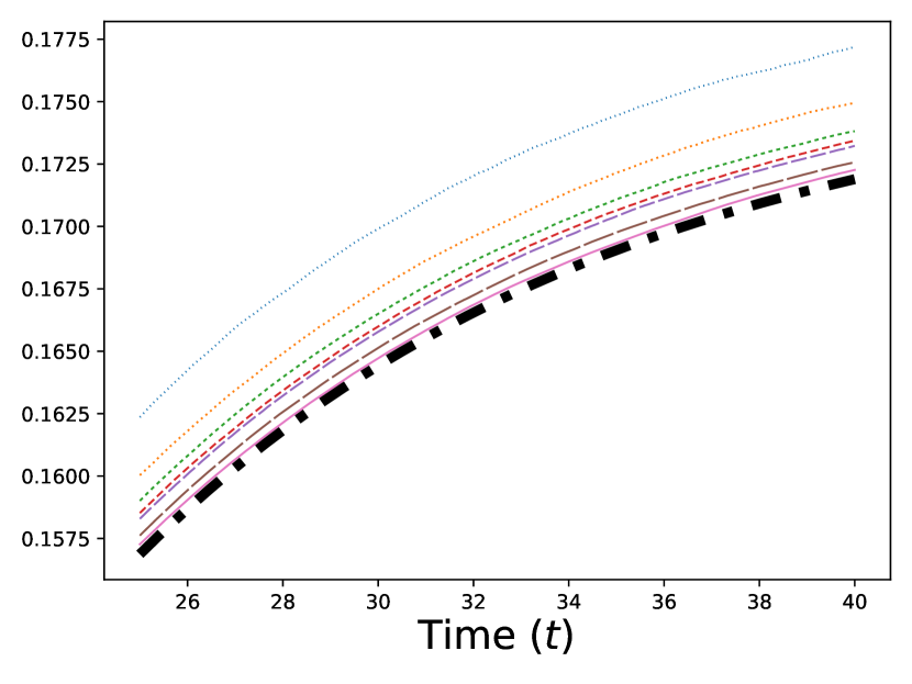
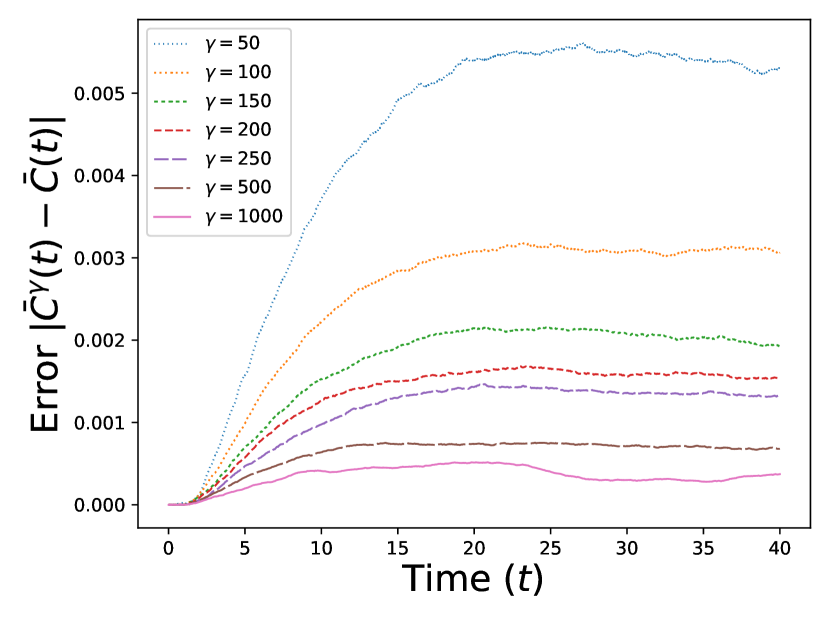
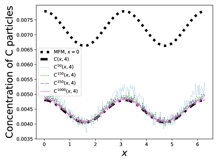
We present the results of our numerical studies in Figure 1. The first three subfigures (top left, top right, and bottom left) each compare the molar mass for the CC particles in the prelimit and limiting processes, denoted by C¯(t)\bar{C}(t) for the MFM and C¯γ(t)\bar{C}^{\gamma}(t) for the CRDME model, over the time interval [0,40][0,40]. The bottom-right subfigure compares the corresponding spatial distributions C(x,t)C(x,t) and Cγ(x,t)C^{\gamma}(x,t) at time t=4t=4.

For the MFM, the molar mass

C¯(t)=02πC(x,t)𝑑x\bar{C}(t)=\int_{0}^{2\pi}C(x,t)dx

is approximated from the spatial distribution C(x,t)C(x,t) at a series of discrete times tt by applying the trapezoidal rule to the numerically computed mean field solution. For the CRDME model, we compute C¯γ(t)\bar{C}^{\gamma}(t) by first averaging the number of particles in each voxel over 280,000 simulations to obtain C¯iγ(t)\bar{C}^{\gamma}_{i}(t), i=1,,Ni=1,...,N, at a series of discrete times tt. Then, the concentration fields Cγ(x,t)C^{\gamma}(x,t) shown in the bottom-right panel of Figure 1 can be computed from C¯iγ(t)\bar{C}^{\gamma}_{i}(t) as the piecewise-linear interpolant of the grid function Cγ(xi,t)=C¯iγ(t)hγC^{\gamma}(x_{i},t)=\frac{\bar{C}^{\gamma}_{i}(t)}{h\gamma}. Finally, the molar mass C¯γ(t)\bar{C}^{\gamma}(t) is computed from Cγ(x,t)C^{\gamma}(x,t) as

C¯γ(t)=i=1NhCγ(xi,t).\bar{C}^{\gamma}(t)=\sum_{i=1}^{N}hC^{\gamma}(x_{i},t).

Refer to caption

(a) Convergence of the CRDME molar mass C¯γ(t)\bar{C}^{\gamma}(t) to the MFM molar mass C¯(t)\bar{C}(t) as γ\gamma increases over the time interval [0,40][0,40], compared with the MFM molar mass in the no-potentials case (κ=0\kappa=0).

Refer to caption


(b) Convergence of the CRDME molar mass C¯γ(t)\bar{C}^{\gamma}(t) to the MFM molar mass C¯(t)\bar{C}(t) as γ\gamma increases over the restricted time interval [25,40][25,40].

Refer to caption

(c) Absolute differences |C¯γ(t)C¯(t)||\bar{C}^{\gamma}(t)-\bar{C}(t)| of the CRDME molar mass C¯γ(t)\bar{C}^{\gamma}(t) and the MFM molar mass C¯(t)\bar{C}(t) on the interval [0,40][0,40] for different values of γ\gamma.

Refer to caption

(d) Comparison of the spatial distribution of the MFM, C(x,t)C(x,t), to the spatial distribution of the CRDME, Cγ(x,t)C^{\gamma}(x,t), at the time t=4t=4, along with the spatial distribution of the MFM in the purely-diffusive (i.e. no potentials) case.
Figure 1. Comparison of the CRDME and MFM solutions. The CRDME data are obtained by averaging the results of 280,000 simulations.

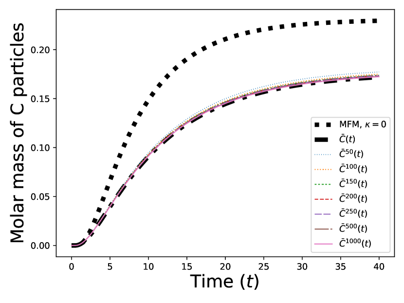
Starting with the top-left panel in Figure 1, we observe that, as expected, the CRDME molar masses C¯γ(t)\bar{C}^{\gamma}(t) converge to the MFM molar masses as γ\gamma\to\infty. We have also included for comparsion the mean-field solution in the no-potentials case (i.e., κ=0\kappa=0), observing that over time, the repulsive pair potential force reduces the effective forward reaction rate (relative to the backward), resulting in a significantly smaller molar mass at the final time.

The top-right and bottom-left panels further compare the molar masses C¯(t)\bar{C}(t) and C¯γ(t)\bar{C}^{\gamma}(t) for the MFM and CRDME models in the κ=200\kappa=200 case; the top-right panel shows a zoomed-in version of the top-left panel, with the κ=0\kappa=0 solution removed and the time interval restricted to [25,40][25,40]. We see more clearly the convergence of the CRDME molar masses C¯γ(t)\bar{C}^{\gamma}(t) to the MFM molar masses C¯(t)\bar{C}(t). Looking directly at the errors in the bottom-left panel, computed as |C¯(t)C¯γ(t)||\bar{C}(t)-\bar{C}^{\gamma}(t)| for each time tt, we see that the maximum errors range from .005\approx.005 (\approx 3%) for γ=50\gamma=50 to .00025\approx.00025 (\approx .15%) for γ=1000\gamma=1000.

Finally, in the bottom right figure, we compare the spatial distribution Cγ(x,t)C^{\gamma}(x,t) for the CRDME model with the MFM spatial distribution C(x,t)C(x,t). Although the CRDME spatial distributions appear significantly noisier than the molar masses due to the relatively small number of particles in each voxel, we can still see that the MFM gives a good fit for the particle model, especially for larger values of γ\gamma. We have also once again included for comparison the κ=0\kappa=0 MFM spatial distribution.

8. Proof of Theorem 5.1.

Without loss of generality, we assume that L~=0\tilde{L}=0 in this section. The case when L~>0\tilde{L}>0 follows by similar arguments as we now give in the L~=0\tilde{L}=0 case.

To rigorously determine the large population limit of the MVSP, we use the martingale problem approach for studying solutions to stochastic differential equations developed by Stroock and Varadhan [12, 46]. The proof is divided into four subsections. In Subsection 8.1, we provide the path level description of μtζ,j\mu_{t}^{\zeta,j}, and we derive equations for its expectation in Subsection 8.2. Tightness and identification of the limit are presented in Subsection 8.3. Lastly, we prove in Subsection 8.4 that the limit equation has a unique solution. Collectively, these results imply Theorem 5.1, see, for example, the proof of Theorem 5.5 in [28] for details.

8.1. Path level description.

For a test function fCb2(d)f\in C_{b}^{2}(\mathbb{R}^{d}) and for each species j=1,,Jj=1,\cdots,J, we obtain the coupled system

f,\displaystyle\langle f, μtζ,j=f,μ0ζ,j+1γi10t1{iγ1,μsζ,j}2DjfQ(Hi(γμsζ,j))dWsi\displaystyle\mu_{t}^{\zeta,j}\rangle=\langle f,\mu_{0}^{\zeta,j}\rangle+\frac{1}{\gamma}\sum_{i\geq 1}\int_{0}^{t}1_{\{i\leq\gamma\langle 1,\mu_{s^{-}}^{\zeta,j}\rangle\}}\sqrt{2D_{j}}\frac{\partial f}{\partial Q}(H^{i}(\gamma\mu_{s^{-}}^{\zeta,j})\bigr{)}dW_{s}^{i}
+1γ0ti=1γ1,μsζ,j(Dj2fQ2(Hi(γμsζ,j))fQ(Hi(γμsζ,j))vj(Hi(γμsζ,j)))ds\displaystyle\phantom{=}+\frac{1}{\gamma}\int_{0}^{t}\sum_{i=1}^{\gamma\langle 1,\mu_{s^{-}}^{\zeta,j}\rangle}\biggl{(}D_{j}\frac{\partial^{2}f}{\partial Q^{2}}\bigl{(}H^{i}(\gamma\mu_{s^{-}}^{\zeta,j})\bigr{)}-\frac{\partial f}{\partial Q}\bigl{(}H^{i}(\gamma\mu_{s^{-}}^{\zeta,j})\bigr{)}\cdot\nabla v_{j}\bigl{(}H^{i}(\gamma\mu_{s^{-}}^{\zeta,j})\bigr{)}\biggr{)}ds
1γ0ti=1γ1,μsζ,j(fQ(Hi(γμsζ,j))1γj=1,jjJk=1γ1,μsζ,juj,j(Hi(γμsζ,j)Hk(γμsζ,j)))ds\displaystyle\phantom{=}-\frac{1}{\gamma}\int_{0}^{t}\sum_{i=1}^{\gamma\langle 1,\mu_{s^{-}}^{\zeta,j}\rangle}\biggl{(}\frac{\partial f}{\partial Q}\bigl{(}H^{i}(\gamma\mu_{s^{-}}^{\zeta,j})\bigr{)}\cdot\frac{1}{\gamma}\nabla\sum_{j^{\prime}=1,j^{\prime}\neq j}^{J}\sum_{k=1}^{\gamma\langle 1,\mu_{s^{-}}^{\zeta,j^{\prime}}\rangle}u_{j,j^{\prime}}\bigl{(}\|H^{i}(\gamma\mu_{s^{-}}^{\zeta,j})-H^{k}(\gamma\mu_{s^{-}}^{\zeta,j^{\prime}})\|\bigr{)}\biggr{)}ds
1γ0ti=1γ1,μsζ,j(fQ(Hi(γμsζ,j))1γk=1,kiγ1,μsζ,juj,j(Hi(γμsζ,j)Hk(γμsζ,j)))ds\displaystyle\phantom{=}-\frac{1}{\gamma}\int_{0}^{t}\sum_{i=1}^{\gamma\langle 1,\mu_{s^{-}}^{\zeta,j}\rangle}\biggl{(}\frac{\partial f}{\partial Q}\bigl{(}H^{i}(\gamma\mu_{s^{-}}^{\zeta,j})\bigr{)}\cdot\frac{1}{\gamma}\nabla\sum_{k=1,k\neq i}^{\gamma\langle 1,\mu_{s^{-}}^{\zeta,j}\rangle}u_{j,j}\biggl{(}\|H^{i}(\gamma\mu_{s^{-}}^{\zeta,j})-H^{k}(\gamma\mu_{s^{-}}^{\zeta,j})\|\biggr{)}\biggr{)}ds
+=1L0t𝕀()𝕐()+3(f,μsζ,j1γr=1αjδHir(j)(γμsζ,j)+1γr=1βjδyr(j)f,μsζ,j)1{𝒊Ω()(γμsζ)}\displaystyle\phantom{=}+\sum_{\ell=1}^{L}\int_{0}^{t}\int_{\mathbb{I}^{(\ell)}}\int_{\mathbb{Y}^{(\ell)}}\int_{\mathbb{R}_{+}^{3}}\biggl{(}\langle f,\mu_{s^{-}}^{\zeta,j}-\frac{1}{\gamma}\sum_{r=1}^{\alpha_{\ell j}}\delta_{H^{i_{r}^{(j)}}(\gamma\mu_{s^{-}}^{\zeta,j})}+\frac{1}{\gamma}\sum_{r=1}^{\beta_{\ell j}}\delta_{y_{r}^{(j)}}\rangle-\langle f,\mu_{s^{-}}^{\zeta,j}\rangle\biggr{)}1_{\{\bm{i}\in\Omega^{(\ell)}(\gamma\mu_{s^{-}}^{\zeta})\}}
×1{θ1Kγ(𝒫()(γμsζ,𝒊))}1{θ2mη(𝒚|𝒫()(γμsζ,𝒊))}1{θ3πγ(𝒚|𝒙,𝝁sζ(dx))}dN(s,𝒊,𝒚,θ1,θ2,θ3)\displaystyle\phantom{=}\qquad\times 1_{\{\theta_{1}\leq K_{\ell}^{\gamma}\bigl{(}\mathcal{P}^{(\ell)}(\gamma\mu_{s^{-}}^{\zeta},\bm{i})\bigr{)}\}}1_{\{\theta_{2}\leq m_{\ell}^{\eta}(\bm{y}|\mathcal{P}^{(\ell)}(\gamma\mu_{s^{-}}^{\zeta},\bm{i}))\}}1_{\{\theta_{3}\leq\pi_{\ell}^{\gamma}\bigl{(}\bm{y}|\bm{x},\bm{\mu}_{s^{-}}^{\zeta}(dx^{\prime})\bigr{)}\}}dN_{\ell}(s,\bm{i,y},\theta_{1},\theta_{2},\theta_{3})
=f,μ0ζ,j+1γi10t1{iγ1,μsζ,j}2DjfQ(Hi(γμsζ,j))𝑑Wsi\displaystyle=\langle f,\mu_{0}^{\zeta,j}\rangle+\frac{1}{\gamma}\sum_{i\geq 1}\int_{0}^{t}1_{\{i\leq\gamma\langle 1,\mu_{s^{-}}^{\zeta,j}\rangle\}}\sqrt{2D_{j}}\frac{\partial f}{\partial Q}(H^{i}(\gamma\mu_{s^{-}}^{\zeta,j})\bigr{)}dW_{s}^{i}
+1γ0ti=1γ1,μsζ,j(Dj2fQ2(Hi(γμsζ,j))fQ(Hi(γμsζ,j))vj(Hi(γμsζ,j)))ds\displaystyle\phantom{=}+\frac{1}{\gamma}\int_{0}^{t}\sum_{i=1}^{\gamma\langle 1,\mu_{s^{-}}^{\zeta,j}\rangle}\biggl{(}D_{j}\frac{\partial^{2}f}{\partial Q^{2}}\bigl{(}H^{i}(\gamma\mu_{s^{-}}^{\zeta,j})\bigr{)}-\frac{\partial f}{\partial Q}\bigl{(}H^{i}(\gamma\mu_{s^{-}}^{\zeta,j})\bigr{)}\cdot\nabla v_{j}\bigl{(}H^{i}(\gamma\mu_{s^{-}}^{\zeta,j})\bigr{)}\biggr{)}ds
1γ0ti=1γ1,μsζ,j(fQ(Hi(γμsζ,j))1γj=1Jk=1γ1,μsζ,juj,j(Hi(γμsζ,j)Hk(γμsζ,j)))ds\displaystyle\phantom{=}-\frac{1}{\gamma}\int_{0}^{t}\sum_{i=1}^{\gamma\langle 1,\mu_{s^{-}}^{\zeta,j}\rangle}\biggl{(}\frac{\partial f}{\partial Q}\bigl{(}H^{i}(\gamma\mu_{s^{-}}^{\zeta,j})\bigr{)}\cdot\frac{1}{\gamma}\nabla\sum_{j^{\prime}=1}^{J}\sum_{k=1}^{\gamma\langle 1,\mu_{s^{-}}^{\zeta,j^{\prime}}\rangle}u_{j,j^{\prime}}\bigl{(}\|H^{i}(\gamma\mu_{s^{-}}^{\zeta,j})-H^{k}(\gamma\mu_{s^{-}}^{\zeta,j^{\prime}})\|\bigr{)}\biggr{)}ds
+1γ0ti=1γ1,μsζ,j(fQ(Hi(γμsζ,j))1γuj,j0)ds\displaystyle\phantom{=}+\frac{1}{\gamma}\int_{0}^{t}\sum_{i=1}^{\gamma\langle 1,\mu_{s^{-}}^{\zeta,j}\rangle}\biggl{(}\frac{\partial f}{\partial Q}\bigl{(}H^{i}(\gamma\mu_{s^{-}}^{\zeta,j})\bigr{)}\cdot\frac{1}{\gamma}\nabla u_{j,j}\|0\|\biggr{)}ds
+1γ=1L0t𝕀()𝕐()+3(f,r=1αjδHir(j)(γμsζ,j)+r=1βjδyr(j))1{𝒊Ω()(γμsζ)}\displaystyle\phantom{=}+\frac{1}{\gamma}\sum_{\ell=1}^{L}\int_{0}^{t}\int_{\mathbb{I}^{(\ell)}}\int_{\mathbb{Y}^{(\ell)}}\int_{\mathbb{R}_{+}^{3}}\biggl{(}\langle f,-\sum_{r=1}^{\alpha_{\ell j}}\delta_{H^{i_{r}^{(j)}}(\gamma\mu_{s^{-}}^{\zeta,j})}+\sum_{r=1}^{\beta_{\ell j}}\delta_{y_{r}^{(j)}}\rangle\biggr{)}1_{\{\bm{i}\in\Omega^{(\ell)}(\gamma\mu_{s^{-}}^{\zeta})\}}
(23) ×1{θ1Kγ(𝒫()(γμsζ,𝒊))}1{θ2mη(𝒚|𝒫()(γμsζ,𝒊))}1{θ3πγ(𝒚|𝒙,μsζ(dx))}dN(s,𝒊,𝒚,θ1,θ2,θ3).\displaystyle\phantom{=}\quad\times 1_{\{\theta_{1}\leq K_{\ell}^{\gamma}\bigl{(}\mathcal{P}^{(\ell)}(\gamma\mu_{s^{-}}^{\zeta},\bm{i})\bigr{)}\}}1_{\{\theta_{2}\leq m_{\ell}^{\eta}(\bm{y}|\mathcal{P}^{(\ell)}(\gamma\mu_{s^{-}}^{\zeta},\bm{i}))\}}1_{\{\theta_{3}\leq\pi_{\ell}^{\gamma}\bigl{(}\bm{y}|\bm{x},\mu_{s^{-}}^{\zeta}(dx^{\prime})\bigr{)}\}}dN_{\ell}(s,\bm{i,y},\theta_{1},\theta_{2},\theta_{3}).

The exchangeability of the sum, the differentiation, and the Lebesgue integral here and in the next subsection are justified by the fact that for fixed ζ,γ1,μsζ,j\zeta,\gamma\langle 1,\mu_{s^{-}}^{\zeta,j}\rangle is finite by Assumption (4.1), and that ff and its partial derivatives are uniformly bounded.

8.2. Taking expectations.

By taking expectation on (23), we have

𝔼[f,μt𝜻,j]\displaystyle\mathbb{E}[\langle f,\mu_{t}^{\bm{\zeta},j}\rangle] =𝔼[f,μ0ζ,j]+𝔼[0td1γi=1γ1,μsζ,j(Dj2fQ2(x)fQ(x)vj(x))δHi(γμsζ,j)(dx)ds]\displaystyle=\mathbb{E}[\langle f,\mu_{0}^{\zeta,j}\rangle]+\mathbb{E}\biggl{[}\int_{0}^{t}\int_{\mathbb{R}^{d}}\frac{1}{\gamma}\sum_{i=1}^{\gamma\langle 1,\mu_{s^{-}}^{\zeta,j}\rangle}\biggl{(}D_{j}\frac{\partial^{2}f}{\partial Q^{2}}(x)-\frac{\partial f}{\partial Q}(x)\cdot\nabla v_{j}(x)\biggr{)}\delta_{H^{i}(\gamma\mu_{s^{-}}^{\zeta,j})}(dx)ds\biggr{]}
𝔼[1γ0tdi=1γ1,μsζ,jfQ(x)(d1γj=1Jk=1γ1,μsζ,juj,j(xy)δHk(γμsζ,j)(dy))\displaystyle\phantom{=}-\mathbb{E}\biggl{[}\frac{1}{\gamma}\int_{0}^{t}\int_{\mathbb{R}^{d}}\sum_{i=1}^{\gamma\langle 1,\mu_{s^{-}}^{\zeta,j}\rangle}\frac{\partial f}{\partial Q}(x)\biggl{(}\int_{\mathbb{R}^{d}}\frac{1}{\gamma}\nabla\sum_{j^{\prime}=1}^{J}\sum_{k=1}^{\gamma\langle 1,\mu_{s^{-}}^{\zeta,j^{\prime}}\rangle}u_{j,j^{\prime}}(\left\lVert x-y\right\rVert)\delta_{H^{k}(\gamma\mu_{s^{-}}^{\zeta,j^{\prime}})}(dy)\biggr{)}
×δHi(γμsζ,j)(dx)ds]\displaystyle\phantom{=}\qquad\qquad\qquad\qquad\qquad\qquad\qquad\qquad\qquad\qquad\qquad\qquad\qquad\times\delta_{H^{i}(\gamma\mu_{s^{-}}^{\zeta,j})}(dx)ds\biggr{]}
+𝔼[1γ0tdi=1γ1,μsζ,jfQ(x)(1γuj,j(0))δHi(γμsζ,j)(dx)ds]\displaystyle\phantom{=}+\mathbb{E}\biggl{[}\frac{1}{\gamma}\int_{0}^{t}\int_{\mathbb{R}^{d}}\sum_{i=1}^{\gamma\langle 1,\mu_{s^{-}}^{\zeta,j}\rangle}\frac{\partial f}{\partial Q}(x)\cdot\biggl{(}\frac{1}{\gamma}\nabla u_{j,j}(\|0\|)\biggr{)}\delta_{H^{i}(\gamma\mu_{s^{-}}^{\zeta,j})}(dx)ds\biggr{]}
=1L𝔼[0t1γiΩ()(γμsζ)(r=1αjf(Hir(j)(γμsζ,j)))Kγ(𝒫()(γμsζ,𝒊))\displaystyle\phantom{=}-\sum_{\ell=1}^{L}\mathbb{E}\biggl{[}\int_{0}^{t}\frac{1}{\gamma}\sum_{i\in\Omega^{(\ell)}(\gamma\mu_{s^{-}}^{\zeta})}\biggl{(}\sum_{r=1}^{\alpha_{\ell j}}f\bigl{(}H^{i_{r}^{(j)}}(\gamma\mu_{s^{-}}^{\zeta,j})\bigr{)}\biggr{)}K_{\ell}^{\gamma}\bigl{(}\mathcal{P}^{(\ell)}(\gamma\mu_{s^{-}}^{\zeta},\bm{i})\bigr{)}
×(𝕐()mη(𝒚|𝒫()(γμsζ,𝒊))πγ(𝒚|𝒙,𝝁sζ(dx))d𝒚)ds]\displaystyle\phantom{=}\qquad\qquad\qquad\qquad\qquad\qquad\times\biggl{(}\int_{\mathbb{Y}^{(\ell)}}m_{\ell}^{\eta}\bigl{(}\bm{y}|\mathcal{P}^{(\ell)}(\gamma\mu_{s^{-}}^{\zeta},\bm{i})\bigr{)}\pi_{\ell}^{\gamma}\bigl{(}\bm{y}|\bm{x},\bm{\mu}_{s^{-}}^{\zeta}(dx^{\prime})\bigr{)}d\bm{y}\biggr{)}ds\biggr{]}
+=1L𝔼[0t1γiΩ()(γμsζ)Kγ(𝒫()(γμsζ,𝒊))\displaystyle\phantom{=}+\sum_{\ell=1}^{L}\mathbb{E}\biggl{[}\int_{0}^{t}\frac{1}{\gamma}\sum_{i\in\Omega^{(\ell)}(\gamma\mu_{s^{-}}^{\zeta})}K_{\ell}^{\gamma}\bigl{(}\mathcal{P}^{(\ell)}(\gamma\mu_{s^{-}}^{\zeta},\bm{i})\bigr{)}
×(𝕐()(r=1βjf(yr(j)))mη(𝒚|𝒫()(γμsζ,𝒊))πγ(𝒚|𝒙,𝝁sζ(dx))d𝒚)ds]\displaystyle\phantom{=}\qquad\qquad\qquad\times\biggl{(}\int_{\mathbb{Y}^{(\ell)}}\bigl{(}\sum_{r=1}^{\beta_{\ell j}}f(y_{r}^{(j)})\bigr{)}m_{\ell}^{\eta}\bigl{(}\bm{y}|\mathcal{P}^{(\ell)}(\gamma\mu_{s^{-}}^{\zeta},\bm{i})\bigr{)}\pi_{\ell}^{\gamma}\bigl{(}\bm{y}|\bm{x},\bm{\mu}_{s^{-}}^{\zeta}(dx^{\prime})\bigr{)}d\bm{y}\biggr{)}ds\biggr{]}
=𝔼[f,μ0ζ,j]+𝔼[0tDj2fQ2(x)fQvj(x),μsζ,j(dx)𝑑s]\displaystyle=\mathbb{E}[\langle f,\mu_{0}^{\zeta,j}\rangle]+\mathbb{E}\biggl{[}\int_{0}^{t}\langle D_{j}\frac{\partial^{2}f}{\partial Q^{2}}(x)-\frac{\partial f}{\partial Q}\cdot\nabla v_{j}(x),\mu_{s^{-}}^{\zeta,j}(dx)\rangle ds\biggr{]}
+𝔼[0tj=1JfQ(x)uj,j(xy),μsζ,j(dy),μsζ,j(dx)𝑑s]\displaystyle\phantom{=}+\mathbb{E}\biggl{[}\int_{0}^{t}\bigl{\langle}\sum_{j^{\prime}=1}^{J}\langle-\frac{\partial f}{\partial Q}(x)\cdot\nabla u_{j,j^{\prime}}(\left\lVert x-y\right\rVert),\mu_{s^{-}}^{\zeta,j^{\prime}}(dy)\rangle,\mu_{s^{-}}^{\zeta,j}(dx)\bigr{\rangle}ds\biggr{]}
+1γ𝔼[0tfQ(x)uj,j(0),μsζ,j(dx)𝑑s]\displaystyle\phantom{=}+\frac{1}{\gamma}\mathbb{E}\biggl{[}\int_{0}^{t}\langle\frac{\partial f}{\partial Q}(x)\cdot\nabla u_{j,j}(\|0\|),\mu_{s^{-}}^{\zeta,j}(dx)\rangle ds\biggr{]}
=1L𝔼[0t1γ𝕏()iΩ()(γμsζ)(r=1αjf(xr(j)))Kγ(𝒙)\displaystyle\phantom{=}-\sum_{\ell=1}^{L}\mathbb{E}\biggl{[}\int_{0}^{t}\frac{1}{\gamma}\int_{\mathbb{X}^{(\ell)}}\sum_{i\in\Omega^{(\ell)}(\gamma\mu_{s^{-}}^{\zeta})}\bigl{(}\sum_{r=1}^{\alpha_{\ell j}}f(x_{r}^{(j)})\bigr{)}K^{\gamma}_{\ell}(\bm{x})
×(𝕐()mη(𝒚|𝒙)πγ(𝒚|𝒙,𝝁sζ(dx))d𝒚)δ𝒫()(γμsζ,𝒊)(d𝒙)ds]\displaystyle\phantom{=}\qquad\qquad\qquad\qquad\qquad\times\biggl{(}\int_{\mathbb{Y}^{(\ell)}}m_{\ell}^{\eta}(\bm{y}|\bm{x})\pi_{\ell}^{\gamma}\bigl{(}\bm{y}|\bm{x},\bm{\mu}_{s^{-}}^{\zeta}(dx^{\prime})\bigr{)}d\bm{y}\biggr{)}\delta_{\mathcal{P}^{(\ell)}(\gamma\mu_{s^{-}}^{\zeta},\bm{i})}(d\bm{x})ds\biggr{]}
+=1L𝔼[0t1γ𝕏()iΩ()(γμsζ)Kγ(𝒙)\displaystyle\phantom{=}+\sum_{\ell=1}^{L}\mathbb{E}\biggl{[}\int_{0}^{t}\frac{1}{\gamma}\int_{\mathbb{X}^{(\ell)}}\sum_{i\in\Omega^{(\ell)}(\gamma\mu_{s^{-}}^{\zeta})}K^{\gamma}_{\ell}(\bm{x})
×(𝕐()(r=1βjf(yr(j)))mη(𝒚|𝒙)πγ(𝒚|𝒙,𝝁sζ(dx))d𝒚)δ𝒫()(γμsζ,𝒊)(d𝒙)ds].\displaystyle\phantom{=}\qquad\qquad\times\biggl{(}\int_{\mathbb{Y}^{(\ell)}}\bigl{(}\sum_{r=1}^{\beta_{\ell j}}f(y_{r}^{(j)})\bigr{)}m_{\ell}^{\eta}(\bm{y}|\bm{x})\pi_{\ell}^{\gamma}\bigl{(}\bm{y}|\bm{x},\bm{\mu}_{s^{-}}^{\zeta}(dx^{\prime})\bigr{)}d\bm{y}\biggr{)}\delta_{\mathcal{P}^{(\ell)}(\gamma\mu_{s^{-}}^{\zeta},\bm{i})}(d\bm{x})ds\biggr{]}.

Define the operator

(24) Γ,j[f](𝒙,𝒚):=r=1β,jf(yr(j))r=1α,jf(xr(j)),\Gamma^{\ell,j}[f](\bm{x},\bm{y}):=\sum_{r=1}^{\beta_{\ell,j}}f(y_{r}^{(j)})-\sum_{r=1}^{\alpha_{\ell,j}}f(x_{r}^{(j)}),

and note in the remainder that for any test functions we consider

|Γ,j[f](𝒙,𝒚)|(β,j+α,j)f.\left|\Gamma^{\ell,j}[f](\bm{x},\bm{y})\right\rvert\leq(\beta_{\ell,j}+\alpha_{\ell,j})\left\lVert f\right\rVert_{\infty}.

Using the operators (jf)(x)(\mathcal{L}_{j}f)(x) and (~j,jf)(x,y)(\tilde{\mathcal{L}}_{j,j^{\prime}}f)(x,y) defined in (8) we then obtain

𝔼[f,μt𝜻,j]\displaystyle\mathbb{E}[\langle f,\mu_{t}^{\bm{\zeta},j}\rangle] =𝔼[f,μ0ζ,j]+𝔼[0t(jf)(x),μsζ,j(dx)𝑑s]\displaystyle=\mathbb{E}[\langle f,\mu_{0}^{\zeta,j}\rangle]+\mathbb{E}\biggl{[}\int_{0}^{t}\langle(\mathcal{L}_{j}f)(x),\mu_{s^{-}}^{\zeta,j}(dx)\rangle ds\biggr{]}
+𝔼[0tj=1J(~j,jf)(x,y),μsζ,j(dy),μsζ,j(dx)𝑑s]\displaystyle\phantom{=}+\mathbb{E}\biggl{[}\int_{0}^{t}\bigl{\langle}\sum_{j^{\prime}=1}^{J}\langle(\tilde{\mathcal{L}}_{j,j^{\prime}}f)(x,y),\mu_{s^{-}}^{\zeta,j^{\prime}}(dy)\rangle,\mu_{s^{-}}^{\zeta,j}(dx)\bigr{\rangle}ds\biggr{]}
+1γ𝔼[0tfQ(x)uj,j(0),μsζ,j(dx)𝑑s]\displaystyle\phantom{=}+\frac{1}{\gamma}\mathbb{E}\biggl{[}\int_{0}^{t}\langle\frac{\partial f}{\partial Q}(x)\cdot\nabla u_{j,j}(\|0\|),\mu_{s^{-}}^{\zeta,j}(dx)\rangle ds\biggr{]}
+=1L𝔼[0t𝕏~()1𝜶()!K(𝒙)(𝕐()Γ,j[f](𝒙,𝒚)mη(𝒚|𝒙)\displaystyle\phantom{=}+\sum_{\ell=1}^{L}\mathbb{E}\biggl{[}\int_{0}^{t}\int_{\tilde{\mathbb{X}}(\ell)}\frac{1}{\bm{\alpha}^{(\ell)}!}K_{\ell}(\bm{x})\biggl{(}\int_{\mathbb{Y}^{(\ell)}}\Gamma^{\ell,j}[f](\bm{x},\bm{y}){m_{\ell}^{\eta}(\bm{y}|\bm{x})}
(25) ×πγ(𝒚|𝒙,𝝁sζ(dx))d𝒚)λ()[μsζ](d𝒙)ds].\displaystyle\phantom{=}\qquad\qquad\qquad\qquad\qquad\qquad\qquad\times\pi_{\ell}^{\gamma}\bigl{(}\bm{y}|\bm{x},\bm{\mu}_{s^{-}}^{\zeta}(dx^{\prime})\bigr{)}d\bm{y}\biggr{)}\lambda^{(\ell)}[\mu_{s^{-}}^{\zeta}](d\bm{x})ds\biggr{]}.

For this last equality, we switch integrals of the form 𝕏()iΩ()(γμsζ)δ𝒫()(γμsζ,i)(d𝒙)\int_{\mathbb{X}^{(\ell)}}\sum_{i\in\Omega^{(\ell)}(\gamma\mu_{s-}^{\zeta})}\cdots\delta_{\mathcal{P}^{(\ell)}(\gamma\mu_{s-}^{\zeta},i)}(d\bm{x}) to 𝕏~()1α()!λ()[μsζ](d𝒙)\int_{\tilde{\mathbb{X}}^{(\ell)}}\frac{1}{\alpha^{(\ell)}!}\cdots\lambda^{(\ell)}[\mu_{s-}^{\zeta}](d\bm{x}) using the definitions of μsζ,j(d𝒙)\mu_{s}^{\zeta,j}(d\bm{x}) and λ()[]\lambda^{(\ell)}[\cdot] (see equation (6) and Definition 2.6), and removing probability zero sets where two particles with the same type are simultaneously located at the same spatial location (see Definition 2.7). Note that by definition indices for particles of the same species are ordered by the allowable substrate index sampling space Ω()\Omega^{(\ell)} (see Definition 2.5). In converting from integrals involving the positions of individual particles with δ𝒫()(γμsζ,i)(d𝒙)\delta_{\mathcal{P}^{(\ell)}(\gamma\mu_{s-}^{\zeta},i)}(d\bm{x}) to integrals involving product measures λ()[μsζ](d𝒙)\lambda^{(\ell)}[\mu_{s-}^{\zeta}](d\bm{x}), we need to remove the “diagonal” indices by means of integrating on 𝕏~()\tilde{\mathbb{X}}^{(\ell)} (see Definition 2.7) and normalizing by the total number of index orderings 𝜶()!\bm{\alpha}^{(\ell)}!.

8.3. Tightness and Identification of the limit.

We start by discussing relative compactness of the sequence {μtζ,j}t[0,T],j=1,2,,J\{\mu_{t}^{\zeta,j}\}_{t\in[0,T]},j=1,2,\cdots,J. Recall that MF(d)M_{F}(\mathbb{R}^{d}) denotes the space of finite measures endowed with the weak topology.

Lemma 8.1.

The measure-valued processes {μtζ,j}t[0,T],j=1,2,,J\{\mu_{t}^{\zeta,j}\}_{t\in[0,T]},j=1,2,\cdots,J are relatively compact on 𝔻MF(d)[0,T]\mathbb{D}_{M_{F}(\mathbb{R}^{d})}[0,T], the space of càdlàg paths with values in MF(d)M_{F}(\mathbb{R}^{d}) endowed with Skorokhod topology. Further, the corresponding weak limit of any convergent subsequence of {𝛍tζ}t[0,T]\{\bm{\mu}^{\zeta}_{t}\}_{t\in[0,T]} as ζ0\zeta\to 0 is in Cj=1JMF(d)([0,T])C_{\otimes_{j=1}^{J}M_{F}(\mathbb{R}^{d})}([0,T]).

Proof.

The proof is exactly as in [28] with minor adjustments to account for the presence of the bounded one-body and two-body potential interactions. We omit the details for the sake of brevity. ∎

Given a sequence ζk0\zeta_{k}\to 0 as kk\to\infty, by Lemma 8.1 the sequence of marginal distribution vectors {𝝁tζk}k\{\bm{\mu}_{t}^{\zeta_{k}}\}_{k} has a weakly convergent subsequence. Recall that we let 𝝃t:=(ξt1,ξt2,,ξtJ)\bm{\xi}_{t}:=(\xi_{t}^{1},\xi_{t}^{2},\cdots,\xi_{t}^{J}) be the corresponding limiting marginal distribution vector on J×d\mathbb{R}^{J\times d} and ξt=j=1JξtjδSj\xi_{t}=\sum_{j=1}^{J}\xi_{t}^{j}\delta_{S_{j}} the corresponding limiting particle distribution on P^\hat{P}. We claim that for each 1jJ1\leq j\leq J, ξtj\xi_{t}^{j} is then the unique solution to (14), which in the case that L~=0\tilde{L}=0 becomes

(26) f,ξtj\displaystyle\langle f,\xi_{t}^{j}\rangle =f,ξ0j+0t(jf)(x),ξsj(dx)𝑑s+0tj=1J(~j,jf)(x,y),ξsj(dy),ξsj(dx)𝑑s\displaystyle=\langle f,\xi_{0}^{j}\rangle+\int_{0}^{t}\langle(\mathcal{L}_{j}f)(x),\xi_{s}^{j}(dx)\rangle ds+\int_{0}^{t}\bigl{\langle}\sum_{j^{\prime}=1}^{J}\langle(\tilde{\mathcal{L}}_{j,j^{\prime}}f)(x,y),\xi_{s}^{j^{\prime}}(dy)\rangle,\xi_{s}^{j}(dx)\bigr{\rangle}ds
+=1L0t𝕏~()1𝜶()!K(𝒙)(𝕐()Γ,j[f](𝒙,𝒚)m(𝒚|𝒙)π(𝒚|𝒙,𝝃s(dx))𝑑𝒚)λ()[ξs](d𝒙)𝑑s,\displaystyle\phantom{=}+\sum_{\ell=1}^{L}\int_{0}^{t}\int_{\tilde{\mathbb{X}}(\ell)}\frac{1}{\bm{\alpha}^{(\ell)}!}K_{\ell}(\bm{x})\biggl{(}\int_{\mathbb{Y}^{(\ell)}}\Gamma^{\ell,j}[f](\bm{x},\bm{y})m_{\ell}(\bm{y}|\bm{x})\pi_{\ell}\bigl{(}\bm{y}|\bm{x},\bm{\xi}_{s}(dx^{\prime})\bigr{)}d\bm{y}\biggr{)}\lambda^{(\ell)}[\xi_{s}](d\bm{x})ds,

where Γ,j\Gamma^{\ell,j} is defined in (24). Uniqueness of solutions to this equation is shown in Subsection 8.4. We now identify that the limit ξtj\xi^{j}_{t} satisfies this equation.

Let 𝒮\mathcal{S} be the collection of elements Φ\Phi in the space of bounded functionals, B(j=1JMF(d))B(\otimes_{j=1}^{J}M_{F}(\mathbb{R}^{d})\bigr{)}, of the form

(27) Φ(𝝁)=φ(f1,𝝁,f2,𝝁fM,𝝁)\Phi(\bm{\mu})=\varphi(\langle f_{1},\bm{\mu}\rangle,\langle f_{2},\bm{\mu}\rangle\ldots\langle f_{M},\bm{\mu}\rangle)

for some MM\in\mathbb{N}, some φC(J×M)\varphi\in C^{\infty}(\mathbb{R}^{J\times M}), and fm,𝝁=(f1,m,μ1,,fJ,m,μJ)\langle f_{m},\bm{\mu}\rangle=(\langle f_{1,m},\mu^{1}\rangle,\cdots,\langle f_{J,m},\mu^{J}\rangle) where each {fj,m}Cb2(d)\{f_{j,m}\}\in C_{b}^{2}(\mathbb{R}^{d}) for j=1,,Jj=1,\cdots,J and m=1,,Mm=1,\cdots,M. Then 𝒮\mathcal{S} separates points in j=1JMF(d)\otimes_{j=1}^{J}M_{F}(\mathbb{R}^{d}) (see Chapter 3.43.4 of [12] and Proposition 3.33.3 of [5]). To identify the limit, it suffices to show convergence of the martingale problem for functions of the form (27), given the existence and uniqueness of the limiting process.

For Φ𝒮\Phi\in\mathcal{S} of the form (27),𝝁:=(μ1,μ2,μJ)j=1JMF(d)\eqref{mar},\bm{\mu}:=(\mu^{1},\mu^{2}\cdots,\mu^{J})\in\otimes_{j=1}^{J}M_{F}(\mathbb{R}^{d}) and μ=j=1JμjδSjMF(P^)\mu=\sum_{j=1}^{J}\mu^{j}\delta_{S_{j}}\in M_{F}(\hat{P}) with each μjMF(d)\mu^{j}\in M_{F}(\mathbb{R}^{d}), the generator 𝒜\mathcal{A} of (26) and of the limiting martingale problem for 1jJ1\leq j\leq J, is defined as

(𝒜Φ)(𝝁)\displaystyle(\mathcal{A}\Phi)(\bm{\mu}) m=1Mj=1Jφx(m1)J+j(f1,𝝁,f2,𝝁fM,𝝁)\displaystyle\coloneqq\sum_{m=1}^{M}\sum_{j=1}^{J}\frac{\partial\varphi}{\partial x_{(m-1)*J+j}}(\langle f_{1},\bm{\mu}\rangle,\langle f_{2},\bm{\mu}\rangle\ldots\langle f_{M},\bm{\mu}\rangle)
×[(jfj,m)(x),μj(dx)+j=1J~j,jfj,m(x,y),μj(dy),μj(dx)\displaystyle\times\biggl{[}\langle(\mathcal{L}_{j}f_{j,m})(x),\mu^{j}(dx)\rangle+\bigl{\langle}\sum_{j^{\prime}=1}^{J}\langle\tilde{\mathcal{L}}_{j,j^{\prime}}f_{j,m}(x,y),\mu^{j^{\prime}}(dy)\rangle,\mu^{j}(dx)\bigr{\rangle}
+=1L𝕏~()1𝜶()!K(𝒙)(𝕐()Γ,j[fj,m](𝒙,𝒚)m(𝒚|𝒙)π(𝒚|𝒙,𝝁(dx))d𝒚)λ()[μ](d𝒙)].\displaystyle+\sum_{\ell=1}^{L}\int_{\tilde{\mathbb{X}}(\ell)}\frac{1}{\bm{\alpha}^{(\ell)}!}K_{\ell}(\bm{x})\biggl{(}\int_{\mathbb{Y}^{(\ell)}}\Gamma^{\ell,j}[f_{j,m}](\bm{x},\bm{y})m_{\ell}(\bm{y}|\bm{x})\pi_{\ell}\bigl{(}\bm{y}|\bm{x},\bm{\mu}(dx^{\prime})\bigr{)}d\bm{y}\biggr{)}\lambda^{(\ell)}[\mu](d\bm{x})\biggr{]}.
Lemma 8.2.

(Weak Convergence). For any Φ𝒮\Phi\in\mathcal{S} and 0r1r2rW=s<t<T0\leq r_{1}\leq r_{2}\cdots\leq r_{W}=s<t<T and {ψw}w=1W\{\psi_{w}\}_{w=1}^{W}\subset B(j=1JMF(d))B(\otimes_{j=1}^{J}M_{F}(\mathbb{R}^{d})\bigr{)}, we have that

(28) limζ0𝔼[{Φ(𝝁tζ)Φ(μsζ)st(𝒜Φ)(𝝁rζ)𝑑r}w=1Wψw(𝝁rwζ)]=0.\lim_{\zeta\rightarrow 0}\mathbb{E}\biggl{[}\{\Phi(\bm{\mu}_{t}^{\zeta})-\Phi(\mu_{s}^{\zeta})-\int_{s}^{t}(\mathcal{A}\Phi)(\bm{\mu}_{r}^{\zeta})dr\}\prod_{w=1}^{W}\psi_{w}(\bm{\mu}_{r_{w}}^{\zeta})\biggr{]}=0.
Proof.

For each j=1,Jj=1,\cdots J, we can rewrite (7) as

f,μtζ,j=f,μ0ζ,j+Mtf,j+Atf,j\langle f,\mu_{t}^{\zeta,j}\rangle=\langle f,\mu_{0}^{\zeta,j}\rangle+M_{t}^{f,j}+A_{t}^{f,j}

where

Atf,j\displaystyle A_{t}^{f,j} =0t(jf)(x),μsζ,j(dx)𝑑s+0tj=1J(~j,jf)(x,y),μsζ,j(dy),μsζ,j(dx)𝑑s\displaystyle=\int_{0}^{t}\langle(\mathcal{L}_{j}f)(x),\mu_{s-}^{\zeta,j}(dx)\rangle ds+\int_{0}^{t}\bigl{\langle}\sum_{j^{\prime}=1}^{J}\langle(\tilde{\mathcal{L}}_{j,j^{\prime}}f)(x,y),\mu_{s-}^{\zeta,j^{\prime}}(dy)\rangle,\mu_{s-}^{\zeta,j}(dx)\bigr{\rangle}ds
+1γ0tfQ(x)uj,j(0),μsζ,j(dx)𝑑s\displaystyle\phantom{=}+\frac{1}{\gamma}\int_{0}^{t}\langle\frac{\partial f}{\partial Q}(x)\cdot\nabla u_{j,j}(\|0\|),\mu_{s-}^{\zeta,j}(dx)\rangle ds
+=1L0t𝕏~()1𝜶()!K(𝒙)(𝕐()Γ,j[f](𝒙,𝒚)mη(𝒚|𝒙)πγ(𝒚|𝒙,𝝁sζ(dx))𝑑𝒚)λ()[μsζ](d𝒙)𝑑s\displaystyle\phantom{=}+\sum_{\ell=1}^{L}\int_{0}^{t}\int_{\tilde{\mathbb{X}}(\ell)}\frac{1}{\bm{\alpha}^{(\ell)}!}K_{\ell}(\bm{x})\biggl{(}\int_{\mathbb{Y}^{(\ell)}}\Gamma^{\ell,j}[f](\bm{x},\bm{y}){m_{\ell}^{\eta}(\bm{y}|\bm{x})}\pi_{\ell}^{\gamma}\bigl{(}\bm{y}|\bm{x},\bm{\mu}_{s-}^{\zeta}(dx^{\prime})\bigr{)}d\bm{y}\biggr{)}\lambda^{(\ell)}[\mu_{s-}^{\zeta}](d\bm{x})ds

and

Mtf,j\displaystyle M_{t}^{f,j} =1γi10t1{iγ1,μsζ,j}2DjfQ(Hi(γμsζ,j))𝑑Wsi\displaystyle=\frac{1}{\gamma}\sum_{i\geq 1}\int_{0}^{t}1_{\{i\leq\gamma\langle 1,\mu_{s-}^{\zeta,j}\rangle\}}\sqrt{2D_{j}}\frac{\partial f}{\partial Q}\bigl{(}H^{i}(\gamma\mu_{s-}^{\zeta,j})\bigr{)}dW_{s}^{i}
+1γ=1L0t𝕀()𝕐()+3(f,r=1αjδH(j)(γμsζ,j)+r=1β,jδyr(j))1{𝒊Ω()(γμsζ)}\displaystyle\phantom{=}+\frac{1}{\gamma}\sum_{\ell=1}^{L}\int_{0}^{t}\int_{\mathbb{I}^{(\ell)}}\int_{\mathbb{Y}^{(\ell)}}\int_{\mathbb{R}_{+}^{3}}\biggl{(}\langle f,-\sum_{r=1}^{\alpha_{\ell j}}\delta_{H^{(j)}}(\gamma\mu_{s-}^{\zeta,j})+\sum_{r=1}^{\beta_{\ell,j}}\delta_{y_{r}^{(j)}}\rangle\biggr{)}1_{\{\bm{i}\in\Omega^{(\ell)}(\gamma\mu_{s-}^{\zeta})\}}
×1{θ1Kγ(𝒫()(γμsζ,𝒊))}1{θ2mη(𝒚|𝒫()(γμsζ,𝒊))}1{θ3πγ(𝒚|𝒙,𝝁sζ(dx))}dN~(s,𝒊,𝒚,θ1,θ2,θ3).\displaystyle\phantom{=}\times 1_{\{\theta_{1}\leq K_{\ell}^{\gamma}(\mathcal{P}^{(\ell)}(\gamma\mu_{s-}^{\zeta},\bm{i})\bigr{)}\}}1_{\{\theta_{2}\leq m_{\ell}^{\eta}(\bm{y}|\mathcal{P}^{(\ell)}(\gamma\mu_{s-}^{\zeta},\bm{i})\bigr{)}\}}1_{\{\theta_{3}\leq\pi_{\ell}^{\gamma}\bigl{(}\bm{y}|\bm{x},\bm{\mu}_{s^{-}}^{\zeta}(dx^{\prime})\bigr{)}\}}d\tilde{N}_{\ell}(s,\bm{i,y},\theta_{1},\theta_{2},\theta_{3}).

Note that Mtf,jM_{t}^{f,j} is a square integrable martingale (see Proposition 2.42.4 in [24]) with quadratic variation

Mf,jt\displaystyle\langle M^{f,j}\rangle_{t} =1γ20ti=1γ1,μsζ,j(2DjfQ(Hi(γμsζ,j)))2ds\displaystyle=\frac{1}{\gamma^{2}}\int_{0}^{t}\sum_{i=1}^{\gamma\langle 1,\mu_{s-}^{\zeta,j}\rangle}\biggl{(}\sqrt{2D_{j}}\frac{\partial f}{\partial Q}\bigl{(}H^{i}(\gamma\mu_{s-}^{\zeta,j})\bigr{)}\biggr{)}^{2}ds
+1γ2=1L0t𝕐(){iΩ()(γμs)ζ)}(r=1αjf(Hirj(γμsζ,j))+r=1βjf(yrj))2\displaystyle\phantom{=}+\frac{1}{\gamma^{2}}\sum_{\ell=1}^{L}\int_{0}^{t}\int_{\mathbb{Y}^{(\ell)}}\sum_{\{i\in\Omega^{(\ell)}(\gamma\mu_{s-)}^{\zeta})\}}\biggl{(}-\sum_{r=1}^{\alpha_{\ell j}}f\bigl{(}H^{i_{r}^{j}}(\gamma\mu_{s-}^{\zeta,j})\bigr{)}+\sum_{r=1}^{\beta_{\ell j}}f(y_{r}^{j})\biggr{)}^{2}
×Kγ(𝒫()(γμsζ,𝒊))mη(𝒚|𝒫()(γμsζ,𝒊))πγ(𝒚|𝒙,𝝁sζ(dx))d𝒚ds\displaystyle\phantom{=}\qquad\qquad\qquad\qquad\times K_{\ell}^{\gamma}\bigl{(}\mathcal{P}^{(\ell)}(\gamma\mu_{s-}^{\zeta},\bm{i})\bigr{)}m_{\ell}^{\eta}\bigl{(}\bm{y}|\mathcal{P}^{(\ell)}(\gamma\mu_{s-}^{\zeta},\bm{i})\bigr{)}\pi_{\ell}^{\gamma}\bigl{(}\bm{y}|\bm{x},\bm{\mu}_{s^{-}}^{\zeta}(dx^{\prime})\bigr{)}d\bm{y}\,ds

The quadratic variation of Mtf,jM_{t}^{f,j} is thus uniformly bounded and goes to 0 as ζ0\zeta\rightarrow 0, due to the uniform boundedness of ff and its partial derivatives, and by Assumptions 4.4 and 4.6.

Now define Mtf,j=𝒞tf,j+𝒟tf,jM_{t}^{f,j}=\mathcal{C}_{t}^{f,j}+\mathcal{D}_{t}^{f,j}, where

𝒞tf,j=1γi10t1{iγ1,μsζ,j}2DjfQ(Hi(γμsζ,j))𝑑Wsi\mathcal{C}_{t}^{f,j}=\frac{1}{\gamma}\sum_{i\geq 1}\int_{0}^{t}1_{\{i\leq\gamma\langle 1,\mu_{s-}^{\zeta,j}\rangle\}}\sqrt{2D_{j}}\frac{\partial f}{\partial Q}\bigl{(}H^{i}(\gamma\mu_{s-}^{\zeta,j})\bigr{)}dW_{s}^{i}

is the continuous martingale part, and

(29) 𝒟tf,j\displaystyle\mathcal{D}_{t}^{f,j} =1γ=1L0t𝕀()𝕐()+3(f,r=1αjδHir(j)(γμsζ,j)+r=1βjδyr(j))1{𝒊Ω()(γμsζ)}\displaystyle=\frac{1}{\gamma}\sum_{\ell=1}^{L}\int_{0}^{t}\int_{\mathbb{I}^{(\ell)}}\int_{\mathbb{Y}^{(\ell)}}\int_{\mathbb{R}_{+}^{3}}\biggl{(}\langle f,-\sum_{r=1}^{\alpha_{\ell j}}\delta_{H^{i_{r}^{(j)}}(\gamma\mu_{s-}^{\zeta,j})}+\sum_{r=1}^{\beta_{\ell j}}\delta_{y_{r}^{(j)}}\rangle\biggr{)}1_{\{\bm{i}\in\Omega^{(\ell)}(\gamma\mu_{s-}^{\zeta})\}}
×1{θ1Kγ(𝒫()(γμsζ,i))}1{θ2mη(𝒚|𝒫()(γμsζ,i))}1{θ3πγ(𝒚|𝒙,𝝁sζ(dx))}dN~(s,𝒊,𝒚,θ1,θ2,θ3),\displaystyle\phantom{=}\times 1_{\{\theta_{1}\leq K_{\ell}^{\gamma}\bigl{(}\mathcal{P}^{(\ell)}(\gamma\mu_{s-}^{\zeta},i)\bigr{)}\}}1_{\{\theta_{2}\leq m_{\ell}^{\eta}\bigl{(}\bm{y}|\mathcal{P}^{(\ell)}(\gamma\mu_{s-}^{\zeta},i)\bigr{)}\}}1_{\{\theta_{3}\leq\pi_{\ell}^{\gamma}\bigl{(}\bm{y}|\bm{x},\bm{\mu}_{s^{-}}^{\zeta}(dx^{\prime})\bigr{)}\}}d\tilde{N}_{\ell}(s,\bm{i},\bm{y},\theta_{1},\theta_{2},\theta_{3}),

is the martingale part coming from the stochastic integral with respect to the Poisson point processes.

Let θ=(θ1,θ2,θ3)\theta=(\theta_{1},\theta_{2},\theta_{3}). For simplicity of notation, we define

g,f,μζ,j(s,𝒊,𝒚,θ)\displaystyle g^{\ell,f,\mu^{\zeta,j}}(s,\bm{i},\bm{y},\theta) =(f,μsζ,j1γr=1αjδHir(j)(γμsζ,j)+1γr=1βjδyr(j)f,μs𝜻,j)1{𝒊Ω()(γμsζ)}\displaystyle=\biggl{(}\langle f,\mu_{s-}^{\zeta,j}-\frac{1}{\gamma}\sum_{r=1}^{\alpha_{\ell j}}\delta_{H^{i_{r}^{(j)}}(\gamma\mu_{s-}^{\zeta,j})}+\frac{1}{\gamma}\sum_{r=1}^{\beta_{\ell j}}\delta_{y_{r}^{(j)}}\rangle-\langle f,\mu_{s-}^{\bm{\zeta},j}\rangle\biggr{)}1_{\{\bm{i}\in\Omega^{(\ell)}(\gamma\mu_{s-}^{\zeta})\}}
×1{θ1Kγ(𝒫()(γμsζ,i))}1{θ2mη(𝒚|𝒫()(γμsζ,i))}1{θ3πγ(𝒚|𝒙,𝝁sζ(dx))}\displaystyle\phantom{=}\qquad\qquad\times 1_{\{\theta_{1}\leq K_{\ell}^{\gamma}\bigl{(}\mathcal{P}^{(\ell)}(\gamma\mu_{s-}^{\zeta},i)\bigr{)}\}}1_{\{\theta_{2}\leq m_{\ell}^{\eta}\bigl{(}\bm{y}|\mathcal{P}^{(\ell)}(\gamma\mu_{s-}^{\zeta},i)\bigr{)}\}}1_{\{\theta_{3}\leq\pi_{\ell}^{\gamma}\bigl{(}\bm{y}|\bm{x},\bm{\mu}_{s^{-}}^{\zeta}(dx^{\prime})\bigr{)}\}}
=1γ(r=1αjf(Hir(j)(γμsζ,j))+r=1βjf(yr(j)))1{𝒊Ω()(γμsζ)}1{θ1Kγ(𝒫()(γμsζ,i))}\displaystyle=\frac{1}{\gamma}\biggl{(}-\sum_{r=1}^{\alpha_{\ell j}}f\left(H^{i_{r}^{(j)}}(\gamma\mu_{s-}^{\zeta,j})\right)+\sum_{r=1}^{\beta_{\ell j}}f(y_{r}^{(j)})\biggr{)}1_{\{\bm{i}\in\Omega^{(\ell)}(\gamma\mu_{s-}^{\zeta})\}}1_{\{\theta_{1}\leq K_{\ell}^{\gamma}\bigl{(}\mathcal{P}^{(\ell)}(\gamma\mu_{s-}^{\zeta},i)\bigr{)}\}}
×1{θ2mη(𝒚|𝒫()(γμsζ,i))}1{θ3πγ(𝒚|𝒙,𝝁sζ(dx))},\displaystyle\phantom{=}\qquad\qquad\qquad\qquad\qquad\qquad\times 1_{\{\theta_{2}\leq m_{\ell}^{\eta}\bigl{(}\bm{y}|\mathcal{P}^{(\ell)}(\gamma\mu_{s-}^{\zeta},i)\bigr{)}\}}1_{\{\theta_{3}\leq\pi_{\ell}^{\gamma}\bigl{(}\bm{y}|\bm{x},\bm{\mu}_{s^{-}}^{\zeta}(dx^{\prime})\bigr{)}\}},

which represents the jumps and is uniformly bounded by 𝒪(1γ)\mathcal{O}(\frac{1}{\gamma}). With some abuse of notation we shall write 𝒈,f,𝝁ζ\bm{g}^{\ell,f,\bm{\mu}^{\zeta}} for the vector (g,f,μζ,1,,g,f,μζ,J)(g^{\ell,f,\mu^{\zeta,1}},\cdots,g^{\ell,f,\mu^{\zeta,J}}). Then (29) becomes

𝒟tf,j==1L0t𝕀()𝕐()+3g,f,μζ,j(s,𝒊,𝒚,θ)𝑑N~(s,𝒊,𝒚,θ1,θ2,θ3).\mathcal{D}_{t}^{f,j}=\sum_{\ell=1}^{L}\int_{0}^{t}\int_{\mathbb{I}^{(\ell)}}\int_{\mathbb{Y}^{(\ell)}}\int_{\mathbb{R}_{+}^{3}}g^{\ell,f,\mu^{\zeta,j}}(s,\bm{i},\bm{y},\theta)d\tilde{N}_{\ell}(s,\bm{i},\bm{y},\theta_{1},\theta_{2},\theta_{3}).

Applying Itô’s formula (see Theorem 5.15.1 in [24]) to Φ(𝝁tζ)\Phi(\bm{\mu}_{t}^{\zeta}) we obtain

Φ(𝝁tζ)Φ(𝝁sζ)st(𝒜Φ)(𝝁rζ)𝑑r=stm=1Mj=1Jφx(m1)J+j(f1,𝝁rζ,f2,𝝁rζfM,𝝁rζ)d𝒞rfj,m,j\displaystyle\Phi(\bm{\mu}_{t}^{\zeta})-\Phi(\bm{\mu}_{s}^{\zeta})-\int_{s}^{t}(\mathcal{A}\Phi)(\bm{\mu}_{r}^{\zeta})dr=\int_{s}^{t}\sum_{m=1}^{M}\sum_{j=1}^{J}\frac{\partial\varphi}{\partial x_{(m-1)*J+j}}\bigl{(}\langle f_{1},\bm{\mu}_{r}^{\zeta}\rangle,\langle f_{2},\bm{\mu}_{r}^{\zeta}\rangle\ldots\langle f_{M},\bm{\mu}_{r}^{\zeta}\rangle\bigr{)}d\mathcal{C}_{r}^{f_{j,m},j}
+12stm=1Mj=1J2φx(m1)J+j2(f1,𝝁rζ,f2,𝝁rζfM,𝝁rζ)d𝒞fj,m,jr\displaystyle+\frac{1}{2}\int_{s}^{t}\sum_{m=1}^{M}\sum_{j=1}^{J}\frac{\partial^{2}\varphi}{\partial x_{(m-1)*J+j}^{2}}\bigl{(}\langle f_{1},\bm{\mu}_{r}^{\zeta}\rangle,\langle f_{2},\bm{\mu}_{r}^{\zeta}\rangle\cdots\langle f_{M},\bm{\mu}_{r}^{\zeta}\rangle\bigr{)}d\langle\mathcal{C}^{f_{j,m},j}\rangle_{r}
+=1Lst𝕀()𝕀()+2(φ(f1,𝝁r𝜻+𝒈,f1,𝝁ζ(r,𝒊,𝒚,θ),,fM,𝝁rζ+𝒈,fM,𝝁ζ(r,𝒊,𝒚,θ)).\displaystyle+\sum_{\ell=1}^{L}\int_{s}^{t}\int_{\mathbb{I}^{(\ell)}}\int_{\mathbb{I}^{(\ell)}}\int_{\mathbb{R}_{+}^{2}}\biggl{(}\varphi\bigl{(}\langle f_{1},\bm{\mu}_{r}^{\bm{\zeta}}\rangle+\bm{g}^{\ell,f_{1},\bm{\mu}^{\zeta}}(r,\bm{i},\bm{y},\theta),\ldots,\langle f_{M},\bm{\mu}_{r}^{\zeta}\rangle+\bm{g}^{\ell,f_{M},\bm{\mu}^{\zeta}}(r,\bm{i},\bm{y},\theta)\bigr{)}\biggr{.}
φ(f1,𝝁rζ,f2,𝝁rζfM,𝝁rζ))dN~(r,𝒊,𝒚,θ)\displaystyle\qquad\qquad\qquad\qquad\qquad\qquad-\varphi\bigl{(}\langle f_{1},\bm{\mu}_{r}^{\zeta}\rangle,\langle f_{2},\bm{\mu}_{r}^{\zeta}\rangle\ldots\langle f_{M},\bm{\mu}_{r}^{\zeta}\rangle\bigr{)}\biggr{)}d\tilde{N}_{\ell}(r,\bm{i},\bm{y},\theta)
+=1Lst𝕀()𝕐()+2(φ(f1,𝝁r𝜻+𝒈,f1,𝝁ζ(s,𝒊,𝒚,θ),,fM,𝝁rζ+𝒈,fM,𝝁ζ(s,𝒊,𝒚,θ)).\displaystyle+\sum_{\ell=1}^{L}\int_{s}^{t}\int_{\mathbb{I}^{(\ell)}}\int_{\mathbb{Y}^{(\ell)}}\int_{\mathbb{R}_{+}^{2}}\biggl{(}\varphi\bigl{(}\langle f_{1},\bm{\mu}_{r}^{\bm{\zeta}}\rangle+\bm{g}^{\ell,f_{1},\bm{\mu}^{\zeta}}(s,\bm{i},\bm{y},\theta),\ldots,\langle f_{M},\bm{\mu}_{r}^{\zeta}\rangle+\bm{g}^{\ell,f_{M},\bm{\mu}^{\zeta}}(s,\bm{i},\bm{y},\theta)\bigr{)}\biggr{.}
φ(f1,𝝁rζ,f2,𝝁rζfM,𝝁rζ)\displaystyle\qquad\qquad-\varphi\bigl{(}\langle f_{1},\bm{\mu}_{r}^{\zeta}\rangle,\langle f_{2},\bm{\mu}_{r}^{\zeta}\rangle\ldots\langle f_{M},\bm{\mu}_{r}^{\zeta}\rangle\bigr{)}
m=1Mj=1Jg,fj,m,μζ,j(s,𝒊,𝒚,θ)φx(m1)J+j(f1,𝝁rζ,,fM,𝝁rζ))dN¯(s,𝒊,𝒚,θ)\displaystyle\qquad\qquad-\sum_{m=1}^{M}\sum_{j=1}^{J}g^{\ell,f_{j,m},\mu^{\zeta,j}}(s,\bm{i},\bm{y},\theta)\frac{\partial\varphi}{\partial x_{(m-1)J+j}}\bigl{(}\langle f_{1},\bm{\mu}_{r}^{\zeta}\rangle,\ldots,\langle f_{M},\bm{\mu}_{r}^{\zeta}\rangle\bigr{)}\biggr{)}d\bar{N}_{\ell}(s,\bm{i},\bm{y},\theta)
+m=1Mj=1J=1Lstφx(m1)J+j(f1,𝝁rζ,f2,𝝁rζfM,𝝁rζ)\displaystyle+\sum_{m=1}^{M}\sum_{j=1}^{J}\sum_{\ell=1}^{L}\int_{s}^{t}\frac{\partial\varphi}{\partial x_{(m-1)J+j}}\bigl{(}\langle f_{1},\bm{\mu}_{r}^{\zeta}\rangle,\langle f_{2},\bm{\mu}_{r}^{\zeta}\rangle\ldots\langle f_{M},\bm{\mu}_{r}^{\zeta}\rangle\bigr{)}
×𝕏~()1𝜶()!K(𝒙)[𝕐()Γ,j[fj,m](𝒙,𝒚)(mη(𝒚|𝒙)πγ(𝒚|𝒙,𝝁rζ(dx))\displaystyle\qquad\times\int_{\tilde{\mathbb{X}}(\ell)}\frac{1}{\bm{\alpha}^{(\ell)}!}K_{\ell}(\bm{x})\biggl{[}\int_{\mathbb{Y}^{(\ell)}}\Gamma^{\ell,j}[f_{j,m}](\bm{x},\bm{y})\biggl{(}m_{\ell}^{\eta}(\bm{y}|\bm{x})\pi_{\ell}^{\gamma}\bigl{(}\bm{y}|\bm{x},\bm{\mu}_{r-}^{\zeta}(dx)\bigr{)}
m(𝒚|𝒙)π(𝒚|𝒙,𝝁rζ(dx)))d𝒚]λ()[μrζ](d𝒙)dr\displaystyle\qquad\qquad\qquad\qquad\qquad\qquad\qquad\qquad\qquad-m_{\ell}(\bm{y}|\bm{x})\pi_{\ell}\bigl{(}\bm{y}|\bm{x},\bm{\mu}_{r-}^{\zeta}(dx)\bigr{)}\biggr{)}d\bm{y}\biggr{]}\lambda^{(\ell)}[\mu_{r-}^{\zeta}](d\bm{x})dr
+stm=1Mj=1Jφx(m1)J+j(f1,𝝁rζ,,fM,𝝁rζ)(1γdfj,mQ(x)uj,j(0)μrζ,j(dx))dr\displaystyle+\int_{s}^{t}\sum_{m=1}^{M}\sum_{j=1}^{J}\frac{\partial\varphi}{\partial x_{(m-1)*J+j}}\bigl{(}\langle f_{1},\bm{\mu}_{r}^{\zeta}\rangle,\ldots,\langle f_{M},\bm{\mu}_{r}^{\zeta}\rangle\bigr{)}\biggl{(}\frac{1}{\gamma}\int_{\mathbb{R}^{d}}\frac{\partial f_{j,m}}{\partial Q}(x)\cdot\nabla u_{j,j}(\|0\|)\mu_{r-}^{\zeta,j}(dx)\biggr{)}dr
(30) =κ=16Λκζ(t),\displaystyle=\sum_{\kappa=1}^{6}\Lambda_{\kappa}^{\zeta}(t),

where Λκζ(t)\Lambda_{\kappa}^{\zeta}(t) represents the κ\kappath additive term on the right hand side. We now use the Skorokhod representation theorem (Theorem 1.81.8 in [12]) which, for the purposes of identifying the limit and proving (28), allows us to assume that the aforementioned claimed convergence of 𝝁t𝜻\bm{\mu}_{t}^{\bm{\zeta}} holds with probability one in the topology of weak convergence of measures. The Skorokhod representation theorem involves the introduction of another probability space, but we ignore this distinction in the notation. To show (28), it is then sufficient to prove that the left-hand side of (30) goes to zero in probability. With this goal in mind, we proceed to prove convergence in probability to zero for Λκζ(t)\Lambda_{\kappa}^{\zeta}(t) for κ=1,,6\kappa=1,\cdots,6.

The fact that Λκζ(t)\Lambda_{\kappa}^{\zeta}(t) for κ=1,,4\kappa=1,\cdots,4 converge to zero in probability follows from Section 7.3 in [28]. It remains to show that Λ5ζ\Lambda_{5}^{\zeta} and Λ6ζ\Lambda_{6}^{\zeta} converge to zero in probability. Note that

Λ5ζ\displaystyle\Lambda_{5}^{\zeta} =m=1Mj=1J=1Lstφx(m1)J+j(f1,𝝁rζ,f2,𝝁rζfM,𝝁rζ)𝕏~()1𝜶()!K(𝒙)\displaystyle=\sum_{m=1}^{M}\sum_{j=1}^{J}\sum_{\ell=1}^{L}\int_{s}^{t}\frac{\partial\varphi}{\partial x_{(m-1)J+j}}\bigl{(}\langle f_{1},\bm{\mu}_{r}^{\zeta}\rangle,\langle f_{2},\bm{\mu}_{r}^{\zeta}\rangle\ldots\langle f_{M},\bm{\mu}_{r}^{\zeta}\rangle\bigr{)}\int_{\tilde{\mathbb{X}}(\ell)}\frac{1}{\bm{\alpha}^{(\ell)}!}K_{\ell}(\bm{x})
×[𝕐()Γ,j[fj,m](𝒙,𝒚)((πγ(𝒚|𝒙,𝝁rζ(dx))π(𝒚|𝒙,𝝁rζ(dx)))mη(𝒚|𝒙)\displaystyle\phantom{=}\times\biggl{[}\int_{\mathbb{Y}^{(\ell)}}\Gamma^{\ell,j}[f_{j,m}](\bm{x},\bm{y})\biggl{(}\bigl{(}\pi_{\ell}^{\gamma}\bigl{(}\bm{y}|\bm{x},\bm{\mu}_{r-}^{\zeta}(dx)\bigr{)}-\pi_{\ell}\bigl{(}\bm{y}|\bm{x},\bm{\mu}_{r-}^{\zeta}(dx)\bigr{)}\bigr{)}m_{\ell}^{\eta}(\bm{y}|\bm{x})
+π(𝒚|𝒙,𝝁rζ(dx))(mη(𝒚|𝒙)m(𝒚|𝒙)))d𝒚]λ()[μrζ](d𝒙)dr\displaystyle\phantom{=}\qquad\qquad\qquad\qquad\qquad\qquad+\pi_{\ell}\bigl{(}\bm{y}|\bm{x},\bm{\mu}_{r-}^{\zeta}(dx)\bigr{)}\bigl{(}m_{\ell}^{\eta}(\bm{y}|\bm{x})-m_{\ell}(\bm{y}|\bm{x})\bigr{)}\biggr{)}d\bm{y}\biggr{]}\lambda^{(\ell)}[\mu_{r-}^{\zeta}](d\bm{x})dr
m=1Mj=1J=1Lst|φx(m1)J+j(f1,𝝁rζ,f2,𝝁rζfM,𝝁rζ)|𝕏~()1𝜶()!K(𝒙)\displaystyle\leq\sum_{m=1}^{M}\sum_{j=1}^{J}\sum_{\ell=1}^{L}\int_{s}^{t}\biggl{|}\frac{\partial\varphi}{\partial x_{(m-1)J+j}}\bigl{(}\langle f_{1},\bm{\mu}_{r}^{\zeta}\rangle,\langle f_{2},\bm{\mu}_{r}^{\zeta}\rangle\ldots\langle f_{M},\bm{\mu}_{r}^{\zeta}\rangle\bigr{)}\biggr{|}\int_{\tilde{\mathbb{X}}(\ell)}\frac{1}{\bm{\alpha}^{(\ell)}!}K_{\ell}(\bm{x})
×[|𝕐()Γ,j[fj,m](𝒙,𝒚)mη(𝒚|𝒙)(πγ(𝒚|𝒙,𝝁rζ(dx))π(𝒚|𝒙,𝝁rζ(dx)))d𝒚|\displaystyle\phantom{=}\times\biggl{[}\biggl{|}\int_{\mathbb{Y}^{(\ell)}}\Gamma^{\ell,j}[f_{j,m}](\bm{x},\bm{y})m_{\ell}^{\eta}(\bm{y}|\bm{x})\bigl{(}\pi_{\ell}^{\gamma}\bigl{(}\bm{y}|\bm{x},\bm{\mu}_{r-}^{\zeta}(dx)\bigr{)}-\pi_{\ell}\bigl{(}\bm{y}|\bm{x},\bm{\mu}_{r-}^{\zeta}(dx)\bigr{)}\bigr{)}d\bm{y}\biggr{|}
+|𝕐()Γ,j[fj,m](𝒙,𝒚)π(𝒚|𝒙,𝝁rζ(dx))(mη(𝒚|𝒙)m(𝒚|𝒙))d𝒚|]λ()[μrζ](d𝒙)dr\displaystyle\phantom{=}+\biggl{|}\int_{\mathbb{Y}^{(\ell)}}\Gamma^{\ell,j}[f_{j,m}](\bm{x},\bm{y})\pi_{\ell}\bigl{(}\bm{y}|\bm{x},\bm{\mu}_{r-}^{\zeta}(dx)\bigr{)}\bigl{(}m_{\ell}^{\eta}(\bm{y}|\bm{x})-m_{\ell}(\bm{y}|\bm{x})\bigr{)}d\bm{y}\biggr{|}\biggr{]}\lambda^{(\ell)}[\mu_{r-}^{\zeta}](d\bm{x})dr
m=1Mj=1J=1Lst|φx(m1)J+j(f1,𝝁rζ,f2,𝝁rζfM,𝝁rζ)|𝕏~()1𝜶()!K(𝒙)\displaystyle\leq\sum_{m=1}^{M}\sum_{j=1}^{J}\sum_{\ell=1}^{L}\int_{s}^{t}\biggl{|}\frac{\partial\varphi}{\partial x_{(m-1)J+j}}\bigl{(}\langle f_{1},\bm{\mu}_{r}^{\zeta}\rangle,\langle f_{2},\bm{\mu}_{r}^{\zeta}\rangle\ldots\langle f_{M},\bm{\mu}_{r}^{\zeta}\rangle\bigr{)}\biggr{|}\int_{\tilde{\mathbb{X}}(\ell)}\frac{1}{\bm{\alpha}^{(\ell)}!}K_{\ell}(\bm{x})
×[sup𝒚𝕐(),𝒙𝕏()|π(𝒚|𝒙,𝝁rζ(dx))πγ(𝒚|𝒙,𝝁rζ(dx))|𝕐()|Γ,j[fj,m](𝒙,𝒚)|mη(𝒚|𝒙)d𝒚\displaystyle\phantom{=}\times\biggl{[}\displaystyle\sup_{\bm{y}\in\mathbb{Y}^{(\ell)},\bm{x}\in\mathbb{X}^{(\ell)}}\bigl{|}\pi_{\ell}\bigl{(}\bm{y}|\bm{x},\bm{\mu}_{r-}^{\zeta}(dx)\bigr{)}-\pi_{\ell}^{\gamma}\bigl{(}\bm{y}|\bm{x},\bm{\mu}_{r-}^{\zeta}(dx)\bigr{)}\bigr{|}\int_{\mathbb{Y}^{(\ell)}}\bigl{|}\Gamma^{\ell,j}[f_{j,m}](\bm{x},\bm{y})\bigr{|}m_{\ell}^{\eta}(\bm{y}|\bm{x})d\bm{y}
(31) +|𝕐()Γ,j[fj,m](𝒙,𝒚)π(𝒚|𝒙,𝝁rζ(dx))(mη(𝒚|𝒙)m(𝒚|𝒙))d𝒚|]λ()[μrζ](d𝒙)dr.\displaystyle\phantom{=}+\biggl{|}\int_{\mathbb{Y}^{(\ell)}}\Gamma^{\ell,j}[f_{j,m}](\bm{x},\bm{y})\pi_{\ell}\bigl{(}\bm{y}|\bm{x},\bm{\mu}_{r-}^{\zeta}(dx)\bigr{)}\bigl{(}m_{\ell}^{\eta}(\bm{y}|\bm{x})-m_{\ell}(\bm{y}|\bm{x})\bigr{)}d\bm{y}\biggr{|}\biggr{]}\lambda^{(\ell)}[\mu_{r-}^{\zeta}](d\bm{x})dr.

We note the following estimate proven in Appendix 9.2.

Lemma 8.3.

For any η0\eta\geq 0 small enough, L~+1L,𝐲𝕐(),𝐱𝕏()\tilde{L}+1\leq\ell\leq L,\bm{y}\in\mathbb{Y}^{(\ell)},\bm{x}\in\mathbb{X}^{(\ell)}, and fCb2(𝕐())f\in C_{b}^{2}(\mathbb{Y}^{(\ell)}), there exists a constant CC such that

|𝕐()f(𝒚)π(𝒚|𝒙,𝝁rζ(dx))(mη(𝒚|𝒙)m(𝒚|𝒙))𝑑𝒚|CfCb1(𝕐())η.\biggl{|}\int_{\mathbb{Y}^{(\ell)}}f(\bm{y})\pi_{\ell}\bigl{(}\bm{y}|\bm{x},\bm{\mu}_{r-}^{\zeta}(dx)\bigr{)}\bigl{(}m_{\ell}^{\eta}(\bm{y}|\bm{x})-m_{\ell}(\bm{y}|\bm{x})\bigr{)}d\bm{y}\biggr{|}\leq C\|f\|_{C_{b}^{1}(\mathbb{Y}^{(\ell)})}{\eta}.

With the aid of Assumption 4.11, Lemma 8.3, and the assumptions that ff and its partial derivatives are uniformly bounded, we then have limζ0supt[0,T]𝔼|Λ5ζ(t)|=0\displaystyle\lim_{\zeta\rightarrow 0}\displaystyle\sup_{t\in[0,T]}\mathbb{E}|\Lambda_{5}^{\zeta}(t)|=0. Incorporating Assumption (4.3) we obtain

|1γdfj,mQ(x)uj,j(0)μrζ,j(dx)|Cγfj,mCb1(𝕕)uC1(2d).\left|\frac{1}{\gamma}\int_{\mathbb{R}^{d}}\frac{\partial f_{j,m}}{\partial Q}(x)\cdot\nabla u_{j,j}(\|0\|)\mu_{r-}^{\zeta,j}(dx)\right\rvert\leq\frac{C_{\circ}}{\gamma}\|f_{j,m}\|_{C^{1}_{b}(\mathbb{R^{d}})}\|u\|_{C^{1}(\mathbb{R}^{2d})}.

We then have that limζ0supt[0,T]𝔼|Λ6ζ(t)|=0.\displaystyle\lim_{\zeta\rightarrow 0}\displaystyle\sup_{t\in[0,T]}\mathbb{E}|\Lambda_{6}^{\zeta}(t)|=0. Thus, the left-hand side of (30) goes to zero in probability, concluding the proof of the lemma.

We have shown that if the weak limit of the marginal distribution (μtζ,1,μtζ,2,μtζ,J)(\mu_{t}^{\zeta,1},\mu_{t}^{\zeta,2}\ldots,\mu_{t}^{\zeta,J}) exists and is unique (uniqueness is shown in Subsection 8.4), then as ζ\zeta goes to zero, it will converge to the limiting particle distribution (ξt1,ξt2,,ξtJ)(\xi_{t}^{1},\xi_{t}^{2},\cdots,\xi_{t}^{J}) in distribution with respect to the topology of weak convergence of measures.

8.4. Uniqueness of the limiting solution.

We now show that the solution to (26) is unique in CMF(d)([0,T])C_{M_{F}(\mathbb{R}^{d})}([0,T]). CC will subsequently denote a generic constant. Suppose, by contradiction, that we have two different solutions to (26), {𝝃t(ξt1,ξt2,,ξtJ)}t[0,T]\{\bm{\xi}_{t}\coloneqq(\xi_{t}^{1},\xi_{t}^{2},\cdots,\xi_{t}^{J})\}_{t\in[0,T]} and {𝝃¯t(ξ¯t1,ξ¯t2,,ξ¯tJ)}t[0,T]\{\bar{\bm{\xi}}_{t}\coloneqq(\bar{\xi}_{t}^{1},\bar{\xi}_{t}^{2},\cdots,\bar{\xi}_{t}^{J})\}_{t\in[0,T]}, with the same initial condition 𝝃0=𝝃¯0\bm{\xi}_{0}=\bar{\bm{\xi}}_{0}. Parallel to Eq (26), for a test function of the form of ψt(x)Cb1,2(+×d)\psi_{t}(x)\in C_{b}^{1,2}(\mathbb{R}_{+}\times\mathbb{R}^{d}), we get

(32) ψt,ξtj\displaystyle\langle\psi_{t},\xi_{t}^{j}\rangle =ψ0,ξ0j+0tsψs+(jψs)(x),ξsj(dx)𝑑s+0tj=1J(~j,jψs)(x,y),ξsj(dy),ξsj(dx)𝑑s\displaystyle=\langle\psi_{0},\xi_{0}^{j}\rangle+\int_{0}^{t}\langle\partial_{s}\psi_{s}+(\mathcal{L}_{j}\psi_{s})(x),\xi_{s}^{j}(dx)\rangle ds+\int_{0}^{t}\bigl{\langle}\sum_{j^{\prime}=1}^{J}\langle(\tilde{\mathcal{L}}_{j,j^{\prime}}\psi_{s})(x,y),\xi_{s}^{j^{\prime}}(dy)\rangle,\xi_{s}^{j}(dx)\bigr{\rangle}ds
+=1L0t𝕏~()1𝜶()!K(𝒙)(𝕐()Γ,j[ψs](𝒙,𝒚)m(𝒚|𝒙)π(𝒚|𝒙,𝝃s(dx))𝑑𝒚)λ()[ξs](d𝒙)𝑑s,\displaystyle+\sum_{\ell=1}^{L}\int_{0}^{t}\int_{\tilde{\mathbb{X}}(\ell)}\frac{1}{\bm{\alpha}^{(\ell)}!}K_{\ell}(\bm{x})\biggl{(}\int_{\mathbb{Y}^{(\ell)}}\Gamma^{\ell,j}[\psi_{s}](\bm{x},\bm{y})m_{\ell}(\bm{y}|\bm{x})\pi_{\ell}\bigl{(}\bm{y}|\bm{x},\bm{\xi}_{s}(dx)\bigr{)}d\bm{y}\biggr{)}\lambda^{(\ell)}[\xi_{s}](d\bm{x})ds,

recalling (24).

Let 𝒫j,t,t0\mathcal{P}_{j,t},t\geq 0, be the semigroup generated by j, with (jf)(x)=DjΔxf(x)xf(x)xvj(x) for j=1,2,,J\mathcal{L}_{j},\text{ with }(\mathcal{L}_{j}f)(x)=D_{j}\Delta_{x}f(x)-\nabla_{x}f(x)\cdot\nabla_{x}v_{j}(x)\text{ for }j=1,2,\cdots,J. Choose ψs(x;t)=𝒫j,tsf(x)\psi_{s}(x;t)=\mathcal{P}_{j,t-s}f(x), respectively for each 1jJ1\leq j\leq J, where fCb2(d) and fL1f\in C_{b}^{2}(\mathbb{R}^{d})\text{ and }\|f\|_{L^{\infty}}\leq 1, with sts\leq t. Using the semigroup property, we then have

sψs(x;t)\displaystyle\partial_{s}\psi_{s}(x;t) =s(𝒫j,tsf)(x)\displaystyle=\partial_{s}(\mathcal{P}_{j,t-s}f)(x)
=limh0(𝒫j,ts+hf)(x)(𝒫j,tsf)(x)h\displaystyle=-\displaystyle\lim_{h\rightarrow 0}\frac{(\mathcal{P}_{j,t-s+h}f)(x)-(\mathcal{P}_{j,t-s}f)(x)}{h}
=limh0𝒫j,h(𝒫j,tsf)(x)(𝒫j,tsf)(x)h\displaystyle=-\displaystyle\lim_{h\rightarrow 0}\frac{\mathcal{P}_{j,h}(\mathcal{P}_{j,t-s}f)(x)-(\mathcal{P}_{j,t-s}f)(x)}{h}
=(j𝒫j,tsf)(x)\displaystyle=-(\mathcal{L}_{j}\mathcal{P}_{j,t-s}f)(x)
=(jψs)(x;t),\displaystyle=-(\mathcal{L}_{j}\psi_{s})(x;t),

and Eq (32) becomes

(33) \displaystyle\langle f,ξtj=𝒫j,tf,ξ0j+0tj=1J(~j,j𝒫j,tsf)(x,y),ξsj(dy),ξsj(dx)ds\displaystyle f,\xi_{t}^{j}\rangle=\langle\mathcal{P}_{j,t}f,\xi_{0}^{j}\rangle+\int_{0}^{t}\bigl{\langle}\sum_{j^{\prime}=1}^{J}\langle(\tilde{\mathcal{L}}_{j,j^{\prime}}\mathcal{P}_{j,t-s}f)(x,y),\xi_{s}^{j^{\prime}}(dy)\rangle,\xi_{s}^{j}(dx)\bigr{\rangle}ds
+=1L0t𝕏~()1𝜶()!K(𝒙)(𝕐()Γ,j[𝒫j,tsf](𝒙,𝒚)m(𝒚|𝒙)π(𝒚|𝒙,𝝃s(dx))𝑑𝒚)λ()[ξs](d𝒙)𝑑s.\displaystyle\phantom{=}+\sum_{\ell=1}^{L}\int_{0}^{t}\int_{\tilde{\mathbb{X}}(\ell)}\frac{1}{\bm{\alpha}^{(\ell)}!}K_{\ell}(\bm{x})\biggl{(}\int_{\mathbb{Y}^{(\ell)}}\Gamma^{\ell,j}[\mathcal{P}_{j,t-s}f](\bm{x},\bm{y})m_{\ell}(\bm{y}|\bm{x})\pi_{\ell}\bigl{(}\bm{y}|\bm{x},\bm{\xi}_{s}(dx)\bigr{)}d\bm{y}\biggr{)}\lambda^{(\ell)}[\xi_{s}](d\bm{x})ds.

We then get

|f,ξtjξ¯tj|0t|j=1J(~j,j𝒫j,tsf)(x,y),(ξsj(dy)ξ¯sj(dy)),ξsj(dx)ξ¯sj(dx)|ds\displaystyle|\langle f,\xi_{t}^{j}-\bar{\xi}_{t}^{j}\rangle|\leq\int_{0}^{t}\biggl{|}\bigl{\langle}\sum_{j^{\prime}=1}^{J}\langle(\tilde{\mathcal{L}}_{j,j^{\prime}}\mathcal{P}_{j,t-s}f)(x,y),\bigl{(}\xi_{s}^{j^{\prime}}(dy)-\bar{\xi}_{s}^{j^{\prime}}(dy)\bigr{)}\rangle,\xi_{s}^{j}(dx)-\bar{\xi}_{s}^{j}(dx)\bigr{\rangle}\biggr{|}ds
+0t|j=1J(~j,j𝒫j,tsf)(x,y),(ξsj(dy)ξ¯sj(dy)),ξ¯sj(dx)|ds\displaystyle\phantom{=}+\int_{0}^{t}\biggl{|}\bigl{\langle}\sum_{j^{\prime}=1}^{J}\langle(\tilde{\mathcal{L}}_{j,j^{\prime}}\mathcal{P}_{j,t-s}f)(x,y),\bigl{(}\xi_{s}^{j^{\prime}}(dy)-\bar{\xi}_{s}^{j^{\prime}}(dy)\bigr{)}\rangle,\bar{\xi}_{s}^{j}(dx)\bigr{\rangle}\biggr{|}ds
+0t|j=1J(~j,j𝒫j,tsf)(x,y),ξ¯sj(dy),ξsj(dx)ξ¯sj(dx)|ds\displaystyle\phantom{=}+\int_{0}^{t}\biggl{|}\bigl{\langle}\sum_{j^{\prime}=1}^{J}\langle(\tilde{\mathcal{L}}_{j,j^{\prime}}\mathcal{P}_{j,t-s}f)(x,y),\bar{\xi}_{s}^{j^{\prime}}(dy)\rangle,\xi_{s}^{j}(dx)-\bar{\xi}_{s}^{j}(dx)\bigr{\rangle}\biggr{|}ds
+=1L0t|𝕏~()1𝜶()!K(𝒙)𝕐()Γ,j[𝒫j,tsf](𝒙,𝒚)m(𝒚|𝒙)π(𝒚|𝒙,𝝃s(dx))d𝒚λ()[ξs](d𝒙)\displaystyle\phantom{=}+\sum_{\ell=1}^{L}\int_{0}^{t}\biggl{|}\int_{\tilde{\mathbb{X}}(\ell)}\frac{1}{\bm{\alpha}^{(\ell)!}}K_{\ell}(\bm{x})\int_{\mathbb{Y}^{(\ell)}}\Gamma^{\ell,j}[\mathcal{P}_{j,t-s}f](\bm{x},\bm{y})m_{\ell}(\bm{y}|\bm{x})\pi_{\ell}\bigl{(}\bm{y}|\bm{x},\bm{\xi}_{s}(dx)\bigr{)}d\bm{y}\lambda^{(\ell)}[\xi_{s}](d\bm{x})
(34) 𝕏~()1𝜶()!K(𝒙)𝕐()Γ,j[𝒫j,tsf](𝒙,𝒚)m(𝒚|𝒙)π(𝒚|𝒙,𝝃¯s(dx))𝑑𝒚λ()[ξ¯s](d𝒙)|ds.\displaystyle\phantom{=}-\int_{\tilde{\mathbb{X}}(\ell)}\frac{1}{\bm{\alpha}^{(\ell)!}}K_{\ell}(\bm{x})\int_{\mathbb{Y}^{(\ell)}}\Gamma^{\ell,j}[\mathcal{P}_{j,t-s}f](\bm{x},\bm{y})m_{\ell}(\bm{y}|\bm{x})\pi_{\ell}\bigl{(}\bm{y}|\bm{x},\bar{\bm{\xi}}_{s}(dx)\bigr{)}d\bm{y}\lambda^{(\ell)}[\bar{\xi}_{s}](d\bm{x})\biggr{|}ds.

Recall that ψs(x;t)\psi_{s}(x;t) solves

sψs(x;t)+(jψs)(x;t)\displaystyle\partial_{s}\psi_{s}(x;t)+(\mathcal{L}_{j}\psi_{s})(x;t) =0,s[0,t]\displaystyle=0,\quad s\in[0,t]
ψt(x;t)\displaystyle\psi_{t}(x;t) =f(x).\displaystyle=f(x).

By the Bismut-Elworthy formula (see Proposition 9.22 and Corollary 9.23 of [41] or Theorem 3.2.4 of [45]), we have the following estimate for its gradient xψs(x)\nabla_{x}\psi_{s}(x)

|xψs(x;t)|\displaystyle|\nabla_{x}\psi_{s}(x;t)| C11(ts)1/2fCb0(d), for every xd,\displaystyle\leq C\frac{1}{1\wedge(t-s)^{1/2}}\|f\|_{C^{0}_{b}(\mathbb{R}^{d})},\quad\text{ for every }x\in\mathbb{R}^{d},

for some finite constant C<C<\infty. Consequently, we obtain

|(~j,j𝒫j,tsf)(x,y)|\displaystyle|(\tilde{\mathcal{L}}_{j,j^{\prime}}\mathcal{P}_{j,t-s}f)(x,y)| CfCb0(𝕕)uC1(d×2)11(ts)1/2\displaystyle\leq C\left\lVert f\right\rVert_{C^{0}_{b}(\mathbb{R^{d}})}\|u\|_{C^{1}(\mathbb{R}^{d\times 2})}\frac{1}{1\wedge(t-s)^{1/2}}
C311(ts)1/2, for every x,yd,\displaystyle\leq C_{3}\frac{1}{1\wedge(t-s)^{1/2}},\quad\text{ for every }x,y\in\mathbb{R}^{d},

where C3=CuC1(d×2)C_{3}=C\|u\|_{C^{1}(\mathbb{R}^{d\times 2})}. Note that C3<C_{3}<\infty as fL1\left\lVert f\right\rVert_{L^{\infty}}\leq 1 and uC1(d×2)\|u\|_{C^{1}(\mathbb{R}^{d\times 2})} is bounded by Assumption 4.3.

Additionally, since supt[0,T]𝒫j,tfLC<\sup_{t\in[0,T]}\|\mathcal{P}_{j,t}f\|_{L^{\infty}}\leq C<\infty as fL1\left\lVert f\right\rVert_{L^{\infty}}\leq 1 (see Chapter 4 of [39]), we get

=1L0t|𝕏~()1𝜶()!K(𝒙)𝕐()(r=1βj|𝒫j,tsf(yr(j))|+r=1αj|𝒫j,tsf(xr(j))|)\displaystyle\sum_{\ell=1}^{L}\int_{0}^{t}\biggr{|}\int_{\tilde{\mathbb{X}}(\ell)}\frac{1}{\bm{\alpha}^{(\ell)!}}K_{\ell}(\bm{x})\int_{\mathbb{Y}^{(\ell)}}\left(\sum_{r=1}^{\beta_{\ell j}}|\mathcal{P}_{j,t-s}f(y_{r}^{(j)})|+\sum_{r=1}^{\alpha_{\ell j}}|\mathcal{P}_{j,t-s}f(x_{r}^{(j)})|\right)
×m(𝒚|𝒙)π(𝒚|𝒙,𝝃¯s(dx))d𝒚(λ()[ξs](d𝒙)λ()[ξ¯s](d𝒙))|ds\displaystyle\qquad\qquad\qquad\qquad\times m_{\ell}(\bm{y}|\bm{x})\pi_{\ell}\bigl{(}\bm{y}|\bm{x},\bar{\bm{\xi}}_{s}(dx)\bigr{)}d\bm{y}\bigl{(}\lambda^{(\ell)}[\xi_{s}](d\bm{x})-\lambda^{(\ell)}[\bar{\xi}_{s}](d\bm{x})\bigr{)}\biggr{|}ds
C(K)=1Lαj+βj𝜶()!0tλ()[ξs]λ()[ξ¯s]MF(𝕏())𝑑s,\displaystyle\leq C(K)\sum_{\ell=1}^{L}\frac{\alpha_{\ell j}+\beta_{\ell j}}{\bm{\alpha}^{(\ell)}!}\int_{0}^{t}\|\lambda^{(\ell)}[\xi_{s}]-\lambda^{(\ell)}[\bar{\xi}_{s}]\|_{M_{F}(\mathbb{X}^{(\ell)})}ds,

and by Assumption 4.9

=1L0t𝕏~()|1𝜶()!K(𝒙)𝕐()(r=1βj|𝒫j,tsf(yr(j))|+r=1αj|𝒫j,tsf(xr(j))|)m(𝒚|𝒙)\displaystyle\sum_{\ell=1}^{L}\int_{0}^{t}\int_{\tilde{\mathbb{X}}(\ell)}\biggr{|}\frac{1}{\bm{\alpha}^{(\ell)!}}K_{\ell}(\bm{x})\int_{\mathbb{Y}^{(\ell)}}\left(\sum_{r=1}^{\beta_{\ell j}}|\mathcal{P}_{j,t-s}f(y_{r}^{(j)})|+\sum_{r=1}^{\alpha_{\ell j}}|\mathcal{P}_{j,t-s}f(x_{r}^{(j)})|\right)m_{\ell}(\bm{y}|\bm{x})
×(π(𝒚|𝒙,𝝃s(dx))π(𝒚|𝒙,𝝃¯s(dx)))d𝒚|λ()[ξs](d𝒙)ds\displaystyle\qquad\qquad\qquad\qquad\qquad\times\biggl{(}\pi_{\ell}\bigl{(}\bm{y}|\bm{x},\bm{\xi}_{s}(dx)\bigr{)}-\pi_{\ell}\bigl{(}\bm{y}|\bm{x},\bar{\bm{\xi}}_{s}(dx)\bigr{)}\biggr{)}d\bm{y}\biggr{|}\lambda^{(\ell)}[\xi_{s}](d\bm{x})ds
C(K)P=1Lαj+βj𝜶()!0ti=1Jξsiξ¯siMF(d)ds.\displaystyle\leq C(K)P\sum_{\ell=1}^{L}\frac{\alpha_{\ell j}+\beta_{\ell j}}{\bm{\alpha}^{(\ell)}!}\int_{0}^{t}\sum_{i=1}^{J}\|\xi_{s}^{i}-\bar{\xi}_{s}^{i}\|_{M_{F}(\mathbb{R}^{d})}ds.

With M=1sup{t[0,T],j=1,2,,J}|1,ξtj||1,ξ¯tj|<M=1\vee\displaystyle\sup_{\{t\in[0,T],j=1,2,\cdots,J\}}|\langle 1,\xi_{t}^{j}\rangle|\vee|\langle 1,\bar{\xi}_{t}^{j}\rangle|<\infty and using the above estimates, we can further bound (34) by

|f,ξtjξ¯tj|\displaystyle|\langle f,\xi_{t}^{j}-\bar{\xi}_{t}^{j}\rangle| C30ti=1Jξsiξ¯siMF(d)(1,ξsj+21,ξ¯sj)11(ts)1/2ds\displaystyle\leq C_{3}\int_{0}^{t}\sum_{i=1}^{J}\|\xi_{s}^{i}-\bar{\xi}_{s}^{i}\|_{M_{F}(\mathbb{R}^{d})}\bigl{(}\langle 1,\xi_{s}^{j}\rangle+2\langle 1,\bar{\xi}_{s}^{j}\rangle\bigr{)}\frac{1}{1\wedge(t-s)^{1/2}}ds
+C30t(i=1Jξ¯siMF(d))ξsjξ¯sjMF(d)11(ts)1/2𝑑s\displaystyle+C_{3}\int_{0}^{t}\bigl{(}\sum_{i=1}^{J}\|\bar{\xi}_{s}^{i}\|_{M_{F}(\mathbb{R}^{d})}\bigr{)}\|\xi_{s}^{j}-\bar{\xi}_{s}^{j}\|_{M_{F}(\mathbb{R}^{d})}\frac{1}{1\wedge(t-s)^{1/2}}ds
+2C(K)=1Lαj+βj𝜶()!0ti=1J(r=1αiξsi)i=1J(r=1αiξ¯si)MF(𝕏())ds\displaystyle+2C(K)\sum_{\ell=1}^{L}\frac{\alpha_{\ell j}+\beta_{\ell j}}{\bm{\alpha}^{(\ell)}!}\int_{0}^{t}\|\otimes_{i=1}^{J}(\otimes_{r=1}^{\alpha_{\ell i}}\xi_{s}^{i})-\otimes_{i=1}^{J}(\otimes_{r=1}^{\alpha_{\ell i}}\bar{\xi}_{s}^{i})\|_{M_{F}(\mathbb{X}^{(\ell)})}ds
+C(K)P=1Lαj+βj𝜶()!0ti=1Jξsiξ¯siMF(d)ds\displaystyle+C(K)P\sum_{\ell=1}^{L}\frac{\alpha_{\ell j}+\beta_{\ell j}}{\bm{\alpha}^{(\ell)}!}\int_{0}^{t}\sum_{i=1}^{J}\|\xi_{s}^{i}-\bar{\xi}_{s}^{i}\|_{M_{F}(\mathbb{R}^{d})}ds
(3MC3+C(C)C3)0ti=1Jξsiξ¯siMF(d)11(ts)1/2ds\displaystyle\leq(3MC_{3}+C(C_{\circ})C_{3})\int_{0}^{t}\sum_{i=1}^{J}\|\xi_{s}^{i}-\bar{\xi}_{s}^{i}\|_{M_{F}(\mathbb{R}^{d})}\frac{1}{1\wedge(t-s)^{1/2}}ds
+2C(K)=1Lαj+βj𝜶()!0tM|α()|1i=1Jαiξsiξ¯siMF(d)ds\displaystyle+2C(K)\sum_{\ell=1}^{L}\frac{\alpha_{\ell j}+\beta_{\ell j}}{\bm{\alpha}^{(\ell)}!}\int_{0}^{t}M^{|\alpha^{(\ell)}|-1}\sum_{i=1}^{J}\alpha_{\ell i}\|\xi_{s}^{i}-\bar{\xi}_{s}^{i}\|_{M_{F}(\mathbb{R}^{d})}ds
(35) +C(K)P=1Lαj+βj𝜶()!0ti=1Jξsiξ¯siMF(d)ds.\displaystyle+C(K)P\sum_{\ell=1}^{L}\frac{\alpha_{\ell j}+\beta_{\ell j}}{\bm{\alpha}^{(\ell)}!}\int_{0}^{t}\sum_{i=1}^{J}\|\xi_{s}^{i}-\bar{\xi}_{s}^{i}\|_{M_{F}(\mathbb{R}^{d})}ds.

Summing over all particle types, we get

j=1Jξtjξ¯tjMF(d)j=1L(3MC3+C(C)C3+C(K)P=1Lαj+βj𝜶()!)\displaystyle\sum_{j=1}^{J}\|\xi_{t}^{j}-\bar{\xi}_{t}^{j}\|_{M_{F}(\mathbb{R}^{d})}\leq\sum_{j=1}^{L}(3MC_{3}+{\color[rgb]{0,0,0}C(C_{\circ})C_{3}}+C(K)P\sum_{\ell=1}^{L}\frac{\alpha_{\ell j}+\beta_{\ell j}}{\bm{\alpha}^{(\ell)}!})
×0ti=1Jξsiξ¯siMF(d)11(ts)1/2ds\displaystyle\qquad\times\int_{0}^{t}\sum_{i=1}^{J}\|\xi_{s}^{i}-\bar{\xi}_{s}^{i}\|_{M_{F}(\mathbb{R}^{d})}\frac{1}{1\wedge(t-s)^{1/2}}ds
+2C(K)=1Lj=1Jαj+βj𝜶()!0tM|α()|1i=1Jαiξsiξ¯siMF(d)11(ts)1/2ds\displaystyle\qquad+2C(K)\sum_{\ell=1}^{L}\sum_{j=1}^{J}\frac{\alpha_{\ell j}+\beta_{\ell j}}{\bm{\alpha}^{(\ell)}!}\int_{0}^{t}M^{|\alpha^{(\ell)}|-1}\sum_{i=1}^{J}\alpha_{\ell i}\|\xi_{s}^{i}-\bar{\xi}_{s}^{i}\|_{M_{F}(\mathbb{R}^{d})}\frac{1}{1\wedge(t-s)^{1/2}}ds
(3MLC3+C(C)C3+(LJC(K)P+2LJC(K))max1L,1jJ(αj+βj𝜶()!M|α()|1αj))\displaystyle\quad\leq\biggl{(}3MLC_{3}+{\color[rgb]{0,0,0}C(C_{\circ})C_{3}}+\bigl{(}LJC(K)P+2LJC(K)\bigr{)}\max_{1\leq\ell\leq L,1\leq j\leq J}\bigl{(}\frac{\alpha_{\ell j}+\beta_{\ell j}}{\bm{\alpha}^{(\ell)}!}M^{|\alpha^{(\ell)}|-1}\alpha_{\ell j}\bigr{)}\biggr{)}
×0ti=1Jξsiξ¯siMF(d)11(ts)1/2ds\displaystyle\qquad\times\int_{0}^{t}\sum_{i=1}^{J}\|\xi_{s}^{i}-\bar{\xi}_{s}^{i}\|_{M_{F}(\mathbb{R}^{d})}\frac{1}{1\wedge(t-s)^{1/2}}ds
C0ti=1Jξsiξ¯siMF(d)11(ts)1/2ds,\displaystyle\quad\leq C\int_{0}^{t}\sum_{i=1}^{J}\|\xi_{s}^{i}-\bar{\xi}_{s}^{i}\|_{M_{F}(\mathbb{R}^{d})}\frac{1}{1\wedge(t-s)^{1/2}}ds,

for some unimportant constant C<C<\infty. The integrable singularity of the kernel, (1ts)1(1\wedge\sqrt{t-s})^{-1}, can be handled using either of the weakly singular Grönwall Inequalities Lemma 7.1.1 of [21] or Theorem 3.2 in [48]. We then obtain that

j=1Jsupt[0,T]ξtjξ¯tjMF(d)=0,\sum_{j=1}^{J}\sup_{t\in[0,T]}\|\xi_{t}^{j}-\bar{\xi}_{t}^{j}\|_{M_{F}(\mathbb{R}^{d})}=0,

concluding the proof of the uniqueness of the limiting solution.

9. Appendix

9.1. Verifications of assumptions for the Fröhner-Noé model

We verify here that all forms of the acceptance probabilities for the generalized Fröhner-Noé model, i.e., (15), (16), and (17), satisfy Assumptions (4.9), (4.10) and (4.11). As such, they satisfy the conditions under which our main result, Theorem 5.1, holds.

We will prove the next two lemmas for the limit of the acceptance probability given by (15). Proofs for the other two cases are analogous. Consider π=π1\pi_{\ell}=\pi_{1} for the following two proofs, and recall the definition of M^F\hat{M}_{F} in (10).

Lemma 9.1.

Consider any γ0,L~+1L,𝐲𝕐(),𝐱𝕏()\gamma\geq 0,\tilde{L}+1\leq\ell\leq L,\bm{y}\in\mathbb{Y}^{(\ell)},\bm{x}\in\mathbb{X}^{(\ell)} and 𝛏=(ξ1,ξ2,,ξJ)\bm{\xi}=(\xi^{1},\xi^{2},\cdots,\xi^{J}), 𝛏¯=(ξ¯1,ξ¯2,,ξ¯J)\bar{\bm{\xi}}=(\bar{\xi}^{1},\bar{\xi}^{2},\cdots,\bar{\xi}^{J}) both in j=1JM^F(d;C)\otimes_{j=1}^{J}\hat{M}_{F}(\mathbb{R}^{d};C_{\circ}). Then the acceptance probability π(𝐲|𝐱,𝛏(dx))=min{1,e(Φ1+(𝐲,𝛏)Φ1(𝐱,𝛏))}\pi_{\ell}\bigl{(}\bm{y}|\bm{x},\bm{\xi}(dx)\bigr{)}=\min\{1,e^{-(\Phi_{1}^{+}(\bm{y},\bm{\xi})-\Phi_{1}^{-}(\bm{x},\bm{\xi}))}\} is bounded and Lipschitz continuous with Lipschitz constant PP, i.e.,

(36) sup𝒚𝕐(),𝒙𝕏()|π(𝒚|𝒙,𝝃(dx))π(𝒚|𝒙,𝝃¯(dx))|Pi=1Jξiξ¯iMF(d).\displaystyle\sup_{\bm{y}\in\mathbb{Y}^{(\ell)},\bm{x}\in\mathbb{X}^{(\ell)}}\bigl{|}\pi_{\ell}\bigl{(}\bm{y}|\bm{x},\bm{\xi}(dx)\bigr{)}-\pi_{\ell}\bigl{(}\bm{y}|\bm{x},\bar{\bm{\xi}}(dx)\bigl{)}\bigr{|}\leq P\sum_{i=1}^{J}\|\xi^{i}-\bar{\xi}^{i}\|_{M_{F}(\mathbb{R}^{d})}.
Proof.

Recalling that the potentials are all assumed to be uniformly bounded, we have

sup𝒚𝕐(),𝒙𝕏()\displaystyle\sup_{\bm{y}\in\mathbb{Y}^{(\ell)},\bm{x}\in\mathbb{X}^{(\ell)}} |π(𝒚|𝒙,𝝃(dx))π(𝒚|𝒙,𝝃¯(dx))|\displaystyle\bigl{|}\pi_{\ell}\bigl{(}\bm{y}|\bm{x},\bm{\xi}(dx)\bigr{)}-\pi_{\ell}\bigl{(}\bm{y}|\bm{x},\bar{\bm{\xi}}(dx)\bigl{)}\bigr{|}
sup𝒚𝕐(),𝒙𝕏()|ej=1Jr=1αjvj(xr(j))j=1Jr=1βjvj(yr(j))\displaystyle\leq\sup_{\bm{y}\in\mathbb{Y}^{(\ell)},\bm{x}\in\mathbb{X}^{(\ell)}}\biggl{|}e^{\sum_{j=1}^{J}\sum_{r=1}^{\alpha_{\ell j}}v_{j}(x^{(j)}_{r})-\sum_{j=1}^{J}\sum_{r=1}^{\beta_{\ell j}}v_{j}(y_{r}^{(j)})}
×(ej=1Jj=1J(r=1αjduj,j(xr(j),x)ξj(dx)r=1βjduj,j(yr(j),x)ξj(dx))\displaystyle\phantom{=}\times\biggl{(}e^{\sum_{j=1}^{J}\sum_{j^{\prime}=1}^{J}\bigl{(}\sum_{r=1}^{\alpha_{\ell j}}\int_{\mathbb{R}^{d}}u_{j,j^{\prime}}(x^{(j)}_{r},x)\xi^{j^{\prime}}(dx)-\sum_{r=1}^{\beta_{\ell j}}\int_{\mathbb{R}^{d}}u_{j,j^{\prime}}(y_{r}^{(j)},x)\xi^{j^{\prime}}(dx)\bigr{)}}
ej=1Jj=1J(r=1αjduj,j(xr(j),x)ξ¯j(dx)r=1βjduj,j(yr(j),x)ξ¯j(dx)))|\displaystyle\phantom{=}-e^{\sum_{j=1}^{J}\sum_{j^{\prime}=1}^{J}\bigl{(}\sum_{r=1}^{\alpha_{\ell j}}\int_{\mathbb{R}^{d}}u_{j,j^{\prime}}(x^{(j)}_{r},x)\bar{\xi}^{j^{\prime}}(dx)-\sum_{r=1}^{\beta_{\ell j}}\int_{\mathbb{R}^{d}}u_{j,j^{\prime}}(y_{r}^{(j)},x)\bar{\xi}^{j^{\prime}}(dx)\bigr{)}}\biggr{)}\biggr{|}
Csup𝒚𝕐(),𝒙𝕏()|j=1Jj=1J(r=1αjduj,j(xr(j),x)ξj(dx)r=1βjduj,j(yr(j),x)ξj(dx))\displaystyle\leq C\sup_{\bm{y}\in\mathbb{Y}^{(\ell)},\bm{x}\in\mathbb{X}^{(\ell)}}\biggl{|}\sum_{j=1}^{J}\sum_{j^{\prime}=1}^{J}\bigl{(}\sum_{r=1}^{\alpha_{\ell j}}\int_{\mathbb{R}^{d}}u_{j,j^{\prime}}(x^{(j)}_{r},x)\xi^{j^{\prime}}(dx)-\sum_{r=1}^{\beta_{\ell j}}\int_{\mathbb{R}^{d}}u_{j,j^{\prime}}(y_{r}^{(j)},x)\xi^{j^{\prime}}(dx)\bigr{)}
j=1Jj=1J(r=1αjduj,j(xr(j),x)ξ¯j(dx)r=1βjduj,j(yr(j),x)ξ¯j(dx))|\displaystyle\phantom{=}-\sum_{j=1}^{J}\sum_{j^{\prime}=1}^{J}\bigl{(}\sum_{r=1}^{\alpha_{\ell j}}\int_{\mathbb{R}^{d}}u_{j,j^{\prime}}(x^{(j)}_{r},x)\bar{\xi}^{j^{\prime}}(dx)-\sum_{r=1}^{\beta_{\ell j}}\int_{\mathbb{R}^{d}}u_{j,j^{\prime}}(y_{r}^{(j)},x)\bar{\xi}^{j^{\prime}}(dx)\bigr{)}\biggr{|}
Csup𝒚𝕐(),𝒙𝕏()j=1Jj=1J[r=1αj|uj,j(xr(j),),ξjξ¯j|+r=1βj|uj,j(yr(j),),ξjξ¯j|]\displaystyle\leq C\sup_{\bm{y}\in\mathbb{Y}^{(\ell)},\bm{x}\in\mathbb{X}^{(\ell)}}\sum_{j=1}^{J}\sum_{j^{\prime}=1}^{J}\Bigg{[}\sum_{r=1}^{\alpha_{\ell j}}\left|\langle u_{j,j^{\prime}}(x^{(j)}_{r},\cdot),\xi^{j^{\prime}}-\bar{\xi}^{j^{\prime}}\rangle\right\rvert+\sum_{r=1}^{\beta_{\ell j}}\left|\langle u_{j,j^{\prime}}(y_{r}^{(j)},\cdot),\xi^{j^{\prime}}-\bar{\xi}^{j^{\prime}}\rangle\right\rvert\Bigg{]}
CPi=1Jξiξ¯iMF(d).\displaystyle\leq CP\sum_{i=1}^{J}\|\xi^{i}-\bar{\xi}^{i}\|_{M_{F}(\mathbb{R}^{d})}.

The second inequality stems from the local Lipschitz continuity of exponential functions, the uniform bound on 1,ξj\langle 1,\xi^{j}\rangle and 1,ξ¯j\langle 1,\bar{\xi}^{j}\rangle, and the boundedness of the potentials implying global Lipschitz continuity. The last inequality is due to the uniform boundedness of the two-body potentials and the definition of the variation norm. ∎

Lemma 9.2.

Consider any γ0,L~+1L,𝐲,𝐲𝕐(),𝐱𝕏()\gamma\geq 0,\tilde{L}+1\leq\ell\leq L,\bm{y},\bm{y^{\prime}}\in\mathbb{Y}^{(\ell)},\bm{x}\in\mathbb{X}^{(\ell)} and 𝛏(ξ1,ξ2,,ξJ)\bm{\xi}\coloneqq(\xi^{1},\xi^{2},\cdots,\xi^{J}) in j=1JM^F(d;C)\otimes_{j=1}^{J}\hat{M}_{F}(\mathbb{R}^{d};C_{\circ}). Then the acceptance probability π(𝐲|𝐱,𝛏(dx))=min{1,e((Φ1+(𝐲,𝛏)Φ1(𝐱,𝛏))}\pi_{\ell}\bigl{(}\bm{y}|\bm{x},\bm{\xi}(dx^{\prime})\bigr{)}=\min\{1,e^{-\bigl{(}(\Phi_{1}^{+}(\bm{y},\bm{\xi})-\Phi_{1}^{-}(\bm{x},\bm{\xi})\bigr{)}}\} is bounded and Lipschitz continuous with Lipschitz constant P~\tilde{P}, i.e.,

(37) sup𝒙𝕏()𝝃j=1JMF(d)|π(𝒚|𝒙,𝝃(dx))π(𝒚|𝒙,𝝃(dx))|P~𝒚𝒚.\sup_{\begin{subarray}{c}\bm{x}\in\mathbb{X}^{(\ell)}\\ \bm{\xi}\in\otimes_{j=1}^{J}M_{F}(\mathbb{R}^{d})\end{subarray}}\bigl{|}\pi_{\ell}\bigl{(}\bm{y}|\bm{x},\bm{\xi}(dx^{\prime})\bigr{)}-\pi_{\ell}\bigl{(}\bm{y^{\prime}}|\bm{x},\bm{\xi}(dx^{\prime})\bigr{)}\bigr{|}\leq\tilde{P}\left\lVert\bm{y}-\bm{y^{\prime}}\right\rVert.
Proof.
sup𝒙𝕏()𝝃j=1JM^F(d;C)|π(𝒚|𝒙,𝝃(dx))π(𝒚|𝒙,𝝃(dx))|\displaystyle\sup_{\begin{subarray}{c}\bm{x}\in\mathbb{X}^{(\ell)}\\ \bm{\xi}\in\otimes_{j=1}^{J}\hat{M}_{F}(\mathbb{R}^{d};C_{\circ})\end{subarray}}\bigl{|}\pi_{\ell}\bigl{(}\bm{y}|\bm{x},\bm{\xi}(dx^{\prime})\bigr{)}-\pi_{\ell}\bigl{(}\bm{y^{\prime}}|\bm{x},\bm{\xi}(dx^{\prime})\bigl{)}\bigr{|}
\displaystyle\leq sup𝒙𝕏()𝝃j=1JM^F(d;C)|ej=1Jr=1αj(vj(xr(j))+j=1Jduj,j(xr(j),x)ξsj(dx))\displaystyle\sup_{\begin{subarray}{c}\bm{x}\in\mathbb{X}^{(\ell)}\\ \bm{\xi}\in\otimes_{j=1}^{J}\hat{M}_{F}(\mathbb{R}^{d};C_{\circ})\end{subarray}}\biggl{|}e^{\sum_{j=1}^{J}\sum_{r=1}^{\alpha_{\ell j}}\bigl{(}v_{j}(x^{(j)}_{r})+\sum_{j^{\prime}=1}^{J}\int_{\mathbb{R}^{d}}u_{j,j^{\prime}}(x^{(j)}_{r},x)\xi_{s}^{j^{\prime}}(dx)\bigr{)}}
×(ej=1Jr=1βj(vj(yr(j))+j=1Jduj,j(yr(j),x)ξsj(dx))\displaystyle\times\biggl{(}e^{-\sum_{j=1}^{J}\sum_{r=1}^{\beta_{\ell j}}\bigl{(}v_{j}(y_{r}^{(j)})+\sum_{j^{\prime}=1}^{J}\int_{\mathbb{R}^{d}}u_{j,j^{\prime}}(y_{r}^{(j)},x)\xi_{s}^{j^{\prime}}(dx)\bigr{)}}-
ej=1Jr=1βj(vj(yr,(j))+j=1Jduj,j(yr,(j),x)ξsj(dx)))|\displaystyle\hskip 199.16928pt-e^{-\sum_{j=1}^{J}\sum_{r=1}^{\beta_{\ell j}}\bigl{(}v_{j}(y_{r}^{{}^{\prime},(j)})+\sum_{j^{\prime}=1}^{J}\int_{\mathbb{R}^{d}}u_{j,j^{\prime}}(y_{r}^{{}^{\prime},(j)},x)\xi_{s}^{j^{\prime}}(dx)\bigr{)}}\biggr{)}\biggr{|}
\displaystyle\leq Csup𝒙𝕏()𝝃j=1JM^F(d;C)|j=1Jr=1βj((vj(yr(j))vj(yr,(j)))+j=1Jd(uj,j(yr(j),x)uj,j(yr,(j),x))ξj(dx))|\displaystyle C\sup_{\begin{subarray}{c}\bm{x}\in\mathbb{X}^{(\ell)}\\ \bm{\xi}\in\otimes_{j=1}^{J}\hat{M}_{F}(\mathbb{R}^{d};C_{\circ})\end{subarray}}\biggl{|}\sum_{j=1}^{J}\sum_{r=1}^{\beta_{\ell j}}\biggl{(}\bigl{(}v_{j}(y_{r}^{(j)})-v_{j}(y_{r}^{{}^{\prime},(j)})\bigr{)}+\sum_{j^{\prime}=1}^{J}\int_{\mathbb{R}^{d}}\bigl{(}u_{j,j^{\prime}}(y_{r}^{(j)},x)-u_{j,j^{\prime}}(y_{r}^{{}^{\prime},(j)},x)\bigr{)}\xi^{j^{\prime}}(dx)\biggr{)}\biggr{|}
\displaystyle\leq Cj=1Jr=1βj(|yr(j)yr,(j)|)\displaystyle C\sum_{j=1}^{J}\sum_{r=1}^{\beta_{\ell j}}\bigl{(}|y_{r}^{(j)}-y_{r}^{{}^{\prime},(j)}|\bigr{)}
\displaystyle\leq C𝒚𝒚,\displaystyle C\left\lVert\bm{y}-\bm{y^{\prime}}\right\rVert,

for some constant C<C<\infty that may be changing from line to line. The second inequality stems from the local Lipschitz continuity of exponential functions, the uniform bound on 1,ξj\langle 1,\xi^{j}\rangle, and the boundedness of the potentials implying global Lipschitz continuity. For the third inequality we used that the one-body potential vjv_{j} is Lipschitz. We again used the boundedness of 1,ξi\left\langle 1,\xi^{i}\right\rangle for all 1iJ1\leq i\leq J and the assumed global boundedness of the two-body potential uj,ju_{j,j^{\prime}} in C1C^{1} by Assumption 4.3. ∎

Lemma 9.3.

For any γ>0,L~+1L\gamma>0,\tilde{L}+1\leq\ell\leq L and 𝛏(ξ1,ξ2,,ξJ)j=1JM^F(d;C)\bm{\xi}\coloneqq(\xi^{1},\xi^{2},\cdots,\xi^{J})\in\otimes_{j=1}^{J}\hat{M}_{F}(\mathbb{R}^{d};C_{\circ}), the acceptance probability πγ(𝐲|𝐱,𝛏(dx))\pi_{\ell}^{\gamma}\bigl{(}\bm{y}|\bm{x},\bm{\xi}(dx)\bigr{)} (given by either of (15), (16) and (17)) converges to π(𝐲|𝐱,𝛏(dx))\pi_{\ell}\bigl{(}\bm{y}|\bm{x},\bm{\xi}(dx)\bigr{)} (given by (18)) uniformly as γ\gamma\rightarrow\infty with respect to any 𝐲𝕐()\bm{y}\in\mathbb{Y}^{(\ell)} and 𝐱𝕏()\bm{x}\in\mathbb{X}^{(\ell)}. Equivalently,

(38) sup𝒚𝕐(),𝒙𝕏()|π(𝒚|𝒙,𝝃(dx))πγ(𝒚|𝒙,𝝃(dx))|γ0.\sup_{\bm{y}\in\mathbb{Y}^{(\ell)},\bm{x}\in\mathbb{X}^{(\ell)}}\bigl{|}\pi_{\ell}\bigl{(}\bm{y}|\bm{x},\bm{\xi}(dx)\bigr{)}-\pi_{\ell}^{\gamma}\bigl{(}\bm{y}|\bm{x},\bm{\xi}(dx)\bigr{)}\bigr{|}\xrightarrow[\gamma\rightarrow\infty]{}0.
Proof.

We only demonstrate the proof of convergence of (16) to (18) as the other two cases are the same. Recall Remark 6.1, justifying why πγ\pi^{\gamma}_{\ell} is well-defined as a function of general finite measures. For 𝒙𝕏(1)\bm{x}\in\mathbb{X}^{(1)} and 𝒚𝕐(1)\bm{y}\in\mathbb{Y}^{(1)}, factoring out the one-body potential terms and using their uniform boundedness we find

sup𝒚𝕐(),𝒙𝕏()\displaystyle\sup_{\bm{y}\in\mathbb{Y}^{(\ell)},\bm{x}\in\mathbb{X}^{(\ell)}} |πγ(𝒚|𝒙,𝝃(dx))π(𝒚|𝒙,𝝃(dx))|\displaystyle\bigl{|}\pi_{\ell}^{\gamma}\bigl{(}\bm{y}|\bm{x},\bm{\xi}(dx)\bigr{)}-\pi_{\ell}\bigl{(}\bm{y}|\bm{x},\bm{\xi}(dx)\bigr{)}\bigr{|}
\displaystyle\leq Csup𝒚𝕐(),𝒙𝕏()|ej=1Jj=1J(r=1αjduj,j(xr(j),x)ξj(dx)r=1βjduj,j(yr(j),x)ξj(dx))\displaystyle C\displaystyle\sup_{\bm{y}\in\mathbb{Y}^{(\ell)},\bm{x}\in\mathbb{X}^{(\ell)}}\biggl{|}e^{\sum_{j=1}^{J}\sum_{j^{\prime}=1}^{J}\bigl{(}\sum_{r=1}^{\alpha_{\ell j}}\int_{\mathbb{R}^{d}}u_{j,j^{\prime}}(x^{(j)}_{r},x)\xi^{j^{\prime}}(dx)-\sum_{r=1}^{\beta_{\ell j}}\int_{\mathbb{R}^{d}}u_{j,j^{\prime}}(y_{r}^{(j)},x)\xi^{j^{\prime}}(dx)\bigr{)}}
×\displaystyle\times (ej=1Jr=1βj(j=j+1Jr=1βj1γuj,j(yr(j),yr(j))+r=1r11γuj,j(yr(j),yr(j)))\displaystyle\biggl{(}e^{-\sum_{j=1}^{J}\sum_{r=1}^{\beta_{\ell j}}\bigl{(}\sum_{j^{\prime}=j+1}^{J}\sum_{r^{\prime}=1}^{\beta_{\ell j^{\prime}}}\frac{1}{\gamma}u_{j,j^{\prime}}(y^{(j)}_{r},y^{(j^{\prime})}_{r^{\prime}})+\sum_{r^{\prime}=1}^{r-1}\frac{1}{\gamma}u_{j,j}(y^{(j)}_{r},y^{(j)}_{r^{\prime}})\bigr{)}}
×\displaystyle\times ej=1Jj=1Jr=1αj(r=1βj1γuj,j(yr(j),xr(j))r=1αj1γuj,j(xr(j),xr(j)))1)|γ0.\displaystyle e^{\sum_{j=1}^{J}\sum_{j^{\prime}=1}^{J}\sum_{r^{\prime}=1}^{\alpha_{\ell j^{\prime}}}\bigl{(}\sum_{r=1}^{\beta_{\ell j}}\frac{1}{\gamma}u_{j,j^{\prime}}(y_{r}^{(j)},x^{(j^{\prime})}_{r^{\prime}})-\sum_{r=1}^{\alpha_{\ell j}}\frac{1}{\gamma}u_{j,j^{\prime}}(x^{(j)}_{r},x^{(j^{\prime})}_{r^{\prime}})\bigr{)}}-1\biggr{)}\biggr{|}\xrightarrow[\gamma\rightarrow\infty]{}0.

The convergence result follows from the uniform boundedness of the two-body potentials and 1,ξj\langle 1,\xi^{j}\rangle. ∎

9.2. Proof of Lemma 8.3.

For any η0\eta\geq 0 small enough, L~+1L,𝒚𝕐(),𝒙𝕏()\tilde{L}+1\leq\ell\leq L,\bm{y}\in\mathbb{Y}^{(\ell)},\bm{x}\in\mathbb{X}^{(\ell)}, and fCb2(𝕐())f\in C_{b}^{2}(\mathbb{Y}^{(\ell)}), there exists a constant CC such that

|𝕐()f(𝒚)π(𝒚|𝒙,𝝁rζ(dx))(mη(𝒚|𝒙)m(𝒚|𝒙))𝑑𝒚|CfCb2(𝕐())η.\biggl{|}\int_{\mathbb{Y}^{(\ell)}}f(\bm{y})\pi_{\ell}\bigl{(}\bm{y}|\bm{x},\bm{\mu}_{r-}^{\zeta}(dx^{\prime})\bigr{)}\bigl{(}m_{\ell}^{\eta}(\bm{y}|\bm{x})-m_{\ell}(\bm{y}|\bm{x})\bigr{)}d\bm{y}\biggr{|}\leq C\|f\|_{C_{b}^{2}(\mathbb{Y}^{(\ell)})}{\eta}.
Proof.

Case 1: Reaction of the form SiSjS_{i}\rightarrow S_{j}.

|𝕐()f(𝒚)π(𝒚|𝒙,𝝁rζ(dx))(mη(𝒚|𝒙)m(𝒚|𝒙))𝑑𝒚|\displaystyle\biggl{|}\int_{\mathbb{Y}^{(\ell)}}f(\bm{y})\pi_{\ell}\bigl{(}\bm{y}|\bm{x},\bm{\mu}_{r-}^{\zeta}(dx^{\prime})\bigr{)}\bigl{(}m_{\ell}^{\eta}(\bm{y}|\bm{x})-m_{\ell}(\bm{y}|\bm{x})\bigr{)}d\bm{y}\biggr{|}
=\displaystyle= |df(y)π(y|x,𝝁rζ(dx))Gη(yx)𝑑yf(x)π(x|x,𝝁rζ(dx))|\displaystyle\biggl{|}\int_{\mathbb{R}^{d}}f(y)\pi_{\ell}\bigl{(}y|x,\bm{\mu}_{r-}^{\zeta}(dx^{\prime})\bigr{)}G_{\eta}(y-x)dy-f(x)\pi_{\ell}\bigl{(}x|x,\bm{\mu}_{r-}^{\zeta}(dx^{\prime})\bigr{)}\biggr{|}
=\displaystyle= |d(f(y)π(y|x,𝝁rζ(dx))f(x)π(x|x,𝝁rζ(dx)))Gη(yx)𝑑y|\displaystyle\biggl{|}\int_{\mathbb{R}^{d}}\biggl{(}f(y)\pi_{\ell}\bigl{(}y|x,\bm{\mu}_{r-}^{\zeta}(dx^{\prime})\bigr{)}-f(x)\pi_{\ell}\bigl{(}x|x,\bm{\mu}_{r-}^{\zeta}(dx^{\prime})\bigr{)}\biggr{)}G_{\eta}(y-x)dy\biggr{|}
\displaystyle\leq |df(y)(π(y|x,𝝁rζ(dx))π(x|x,𝝁rζ(dx)))Gη(yx)𝑑y|\displaystyle\biggl{|}\int_{\mathbb{R}^{d}}f(y)\biggl{(}\pi_{\ell}\bigl{(}y|x,\bm{\mu}_{r-}^{\zeta}(dx^{\prime})\bigr{)}-\pi_{\ell}\bigl{(}x|x,\bm{\mu}_{r-}^{\zeta}(dx^{\prime})\bigr{)}\biggr{)}G_{\eta}(y-x)dy\biggr{|}
+|dπ(x|x,𝝁rζ(dx))(f(y)f(x))Gη(yx)𝑑y|\displaystyle+\biggl{|}\int_{\mathbb{R}^{d}}\pi_{\ell}\bigl{(}x|x,\bm{\mu}_{r-}^{\zeta}(dx^{\prime})\bigr{)}\bigl{(}f(y)-f(x)\bigr{)}G_{\eta}(y-x)dy\biggr{|}
\displaystyle\leq B(x,η)|f(y)||π(y|x,𝝁rζ(dx))π(x|x,𝝁rζ(dx))|Gη(yx)dy\displaystyle\int_{B(x,\eta)}|f(y)||\pi_{\ell}\bigl{(}y|x,\bm{\mu}_{r-}^{\zeta}(dx^{\prime})\bigr{)}-\pi_{\ell}\bigl{(}x|x,\bm{\mu}_{r-}^{\zeta}(dx^{\prime})\bigr{)}|G_{\eta}(y-x)dy
+B(x,η)π(x|x,𝝁rζ(dx))|f(y)f(x)|Gη(yx)𝑑y\displaystyle+\int_{B(x,\eta)}\pi_{\ell}\bigl{(}x|x,\bm{\mu}_{r-}^{\zeta}(dx^{\prime})\bigr{)}|f(y)-f(x)|G_{\eta}(y-x)dy
\displaystyle\leq CB(x,η)fCb0(d)η×Gη(yx)𝑑y+B(x,η)fCb1(d)η×Gη(yx)𝑑y\displaystyle C^{\prime}\int_{B(x,\eta)}\|f\|_{C_{b}^{0}(\mathbb{R}^{d})}\eta\times G_{\eta}(y-x)dy+\int_{B(x,\eta)}\|f\|_{C_{b}^{1}(\mathbb{R}^{d})}\eta\times G_{\eta}(y-x)dy
\displaystyle\leq CfCb1(d)η,\displaystyle C\|f\|_{C_{b}^{1}(\mathbb{R}^{d})}\eta,

where Assumption 4.10 was used to derive the second to last inequality.

Case 2: Reaction of the form SiSj+SkS_{i}\rightarrow S_{j}+S_{k}.

|𝕐()f(𝒚)π(𝒚|𝒙,𝝁rζ(dx))(mη(𝒚|𝒙)m(𝒚|𝒙))𝑑𝒚|\displaystyle\biggl{|}\int_{\mathbb{Y}^{(\ell)}}f(\bm{y})\pi_{\ell}\bigl{(}\bm{y}|\bm{x},\bm{\mu}_{r-}^{\zeta}(dx^{\prime})\bigr{)}\bigl{(}m_{\ell}^{\eta}(\bm{y}|\bm{x})-m_{\ell}(\bm{y}|\bm{x})\bigr{)}d\bm{y}\biggr{|}
=\displaystyle= |i=1Ipi×[2df(y1,y2)ρ(|y1y2|)π(y1,y2|x,𝝁rζ(dx))Gη(x(αiy1+(1αi)y2))dy1dy2\displaystyle\biggl{|}\sum_{i=1}^{I}p_{i}\times\biggl{[}\int_{\mathbb{R}^{2d}}f\bigl{(}y_{1},y_{2}\bigr{)}\rho\bigl{(}\left|y_{1}-y_{2}\right|\bigr{)}\pi_{\ell}\bigl{(}y_{1},y_{2}|x,\bm{\mu}_{r-}^{\zeta}(dx^{\prime})\bigr{)}G_{\eta}\bigl{(}x-\bigl{(}\alpha_{i}y_{1}+\bigl{(}1-\alpha_{i}\bigr{)}y_{2}\bigr{)}\bigr{)}dy_{1}dy_{2}
2df(y1,y2)ρ(|y1y2|)π(y1,y2|x,𝝁rζ(dx))δ(x(αiy1+(1αi)y2))dy1dy2]|\displaystyle-\int_{\mathbb{R}^{2d}}f\bigl{(}y_{1},y_{2}\bigr{)}\rho\bigl{(}\left|y_{1}-y_{2}\right|\bigr{)}\pi_{\ell}\bigl{(}y_{1},y_{2}|x,\bm{\mu}_{r-}^{\zeta}(dx^{\prime})\bigr{)}\delta\bigl{(}x-\bigl{(}\alpha_{i}y_{1}+\bigl{(}1-\alpha_{i}\bigr{)}y_{2}\bigr{)}\bigr{)}dy_{1}dy_{2}\biggr{]}\biggr{|}
=\displaystyle= |i=1Ipi×[2df(w+y2,y2)π(w+y2,y2|x,𝝁rζ(dx))ρ(|w|)Gη(xαiwy2))dwdy2\displaystyle\biggl{|}\sum_{i=1}^{I}p_{i}\times\biggl{[}\int_{\mathbb{R}^{2d}}f(w+y_{2},y_{2})\pi_{\ell}\bigl{(}w+y_{2},y_{2}|x,\bm{\mu}_{r-}^{\zeta}(dx^{\prime})\bigr{)}\rho(|w|)G_{\eta}(x-\alpha_{i}w-y_{2}))dwdy_{2}
2df(w+y2,y2)π(w+y2,y2|x,𝝁rζ(dx))ρ(|w|)δ(xαiwy2))dwdy2]|\displaystyle-\int_{\mathbb{R}^{2d}}f(w+y_{2},y_{2})\pi_{\ell}\bigl{(}w+y_{2},y_{2}|x,\bm{\mu}_{r-}^{\zeta}(dx^{\prime})\bigr{)}\rho(|w|)\delta(x-\alpha_{i}w-y_{2}))dwdy_{2}\biggr{]}\biggr{|}
=\displaystyle= |i=1Ipi×[dρ(|w|)(d(f(w+y2,y2)π(w+y2,y2|x,𝝁rζ(dx))\displaystyle\biggl{|}\sum_{i=1}^{I}p_{i}\times\biggl{[}\int_{\mathbb{R}^{d}}\rho(|w|)\biggl{(}\int_{\mathbb{R}^{d}}\bigl{(}f(w+y_{2},y_{2})\pi_{\ell}\bigl{(}w+y_{2},y_{2}|x,\bm{\mu}_{r-}^{\zeta}(dx^{\prime})\bigr{)}
f(w+xαiw,xαiw))π(w+xαiw,xαiw|x,𝝁rζ(dx))Gη(xαiwy2)dy2)dw]|\displaystyle-f(w+x-\alpha_{i}w,x-\alpha_{i}w)\bigr{)}\pi_{\ell}\bigl{(}w+x-\alpha_{i}w,x-\alpha_{i}w|x,\bm{\mu}_{r-}^{\zeta}(dx^{\prime})\bigr{)}G_{\eta}(x-\alpha_{i}w-y_{2})dy_{2}\biggr{)}dw\biggr{]}\biggr{|}
\displaystyle\leq i=1Ipi×[dρ(|w|)(B(xαiw,η)|f(w+y2,y2)π(w+y2,y2|x,𝝁rζ(dx))\displaystyle\sum_{i=1}^{I}p_{i}\times\biggl{[}\int_{\mathbb{R}^{d}}\rho(|w|)\biggl{(}\int_{B\bigl{(}x-\alpha_{i}w,\eta\bigr{)}}\bigl{|}f(w+y_{2},y_{2})\pi_{\ell}\bigl{(}w+y_{2},y_{2}|x,\bm{\mu}_{r-}^{\zeta}(dx^{\prime})\bigr{)}
f(w+xαiw,xαiw)π(w+xαiw,xαiw|x,𝝁rζ(dx))|Gη(xαiwy2)dy2)dw]\displaystyle-f(w+x-\alpha_{i}w,x-\alpha_{i}w)\pi_{\ell}\bigl{(}w+x-\alpha_{i}w,x-\alpha_{i}w|x,\bm{\mu}_{r-}^{\zeta}(dx^{\prime})\bigr{)}\bigr{|}G_{\eta}(x-\alpha_{i}w-y_{2})dy_{2}\biggr{)}dw\biggr{]}
\displaystyle\leq i=1Ipi×[dρ(|w|)(B(xαiw,η)(|f(w+y2,y2)(π(w+y2,y2|x,𝝁rζ(dx))\displaystyle\sum_{i=1}^{I}p_{i}\times\biggl{[}\int_{\mathbb{R}^{d}}\rho(|w|)\biggl{(}\int_{B\bigl{(}x-\alpha_{i}w,\eta\bigr{)}}\biggl{(}\bigl{|}f(w+y_{2},y_{2})\bigl{(}\pi_{\ell}\bigl{(}w+y_{2},y_{2}|x,\bm{\mu}_{r-}^{\zeta}(dx^{\prime})\bigr{)}
π(w+xαiw,xαiw|x,𝝁rζ(dx)))|+|f(w+y2,y2)f(w+xαiw,xαiw)|\displaystyle-\pi_{\ell}\bigl{(}w+x-\alpha_{i}w,x-\alpha_{i}w|x,\bm{\mu}_{r-}^{\zeta}(dx^{\prime})\bigr{)}\bigr{)}\bigr{|}+\bigl{|}f(w+y_{2},y_{2})-f(w+x-\alpha_{i}w,x-\alpha_{i}w)\bigr{|}
×π(w+xαiw,xαiw|x,𝝁rζ(dx)))Gη(xαiwy2)dy2)dw]\displaystyle\times\pi_{\ell}\bigl{(}w+x-\alpha_{i}w,x-\alpha_{i}w|x,\bm{\mu}_{r-}^{\zeta}(dx^{\prime})\bigr{)}\biggr{)}G_{\eta}(x-\alpha_{i}w-y_{2})dy_{2}\biggr{)}dw\biggr{]}
\displaystyle\leq i=1Ipi×[dρ(|w|)(CB(xαiw,η)fC0(2d)η×Gη(xαiwy2)dy2\displaystyle\sum_{i=1}^{I}p_{i}\times\biggl{[}\int_{\mathbb{R}^{d}}\rho(|w|)\biggl{(}C^{\prime}\int_{B\bigl{(}x-\alpha_{i}w,\eta\bigr{)}}\|f\|_{C^{0}\bigl{(}\mathbb{R}^{2d}\bigr{)}}\eta\times G_{\eta}(x-\alpha_{i}w-y_{2})dy_{2}
+B(xαiw,η)fC1(2d)η×Gη(xαiwy2)dy2)dw]\displaystyle+\int_{B\bigl{(}x-\alpha_{i}w,\eta\bigr{)}}\|f\|_{C^{1}\bigl{(}\mathbb{R}^{2d}\bigr{)}}\eta\times G_{\eta}(x-\alpha_{i}w-y_{2})dy_{2}\biggr{)}dw\biggr{]}
\displaystyle\leq CfCb1(d)η,\displaystyle C\|f\|_{C_{b}^{1}(\mathbb{R}^{d})}\eta,

where Assumption 4.10 was used to derive the second to last inequality.

Case 3: Reaction of the form Si+SkSjS_{i}+S_{k}\rightarrow S_{j}.

|𝕐()f(𝒚)π(𝒚|𝒙,𝝁rζ(dx))(mη(𝒚|𝒙)m(𝒚|𝒙))d𝒚|\displaystyle\biggl{|}\int_{\mathbb{Y}^{(\ell)}}f(\bm{y})\pi_{\ell}\bigl{(}\bm{y}|\bm{x},\bm{\mu}_{r-}^{\zeta}(dx^{\prime})\bigr{)}\bigl{(}m_{\ell}^{\eta}(\bm{y}|\bm{x})-m_{\ell}(\bm{y}|\bm{x})\bigr{)}d\bm{y}\biggr{|}
=\displaystyle= |i=1Ipi×[d(f(y)π(y|x1,x2,𝝁rζ(dx))f(αix1+(1αi)x2)×\displaystyle\biggl{|}\sum_{i=1}^{I}p_{i}\times\biggl{[}\int_{\mathbb{R}^{d}}\biggl{(}f(y)\pi_{\ell}\bigl{(}y|x_{1},x_{2},\bm{\mu}_{r-}^{\zeta}(dx^{\prime})\bigr{)}-f\bigl{(}\alpha_{i}x_{1}+(1-\alpha_{i})x_{2}\bigr{)}\times
×π(αix1+(1αi)x2|x1,x2,𝝁rζ(dx)))Gη(y(αix1+(1αi)x2))dy]|\displaystyle\times\pi_{\ell}\bigl{(}\alpha_{i}x_{1}+(1-\alpha_{i})x_{2}|x_{1},x_{2},\bm{\mu}_{r-}^{\zeta}(dx^{\prime})\bigr{)}\biggr{)}G_{\eta}(y-\bigl{(}\alpha_{i}x_{1}+(1-\alpha_{i})x_{2})\bigr{)}dy\biggr{]}\biggr{|}
\displaystyle\leq CfCb1(d)η.\displaystyle C\|f\|_{C_{b}^{1}(\mathbb{R}^{d})}\eta.

Case 4: Reaction of the form Si+SkSj+SrS_{i}+S_{k}\rightarrow S_{j}+S_{r}.

|𝕐()f(𝒚)π(𝒚|𝒙,𝝁rζ(dx))(mη(𝒚|𝒙)m(𝒚|𝒙))d𝒚|\displaystyle\biggl{|}\int_{\mathbb{Y}^{(\ell)}}f(\bm{y})\pi_{\ell}\bigl{(}\bm{y}|\bm{x},\bm{\mu}_{r-}^{\zeta}(dx^{\prime})\bigr{)}\bigl{(}m_{\ell}^{\eta}(\bm{y}|\bm{x})-m_{\ell}(\bm{y}|\bm{x})\bigr{)}d\bm{y}\biggr{|}
=\displaystyle= |p×[2df(y1,y2)π(y1,y2|x1,x2,𝝁rζ(dx))Gη(y1x1)Gη(y2x2)dy1dy2\displaystyle\biggl{|}p\times\biggl{[}\int_{\mathbb{R}^{2d}}f(y_{1},y_{2})\pi_{\ell}\bigl{(}y_{1},y_{2}|x_{1},x_{2},\bm{\mu}_{r-}^{\zeta}(dx^{\prime})\bigr{)}G_{\eta}(y_{1}-x_{1})G_{\eta}(y_{2}-x_{2})dy_{1}dy_{2}
f(x1,x2)π(x1,x2|x1,x2,𝝁rζ(dx))]\displaystyle-f(x_{1},x_{2})\pi_{\ell}\bigl{(}x_{1},x_{2}|x_{1},x_{2},\bm{\mu}_{r-}^{\zeta}(dx^{\prime})\bigr{)}\biggr{]}
+\displaystyle+ (1p)×[2df(y1,y2)π(y1,y2|x1,x2,𝝁rζ(dx))Gη(y2x1)Gη(y1x2)dy1dy2\displaystyle(1-p)\times\biggl{[}\int_{\mathbb{R}^{2d}}f(y_{1},y_{2})\pi_{\ell}\bigl{(}y_{1},y_{2}|x_{1},x_{2},\bm{\mu}_{r-}^{\zeta}(dx^{\prime})\bigr{)}G_{\eta}(y_{2}-x_{1})G_{\eta}(y_{1}-x_{2})dy_{1}dy_{2}
f(x2,x1)π(x2,x1|x1,x2,𝝁rζ(dx))]|\displaystyle-f(x_{2},x_{1})\pi_{\ell}\bigl{(}x_{2},x_{1}|x_{1},x_{2},\bm{\mu}_{r-}^{\zeta}(dx^{\prime})\bigr{)}\biggr{]}\biggr{|}
\displaystyle\leq p×B((x1,x2),2η)|f(y1,y2)π(y1,y2|x1,x2,𝝁rζ(dx))\displaystyle p\times\int_{B\left(\left(x_{1},x_{2}\right),\sqrt{2}\eta\right)}\bigl{|}f\left(y_{1},y_{2}\right)\pi_{\ell}\bigl{(}y_{1},y_{2}|x_{1},x_{2},\bm{\mu}_{r-}^{\zeta}(dx^{\prime})\bigr{)}
f(x1,x2)π(x1,x2|x1,x2,𝝁rζ(dx))|Gη(y1x1)Gη(y2x2)dy1dy2\displaystyle-f\left(x_{1},x_{2}\right)\pi_{\ell}\bigl{(}x_{1},x_{2}|x_{1},x_{2},\bm{\mu}_{r-}^{\zeta}(dx^{\prime})\bigr{)}\bigr{|}G_{\eta}\left(y_{1}-x_{1}\right)G_{\eta}\left(y_{2}-x_{2}\right)dy_{1}dy_{2}
+(1p)×B((x2,x1),2η)|f(y1,y2)π(y1,y2|x1,x2,𝝁rζ(dx))\displaystyle+(1-p)\times\int_{B\left(\left(x_{2},x_{1}\right),\sqrt{2}\eta\right)}\bigl{|}f\left(y_{1},y_{2}\right)\pi_{\ell}\bigl{(}y_{1},y_{2}|x_{1},x_{2},\bm{\mu}_{r-}^{\zeta}(dx^{\prime})\bigr{)}
f(x2,x1)π(x2,x1|x1,x2,𝝁rζ(dx))|Gη(y2x1)Gη(y1x2)dy1dy2\displaystyle-f\left(x_{2},x_{1}\right)\pi_{\ell}\bigl{(}x_{2},x_{1}|x_{1},x_{2},\bm{\mu}_{r-}^{\zeta}(dx^{\prime})\bigr{)}\bigr{|}G_{\eta}\left(y_{2}-x_{1}\right)G_{\eta}\left(y_{1}-x_{2}\right)dy_{1}dy_{2}
\displaystyle\leq Cp×B((x1,x2),2η)fCb0(2d)×2η×Gη(y1x1)Gη(y2x2)dy1dy2\displaystyle C^{\prime}p\times\int_{B\left(\left(x_{1},x_{2}\right),\sqrt{2}\eta\right)}\|f\|_{C_{b}^{0}\left(\mathbb{R}^{2d}\right)}\times\sqrt{2}\eta\times G_{\eta}\left(y_{1}-x_{1}\right)G_{\eta}\left(y_{2}-x_{2}\right)dy_{1}dy_{2}
+C(1p)×B((x2,x1),2η)fCb0(2d)×2η×Gη(y2x1)Gη(y1x2)dy1dy2\displaystyle+C^{\prime}(1-p)\times\int_{B\left(\left(x_{2},x_{1}\right),\sqrt{2}\eta\right)}\|f\|_{C_{b}^{0}\left(\mathbb{R}^{2d}\right)}\times\sqrt{2}\eta\times G_{\eta}\left(y_{2}-x_{1}\right)G_{\eta}\left(y_{1}-x_{2}\right)dy_{1}dy_{2}
+p×B((x1,x2),2η)fCb1(2d)×2η×Gη(y1x1)Gη(y2x2)dy1dy2\displaystyle+p\times\int_{B\left(\left(x_{1},x_{2}\right),\sqrt{2}\eta\right)}\|f\|_{C_{b}^{1}\left(\mathbb{R}^{2d}\right)}\times\sqrt{2}\eta\times G_{\eta}\left(y_{1}-x_{1}\right)G_{\eta}\left(y_{2}-x_{2}\right)dy_{1}dy_{2}
+(1p)×B((x2,x1),2η)fCb1(2d)×2η×Gη(y2x1)Gη(y1x2)dy1dy2\displaystyle+(1-p)\times\int_{B\left(\left(x_{2},x_{1}\right),\sqrt{2}\eta\right)}\|f\|_{C_{b}^{1}\left(\mathbb{R}^{2d}\right)}\times\sqrt{2}\eta\times G_{\eta}\left(y_{2}-x_{1}\right)G_{\eta}\left(y_{1}-x_{2}\right)dy_{1}dy_{2}
\displaystyle\leq CfCb1(2d)η,\displaystyle C\|f\|_{C_{b}^{1}\left(\mathbb{R}^{2d}\right)}\eta,

where Assumption 4.10 was used to derive the second to last inequality. ∎

References

  • [1] D.F. Anderson and T.G. Kurtz “Stochastic analysis of biochemical systems” Berlin: Springer, 2015
  • [2] T. Arnold and M. Theodosopulu “Deterministic limit of the stochastic model of chemical reactions with diffusion” In Advances in Applied Probability 12.2, 1980, pp. 367–379
  • [3] V. Bansaye and S. Méléard “Stochastic models for structured populations” Springer, 2015
  • [4] M. Bruna, S.J. Chapman and M. Robinson “Diffusion of Particles with Short-Range Interactions” In SIAM Journal on Applied Mathematics 77.6, 2017, pp. 2294–2316
  • [5] A. Capponi, X. Sun and D. Yao “A Dynamic Network Model of Interbank Lending: Systemic Risk and Liquidity Provisioning” Mathematics of Operations Research, 2020
  • [6] P. Dai Pra and F. Hollander “Mckean-vlasov limit for interacting random processes in random media” In Journal of Statistical Physics 84.3–4, 1996, pp. 735–772
  • [7] P. Dai Pra and M. Tolotti “Heterogeneous credit portfolios and the dynamics of the aggregate losses” In Stochastic Processes and their Applications 119.9, 2009, pp. 2913–2944
  • [8] F. Delarue, J. Inglis, S. Rubenthaler and E. Tanre “Particle systems with a singular mean-field self-excitation. application to neuronal networks” In Stochastic Processes and their Applications 125, 2015, pp. 2451–2492
  • [9] M. Doi “Second quantization representation for classical many-particle system” In J. Phys. A: Math. Gen. 9.9, 1976, pp. 1465–1477
  • [10] M. Doi “Stochastic theory of diffusion-controlled reaction” In J. Phys. A: Math. Gen. 9.9, 1976, pp. 1479–1495
  • [11] Gillespie D.T. “A general method for numerically simulating the stochastic time evolution of coupled chemical reactions” In Journal of Computational Physics 22.4, 1976, pp. 403–434
  • [12] S.N. Ethier and T.G. Kurtz “Markov Processes: Characterization and Convergence” New York: John Wiley & Sons Inc., 1986
  • [13] C. Fröhner and F. Noé “Reversible Interacting-Particle Reaction Dynamics” In J. of Phys. Chem. B 122.49, 2018, pp. 11240–11250
  • [14] K. Giesecke, K. Spiliopoulos and R.B. Sowers “Default clustering in large portfolios: Typical events” In Tha Annals of Applied Probability 23, 2013, pp. 348–385
  • [15] K. Giesecke, K. Spiliopoulos, R.B. Sowers and J. Sirignano “Large portfolio asymptotics for loss from default” In Mathematical Finance 25, 2015, pp. 77–114
  • [16] M. Heldman and S.A. Isaacson “Convergent Jump Process Approximations for Particle-Based Stochastic Reaction-Drift-Diffusion Models” In preparation for submission., 2023
  • [17] M. Heldman, S.A. Isaacson, Q. Liu and K. Spiliopoulos “Detailed balance for particle-based reaction-drift-diffusion models.” In preparation for submission., 2023
  • [18] M. Heldman, S. A. Isaacson, J. Ma and Spiliopoulos K. “Fluctuation Analysis for Particle-Based Stochastic Reaction-Diffusion Models” In Stochastic Processes and their Applications 167, 2024, pp. 61 pp
  • [19] Max Heldman “Numerical Methods for Particle-Based Stochastic Reaction-Diffusion Systems”, 2023
  • [20] J. Helfmann et al. “From interacting agents to density-based modeling with stochastic pdes” In Communications in Applied Mathematics and Computational Science 16.1, 2021, pp. 1–32
  • [21] D. Henry “Geometric Theory of Semilinear Parabolic Equations” 840, Lecture Notes in Mathematics Springer-Verlag, Berlin-New York, 1981
  • [22] J.S. Hesthaven, S. Gottlieb and Gottlieb D. “Spectral methods for time-dependent problems” Cambridge University Press, 2007
  • [23] M. Hoffmann, C. Fröhner and F. Noé “ReaDDy 2: Fast and flexible software framework for interacting-particle reaction dynamics” In PLOS Computational Biology 15.2 Public Library of Science, 2019, pp. 1–26 DOI: 10.1371/journal.pcbi.1006830
  • [24] N. Ikeda and S. Watanabe “Stochastic differential equations and diffusion processes” Elsevier, 2014
  • [25] J. Inglis and D. Talay “Mean-field limit of a stochastic particle system smoothly interacting through threshold hitting-times and applications to neural networks with dendritic component” In SIAM Journal on Mathematical Analysis 47, 2015, pp. 3884–3916
  • [26] S.A. Isaacson “A convergent reaction-diffusion master equation” In The Journal of chemical physics 139, 2013, pp. 054101
  • [27] S.A. Isaacson, J. Ma and K. Spiliopoulos “How reaction-diffusion PDEs approximate the large-population limit of stochastic particle models” In SIAM J. Appl Math 81.6, 2021, pp. 2622–2657
  • [28] S.A. Isaacson, J. Ma and K. Spiliopoulos “Mean field limits of particle-based stochastic reaction-diffusion models” In SIAM J. Math. Analysis 54.1, 2022, pp. 453–511
  • [29] S.A. Isaacson, D.M. McQueen and C.S. Peskin “The influence of volume exclusion by chromatin on the time required to find specific DNA binding sites by diffusion” In PNAS 108.9, 2011, pp. 3815–3820
  • [30] S.A. Isaacson and Zhang Y. “An unstructured mesh convergent reaction-diffusion master equation for reversible reactions” In Journal of Computational Physics 374, 2018, pp. 954–983
  • [31] S.A. Isaacson and Y. Zhang “Detailed Balance for Particle Models of Reversible Reactions in Bounded Domains” In Journal of Chemical Physics 156.20, 2022, pp. 204105
  • [32] S.A. Isaacson et al. “The Influence of Spatial Variation in Chromatin Density Determined by X-Ray Tomograms on the Time to Find DNA Binding Sites” In Bull. Math. Biol. 75.11, 2013, pp. 2093–2117
  • [33] P.-E. Jabin and Z. Wang “Mean field limit for stochastic particle systems” In Active Particles, Volume 1: Advances in Theory, Models, and Applications, 2017, pp. 379–402
  • [34] B. Jourdain, S. Méléard and W.A. Woyczynski “Lévy flights in evolutionary ecology” In Journal of mathematical biology 65.4, 2012, pp. 677–707
  • [35] T.G. Kurtz “Lectures on stochastic analysis” Department of Mathematics and Statistics, University of Wisconsin, 2001
  • [36] T.S. Lim, Y. Lu and J. Nolen “Quantitative propagation of chaos in the bimolecular chemical reaction-diffusion model” In SIAM J. Math. Anal. 52.2, 2020, pp. 2098–2133
  • [37] O. Moynot and M. Samuelides “Large deviations and mean-field theory for asymmetric random recurrent neural networks” In Probability Theory and Related Fields 123, 2002, pp. 41–75
  • [38] K. Oelschläger “On the derivation of reaction-diffusion equations as limit dynamics of systems of moderately interacting stochastic processes” In Probab. Th. Rel. Fields 82.4, 1989, pp. 565–586
  • [39] A. Pazy “Semigroups of Linear Operators and Applications to Partial Differential Equations” 44, Applied Mathematical Sciences Springer-Verlag New York, 1983
  • [40] L. Popovic and A. Véber “A spatial measure-valued model for chemical reaction networks in heterogeneous systems” In The Annals of Applied Probability 33.5, 2023
  • [41] G. Prato “Introduction to Stochastic Analysis and Malliavin Calculus”, Publications of the Scuola Normale Superiore Edizioni della Normale Pisa, 2014
  • [42] D.E. Shaw et al. “Millisecond-scale molecular dynamics simulations on Anton” In Proceedings of the Conference on High Performance Computing Networking, Storage and Analysis 39, 2009
  • [43] A. Siokis et al. “F-Actin-Driven CD28-CD80 Localization in the Immune Synapse” In Cell Reports 24.5, 2018, pp. 1151–1162
  • [44] H. Sompolinsky, A. Crisanti and H. Sommers “Chaos in random neural networks” In Physical Review Letters 61, 1988, pp. 259
  • [45] D.W. Stroock “Partial Differential Equations for Probabilists”, Cambridge Studies in Advanced Mathematics Cambridge University Press, 2008
  • [46] D.W. Stroock and S.R.S. Varadhan “Multidimensional Diffusion Processes” Berlin Heidelberg: Springer-Verlang, 2006
  • [47] E. Teramoto and N. Shigesada “Theory of bimolecular reaction processes in liquids” In Prog. Theor. Phys. 37.1, 1967, pp. 29–51
  • [48] J.R.L. Webb “Weakly Singular Gronwall inequalities and applications to fractional differential equations” In Journal of Mathematical Analysis and Applications, 2019, pp. 692–711