Measurement and physical interpretation of the mean motion of turbulent density patterns detected by the BES system on MAST
2EURATOM/CCFE Fusion Association, Culham Science Centre, Abingdon, OX14 3DB, United Kingdom
3Wigner Research Centre for Physics, Association EURATOM/HAS, P.O. Box 49, H-1525, Budapest, Hungary
E-mail: y.kim1@physics.ox.ac.uk
)
Abstract.
The mean motion of turbulent patterns detected by a two-dimensional (2D) beam emission spectroscopy (BES) diagnostic on the Mega Amp Spherical Tokamak (MAST) is determined using a cross-correlation time delay (CCTD) method. Statistical reliability of the method is studied by means of synthetic data analysis. The experimental measurements on MAST indicate that the apparent mean poloidal motion of the turbulent density patterns in the lab frame arises because the longest correlation direction of the patterns (parallel to the local background magnetic fields) is not parallel to the direction of the fastest mean plasma flows (usually toroidal when strong neutral beam injection is present). The experimental measurements are consistent with the mean motion of plasma being toroidal. The sum of all other contributions (mean poloidal plasma flow, phase velocity of the density patterns in the plasma frame, non-linear effects, etc.) to the apparent mean poloidal velocity of the density patterns is found to be negligible. These results hold in all investigated L-mode, H-mode and internal transport barrier (ITB) discharges. The one exception is a high-poloidal-beta (the ratio of the plasma pressure to the poloidal magnetic field energy density) discharge, where a large magnetic island exists. In this case BES detects very little motion. This effect is currently theoretically unexplained.
(Some figures in this article are in colour only in the electronic version)
PACS: 28.52.-s, 52.55.Fa, 52.70.Kz, 52.30.-q, 52.35.Ra, 52.35.Kt
1 Introduction
It is now widely accepted that turbulent transport in magnetically confined fusion plasmas can exceed the irreducible level of neoclassical transport by an order of magnitude or more [1]. However, both theoretical and experimental works of the past two decades [2, 3, 4, 5, 6, 7, 8, 9, 10, 11, 12, 13, 14, 15] suggest that sheared flows can moderate such anomalous transport and hence improve the performance of magnetically confined fusion plasmas.
With the aim of characterizing the microscale plasma turbulence and searching for correlations between it and the background plasma characteristics, a two-dimensional (8 radial 4 poloidal channels) beam emission spectroscopy (2D BES) system [16] has been installed on the Mega Amp Spherical Tokamak (MAST). It is able to measure density fluctuations at scales above the ion Larmor radius , viz., , where is the wavenumber perpendicular to the magnetic field. The 2D BES view plane lies on a radial-poloidal plane at a fixed toroidal location. Following the detected turbulent density patterns on this view plane allows one to determine their mean velocity in the radial and poloidal directions. Typically, there are no significant mean plasma flows in the radial direction in a tokamak, whereas considerable apparent poloidal motion is detected by the 2D BES system.
In this paper, we show that this apparent poloidal motion is primarily due to fact that the direction of the longest correlation of the turbulent density patterns is not parallel to that of the dominant mean plasma flows. The BES measurements are shown to be consistent with a dominantly toroidal mean flow; the poloidal flows are of the order of the diamagnetic velocities. These results are obtained using the cross-correlation time delay (CCTD) method, which is a frequently used statistical technique to determine the apparent velocity of density patterns [17, 18]. We also investigate the method itself thoroughly to determine the statistical uncertainties of the technique. This is done by generating synthetic 2D BES data with random Gaussian density patterns calculated on a graphical processing unit (GPU) card using CUDA (Compute Unified Device Architecture) programming.
The paper is organized as follows. In section 2, we explain what is measured directly by the 2D BES system, and how the apparent velocity of turbulent density patterns can be inferred from this data. We also show what physical effects contribute to the apparent velocity calculated by the CCTD method. In section 3, we present the experimental results with the aim of identifying the main cause of apparent motion of density patterns measured by the 2D BES system. Our conclusions are presented in section 4. For the readers who are interested in the statistical technique employed in this paper to determine the velocity of the density patterns, the cross-correlation time delay (CCTD) method and its statistical reliability are studied in Appendix B using synthetically generated 2D BES data (described in Appendix A).
2 What is measured by the 2D BES system
The 2D BES system on MAST utilizes an avalanche photodiode (APD) array camera [19] with 8 radial and 4 poloidal channels, which have an active area of each. It measures the Doppler-shifted emission from the collisionally excited neutral beam atoms (deuterium) with a temporal resolution of 0.5 . The optical system is designed so that the 2D BES system can scan radially along the neutral beam, whose half-width is 8 , while the optical focal point follows the axis of the beam. The nominal location of the BES system, i.e., where the optical line-of-sight (LoS) is best aligned with the local magnetic field, is at major radius . At this location, a magnification factor of 8.7 at the axis of the beam results in each channel observing an area of with separation between the centres of adjacent channels. The angle between the LoS of the 2D BES system and the neutral beam with the injection energy of results in a Doppler shift of the emission approximately to the red from the background . The background can be removed with a suitable optical filter, and so only the detected emission by the 2D BES system comes from the neutral beam, hence the locality for measurement to the beam. Aligning the LoS parallel to the local magnetic field at the intersection of the LoS and the neutral heating beam helps minimize the degradation of the spatial resolution. A more detailed description of the 2D BES system on MAST with possible sources of some losses of spatial locality can be found elsewhere [16, 20].
2.1 Plasma density fluctuations
The measured intensity of the beam emission is directly related to the background plasma density because the latter is the cause of the excitation of the neutral beam atoms. The beam atoms can be excited by electrons, ions and impurities, but for the injection energy greater than , the electron contribution can be ignored [21]. The fluctuating part of the plasma (ion) density can be determined according to
| (1) |
where is the mean plasma density, and denote the fluctuating and mean parts of the photon intensity, respectively, and is calculated based on the ADAS (Atomic Data and Analysis Structure) database [22]. is a weak function of the background plasma density ranging approximately from to .
Thus, the 2D BES system on MAST directly measures fluctuations of plasma density in the poloidal-radial plane at a fixed toroidal location. The spatial resolution of the system is reduced by smearing due to the effects of field-line curvature, observation geometry, finite lifetime of the excited neutral-beam atoms, and the attenuation and divergence of the beam. These effects must all be taken into account in the calculation of the point spread functions (PSFs) of the detectors comprising the 2D BES system. A detailed calculation shows that radial resolution and poloidal resolution are achievable, depending somewhat on the radial viewing locations [23].
2.2 Velocity of density patterns
From the time-dependent 2D measurement of density fluctuations, one can infer the apparent velocity of the density patterns. This has been the subject of much attention [17, 24, 25, 26, 27, 28, 29] in the hope that this velocity can be related in a more or less straightforward way to the actual plasma flows. We will first explore how the mean pattern velocity can be determined and then discuss the interpretation of this quantity.
2.2.1 The CCTD method
The CCTD (cross-correlation time delay) method has been widely used to determine the apparent velocities of turbulent density patterns detected by BES systems, and it is well described in [17] and [18]. Here, a brief summary of the method is provided. The normalized fluctuating intensity of the photons, , measured by a 2D BES system is a function of the radial , vertical (poloidal) and time coordinates: . The cross-correlation function of this fluctuating signal is defined as
| (2) |
where and are the radial and vertical (poloidal) channel separation distances, respectively, is the time lag, and denotes time average defined in Appendix B. The apparent poloidal velocity of the density patterns detected by the 2D BES system can be determined from the time lag at which the cross-correlation function reaches its maximum for a given and ***We concentrate on the apparent mean ‘poloidal’ motion of the density patterns. Thus, the information about the radial correlations of the 2D BES data is not used in this paper.. If a straight line is fitted to the experimentally measured , the inverse of its slope is the velocity . Although any two poloidally separated channels are sufficient to determine , using just two channels is insufficient to estimate the uncertainties in the linear fit. Thus, in this paper, all four available poloidal channels are used to determine these quantities. This assumes that the mean velocity does not change over the time the density patterns take to move past the four poloidal channels and that the lifetime of these patterns is sufficiently long, so the same patterns are observed by all four channels.
Figure 1 shows an example of this procedure.
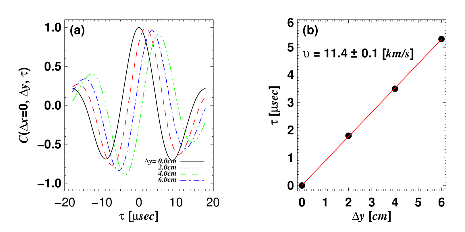
This example is based on a synthetic data set consisting of Gaussian-shaped random “eddies” moving with the poloidal velocity of , which are then used to produce artificial 2D BES data (see Appendix A for the description of the synthetic data). With the four available poloidal channels, cross-correlation functions are calculated using equation (2) and shown in Figure 1(a); is plotted as a function of in Figure 1(b). The inverse of the slope of a fitted straight line is the velocity . Note the slight discrepancy between the actual and CCTD-determined velocities. The origin and size of this discrepancy are discussed in Appendix B.
2.2.2 Physical meaning of the velocity determined by the CCTD method
Using the described CCTD method, the 2D BES system on MAST is expected to be able to determine as has been done previously on TFTR [17] and DIII-D [29] using their BES systems [30, 31]. However, as McKee et al. [32, 33] pointed out, one must distinguish between the poloidal velocity measured by 2D BES system () and the actual velocity of the poloidal plasma flow ().
The mean plasma flow can be decomposed into toroidal () and poloidal () components. For typical tokamak plasmas where strong neutral beams are injected, is satisfied as any mean poloidal flows are strongly damped [34, 35], leaving of the order of the diamagnetic velocity , where , is the tokamak minor radius, and is the ion thermal velocity. Note that can be on the order of for the neutral-beam-heated plasmas. Thus, can be ignored compared to , except possibly in regions with strong pressure gradients.
As the 2D BES system on MAST observes the density patterns advected by , there will be an apparent motion of the patterns in the poloidal direction, as shown in Figure 2.
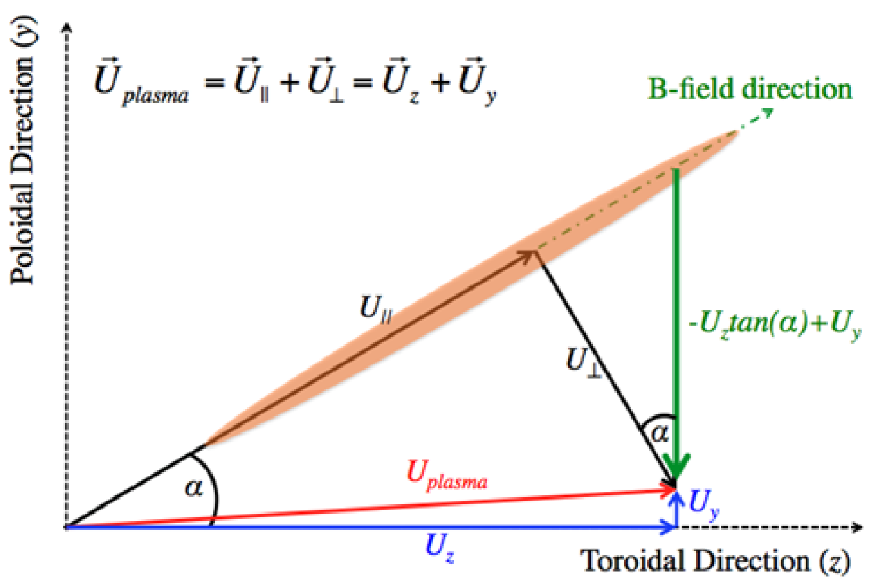
This effect is analogous to the apparent up-down motion of helical strips of a ‘rotating barber-pole’ (cf. [36]). The magnitude of this apparent velocity can be readily calculated via elementary geometry: namely, we expect the BES system to “see”, to lowest order in ,
| (3) |
where is the pitch angle of the local magnetic field line.
Equation (3) is experimentally verifiable because all three physical quantities are readily obtained by separate diagnostics: from the 2D BES system, from the charge exchange recombination spectroscopy (CXRS) system [37], and either from EFIT equilibrium reconstruction [38] or directly from the Motional Stark Effect (MSE) system [39, 40] on MAST. Although the CXRS system measures the toroidal flow of the ions, the difference between the velocity of the ions and the bulk plasma ions, , is predicted to be on the order of in a strongly beam-heated plasma [41]. In section 3, equation (3) will be experimentally verified for various types of discharges. Agreement will indicate consistency of the experiment with the assumptions behind equation (3). Such agreement will indeed be obtained, except in one intriguing case.
Let us now consider what are the assumptions necessary for equation (3) to hold by analysing how the estimated depends on actual physical quantities associated with plasma flows and fluctuations in a tokamak. The cross-correlation function (2) of the normalized fluctuating photon intensity can, in view of equation (1), be considered proportional to the cross-correlation function of the relative ion density fluctuation (by definition, ). Therefore, the CCTD-determined velocity of the density patterns can be related to the actual physical quantities in a tokamak by invoking the ion continuity equation. Splitting also the ion velocity into mean and fluctuating parts, , , we have
| (4) |
Averaging this equation and subtracting the averaged equation from (4), we obtain
| (5) |
We will now order various terms in this equation in terms of the small parameter .
Assuming that the spatial scale of all mean quantities is while the spatial scale of all fluctuating quantities is , and also , we get
| (6) | |||||
where we have dropped all terms and smaller. The first two terms on the right-hand-side are and the following three terms are . Note that we have not yet made any assumptions about the nature of the mean flow (beyond it being large-scale) or about time scale of the fluctuations.
In fact, the ordering, which is the standard gyrokinetic ordering [42], can take us further: it is possible to show that compressibility effects are order , i.e., , and that the mean flow to lowest order is purely toroidal [34, 35]: , where is the toroidal direction (locally) and including all poloidal flows†††Note that the poloidal velocity of the bulk plasma ions has been measured with the CXRS system to be only a few on MAST [43], which is consistent with . Such measurements are, however, not routinely available for MAST, and one of the goals for this study is to confirm that is indeed small. and first-order corrections to (radial flows, associated with particle fluxes, are, in fact, even smaller). Coupled with the fact that mean quantities have no toroidal variation in a tokamak, this means that that the fifth term on the right-hand-side of equation (6) is also , while the first term can be expressed as
| (7) | |||||
where is the unit vector in the direction of the magnetic field in a local orthogonal Cartesian system (: radial, : poloidal and : toroidal), and we have used the identity . Making a further assumption, again standard in gyrokinetics, that the parallel spatial scale of the fluctuating quantities is , we conclude that the second term in the second line of equation (7) is .
Finally, combining equation (7) with (6), we find
| (8) |
where is the dominant apparent velocity of the density patterns ( is the local pitch angle of the magnetic field line). The term containing is the only term in equation (8). The and higher terms have been assembled in the right-hand-side: by definition, is such that
| (9) | |||||
This contains, in order of terms, the effects associated with
(1) parallel variations of the fluctuations,
(2) mean poloidal flows of bulk plasma ions,
(3) compressibility of the fluctuations,
(4) linear response to mean density gradient (drift waves),
(5) nonlinear effects (turbulence),
and a slew of higher-order effects of varying degree of obscurity.
Thus, the right-hand-side of equation (8) contains all the nontrivial physics of waves and turbulence in the plasma. The apparent velocity of the density patterns detected by the 2D BES system will not be influenced by these effects to dominant order — if the orderings assumed above are correct. What it does contain is the poloidal signature of the dominant toroidal rotation of the plasma — the ‘rotating barber-pole’ effect discussed at the beginning of this section. Indeed, if equation (8) holds and its right-hand-side is small, then, to lowest order, the density patterns just drift in the -direction (poloidal) with the velocity , so the maximum of the cross-correlation function (2) will be achieved at . Hence equation (3) for the BES-measured velocity.
If we are able to confirm equation (3) experimentally, this means that the theoretical considerations employed above are consistent with the experiment. This is important because most of the theories of tokamak turbulence rely on such considerations. Note that there are no separate diagnostics capable of measuring individually all the terms in equation (9). Therefore, the only conclusion one can formally draw from equation (3) holding is that the sum of these terms is small.
3 Experimental results
In this section, we apply the CCTD method to 2D BES data from MAST discharges to determine the apparent mean poloidal motion () of the ion density patterns. Then, is compared with the ‘rotating barber-pole’ velocity () where the toroidal plasma velocity is obtained from the CXRS system [37] and the local magnetic pitch angle either from EFIT equilibrium reconstruction [38] or the MSE system [39, 40].
The 2D BES data are first bandpass-filtered from to to reduce the noise level. The low-pass filter removes the high-frequency noise component from the photon shot noise and electronic noise, while the high-pass filter reduces the contribution to the signal from low-frequency, coherent MHD (magnetohydrodynamic) modes. The apparent mean poloidal velocity of the density patterns is determined from average correlation functions calculated over time intervals of duration, resulting in total averaging. Second-order polynomial fitting is applied to interpolate the correlation function on times shorter than the sampling time of as described in Appendix B.1. Finally, five consecutive values of obtained in this manner are averaged, so the total averaging time is which is the effective time resolution of . Using these five values of , the time average of various errors defined in equations (18)-(20) in Appendix B.2 are also computed. Statistical reliability of the CCTD method is investigated in Appendix B by using the synthetic 2D BES data (Appendix A).
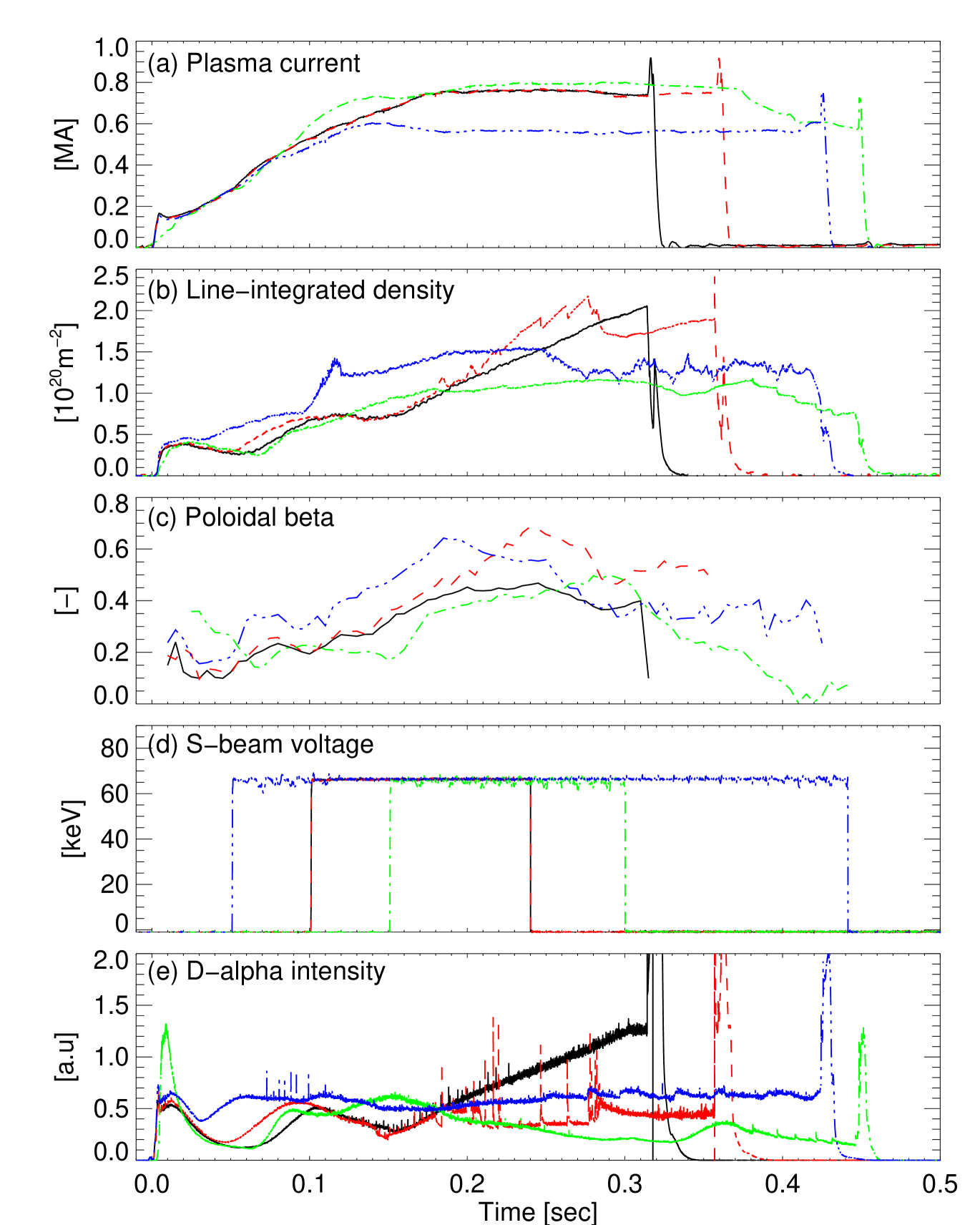
We present measurements of from four different discharges: shot #27278 (L-mode), shot #27276 (H-mode), shot #27269 (ITB) and shot #27385 (high-poloidal-beta). All four discharges had double-null diverted (DND) magnetic configurations and co-current NBI (neutral beam injection). In all of these discharges, the 2D BES system viewed at nominal major radial position of corresponding to normalized minor radii for L- and H-modes, and - for ITB and high-poloidal-beta discharges. The evolution of key parameters for these discharges is shown in Figure 3. The evolution of plasma current, line-integrated electron density and poloidal beta characterize the overall behaviour of plasmas, while the non-zero S-beam voltage corresponds to times when the 2D BES system obtains localized density fluctuation. The intensity trace is used to identify when the H-mode discharge (shot #27276) goes into its H-mode: namely, at . Note that the ITB discharge (shot #27269) starts developing a strong temperature gradient at and the peak ion ( from the CXRS) temperature keeps increasing until the NBI cuts off at . The viewing position of the 2D BES system is in the middle of the strong temperature gradient region for this discharge.
3.1 L-mode (shot #27278), H-mode (shot #27276) and ITB (shot #27269) discharges:
Time evolution of (a) cross-power of the fluctuating magnetic field signal from two toroidally separated outboard Mirnov coils, (b) cross-power and (c) temporal cross-correlation of density fluctuations from two poloidally separated BES channels (two mid-channels separated by ) located at are shown in Figures 4 (L-mode), 5 (H-mode) and 6 (ITB discharge). Here, a cross-power is defined as the Fourier transform (in the time domain) of the cross-correlation function (2) with finite channel separation.
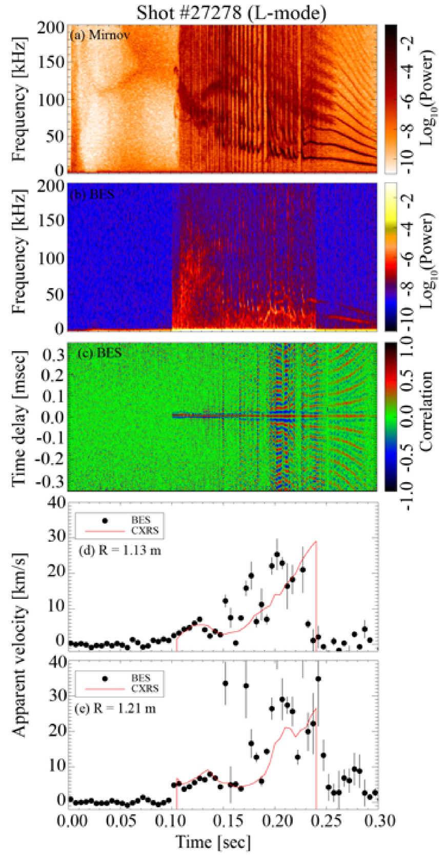
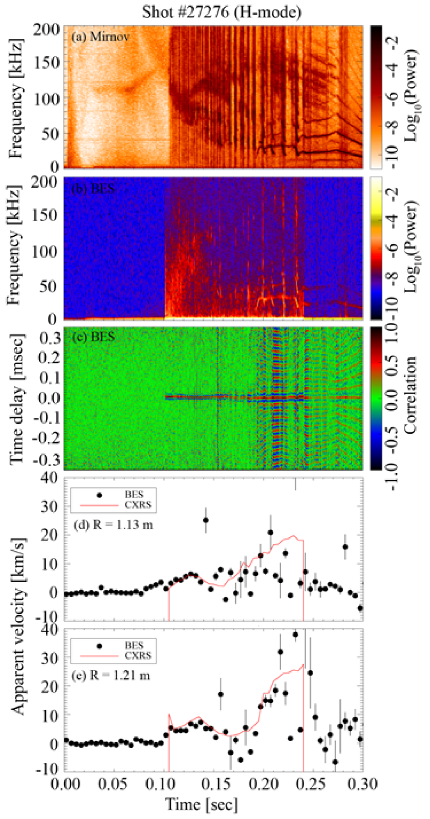
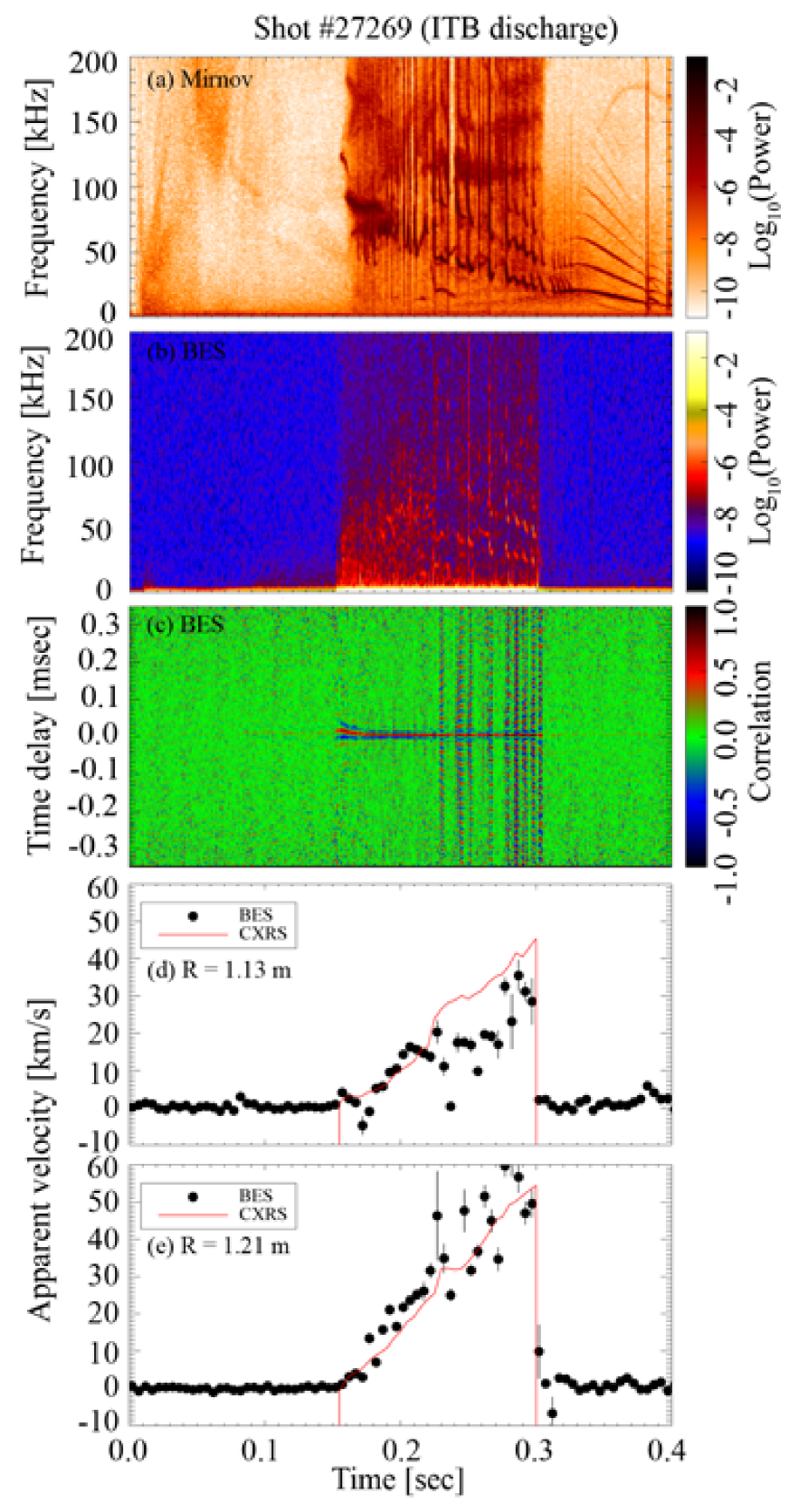
The (minus) apparent mean poloidal velocity (, circles) determined by the CCTD method and the ‘rotating barber-pole’ velocity (, red solid lines) are also shown in panels (d) at and (e) at for these three discharges. The error bars represent the mean error of the least-squares fit, as discusses in Appendix B.2.
Despite the fact that these three discharges belong to three very different classes, there are common features in the apparent mean poloidal velocity:
(1) is not reliable (i.e., has large error bars) when strong MHD activity is present. The cross-power spectrograms from BES show clear signatures of MHD modes with many harmonics, which hamper filtering the BES signal over the frequency domain. The temporal cross-correlations also show that these MHD modes have much longer correlation times () than the turbulent density patterns. The effects of MHD (global) modes on the CCTD method are investigated in Appendix B.5, where it is found that such activity can increase not only the absolute values of the bias errors but also the linear fitting errors on . Thus, comparisons between and are difficult to make during the periods where the MHD activity is strong.
(2) During the periods of weak MHD activity, i.e., - for the L- and H-mode discharges, and - for the ITB discharge, it is clear that the apparent mean poloidal velocity of turbulent density patterns is dominated by the ‘rotating barber-pole’ velocity, i.e., equation (3) holds, and the sum of all the terms of the order of or higher in equation (9) is indeed small.
Note that the H-mode discharge (shot #27276) goes into its H-mode at (thus, is only true before the L-H transition, strictly speaking), which can be seen from the intensity trace in Figure 3 or from the BES cross-power spectrogram in Figure 5: the turbulence level drops at the start of the H-mode. Any changes of during the L-H transition cannot be discussed, because the CCTD method with the current data analysis scheme is not reliable at this time due to strong MHD activity.
3.2 High-poloidal-beta discharge (shot #27385):
Shot #27385 has a relatively higher poloidal beta (the ratio of the plasma pressure to the poloidal magnetic field energy density) than the three discharges discussed in section 3.1 (see Figure 3). Thus, it is more susceptible to tearing modes (i.e., formation of magnetic islands) [44, 45]. The cross-power spectrogram between the two toroidally separated outboard Mirnov coils displayed in Figure 7(a) shows a tearing mode on the =1.5 flux surface starting at ; its frequency increases from to at .
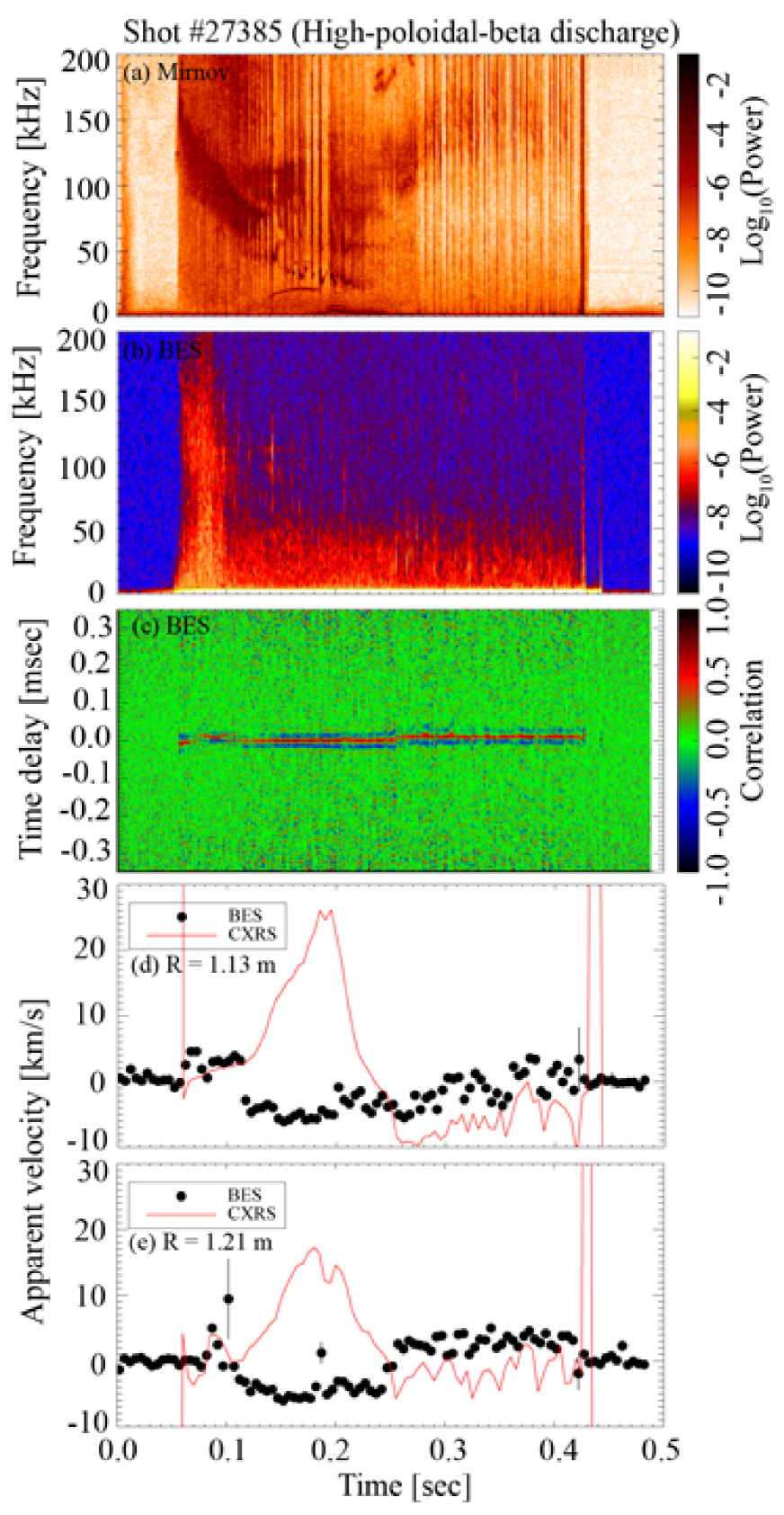
Then, a mode (fundamental frequency ) develops and locks to the wall resulting in complete braking of the toroidal rotation of plasmas at . Here, and denote the poloidal and toroidal mode numbers, respectively, and for the safety factor.
The mode is not expected to be seen on the BES signal as it is bandpass-filtered from , and no trace of the mode is visible in the BES signal‡‡‡Because the mode flattens the mean density profile within the island, shaking of flux surfaces does not induce density fluctuations in the BES signal. Consequently, the determined by the CCTD method does not contain large error bars during the whole discharge.
The time evolution of and in Figure 7(d)-(e) at two different radial locations shows that the two velocities do not agree each other at all during the period when the and modes are present. What we find, remarkably, is that while the plasma continues to rotate toroidally (as attested by the CXRS data), there is virtually no detectable corresponding motion of the density patterns. In fact, they seem to exhibit a weak rotation in the opposite direction to the expected rotating barber-pole effect. Formally, this means that the plasma effects in the right-hand-side of equation (8) are not small and are able to cancel almost exactly the toroidal rotation, i.e., an effective velocity of the density patterns develops in the plasma frame that to lowest order is equal to minus the rotation velocity. We do not currently have a theoretical explanation for this effect. There is very little apparent difference between the turbulent density patterns in this discharge compared to others, except somewhat longer radial correlation lengths.
4 Conclusions
We have analysed 2D BES data from different types of discharges on MAST to determine the apparent mean poloidal velocities of the ion-scale density patterns using the cross-correlation time delay method. The dominant cause of the apparent poloidal motion of the density patterns is experimentally identified to be due to the fact that field aligned patterns are advected by the background, dominantly toroidal, plasma rotational flow, i.e., the ‘rotating barber-pole’ effect dominates the apparent mean motion of the density patterns in the lab frame. This conclusion holds for the L-, H-mode and ITB discharges we have investigated. An exception to this rule is found to be the investigated high-poloidal-beta discharge, where a large magnetic island is present, and the apparent velocity of the density patterns is very small, despite strong toroidal rotation. Identifying the causes of this effect by investigating the behaviour of the turbulent density patterns quantitatively is left for future work.
Acknowledgment
We would like to thank Ian Abel, Steve Cowley, Edmund Highcock, Tim Horbury, Darren McDonald, Clive Michael and Jack Snape for valuable discussions, and Rob Akers for setting up the environment for CUDA programming. This work was funded jointly by the RCUK Energy Programme, by the European Communities under the contract of Association between EURATOM and CCFE and by the Leverhulme Trust International Network for Magnetised Plasma Turbulence. The views and opinions expressed herein do not necessarily reflect those of the European Commission.
Appendix Appendix A Synthetic 2D BES data
Appendix A.1 Gaussian eddies in space and time
It is necessary to know the true mean velocity of the density patterns to investigate statistical reliability of the cross-correlation time delay (CCTD) method described in section 2.2. Specifically, we investigate how reliable the CCTD method is for different magnitudes of mean velocities and correlation times of the density patterns. We must also evaluate the effect of global modes (i.e., MHD modes) and temporally varying poloidal velocities on the CCTD method. For this purpose, we numerically generate artificial density patterns, random both in space and time, then produce synthetic BES data using the point-spread-functions (PSFs) of the 2D BES system on MAST (as described in Appendix A.2) and compare the inferred flow velocity with the true flow velocity.
We follow a similar approach to the one suggested by Zoletnik et al. [46]. Let the density patterns be described by Gaussian structures both in space and time, namely,
| (10) | |||||
where , and denote radial, poloidal and time coordinates, respectively. These numerically generated density patterns are referred to as “eddies” in this paper. Here is the total number of eddies and the subscript denotes the eddy in the simulation; , , and are the maximum amplitude and central locations in the , and coordinates of the eddy, respectively; , and are the widths of our Gaussian eddies in the , and directions; is the lifetime (or the correlation time) of the eddies in the moving frame; is the apparent advection velocity of the eddies in the poloidal direction. Although it is possible to introduce a finite radial velocity shear by making a function of , the effect of such shearing rates on the CCTD method is not investigated in this paper, so we will only consider that are independent of . The term in the (poloidal) direction is introduced to model wave-like-structured eddies in the poloidal direction as observed in tokamaks [47]. Note that the envelope (i.e., the term) and the wave structure (i.e., the term) of have the same advection velocity . The central locations of eddies, , and , are selected from uniformly distributed random numbers, whereas their amplitudes are selected from normally distributed random numbers whose standard deviation is one.§§§It is worth mentioning that there is another scheme of generating such eddies numerically, proposed by Jakubowski et al. [48]. They generated the time series of fluctuating density () using the inverse Fourier transform of a broadband Gaussian amplitude distribution in frequency space. Then, a second signal () was generated by imposing the desired time-delay fluctuation on the such that was a time-delayed version of . This method does not include spatial information for the signals.
The spatial domain of the simulation is and with the mesh size of in radial () and poloidal () directions, respectively. The time duration of the simulation is with a time step so as to have the same Nyquist frequency as the real 2D BES data from MAST. The widths and are set so that the full width at half maximum (FWHM) in the radial direction and the wavelength in the poloidal direction are (i.e., ) and (i.e., ), respectively, which are similar to the measured correlation lengths with the 2D BES system on MAST.¶¶¶Note that Smith et al. [49] also reported that poloidal correlation lengths of the density patterns are using their 2D BES system on NSTX. The eddy lifetime in the moving frame () is set to . However, some of the data sets in this paper have different values of , so the effect of on the CCTD method can be investigated.
The total number of eddies is . If the eddies are too sparse in the simulation domain, then we may not achieve steady statistical results, while overly dense eddies may cause an effective widening of the specified spatial ( and ) and temporal () correlations as many eddies can merge into one larger eddy. Thus, we introduce another control parameter, the spatio-temporal filling factor (), defined as
| (11) |
where is the autocorrelation time calculated as
| (12) |
for the generated eddies defined by equation (10). All of our synthetic data was generated so as to .
The testing of the CCTD method will involve exploiting what happens if has a mean and a temporally varying components. Thus, we generate a temporal structure of : at each ,
| (13) | |||||
where and are the mean and temporally varying velocities, respectively, and are the lifetime and frequency of , respectively, and is generated from normally distributed random numbers. The RMS (root-mean-square) value of denoted as will be varied as well as to investigate the effects of these quantities on the CCTD method. and allow one to introduce structured temporally varying velocities, while the randomness is kept by . As one of the causes for the temporal variation of the poloidal velocity is believed to be the existence of geodesic acoustic modes (GAMs)∥∥∥We do not investigate whether the CCTD method is able to detect such a temporally structured (or GAMs) in this paper, rather we investigate how the existence of these structures affects the CCTD-determined mean velocity. [50], we choose and to mimic the GAM features detected by Langmuir probes on MAST [51].
The simulations have been run on a NVIDIA® GeForce GTS 250 GPU card using CUDA programming, which increases the computational speed owing to the highly parallelizable structure of equation (10).
Appendix A.2 Synthetic 2D BES data
We generate the (1 to 8) radial and (1 to 4) poloidal channel of the synthetic BES data by using the calculated point-spread-functions (PSFs) of the actual 2D BES system on MAST [23] and from equation (10) with an additional random noise. Furthermore, a large-scale (in space) coherent (in time) oscillation is included to imitate a global MHD mode. Namely, is defined as
| (14) |
where is the DC value – a typical value of is used for all channels [16]. The rest of the terms are as follows.
is the fluctuating part of the signal generated from the Gaussian eddies, , given by equation (10) and convolved with the PSFs of the 2D BES system :
| (15) |
where is the PSF of the and channel of the 2D BES system, normalized so that RMS value of is . This value is set so that the ratio of to is 0.05. An example of the PSFs for the 32 channels of the 2D BES system on MAST is shown in Figure 9 (white contour lines in the top-left panel).
models an MHD (global) mode. We assume that the spatial scale of the MHD modes is larger than the BES domain in the poloidal direction, so does not vary in the poloidal direction. The model MHD signal is generated in a way similar to temporal behaviour of using equation (13), except that the mean value of is zero and . The frequency of the mode and its RMS value, denoted , will be varied in various tests. The value of here is representative of MHD burst-like fishbone instabilities [52] or chirping modes [53] in tokamaks, for which the spectrum has a finite bandwidth.
represents the noise in the signal. As the noise of the 2D BES system on MAST is dominated by the photon noise [19], is generated using normally distributed random numbers. Its RMS level is set such that the signal-to-noise ratio () is , which is typical of the 2D BES system on MAST [16].
Figure 8 shows examples of autopower spectra of the synthetic 2D BES data for and . The autopower spectrum is calculated as where is the Fourier transform in the time domain.
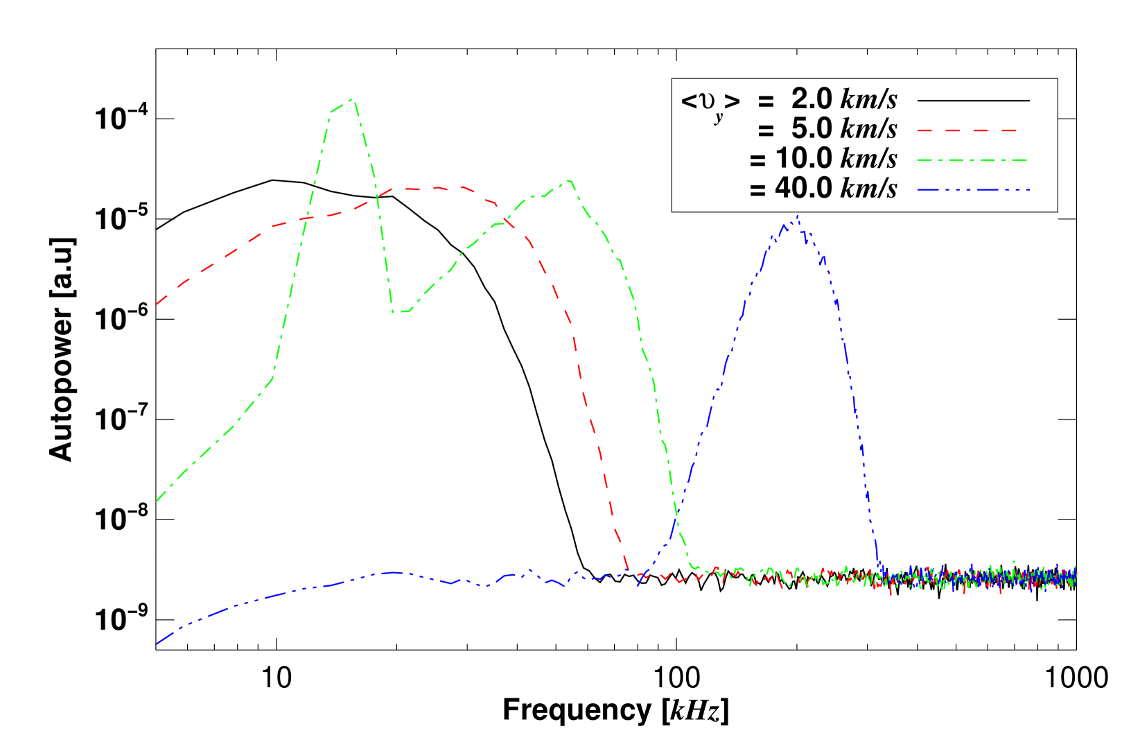
Increasing the value of has two effects: Doppler shift and broadening of the spectra, as expected. Note that in Figure 8, the data for contains the finite with and , while for other cases.
Figure 9 shows several time snapshots of artificial Gaussian eddies (equation (10)) in the left column and the corresponding synthetic 2D BES data in the right column (with DC component removed from equation (14)).
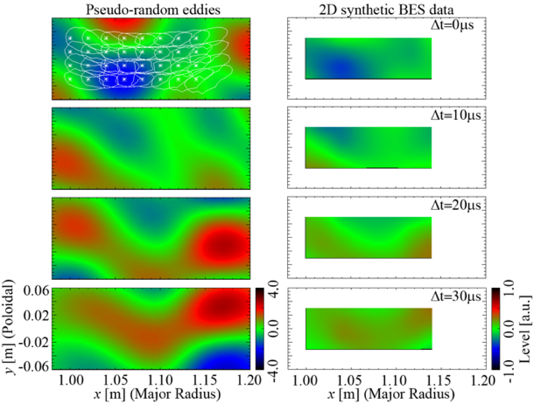
The eddies are moving upward with . The top left panel in this figure also shows the contour lines of the PSFs for the 32 channels [23]. Snapshots for the synthetic 2D BES data are generated with the bandpass frequency filtering from to to suppress the noise. As the synthetic 2D BES data have only 32 spatial points, spatial interpolation is performed using parametric cubic convolution technique [54].
Appendix Appendix B Assessment of the CCTD method
In this section, errors involved in determining the mean velocity of the density patterns by the CCTD method are examined using the synthetic 2D BES data generated according to the procedure explained in Appendix A. The velocity measured via the correlation function (equation (2)) is denoted and compared with the prescribed value that appears in equation (13), i.e., the mean poloidal velocity of the synthetic data. Appendix B.1 provides detailed description of the CCTD method used in this paper, then four types of error are identified for the quantitative comparisons. These errors are evaluated in Appendix B.3 and Appendix B.4 for different values of and the eddy correlation time . Subsequent sections are devoted to investigating how the existence of global (MHD) modes and temporally varying poloidal velocity affect the errors.
Appendix B.1 Description of the CCTD method
As defined by equation (2), cross-correlation functions are calculated as time averages of the data. For a -long synthetic data set containing data points with the sampling time , we want to determine with a time resolution . First, a cross-correlation function (2) is calculated on a sub-time window of the synthetic 2D BES data containing points, where . Then, such cross-correlation functions are averaged over consecutive sub-time windows where so that an averaged cross-correlation function is obtained at every . In this paper, we use , so .
Denoting and the time series over a sub-time window from two poloidally separated synthetic 2D BES channels, the cross-correlation function (2) for this sub-time window is:
| (16) |
for any integer with . Finally, by averaging for consecutive sub-time windows we obtain the smoothed averaged cross-correlation function from -long data points.
The CCTD method has a serious limitation due to the fact that the sampling time is finite. In order to calculate using only two poloidally separated channels, a line is fitted through two points on a plane as shown in Figure 1(b). The first point is located at by definition, and the second point at . Then, possible values of are restricted to where is an integer. For the 2D BES system on MAST, using two adjacent poloidal channels () with a sampling time , the possible values of are limited to for . Such a limitation may be mitigated by using four poloidally separated channels. However, using four channels is not always possible if the channels that are farthest apart are not correlated. To resolve this issue, we use a second-order polynomial fit on the cross-correlation function to locate its global maximum: if is the point where the discrete cross-correlation function is maximum, we use the three values of at , and to fit a second-order polynomial. The “true” maximum is found from this fit. We denote the time delay at which this maximum is reached by .
Appendix B.2 Definition of errors
For a given set of -long synthetic 2D BES data, we calculate with the time resolution of (Appendix B.1). Furthermore, we do this at three different radial locations******As described in Appendix A, are identical at all radial locations. One column in the middle and two columns from the edges of the 2D BES channels are used. so that the average of , denoted , can be calculated using values of . To make quantitative comparisons between and defined in equation (13), we define four types of error.
The normalized bias error
| (17) |
is a quantitative measurement of the systematic discrepancy between the measured and the true value. The normalized random error
| (18) |
quantifies the degree of fluctuation in the measured with respect to . This value may depend on the MHD contribution in equation (14) and the temporally varying poloidal velocity in equation (13).
Furthermore, as linear fitting is done to determine (see Figure 1), two other types of error are present. The slope of a linear fit can be denoted as where is a degree of the uncertainty of the least-square fit††††††In Figure 1, we plotted as a function of and determined as the inverse of the slope of a fitted line. Operationally, we actually plot as a function of so the slope of a fitted line is the .. Then, the normalized mean of is
| (19) |
and the normalized random error in is
| (20) |
These two uncertainties together provide an estimation of how well a linear line is fitted to given data points. For example, if the assumption that is long enough so that all four poloidally separated channels observe the same eddies is not satisfied, then becomes large. On the other hand, if this assumption is occasionally satisfied, then exhibits such events because will then be small compared to its average. Note that error bars of the CCTD-determined apparent velocities in Figures 4 - 7 show .
In the following sections, these four types of error will be evaluated for various values of and , and various ranges of , and .
Appendix B.3 Measuring mean velocity
To investigate the reliability of the CCTD method described in Appendix B.1 for estimating , we generate a number of synthetic 2D BES data sets with various values of while keeping all the other parameters in equations (10), (13), (14) and (15) constant. In real experiments, there is almost always some temporal variation of , thus the RMS value of in equation (13) is set to of in this subsection. The synthetic 2D BES data are frequency-filtered to suppress the noise before the cross-correlation functions are calculated. Figure 10 shows examples of (a) generated according to equation (13) with and (b) the original (black) and frequency-filtered (red) autopower spectra of a generated synthetic signal. Here, the noise cut-off level is set to be the times the averaged autopower level above (green dashed line).
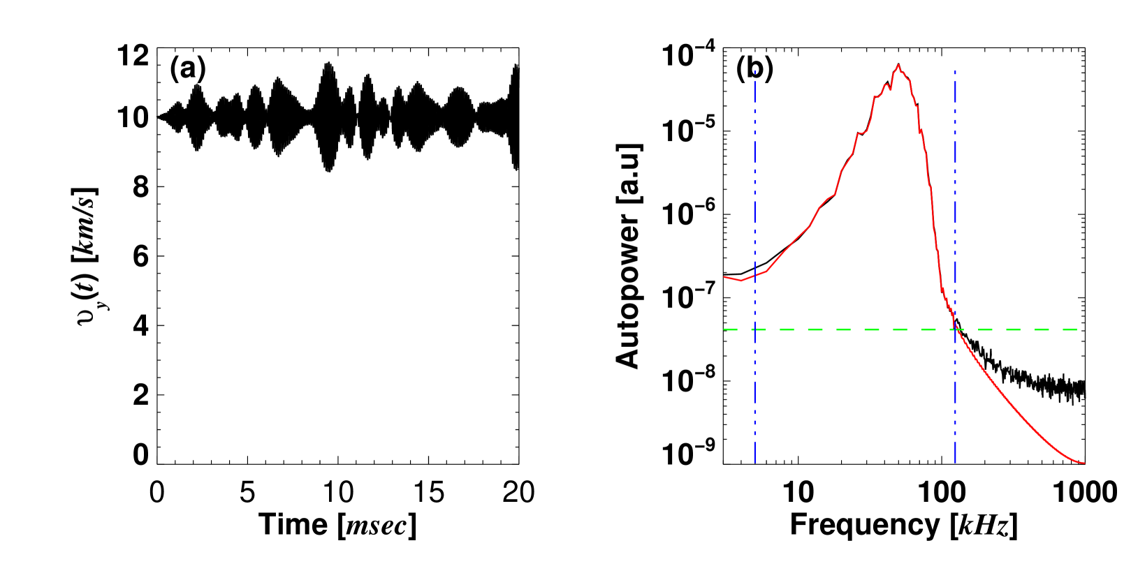
Figure 11 shows , , and defined in Appendix B.2 and calculated for values of ranging from to . The basic conclusions that can be made based on these results are as follows:
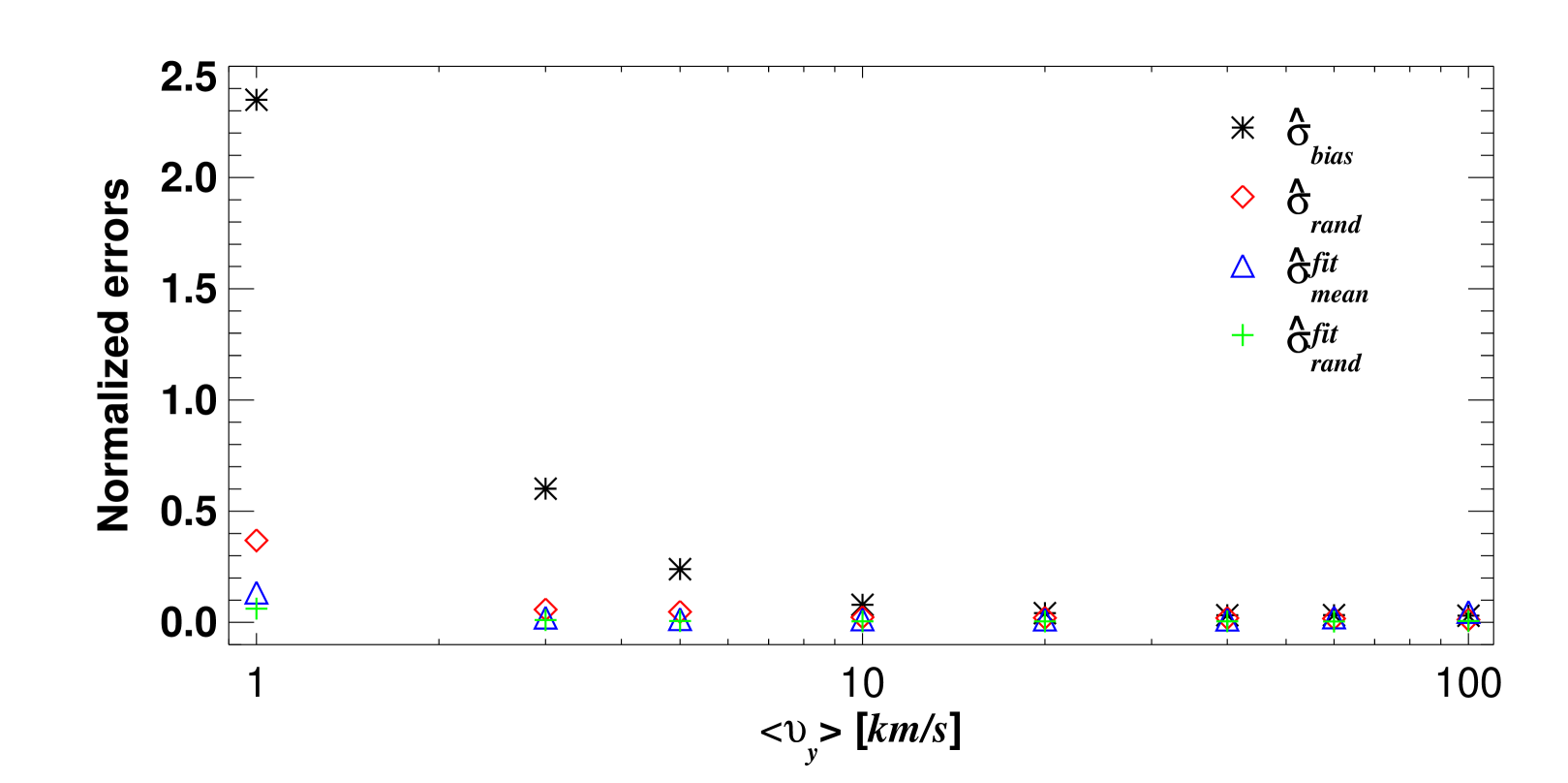
(1) For , the CCTD method is not reliable. This is due to the fact that eddies do not live long enough to be detected by all the poloidally separated channels. Indeed, it was a priori clear that could not be measured. This translates to for and , so our results are consistent with this simple criterion.
(2) The CCTD method usually overestimates (i.e., ). This can be explained by the effective channel separation distance () being in fact slightly less than because of the overlapping of the PSFs, as shown in Figure 9.
(3) The limitation of the CCTD method due to the finite is successfully overcome by fitting a second order polynomial to the cross-correlation function, as explained in Appendix B.1.
Appendix B.4 Effect of the eddy lifetime
As explained in section 2.2.2, the CCTD method for determining is based on the idea that the peak of the cross-correlation function occurs at , where is the propagation time of the fluctuating density patterns between detectors poloidally separated by the distance . However, will not coincide with if the lifetime of the fluctuations is not long compared to . The failure of the method for illustrated in Figure 11 is an example of what happens when is too large. Here, we investigate the effect of on quantitatively, via a systematic scan of the synthetic BES data.
Two values and are chosen for this study. For , , and with , and , respectively; for , they are , and . The peak time is found using the polynomial fitting method described in Appendix B.1, and as a function of is plotted for three different values of in Figure 12. It shows that underestimates the true for small values of , leading to an overestimation of the , consistent with the results shown in Figure 11. It is encouraging, however, that even relatively low velocities of just a few can be determined by the CCTD method with reasonable accuracy ().
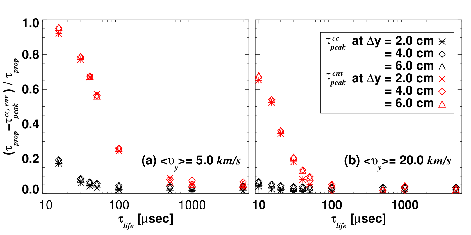
It is also possible to consider the global maximum of the envelope of the cross-correlation function. We use Hilbert transform to determine the time delay at which the envelope of the cross-correlation function is maximum [17]. The comparison between and is shown in Figure 12. It is clear that has a much stronger dependence on than , so this measure will not be used to estimate in this paper. We note, however, that the strong dependence of on the eddies’ lifetime and of on their propagation time may provide a way to measure correlation times in the plasma frame. Such an investigation is currently being pursued and will be reported elsewhere.
Appendix B.5 Effect of coherent MHD modes
Many experimental 2D BES data sets on MAST exhibit strong MHD (global mode) activity in addition to the small-scale turbulence. Removing such global modes in the frequency domain is not straightforward as they can have multiple harmonics extending into higher frequencies. While they could be filtered out relatively easily in the wavenumber domain, constructing wavenumber spectra with a very limited number of spatial data points is difficult. Thus, it is useful to investigate how the presence of such modes affects the quality of our measurement of . In this section, this is done by using synthetic BES data sets with different RMS levels and frequencies of the global oscillations (the term in equation (14)).
The four errors (, , and ) are calculated for various ratio of to the RMS value of (i.e., in equation (15)). These errors are plotted in Figure 13(a) for the scan.
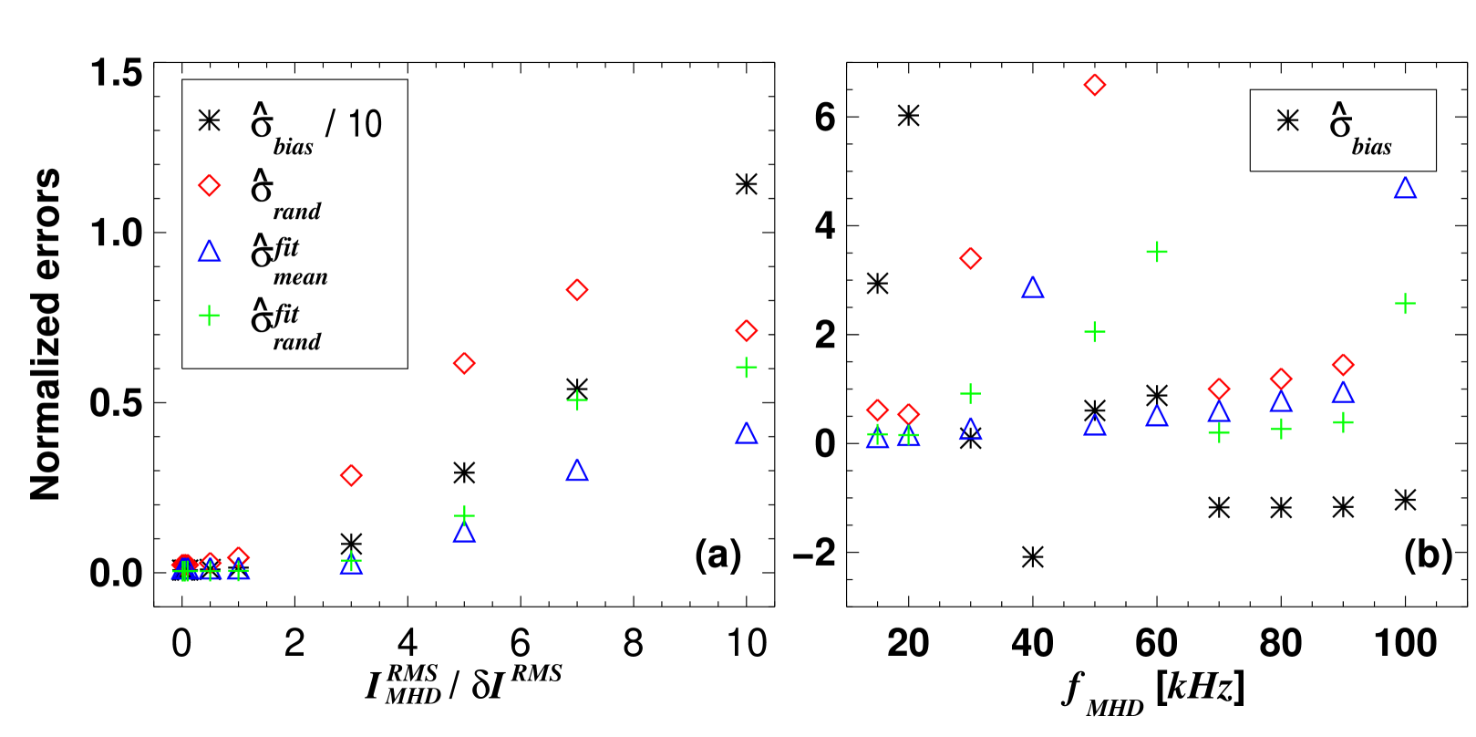
Here, the frequency of the global mode and . It is clear that if the power level of the mode is larger than that of the turbulence signal, then the CCTD method produces large bias errors . To examine how the frequency of a global mode affects the errors, is varied with a fixed value of . The results of this scan are shown in Figure 13(b). It shows that can be either positive or negative with different values of meaning that global modes in real experimental data can cause both over- and under-estimation of the true .
Figure 14 shows how different frequencies can cause such an over- or under-estimation of the .
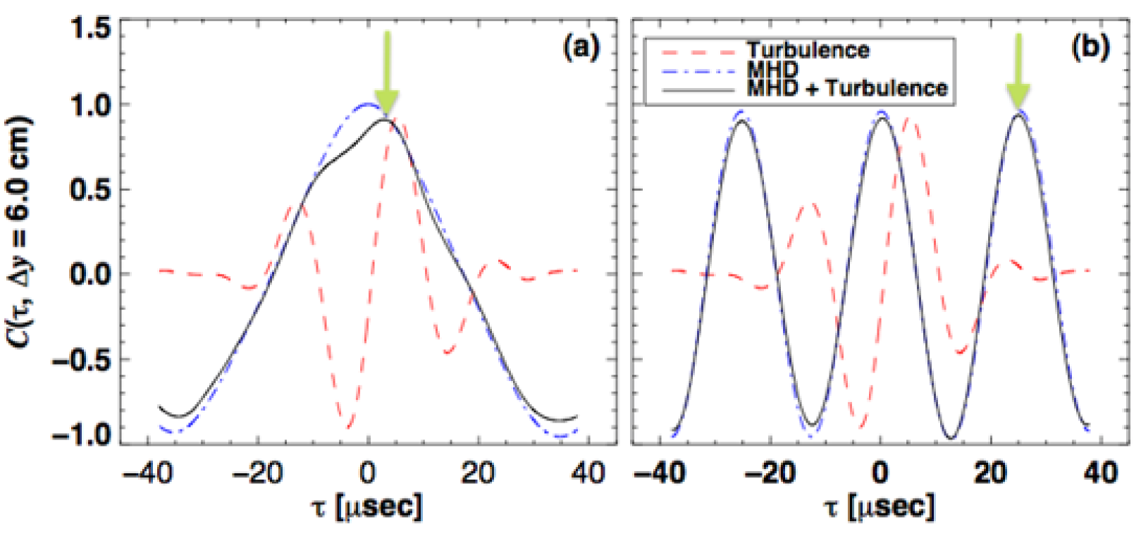
Two identical sets of synthetic BES data with are generated, one with and another without a global mode at (a) and (b) , with . Without the global modes, the cross-correlation functions with (red dashes in Figure 14) have the expected value for both cases. In contrast, the presence of the global mode in the synthetic BES data shifts towards (a) smaller time-lag (over-estimation) or (b) larger time-lag (under-estimation).
We conclude that a global (MHD) mode with affects the structure of the cross-correlation functions (both the shape and the position of ) rendering the CCTD method unreliable.
Appendix B.6 Effect of temporally varying poloidal velocity
No physical quantities are absolutely quiet in real experiments, thus it is necessary to investigate how the RMS level of the temporal variation of the poloidal velocity (see equation (13)) influences the measurement of .
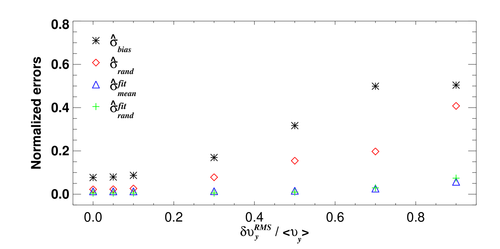
Figure 15 shows how finite (with ) affect the four errors defined in Appendix B.2. It appears that saturates at around for the scenarios we have investigated, while other three errors increase without showing any sign of saturation. Thus, the CCTD method to measure is subject to a non-negligible bias error (up to ) if the RMS level of temporal variation of the poloidal velocity is greater than a half of the mean poloidal velocity.
References
- [1] Carreras B A 1997 IEEE Trans. Plasma Sci. 25 1281
- [2] Highcock E G, Barnes M, Parra F I, Schekochihin A A, Roach C M and Cowley S C 2011 Phys. Plasmas 18 102304
- [3] Highcock E G, Barnes M, Schekochihin A A, Parra F I, Roach C M and Cowley S C 2010 Phys. Rev. Lett. 105 215003
- [4] Waltz R, Kerbel G and Milovich J 1994 Phys. Plasmas 1 2299
- [5] Waltz R, Staebler G, Dorland W, Hammett G, Kotschenreuther M and Konings J 1997 Phys. Plasmas 4 2482
- [6] Dimits A, Cohen B, Nevins W and Shumaker D 2001 Nucl. Fusion 41 1725
- [7] Kinsey J E, Waltz R E and Candy J 2005 Phys. Plasmas 12 062302
- [8] Camenen Y, Peeters A, Angioni C, Casson F, Hornsby W, Snodin A and Strintzi D 2009 Phys. Plasmas 16 012503
- [9] Roach C et al. 2009 Plasma Phys. Control. Fusion 51 124020
- [10] Barnes M, Parra F, Highcock E, Schekochihin, Cowley S and Roach C 2011 Phys. Rev. Lett. 106 175004
- [11] Burrell K 1997 Phys. Plasmas 4 1499
- [12] Connor J W, Fukuda T, Garbet X, Gormezano C, Mukhovatov V, Wakatani M, the ITB Database Group and the ITPA Topical Group on Transport and internal Barrier Physics 2004 Nucl. Fusion 44 R1
- [13] Mantica P et al. 2009 Phys. Rev. Lett. 102 175002
- [14] Mantica P et al. 2011 Phys. Rev. Lett. 107 135004
- [15] de Vries P C et al. 2009 Nucl. Fusion 49 075007
- [16] Field A R, Dunai D, Gaffka R, Ghim Y-c, Kiss I, Mészáros B, Krizsanóczi T, Shibaev S, Zoletnik S 2011 Rev. Sci. Instrum. 83 013508
- [17] Durst D, Fonck R J, Cosby G and Evensen H 1992 Rev. Sci. Instrum. 63 4907
- [18] Cosby G 1992 Master’s Thesis, Department of Nuclear Engineering and Engineering Physics, University of Wisconsin - Madison, WI, USA
- [19] Dunai D, Zoletnik S, Sárközi J and Field A R 2010 Rev. Sci. Instrum. 81 103503
- [20] Field A R, Dunai D, Conway N J, Zoletnik S and Sárközi J 2009 Rev. Sci. Instrum. 80 073503
- [21] Fonck R J, Duperrex P A and Paul S F 1990 Rev. Sci. Instrum. 61 3487
- [22] Summer H P 2004 The ADAS User Manual, ver. 2.8, http://adas.phys.strath.ac.uk
- [23] Ghim Y-c, Field A R, Zoletnik S and Dunai D 2010 Rev. Sci. Instrum. 81 10D713
- [24] Shafer M. W., Fonck R. J., McKee G. R., Holland C., White A. E. and Schlossberg D. J. 2012 Phys. Plasmas 19 032504
- [25] Zweben S J, Terry J L, Agostini M, Hager R, Hughes J W, Myra J R, Pace D C and the Alcator C-Mod Group 2012 Plasma Phys. Control. Fusion 54 025008
- [26] Tal B, Bencze A, Zoletnik S, Veres G and Por G 2011 Phys. Plasmas 18 122304
- [27] Xu Y et al 2011 Plasma Phys. Control. Fusion 53 095015
- [28] Zweben S J et al 2006 Phys. Plasmas 13 056114
- [29] Jakubowski M, Fonck R J and McKee G R 2002 Phys. Rev. Lett. 89 265003
- [30] Paul F and Fonck R J 1990 Rev. Sci. Instrum. 61 3496
- [31] McKee G, Ashley R, Durst R, Fonck R, Jakubowski M, Tritz K, Burrell K, Greenfield C and Robinson J 1999 Rev. Sci. Instrum. 70 913
- [32] McKee G R et al 2003 Phys. Plasmas 10 1712
- [33] McKee G R, Fenzi C, Fonck R J and Jakubowski M 2003 Rev. Sci. Instrum. 74 2014
- [34] Hirshman S P and Sigmar D J 1981 Nucl. Fusion 21 1079
- [35] Helander P and Sigmar D J 2002 Collisional Transport in Magnetized Plasmas (Cambridge University Press)
- [36] Munsat T and Zweben S J 2006 Rev. Sci. Instrum. 77 103501
- [37] Conway N J, Carolan P G, McCone J, Walsh M J and Wisse M 2006 Rev. Sci. Instrum. 77 10F131
- [38] Lao L L, St John H, Stambaugh R D, Kellman A G and Pfeiffer W 1985 Nucl. Fusion 25 1611
- [39] Kuldkepp M, Walsh M J, Carolan P G, Conway N J, Hawkes N C, McCone J, Rachlew E and Wearing G 2006 Rev. Sci. Instrum. 77 10E905
- [40] De Bock M F M, Conway N J, Walsh M J, Carolan P G and Hawkes N C 2008 Rev. Sci. Instrum. 79 10F524
- [41] Kim Y B, Diamond P H and Groebner R J 1991 Phys. Fluids B 3 2050
- [42] Frieman E A and Chen L 1982 Phys. Fluids 25 502
- [43] Field A R, McCone J, Conway N J, Dunstan M, Newton S and Wisse M 2009 Plasma Phys. Control. Fusion 51 105002
- [44] La Haye R J, Buttery R J, Guenter S, Huysmans G T A, Maraschek M and Wilson H R 2000 Phys. Plasmas 7 3349
- [45] Buttery R J, Sauter O, Akers R, Gryaznevich M, Martin R, Warrick C D, Wilson H R and the MAST Team 2002 Phys. Rev. Lett. 88 125005
- [46] Zoletnik S, Petravich G, Bencze A, Berta M, Fiedler S, McCormick K and Schweinzer J 2005 Rev. Sci. Instrum. 76 073504
- [47] Fonck R J, Cosby G, Durst R D, Paul S F, Bretz N, Scott S, Synakowski E and Taylor G 1993 Phys. Rev. Lett. 70 3736
- [48] Jakubowski M, Fonck R J, Fenzi C and McKee G R 2001 Rev. Sci. Instrum. 72 996
- [49] Smith D R, Fonck R J, McKee G R, Thompson D S and Uzun-Kaymak I U 2011 53rd DPP Meeting of the APS
- [50] Winsor N, Johnson J L and Dawson J M 1968 Phys. Fluids 11 2448
- [51] Robinson J R, Hnat B, Dura, P, Kirk A, Tamain P and the MAST Team Phys. Rev. Lett. submitted
- [52] McGuire K et al 1983 Phys. Rev. Lett. 50 891
- [53] Gryaznevich M P and Sharapov S E 2004 Plasma Phys. Control. Fusion 46 S15
- [54] Park S K and Schowengerdt R A 1982 Computer vision, graphics, and image processing 23 258