Measurement of the cross section from threshold to 3.00 GeV using events with initial-state radiation
Using initial-state radiation events from a total integrated luminosity of 11.957 fb-1 of collision data collected at center-of-mass energies between 3.773 and 4.258 GeV with the BESIII detector at BEPCII, the cross section for the process is measured in 16 invariant mass intervals from the production threshold up to 3.00 GeV. The results are consistent with previous results from BaBar and BESIII, but with better precision and with narrower invariant mass intervals than BaBar.
I INTRODUCTION
Electromagnetic form factors (EMFFs), which parametrize the inner structure of hadrons, are fundamental observables for understanding the strong interaction. In the timelike region, EMFFs are extensively studied in electron-positron collisions by measuring hadron pair production cross sections. For a spin- baryon (), the cross section in the Born approximation of the one-photon-exchange process is parameterized in terms of electric and magnetic form factors and by Cabibbo and Gatto (1961):
| (1) |
where is the fine-structure constant, is the Coulomb correction factor Brodsky and Lebed (2009), is a phase-space (PHSP) factor, is the square of the center-of-mass (c.m.) energy, is the mass of the baryon, and is the speed of light. accounts for the electromagnetic interaction of the fermions in the final state, and in the point-like approximation, it is 1 for neutral baryons and with for charged baryons. Therefore, for charged baryon-pairs, the factor of due to PHSP is canceled by the Coulomb factor, which results in a non-zero cross section at the threshold when . However, there is no cancelation in the neutral baryon-pair case, so the cross section is zero.
There have been many experimental studies on the charged and neutral baryon-pair production cross sections in the past decades, such as Ablikim et al. (2020a); Lees et al. (2013), Ablikim et al. (2021a), Aubert et al. (2007); Ablikim et al. (2018a, 2019a); Bisello et al. (1990), Ablikim et al. (2021b, 2022a), Ablikim et al. (2021c, d), and Ablikim et al. (2018b). Although the conclusions for some channels are questionable due to large uncertainties, there is a general tendency in the production cross sections for these baryon pairs to have a step near the threshold, which then decreases with the increase of the c.m. energy of the baryon pair Huang and Ferroli (2021).
The cross section of the process very close to the threshold has been measured in both the BaBar and the BESIII experiments. In the BaBar experiment, the cross section from the production threshold up to 2.27 GeV was measured as pb Aubert et al. (2007). This result indicates a possible non-zero cross section at threshold which is in conflict with Eq. (1). However, due to the wide mass interval and large uncertainties, a solid conclusion cannot be drawn. The BESIII experiment also measured the cross section at the c.m. energy () of GeV, which is only MeV above the production threshold, to be pb Ablikim et al. (2018a). This indicates a threshold enhancement phenomenon in the process . Interestingly, in both the BaBar and BESIII experiments, a jump was observed in the process near the production threshold Lees et al. (2012); Ablikim et al. (2019b).
To explain the near threshold enhancement, some theoretical studies have been performed, in which the effects of final-state radiation Haidenbauer and Meißner (2016) and vector-meson resonances Cao et al. (2018); Yang et al. (2019) have been taken into account. The enhancement in the case of neutral baryons may also be explained by an electromagnetic interaction occurring at the quark level Baldini et al. (2009). However, experimentally, the cross section measurements of near threshold are still limited and more measurements are needed to further understand this phenomenon.
The cross section and EMFFs of the hyperon have been measured via the annihilation channel using the energy scan technique Ablikim et al. (2018a, 2019a); Bisello et al. (1990), in which the c.m. energy of the collider is varied according to the experimental plan and the cross section is measured at each c.m. energy. In addition, the radiative return channel as illustrated in Fig. 1, where is a hard photon from the initial-state radiation (ISR) process, offers a technique complementary to the energy scan technique for the hyperon cross section measurement. This technique has been used in the BaBar experiment to measure the cross section and effective form factor of the hyperon Aubert et al. (2007).
The differential Born cross section for the process, integrated over the momenta and the photon polar angle, is written as Druzhinin et al. (2011):
| (2) |
where is the cross section for the process, is the momentum transfer of the virtual photon whose squared value represents the invariant mass squared of , , and is the energy of the ISR photon in the c.m. system. The function Kuraev and Fadin (1985)
| (3) | |||
describes the probability for the emission of an ISR photon with energy fraction , and is the electron mass.

In this analysis, we present the measurement of the cross section from the production threshold up to 3.00 GeV using the ISR process . The used data sets, corresponding to a total integrated luminosity of 11.957 fb-1, are collected at twelve c.m. energies between 3.773 and 4.258 GeV with the BESIII detector Ablikim et al. (2010) at the BEPCII Collider Wang (2006).
II THE BESIII DETECTOR AND DATA SAMPLES
The BESIII detector Ablikim et al. (2010) records symmetric collisions provided by the BEPCII storage ring Wang (2006) in the c.m. energy range from 2.00 up to 4.95 GeV, with a peak luminosity of cm-2s-1 achieved at . BESIII has collected large data samples in this energy region Ablikim et al. (2020b). The cylindrical core of the BESIII detector covers 93% of the full solid angle and consists of a helium-based multilayer drift chamber (MDC), a plastic scintillator time-of-flight system (TOF), and a CsI(Tl) electromagnetic calorimeter (EMC), which are all enclosed in a superconducting solenoidal magnet providing a 1.0 T magnetic field Huang et al. (2022). The solenoid is supported by an octagonal flux-return yoke with resistive plate counter muon identification modules interleaved with steel. The charged particle momentum resolution at 1 GeV is 0.5%, and the dd resolution is 6% for electrons from Bhabha scattering. The EMC measures photon energies with a resolution of 2.5% (5%) at 1 GeV in the barrel (end cap) region. The time resolution in the TOF barrel region is 68 ps, while that in the end cap region used to be 110 ps. The end cap TOF system was updated in 2015 using multi-gap resistive plate chamber technology, providing a time resolution of 60 ps Li et al. ; Guo et al. ; Cao et al. (2020).
The experimental data sets used in this analysis are listed in Table 1. To optimize the event selection criteria, Monte Carlo (MC) simulations are performed with Geant4-based Agostinelli et al. (2003) software, which includes the description of geometry and material, the detector response and the digitization model, as well as a database for the detector running conditions and performances. In this analysis, the event generator ConExc Ping (2014) is used to generate the signal process ( ) with 1 million events at the different c.m. energies up to ISR leading order (LO), i.e. with only one ISR photon, and vacuum polarization (VP) is included. The selection efficiencies are estimated by the signal MC samples. An alternative event generator, PHOKHARA10.0 pho , is used to study the systematic uncertainty of the MC model. The cross section lineshape used for the generation of the signal MC samples is from Ref. Li et al. (2022). Inclusive MC samples at and GeV are used to investigate possible background contamination. They consist of inclusive hadronic processes (, ) modeled with the LUARLW Ablikim et al. (2022b) at GeV and KKMC Jadach et al. (2001, 2000) at GeV, and the ISR production of vector charmonium states (, , ) generated with BesEvtGen Ping (2008) using the VECTORISR model Bonneau and Martin (1971); Lange (2001). In addition, several exclusive MC samples are generated to study the background, with different event generators and models.
| GeV | pb |
| 3.773 | 2931.8 |
| 4.128 | 401.5 |
| 4.157 | 408.7 |
| 4.178 | 3189.0 |
| 4.189 | 526.7 |
| 4.199 | 526.0 |
| 4.209 | 517.1 |
| 4.219 | 514.6 |
| 4.226 | 1047.3 |
| 4.236 | 530.3 |
| 4.244 | 538.1 |
| 4.258 | 825.7 |
III EVENT SELECTION
The complete process we study is , with the final state , where is the ISR photon. To provide a clean sample in the threshold region, the ISR photon is detected (tagged). However, the differential cross section of the ISR reaction (such as ) as a function of the ISR photon polar angle reaches its highest value when the photon is emitted at a small angle relative to the direction of the electron (or positron) beam Druzhinin et al. (2011). Since this is out of the angular acceptance of the EMC, photons falling in this region cannot be detected, resulting in a reduction of signal efficiency. Moreover, the detection efficiency is further reduced by the low momenta of the pions, which, according to the study of the signal MC samples, are mostly less than 0.2 GeV. We categorize the reconstruction of signal candidates into two modes: mode I corresponds to fully reconstructed events, i.e. all particles in the final state are identified; in mode II, a partial reconstruction method with a missing pion is used to increase the efficiency.
Charged tracks detected in the MDC are required to be within , where is the polar angle with respect to the axis, which is the symmetry axis of the MDC. The distance of closest approach of each charged track to the interaction point must be less than 30 cm along the direction and less than 10 cm in the transverse plane. For each signal candidate, at least three charged tracks are required.
The combined information of dd and TOF is used to calculate particle identification (PID) probabilities for the pion, kaon, and proton hypotheses, and the particle type with the highest probability is assigned to the track.
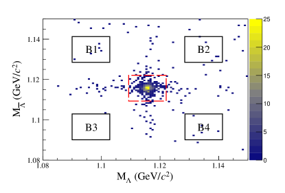
A secondary vertex fit is performed to obtain the decay vertex of the candidate, and the candidate is reconstructed by fitting the tracks to a common decay vertex. If there is more than one candidate, the one with the minimum chi-square value of the secondary vertex fit is selected. The reconstructed mass of candidate is required to be within 6.4 MeV of the nominal mass () Workman et al. (2022), as shown in Fig. 2. There is no requirement on the decay length of . Both a and a are required in mode I, while either a or a is required in mode II.
Information on the electromagnetic showers in the EMC is used to select the photon candidates. It is required that the shower time is within 700 ns of the event’s start time to suppress electronic noise and energy deposits unrelated to the events. A photon candidate is selected if its deposited energy is greater than 0.4 GeV. For each candidate signal event, at least one photon is required which is considered as the ISR photon.
A kinematic fit is applied to further suppress background. For mode I, a four-constraint (4C) kinematic fit requiring energy-momentum conservation under the hypothesis of a final state is applied to the signal candidates. If there is more than one photon candidate, the combination with the minimum is selected. To suppress the background with one more photon than the signal process, we require , where and are the chi-square values under the hypotheses of and final states. For mode II, a one-constraint (1C) kinematic fit with a missing under the hypothesis of a final state is applied to the signal candidates. Combining all pairs with the reconstructed , 1C kinematic fits are applied with the invariant mass of being constrained to the nominal mass Workman et al. (2022) and the mass of being unconstrained. The combination with the minimum is selected, where is the chi-square of the 1C kinematic fit. A requirement of () is optimized for the signal candidates for mode I (mode II).
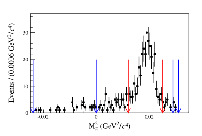
For the candidates of mode II, the distribution of the mass squared of the missing (), obtained from energy-momentum conservation, is shown in Fig. 3. To suppress background, a requirement of GeV is applied.
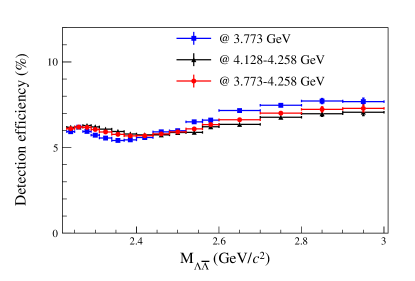
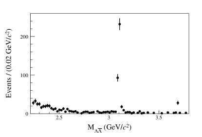
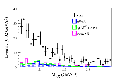
The distribution of the selection efficiencies obtained from signal MC samples as a function of invariant mass of () is shown in Fig. 4, where the efficiencies at the c.m. energies between 4.128 and 4.258 GeV are combined and weighted according to the effective luminosity of the ISR process. It should be noted that to improve the mass resolution of , we correct to . The mass resolution is given by the root-mean-square deviation of of the signal MC sample, where is the set value of the invariant mass of when generating the MC events. In this paper, the correction of the is implied unless specified. The spectrum of the accepted candidates from all data sets is shown in Fig. 5, in which 817 events are retained. The contributions from and decays are clearly seen. About 60% of the signal candidates have below 3.00 GeV/, and the number of signal candidates () in each interval is listed in the first column of Table 2.
IV BACKGROUND ANALYSIS
Potential background channels are investigated in the inclusive MC samples with a topology analysis Zhou et al. (2021); they consist of channels containing and channels without . The background channels containing , such as the processes of , , and with decaying to , are studied individually, while the non- background is estimated with the sideband method.
Events of are easily mistaken as signal events if a soft photon from the high-energy is missing. A data-driven method is used to estimate their contribution. A sample of events is selected from data, and its background is estimated with the sideband method. The sideband regions are chosen in the distribution of the invariant mass of (). The number of events of this sample is calculated by , where and are the numbers of events from the signal and the sideband regions of the sample, respectively. Next, the contribution from the remaining background () in the signal candidates is determined by:
| (4) |
where and are the numbers of the events selected by the signal and selection criteria from the MC sample. The MC sample is generated with the ConExc Ping (2014) event generator up to ISR LO, and the lineshape is obtained with the data sets collected at c.m. energies from 2.644 GeV to 3.080 GeV by BESIII.
In the reaction , the decays to with a branching ratio of 100% Workman et al. (2022), where the has low energy. Therefore, if the photon from the decay is missing, this event can be misidentified as signal. To estimate the background from this reaction, a MC sample with a total of 2 million events is generated with the ConExc Ping (2014) event generator up to ISR LO, and the lineshape used to generate the MC events is determined with the data sets collected at c.m. energies from 2.309 GeV to 3.080 GeV by BESIII. After applying the signal () selection criteria to this sample, we obtain the number of the surviving events (). A scaling factor is obtained by , where is the expected number of the events estimated with the cross section lineshape, and is the number of MC simulated events. Finally, the number of background events () is estimated by . Some other background channels, such as the processes and , are negligible.
Next, the sideband method is used to study the non- background. For mode I, two-dimensional (2D) sideband regions of versus are adopted, and for mode II, one-dimensional (1D) sideband regions in the distribution of are used. The distributions of and of inclusive MC samples after removing the channels containing the pair are nearly flat, so it is reasonable to use the sideband method. The 2D sideband regions (shown in Fig. 2) are chosen as: B1: GeV and GeV; B2: GeV and GeV; B3: GeV and GeV; and B4: GeV and GeV. The 1D sideband regions (shown in Fig. 3) are chosen as GeV and GeV. The numbers of events from sideband regions of data () are calculated by:
| (5) |
where and are the numbers of the events from the 2D and 1D sideband regions of data, respectively. The same sideband regions are used for the and MC samples, and the numbers of events from sideband regions of these MC samples () are obtained with Eq. (5). The number of non- background events () is estimated by:
| (6) |
The numbers of events for the three main background channels above (, , ) are calculated in each interval when measuring the Born cross section.
The distributions of of the main background events from all data sets are shown in Fig. 6, and the numbers of background events over all data sets for the three main background channels in each interval are listed in Table 2.
| (GeV) | ||||
| 2.231-2.250 | 28.0 5.3 | 1.9 1.2 | 1.28 0.05 | 0.63 0.70 |
| 2.25-2.27 | 32.0 5.7 | 0.7 | 1.35 0.05 | 0.41 |
| 2.27-2.29 | 25.0 5.0 | 1.4 0.6 | 1.36 0.05 | 2.67 1.22 |
| 2.29-2.31 | 24.0 4.9 | 1.3 0.6 | 1.37 0.05 | 0.69 0.71 |
| 2.31-2.34 | 28.0 5.3 | 2.4 0.7 | 2.00 0.07 | 0.08 |
| 2.34-2.37 | 27.0 5.2 | 4.2 0.9 | 1.83 0.05 | 0.11 |
| 2.37-2.40 | 34.0 5.8 | 5.2 0.9 | 1.54 0.05 | 0.32 |
| 2.40-2.44 | 28.0 5.3 | 3.5 0.8 | 1.74 0.05 | 0.10 |
| 2.44-2.48 | 23.0 4.8 | 3.3 0.7 | 1.53 0.05 | 0.32 |
| 2.48-2.52 | 16.0 4.0 | 3.3 0.7 | 1.28 0.05 | 1.22 |
| 2.52-2.56 | 19.0 4.4 | 1.7 0.5 | 1.01 0.05 | 1.51 0.90 |
| 2.56-2.60 | 18.0 4.2 | 1.4 0.5 | 0.87 0.05 | 0.21 |
| 2.60-2.70 | 24.0 4.9 | 1.4 0.5 | 1.74 0.05 | 0.39 |
| 2.70-2.80 | 15.0 3.9 | 1.5 0.5 | 1.12 0.04 | 3.00 1.25 |
| 2.80-2.90 | 15.0 3.9 | 2.3 0.6 | 0.73 0.03 | 0.07 |
| 2.90-3.00 | 18.0 4.2 | 2.6 0.7 | 0.49 0.03 | 0.36 |
V SYSTEMATIC UNCERTAINTY
Several sources of systematic uncertainties are considered in the cross section measurement. The combined results of different reconstructed methods and different data sets are summarized in Tables 3 and 4 for the correlated and uncorrelated parts, respectively. The correlated and uncorrelated parts are summed in quadrature to determine the total uncertainty.
| Source | Uncertainty |
| Luminosity | 1.1 |
| reconstruction | 2.1 |
| reconstruction | 2.8 |
| 1.6 | |
| tracking and PID | 0.7 |
| window | 0.6 |
| ISR photon detection | 1.0 |
| Kinematic fit | 1.7 |
| Neglected background | 1.5 |
| Total | 4.7 |
| (GeV) | non- | Ang | MC | Total | ||
| 2.231-2.250 | 0.3 | 0.6 | 0.4 | 2.7 | 1.6 | 3.2 |
| 2.25-2.27 | 0.1 | 0.9 | 1.4 | 0.6 | 1.4 | 2.2 |
| 2.27-2.29 | 0.7 | 1.8 | 0.5 | 2.3 | 4.1 | 5.1 |
| 2.29-2.31 | 0.9 | 1.9 | 0.4 | 2.2 | 0.7 | 3.1 |
| 2.31-2.34 | 1.3 | 3.6 | 0.5 | 2.7 | 1.5 | 4.9 |
| 2.34-2.37 | 0.8 | 3.0 | 0.4 | 1.6 | 0.9 | 3.6 |
| 2.37-2.40 | 1.0 | 2.0 | 3.3 | 0.3 | 0.9 | 4.1 |
| 2.40-2.44 | 0.6 | 3.0 | 0.4 | 0.8 | 0.8 | 3.2 |
| 2.44-2.48 | 0.5 | 2.4 | 0.5 | 1.7 | 2.2 | 3.6 |
| 2.48-2.52 | 1.6 | 5.2 | 5.2 | 2.2 | 2.2 | 8.2 |
| 2.52-2.56 | 1.0 | 5.4 | 0.9 | 1.7 | 3.3 | 6.7 |
| 2.56-2.60 | 0.5 | 2.9 | 0.4 | 0.8 | 1.8 | 3.6 |
| 2.60-2.70 | 0.9 | 3.2 | 0.9 | 2.5 | 1.4 | 4.4 |
| 2.70-2.80 | 7.1 | 9.3 | 24.8 | 2.1 | 1.9 | 27.5 |
| 2.80-2.90 | 1.7 | 2.3 | 2.3 | 2.1 | 1.5 | 4.4 |
| 2.90-3.00 | 1.2 | 1.5 | 0.3 | 1.9 | 5.4 | 6.0 |
The integrated luminosity is measured with an uncertainty of 0.5% at GeV and an uncertainty of 1.0% at other c.m. energies Ablikim et al. (2016b, 2015a, 2022c). In this analysis, the effective luminosity of the ISR process is calculated based on Eq. (3), and a 0.5% uncertainty is estimated Noh (2021). Thus, the total systematic uncertainty on the luminosity is 0.8% at GeV and 1.2% at other energy points.
The uncertainties from the reconstruction of and are studied by a control sample of , and determined to be 2.8% and 3.8% at GeV, and 2.6% and 3.4% at other energy points, respectively. A 1.0% uncertainty is taken for the ISR photon detection Ablikim et al. (2019c).
For mode II, the uncertainties due to the tracking and PID are 1.0% for each Ablikim et al. (2015b). The uncertainty due to the window is also studied by the control sample of , and estimated as 1.4% (0.8%) at GeV, and 1.5% (0.9%) at other energy points. The uncertainty due to the branching fraction of , , is obtained from the PDG Workman et al. (2022) to be 1.6%.
The uncertainty from the kinematic fit is divided into two parts: the contribution of the ISR photon and the contribution of the remainder. The former is determined by a control sample of the radiative Bhabha process , and estimated as 0.4%, 0.2% and 1.1% for the cases of full reconstruction, missing and missing , respectively. The later is studied by a control sample of , and is 0.2% (0.2%), 2.4% (2.2%) and 2.2% (2.2%) at GeV (other energy points), for the cases of full reconstruction, missing and missing , respectively. Thus, the uncertainty due to the kinematic fit at GeV (other energy points) is 0.6% (0.6%), 2.6% (2.4%) and 3.3% (3.3%) for the cases of full reconstruction, missing and missing , respectively.
The signal MC samples are generated with PHSP. The angular distribution of the pair, the spin correlation between and , and the polarization of decay are not taken into account. To estimate the uncertainty due to these factors, signal MC samples with an angular amplitude including these effects are generated. The parameterization of the angular amplitude is the same as that in Ref. Ablikim et al. (2019a), and the corresponding parameters are cited from it when GeV and obtained with the data set at GeV when GeV. The relative difference of the detection efficiency to that of the PHSP mode is regarded as the uncertainty.
The uncertainty from the MC model is considered by changing the event generator from ConExc Ping (2014) to PHOKHARA10.0 pho . The relative difference of the detection efficiency of these two event generators is taken as the uncertainty.
For the channel of , the sideband regions on the spectrum are used to estimate the background of the sample. Here, the 2D sideband regions (sideband of and ) and 3D sideband regions (sideband of , and ) are also used. The values of and are obtained, where is the number of signal events, , and are the estimated numbers of events based on , 2D and 3D sidebands, respectively. The larger of the two values is taken as the uncertainty of this channel.
For the channel of , one of the parameters of the lineshape is changed by adding and subtracting a standard deviation (). Based on the different lineshapes, different estimated numbers of events are obtained. Further, the same method as for the channel is used here to obtain the uncertainty of this channel.
For the non- background, we move the sideband regions by 0.002 GeV/ and 0.002 GeV towards the signal for the 2D and the 1D sidebands, respectively, and obtain the new estimated numbers of non- background events. The relative difference between the old and new results is regarded as the uncertainty. For the interval of 2.70-2.80 GeV, since is extremely small () at GeV, the estimation of this uncertainty at GeV is significantly larger than that in other intervals. Except for the three main background sources mentioned above, several other background channels are neglected, and their contribution is considered as a systematic uncertainty, which is 2.2% at GeV and 1.1% at other energy points.
In this analysis, twelve data sets are used and three reconstruction methods (full reconstruction, and partial reconstruction with missing or ) are applied. We divide the data sets into two groups, where the first group only includes the data set at 3.773 GeV and the second group includes the other data sets at c.m. energies from 4.128 to 4.258 GeV. The uncertainties of the second group are studied together or inherited from the result at GeV. Thus, the systematic uncertainties are combined in two steps, where the first step combines the three reconstruction methods in each group and the second step combines the two groups. Uncertainties of the three reconstruction methods (two data set groups) are combined as the average value weighted by detection efficiencies (products of detection efficiency and effective luminosity). The weighted average formula is:
| (7) |
with
| (8) |
where , and with () are the weight, systematic uncertainty and efficiency for the reconstruction method (data set group) , and is the correlation parameter for two different reconstruction methods (data set groups) and , and is the effective luminosity for the data set group . For the systematic uncertainties arising from background the values are set to 0, and for other systematic uncertainties the are set to 1.
VI Results of the Cross section
The cross section for is calculated from the spectrum by:
| (9) |
where is the spectrum of data corrected for resolution effects after subtracting the background, is the detection efficiency from MC simulation as a function of , and Workman et al. (2022). The effective ISR luminosity is calculated by , where is described by Eq. (3). This effective luminosity includes the first-order radiative correction but does not take into account VP, so the obtained cross section is the “dressed” cross section.
The dependence of the mass resolution on is determined, and accordingly the is divided into 16 intervals from the threshold up to 3.00 GeV. To reduce the impact of the mass resolution, the width of the bin is at least 5 times larger than the mass resolution, so we do not correct the mass spectrum for resolution effects. The measured cross sections for the process in these intervals are listed in Table 5. A comparison between the results of this work and those of previous ones Ablikim et al. (2018a, 2019a); Bisello et al. (1990); Aubert et al. (2007) is displayed in Fig. 7.
| (GeV/) | (pb-1) | (pb) | ||
| 2.231-2.250 | 24.1 5.5 | 0.061 | 3.95 | 245 56 14 |
| 2.25-2.27 | 30.3 | 0.062 | 4.24 | 283 15 |
| 2.27-2.29 | 19.5 5.2 | 0.062 | 4.32 | 179 48 13 |
| 2.29-2.31 | 20.7 5.0 | 0.061 | 4.41 | 190 46 11 |
| 2.31-2.34 | 23.5 | 0.059 | 6.78 | 144 9.8 |
| 2.34-2.37 | 20.8 | 0.058 | 6.99 | 126.6 7.5 |
| 2.37-2.40 | 27.6 | 0.057 | 7.20 | 165 11 |
| 2.40-2.44 | 22.7 | 0.057 | 9.95 | 98.1 5.6 |
| 2.44-2.48 | 18.5 | 0.058 | 10.37 | 75.2 4.5 |
| 2.48-2.52 | 10.2 | 0.059 | 10.82 | 38.9 3.7 |
| 2.52-2.56 | 14.7 4.5 | 0.061 | 11.30 | 52.4 16.0 4.3 |
| 2.56-2.60 | 15.9 | 0.063 | 11.80 | 52.1 3.1 |
| 2.60-2.70 | 21.2 | 0.066 | 31.96 | 24.6 1.6 |
| 2.70-2.80 | 9.4 4.1 | 0.070 | 35.96 | 9.1 4.0 2.6 |
| 2.80-2.90 | 11.9 | 0.072 | 40.76 | 9.9 0.7 |
| 2.90-3.00 | 14.5 | 0.073 | 46.59 | 10.5 0.8 |
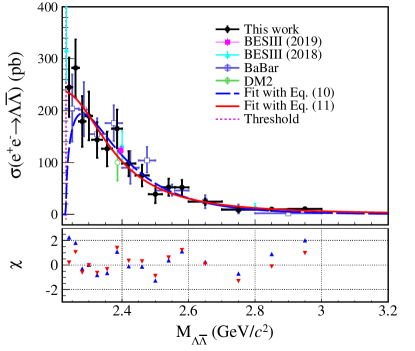
A search for a threshold effect is made by performing a least chi-square fit to the cross section from the production threshold up to 3.00 GeV with different assumed functions. The systematic uncertainty is included in the fit with the correlated and uncorrelated parts considered separately.
The first fit function is a perturbative QCD (pQCD) driven energy power function Pacetti et al. (2015)
| (10) |
where and are free parameters and the Coulomb correction factor is for neutral baryons. The fit result is shown as the blue dashed line in Fig. 7, with pbGeV10, GeV and the fit quality .
In Fig. 7, the pQCD prediction does not describe the anomalous enhancement well near threshold. Therefore, inspired by the results of cross section measurements of and Ablikim et al. (2021a, 2020a), it is assumed that there is a step near the threshold for the cross section, the threshold enhancement effect. By taking into account the strong interaction near the threshold instead of using the formula of Eq. (10), which contains the Coulomb factor, the cross section can be expressed as Ablikim et al. (2020a):
| (11) |
where , , and are three free parameters. The symbol represents the strong running coupling constant and is parameterized as:
| (12) |
where 91.1876 GeV Workman et al. (2022) is the mass of boson and 0.11856. This fit has , with , GeV and , and the fit result is shown as the red solid line in Fig. 7.
VII Study of the decay
The branching fraction of , , is determined via the ISR process at and GeV. After integrating over the photon polar angle, the cross section for ISR production of a narrow resonance (vector meson ), such as , decaying into the final state is given by Benayoun et al. (1999):
| (13) |
where and are the mass and electronic width of the vector meson , , is the branching fraction of , and is calculated by Eq. (3). If the cross section is measured, the branching fraction can be calculated by Eq. (13). The cross section can also be written as:
| (14) |
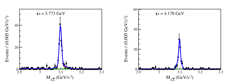
where is the number of events, is the detection efficiency, and is the integrated luminosity of data, whose values are listed in Table 1. The detection efficiency is estimated from MC simulation as 7.2% at GeV and 7.1% at GeV. The angular distribution of in decay is described by with Ablikim et al. (2017). To determine , using as a shared parameter, a simultaneous fit is performed with a double Gaussian function for the resonance and a linear function for the background and the continuum contribution, and the result is shown in Fig. 8
For the systematic uncertainties on the measurement of , the uncertainties of the luminosity, and reconstruction, tracking and PID, window, ISR photon detection, , and kinematic fit are the same as the cross section measurement. The uncertainty due to the MC model is assigned as 1.3%, by changing the model for the generation of the decay. The uncertainty of the fit region is determined by changing the fit region from (2.90, 3.30) GeV to a wider (2.80, 3.30) GeV and a narrower interval (3.00, 3.20) GeV to be 1.3%. The uncertainty from the signal model of the fit is estimated by changing the model from the double Gaussian function to the MC-shape-convolved Gaussian function as 1.3%. The uncertainty of the background model of the fit is estimated by changing the model from a linear function to a constant as 0.5%. Finally, we consider a systematic uncertainty due to the non- background. The non- background is treated as a peaking background, instead of a non-peaking one as default. The relative difference between the results of the two strategies, 1.9%, is regarded as the uncertainty. The total uncertainty is obtained to be 5.6% by summing all uncertainties in quadrature.
is determined to be , where the first uncertainty is statistical and the second is systematic. It is consistent with the PDG value Workman et al. (2022) within 2.
VIII Summary and discussion
Based on data sets corresponding to a total integrated luminosity of 11.957 fb-1 collected at twelve c.m. energies between 3.773 and 4.258 GeV with the BESIII detector at BEPCII, the cross section for the process is measured as the function of in 16 intervals from the production threshold up to 3.00 GeV using ISR events with the ISR photon tagged. A partial reconstruction method allowing a charged to be missing is used in addition to the full reconstruction method to increase the efficiency. In the first interval ranging from the threshold up to 2.25 GeV (with the width of 19 MeV), the cross section is determined to be pb, where the first uncertainty is statistical and the second is systematic. It is a non-zero value with a statistical significance of 4.3 and larger than the pQCD prediction by 2.3. In the region from 2.23 GeV up to 3.00 GeV, the cross section is measured in 15 intervals. The results are consistent with previous measurements at BaBar and BESIII. The spectrum of the cross section is fitted with the pQCD assumption and with the assumption of a step existing near threshold, with the latter being a better description of the data.
Acknowledgements.
The BESIII Collaboration thanks the staff of BEPCII, the IHEP computing center and the supercomputing center of USTC for their strong support. This work is supported in part by National Key R&D Program of China under Contracts Nos. 2020YFA0406400, 2020YFA0406300; National Natural Science Foundation of China (NSFC) under Contracts Nos. 11635010, 11735014, 11835012, 11935015, 11935016, 11935018, 11961141012, 12022510, 12025502, 12035009, 12035013, 12192260, 12192261, 12192262, 12192263, 12192264, 12192265, 12275320, 11625523, 11705192, 11950410506, 12061131003, 12105276, 12122509; the Chinese Academy of Sciences (CAS) Large-Scale Scientific Facility Program; the CAS Center for Excellence in Particle Physics (CCEPP); Joint Large-Scale Scientific Facility Funds of the NSFC and CAS under Contracts Nos. U1832207, U1732263, U1832103, U2032111; CAS Key Research Program of Frontier Sciences under Contracts Nos. QYZDJ-SSW-SLH003, QYZDJ-SSW-SLH040; 100 Talents Program of CAS; The Institute of Nuclear and Particle Physics (INPAC) and Shanghai Key Laboratory for Particle Physics and Cosmology; ERC under Contract No. 758462; European Union’s Horizon 2020 research and innovation programme under Marie Sklodowska-Curie grant agreement under Contract No. 894790; German Research Foundation DFG under Contracts Nos. 443159800, 455635585, Collaborative Research Center CRC 1044, FOR5327, GRK 2149; Istituto Nazionale di Fisica Nucleare, Italy; Ministry of Development of Turkey under Contract No. DPT2006K-120470; National Research Foundation of Korea under Contract No. NRF-2022R1A2C1092335; National Science and Technology fund; National Science Research and Innovation Fund (NSRF) via the Program Management Unit for Human Resources & Institutional Development, Research and Innovation under Contract No. B16F640076; Polish National Science Centre under Contract No. 2019/35/O/ST2/02907; The Royal Society, UK under Contracts Nos. DH140054, DH160214; The Swedish Research Council; U. S. Department of Energy under Contract No. DE-FG02-05ER41374.References
- Cabibbo and Gatto (1961) N. Cabibbo and R. Gatto, Phys. Rev. 124, 1577 (1961).
- Brodsky and Lebed (2009) S. J. Brodsky and R. F. Lebed, Phys. Rev. Lett. 102, 213401 (2009).
- Ablikim et al. (2020a) M. Ablikim et al. (BESIII), Phys. Rev. Lett. 124, 042001 (2020a).
- Lees et al. (2013) J. P. Lees et al. (BaBar), Phys. Rev. D 87, 092005 (2013).
- Ablikim et al. (2021a) M. Ablikim et al. (BESIII), Nature Phys. 17, 1200 (2021a).
- Aubert et al. (2007) B. Aubert et al. (BaBar), Phys. Rev. D 76, 092006 (2007).
- Ablikim et al. (2018a) M. Ablikim et al. (BESIII), Phys. Rev. D 97, 032013 (2018a).
- Ablikim et al. (2019a) M. Ablikim et al. (BESIII), Phys. Rev. Lett. 123, 122003 (2019a).
- Bisello et al. (1990) D. Bisello et al. (DM2), Z. Phys. C 48, 23 (1990).
- Ablikim et al. (2021b) M. Ablikim et al. (BESIII), Phys. Lett. B 814, 136110 (2021b).
- Ablikim et al. (2022a) M. Ablikim et al. (BESIII), Phys. Lett. B 831, 137187 (2022a).
- Ablikim et al. (2021c) M. Ablikim et al. (BESIII), Phys. Rev. D 103, 012005 (2021c).
- Ablikim et al. (2021d) M. Ablikim et al. (BESIII), Phys. Lett. B 820, 136557 (2021d).
- Ablikim et al. (2018b) M. Ablikim et al. (BESIII), Phys. Rev. Lett. 120, 132001 (2018b).
- Huang and Ferroli (2021) G. Huang and R. B. Ferroli (BESIII), Natl. Sci. Rev. 8, nwab187 (2021).
- Lees et al. (2012) J. P. Lees et al. (BaBar), Phys. Rev. D 86, 012008 (2012).
- Ablikim et al. (2019b) M. Ablikim et al. (BESIII), Phys. Rev. D 100, 032009 (2019b).
- Haidenbauer and Meißner (2016) J. Haidenbauer and U. G. Meißner, Phys. Lett. B 761, 456 (2016).
- Cao et al. (2018) X. Cao, J. P. Dai, and Y. P. Xie, Phys. Rev. D 98, 094006 (2018).
- Yang et al. (2019) Y. Yang, D. Y. Chen, and Z. Lu, Phys. Rev. D 100, 073007 (2019).
- Baldini et al. (2009) R. Baldini, S. Pacetti, A. Zallo, and A. Zichichi, Eur. Phys. J. A 39, 315 (2009).
- Druzhinin et al. (2011) V. P. Druzhinin, S. I. Eidelman, S. I. Serednyakov, and E. P. Solodov, Rev. Mod. Phys. 83, 1545 (2011).
- Kuraev and Fadin (1985) E. A. Kuraev and V. S. Fadin, Sov. J. Nucl. Phys. 41, 466 (1985).
- Ablikim et al. (2010) M. Ablikim et al. (BESIII), Nucl. Instrum. Meth. A 614, 345 (2010).
- Wang (2006) Y. F. Wang, Int. J. Mod. Phys. A 21, 5371 (2006).
- Ablikim et al. (2020b) M. Ablikim et al. (BESIII), Chin. Phys. C 44, 040001 (2020b).
- Huang et al. (2022) K. X. Huang et al., Nucl. Sci. Tech. 33, 142 (2022).
- (28) X. Li et al., Radiat. Detect. Technol. Methods 1, 13 (2017).
- (29) Y. X. Guo et al., Radiat. Detect. Technol. Methods 1, 15 (2017).
- Cao et al. (2020) P. Cao et al., Nucl. Instrum. Meth. A 953, 163053 (2020).
- Agostinelli et al. (2003) S. Agostinelli et al. (GEANT4), Nucl. Instrum. Meth. A 506, 250 (2003).
- Ping (2014) R. G. Ping, Chin. Phys. C 38, 083001 (2014).
- (33) Monte Carlo event generator PHOKHARA webpage: http://ific.uv.es/ rodrigo/phokhara/.
- Li et al. (2022) Z. Y. Li, A. X. Dai, and J. J. Xie, Chin. Phys. Lett. 39, 011201 (2022).
- Ablikim et al. (2022b) M. Ablikim et al. (BESIII), Phys. Rev. Lett. 128, 062004 (2022b).
- Jadach et al. (2001) S. Jadach, B. F. L. Ward, and Z. Was, Phys. Rev. D 63, 113009 (2001).
- Jadach et al. (2000) S. Jadach, B. F. L. Ward, and Z. Was, Comput. Phys. Commun. 130, 260 (2000).
- Ping (2008) R. G. Ping, Chin. Phys. C 32, 599 (2008).
- Bonneau and Martin (1971) G. Bonneau and F. Martin, Nucl. Phys. B 27, 381 (1971).
- Lange (2001) D. J. Lange, Nucl. Instrum. Meth. A 462, 152 (2001).
- Ablikim et al. (2016a) M. Ablikim et al. (BESIII), Chin. Phys. C 40, 063001 (2016a).
- Ablikim et al. (2021e) M. Ablikim et al. (BESIII), Chin. Phys. C 45, 103001 (2021e).
- Ablikim et al. (2016b) M. Ablikim et al. (BESIII), Phys. Lett. B 753, 629 (2016b), [Erratum: Phys. Lett. B 812, 135982 (2021)].
- Ablikim et al. (2015a) M. Ablikim et al. (BESIII), Chin. Phys. C 39, 093001 (2015a).
- Ablikim et al. (2022c) M. Ablikim et al. (BESIII), Chin. Phys. C 46, 113002 (2022c).
- Workman et al. (2022) R. L. Workman et al. (Particle Data Group), PTEP 2022, 083C01 (2022).
- Zhou et al. (2021) X. Zhou, S. Du, G. Li, and C. Shen, Comput. Phys. Commun. 258, 107540 (2021).
- Noh (2021) C. Noh, New Phys. Sae Mulli 71, 1096 (2021).
- Ablikim et al. (2019c) M. Ablikim et al. (BESIII), Phys. Rev. D 99, 011101 (2019c).
- Ablikim et al. (2015b) M. Ablikim et al. (BESIII), Phys. Rev. D 91, 112004 (2015b).
- Pacetti et al. (2015) S. Pacetti, R. Baldini Ferroli, and E. Tomasi-Gustafsson, Phys. Rept. 550-551, 1 (2015).
- Benayoun et al. (1999) M. Benayoun, S. I. Eidelman, V. N. Ivanchenko, and Z. K. Silagadze, Mod. Phys. Lett. A 14, 2605 (1999).
- Ablikim et al. (2017) M. Ablikim et al. (BESIII), Phys. Rev. D 95, 052003 (2017).